py-MCMD: Python Software for Performing Hybrid Monte Carlo/Molecular Dynamics Simulations with GOMC and NAMD

Abstract

py-MCMD, an open-source Python software, provides a robust workflow layer that manages communication of relevant system information between the simulation engines NAMD and GOMC and generates coherent thermodynamic properties and trajectories for analysis. To validate the workflow and highlight its capabilities, hybrid Monte Carlo/molecular dynamics (MC/MD) simulations are performed for SPC/E water in the isobaric–isothermal (NPT) and grand canonical (GC) ensembles as well as with Gibbs ensemble Monte Carlo (GEMC). The hybrid MC/MD approach shows close agreement with reference MC simulations and has a computational efficiency that is 2 to 136 times greater than traditional Monte Carlo simulations. MC/MD simulations performed for water in a graphene slit pore illustrate significant gains in sampling efficiency when the coupled–decoupled configurational-bias MC (CD–CBMC) algorithm is used compared with simulations using a single unbiased random trial position. Simulations using CD–CBMC reach equilibrium with 25 times fewer cycles than simulations using a single unbiased random trial position, with a small increase in computational cost. In a more challenging application, hybrid grand canonical Monte Carlo/molecular dynamics (GCMC/MD) simulations are used to hydrate a buried binding pocket in bovine pancreatic trypsin inhibitor. Water occupancies produced by GCMC/MD simulations are in close agreement with crystallographically identified positions, and GCMC/MD simulations have a computational efficiency that is 5 times better than MD simulations. py-MCMD is available on GitHub at https://github.com/GOMC-WSU/py-MCMD.

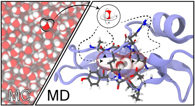
Graphical Abstract

INTRODUCTION

Molecular dynamics (MD) simulations are an essential tool for understanding biological structure and function. Simulations of systems containing 100 000 atoms are routine, and simulations of up to 2 billion atoms have been made possible through advances in hardware and MD codes.¹ For moderate-sized systems, microsecond and even millisecond time scales are attainable nowadays.^2,3 MD simulations are used routinely for computational drug discovery,^4–6 determination of lipid bilayer mechanical and transport properties,^2,7–10 and elucidation of protein function.^11–13 Since all atomic positions are known at any moment in time, MD simulations provide spatial and temporal resolutions that are not currently achievable with experiments, and therefore, the method can be viewed as a “computational microscope”^14,15 in the quest to understand biological machinery.

While the MD methodology is broadly applicable to the study of biological molecules, there are certain problems that may be better suited to alternative sampling approaches. Notable examples include diffusion through pores and membranes,¹⁶ the hydration state of buried pockets or channels in proteins,^17–21 the formation of nanodomains,³ and phase separation in multicomponent lipid bilayers.^22,23 These systems contain high free energy barriers, which may prevent reliable sampling of phase space during conventional MD simulation time scales, or require the use of an open system, i.e., allowing for changes in the number of molecules.

An alternative strategy to running longer simulations is to incorporate Monte Carlo (MC) moves into MD simulations.^{17,19–21,23–26} In this hybrid approach, trial MC moves are proposed, which are accepted or rejected on the basis of statistical mechanical probabilities. These MC moves may use alternative, or “unphysical”, pathways that allow the system to traverse high free energy barriers. The inclusion of MC moves also provides the opportunity to simulate systems in the grand canonical (GC) ensemble, where the number of constituent molecules can change during the simulation.

The use of grand canonical Monte Carlo (GCMC) sampling in MD simulations has been shown to produce significant improvements in the accuracy and precision of ligand–protein binding free energies.^{20,21,24,27,28} GCMC sampling for water in the binding pocket leads to rapid equilibration, compared with the slower diffusion observed in MD, particularly for buried sites. GCMC, using dual control volumes,¹⁶ has been combined with Brownian dynamics (GCMC–BD) to simulate the movement of ions through transmembrane pores.^29,30 The inclusion of an MC identity-exchange move, using either configurational-bias sampling²² or a combination of alchemical transformation and nonequilibrium MD,²³ to sample phase space has been used to greatly accelerate the equilibration of multicomponent lipid bilayers.

Basic GC functionality is present in a number of MD codes^{17,19,25,26,31} in a variety of forms: either integrated into the code, as has been done in CHARMM,^17,31 AMBER,¹⁹ and LAMMPS,³² or interfaced through external Python codes for GROMACS²⁵ and OPENMM.²⁶ Additional MC moves are available in OpenMM³³ through the OpenMMTools package.³⁴ Some implementations use the cavity-bias method to improve acceptance rates for the transfer of water molecules,³⁵ while in others only random insertions are possible.

This work describes hybrid MC/MD simulations that utilize NAMD for MD and GOMC for MC. These codes are linked with py-MCMD, an open-source Python program that oversees information transfer and the execution of each code.³⁶ By linking of GOMC with NAMD, it is possible to perform hybrid GCMC/MD simulations that utilize the full suite of advanced configurational-bias sampling algorithms that are available in GOMC.^37–40 With py-MCMD, it is also possible to integrate MD sampling of configurational space into MC simulations, such as Gibbs ensemble (GE),⁴¹ leading to enhanced sampling efficiency over standard Gibbs ensemble Monte Carlo (GEMC) simulations.⁴²

To validate the py-MCMD program and assess its computational efficiency, a series of MC/MD simulations were performed for water in the isothermal–isobaric (NPT) and GC ensembles as well as with the GE method. Additional hybrid MC/MD simulations were performed in the canonical (NVT) ensemble with an intrabox swap move for water in a graphene slit pore and in the GC ensemble to determine the hydration state of a buried binding site in bovine pancreatic trypsin inhibitor (BPTI). Notably, NVT MC/MD simulations of water in a graphene slit pore, performed with coupled–decoupled configurational-bias MC (CD–CBMC), equilibrated in 25 times fewer cycles than simulations without CD–CBMC and 66 times fewer cycles than hybrid MC/MD simulations using the cavity-bias method.¹⁹ GCMC/MD simulations of the BPTI system showed rapid hydration of the buried binding pocket with a 5-fold improvement in computational efficiency compared with standard MD simulations.

METHODS

Workflow.

py-MCMD defines a hybrid MC/MD workflow that facilitates information transfer between GOMC and NAMD (Figure 1).³⁶ An additional Python analysis script was also created that combines the simulation trajectories and thermodynamic properties reported by NAMD and GOMC into several compact files for postsimulation analysis and visualization. GOMC version 2.70⁴⁰ was modified to read and write binary coordinate, velocity, and extended system control files in NAMD native format, which improves the accuracy of the hybrid simulations and reduces simulation startup time and disk space requirements. These modifications are available in the recently released GOMC version 2.75. py-MCMD was designed to work with NAMD version 2.14. The py-MCMD software and its documentation are available on GitHub at https://github.com/GOMC-WSU/py-MCMD.

Figure 1.

Schematic of the hybrid MC/MD workflow. In the initial cycle, MD simulations with or without restraints are used to minimize the energy of the system and perform a short dynamics simulation to eliminate unfavorable configurations. This is followed by alternating cycles of MC and MD simulations. During the MC simulations, a variety of MC moves are utilized in each ensemble to satisfy equilibrium conditions, e.g., swap (transfer of a molecule between phases), intraswap (deletion and reinsertion of a molecule in a random new location in the same phase), or volume change (perturbing the volume of the system). MD simulations in the NVT ensemble are used for efficient sampling of configurations and conformations. Control of the simulation parameters, ensemble, and MC moves are possible through NAMD and GOMC control files (hexagons). Transfer of information between the MC and MD engines is overseen by the py-MCMD Python software.

The hybrid MC/MD workflow starts with a short conjugate-gradient energy minimization and NVT MD simulation to stabilize the system, which is followed by cycles of alternating MC and MD steps. Following the strategy of Gartner et al., the results of the MD simulation are always accepted,⁴² while all MC moves follow strict detailed balance. The choice to use nonmetropolized hybrid Monte Carlo was based on the following criteria: it produces correct results for reasonable choices of simulation parameters; it is computationally more efficient than metropolized hybrid Monte Carlo;⁴³ and the algorithm is straightforward to implement. It should be noted, however, that using the Brooks–Bruünger–Karplus (BBK) integrator⁴⁴ in Langevin dynamics simulations with a large time step will introduce a time-step-dependent bias⁴⁵ due to finite integration time step error.^43,46 Despite this bias, the BBK integrator does produce a configuration-space average that is close to the true ensemble average. In order to more accurately sample the exact configuration space, the BBK integrator should be used with an integration time step of ≤1 fs, or alternatively, the BAOAB integrator⁴⁷ can be used for better conservation of the configuration-space average with a 2 fs time step.^45,46

py-MCMD generates control files for GOMC and NAMD, sets run-time parameters, launches the appropriate simulation engine at each point in the sequence, and checks the total system energies for consistency when switching between engines. Relative energy differences between NAMD and GOMC greater than 1 × 10⁻³ produce a warning message. Typical relative energy differences observed between GOMC and NAMD were on the order of 1 × 10⁻⁶ to 1 × 10⁻⁵. To maintain continuity of system dynamics, velocity information is passed through GOMC, even though it is not required for MC simulations. Any atoms that are moved or inserted during the Monte Carlo phase have their velocities initialized using a Maxwell–Boltzmann distribution.^48,49

All of the simulations were performed using a switched potential for Lennard–Jones (LJ) interactions using a 12 Å cutoff and a 10 Å switch distance. No long-range corrections were used for LJ interactions. Electrostatic interactions were calculated using the Ewald summation^50,51 in GOMC and particle-mesh Ewald^52,53 in NAMD. A tolerance of 10⁻⁵ and a real-space cutoff of 12 Å were used for electrostatic interactions. Molecule-transfer and intrabox swap moves were performed with the CD–CBMC method³⁷ using 16 trial positions for the first atom and eight trial positions for all remaining atoms.⁵⁴ A derivation of the CD–CBMC algorithm for flexible and rigid-body molecules is provided in the Supporting Information. A hard inner cutoff was used to reject any MC moves that placed atom centers closer than 1 Å.⁵⁵ In both MC and MD simulations, water was treated as a rigid-body molecule, with covalent bonds to hydrogen atoms constrained using the SETTLE algorithm⁵⁶ in the MD simulations. All of the simulations were performed using periodic boundary conditions with the minimum image convention. MD simulations were performed in the NVT ensemble using Langevin dynamics⁵⁷ with the BBK integrator scheme⁴⁴ to simulate the heat bath. For the MD simulations, the multiple-time-step r-RESPA algorithm⁵⁸ was used with a 2 fs integration time step, where short- and long-range forces were evaluated every 2 and 4 fs, respectively.

Workflow Validation: SPC/E Water.

To validate the workflow, hybrid MC/MD simulations were performed for SPC/E water⁵⁹ in the NPT, GC, and Gibbs ensembles, and the results were compared to reference MC simulations. A variety of Monte Carlo moves were used, which include rigid-body translation (translate), rigid-body rotation (rotate), volume exchange (volume), molecule transfer between phases (swap), and configurational-bias regrowth (regrowth). A summary of the MC move fractions and lengths of the MC and MD components for each system is provided in Table 1. A description of the MC moves used in this work, such as rigid-body displacement and rotation, configurational bias, and volume exchange are provided in the Supporting Information. Parameters for the SPC/E water model are listed in Table S1. For all of the hybrid MC/MD simulations, the numbers of MC trials and MD time steps were set to ensure that each cycle would result in at least one accepted MC move and one uncorrelated sample during the MD simulation. To calculate statistical uncertainties, each simulation was repeated five times, initiated with different random seeds and with unique initial configurations (coordinates and velocities) generated using the Molecular Simulation Design Framework (MoSDeF).^60–63

Table 1.

Summary of Simulation Parameters

simulation type			distribution of MC moves						simulation parameters
system	type	ensemble [T (K)]	volume	swap	intraswap	translate	rotate	regrowth	run lengtha	cycle (MCS: ps)	no. of replicas	output freq.
SPC/E water	MC	NPT [298]	0.01		0.24	0.25	0.25	0.25	3 × 107 MCS	N/A	5	1000 MCS
	MC/MD	NPT [298]	1.00						3 × 104 C	(20: 1.96)	5	20 MCS + 1.96 ps
	MC	GCMC [510]		0.50		0.15	0.15	0.20	1.5 × 108 MCS	N/A	5	1500 MCS
	MC/MD	GCMC [510]		1.00					1 × 105 C	(500: 2.0)	5	500 MCS + 2 ps
	MC	GEMC [500]	0.01	0.20	0.20	0.19	0.20	0.20	5 × 107 MCS	N/A	5	1500 MCS
	MC/MD	GEMC [500]	0.01	0.99					1.3 × 104 C	(500: 2.0)	5	500 MCS + 2 ps
	MC	GEMC [400]	0.01	0.20	0.20	0.19	0.20	0.20	5 × 107 MCS	N/A	5	1500 MCS
	MC/MD	GEMC [400]	0.01	0.99					1.3 × 104 C	(200: 2.6)	5	200 MCS + 2.6 ps
	MC	GEMC [300]	0.01	0.20	0.20	0.19	0.20	0.20	5 × 107 MCS	N/A	5	10000 MCS
	MC/MD	GEMC [300]	0.01	0.99					1.3 × 104 C	(7000: 6.0)	5	7000 MCS + 6 ps
slit pore (CD–CBMC)	MC/MD	NVT [500]			1.00				2 × 104 C	(1000: 2.0)	5	1000 MCS + 2 ps
slit pore (unbiased)	MC/MD	NVT [500]			1.00				2 × 104 C	(1000: 2.0)	5	1000 MCS + 2 ps
BPTI	MD	NVT [298]							10 ns	N/A	10	10 ps
	MC/MD	GCMC [298]		1.00b					1 × 103 C	(2000: 10.0)	10	2000 MCS + 10 ps

^aMCS, MC steps; C, cycles.

^bTargeted swap move.

Simulations in the NPT ensemble were performed at 298 K and 1.01325 bar for a system containing 1361 SPC/E water molecules with an initial density of 0.9496 g/cm³. GC ensemble simulations were performed at 510 K and a chemical potential of −4.9037 kcal/mol, with a box size of $\overline{V}=42875$ ų. GE simulations⁴¹ were performed at 300, 400, and 500 K to calculate the saturated liquid and vapor coexistence densities of SPC/E water. For the GE simulations at 500 K, the initial configurations for the vapor and liquid phases each included 500 molecules at a density of 0.295 g/cm³. The initial density of each phase was intentionally set far from equilibrium to verify the convergence of the MC/MD simulation. Initial densities for simulations at 300 and 400 K were set to the expected saturated liquid and vapor densities, generated from prior simulations of SPC/E water.⁶⁴

Computational Efficiency.

To calculate the computational efficiency of the hybrid MC/MD with respect to standard MC simulations, the integrated autocorrelation time (τ), statistical inefficiency (g = 1 + 2τ), and normalized fluctuation autocorrelation function (C(t)) observed during each simulation were calculated using the pymbar autocorrelation time analysis tool.^65,66 To accurately compare the computational efficiencies of the hybrid MC/MD and MC simulations, τ, g, and C(t) are reported in terms of computational cost (CPU hours) instead of number of simulation steps. g = 1 indicates that 1 CPU hour was required to generate an uncorrelated data point. All of the bulk water simulations were performed on four cores of an Intel Gold 5118 2.3 GHz CPU. Data points were written to disk with the frequencies listed in Table 1.

Data series were generated for autocorrelation analysis after equilibration was reached according to the reduced potential function f(R) appropriate to each ensemble.⁶⁵ The f(R) function for a particular microstate is given by

$$f(\mathbf{R})=-\beta [U(\mathbf{R})+PV(\mathbf{R})-\mu N(\mathbf{R})]$$ (1)

where R, U(R), V(R), and N(R) are the configuration, total potential energy, volume, and number of molecules in the system for a specific microstate, respectively, β = 1/k_BT, P is the imposed pressure, and μ is the imposed chemical potential. Depending on the ensemble, eq 1 combines temperature, potential energy, pressure, volume, number of molecules, and/or chemical potential to produce a reduced-value data series. The reduced potential functions used in this work for the NPT and μVT ensembles were −β[U(R) + PV(R)] and −β[U(R) − μN(R)], respectively. For GEMC simulations, the reduced potential used was f(R) = −β[U_liq(R) + U_gas(R)].

Illustrative Applications: Graphene Slit Pore and BPTI.

To illustrate the application of the py-MCMD software, two additional hybrid MC/MD simulations were performed in the NVT and GC ensembles, where achieving equilibrium using standard MD simulations is grossly inefficient or in some cases impossible (e.g., graphene slit pore equilibration). The NVT MC/MD simulations at 500 K were performed on SPC/E water in a rectangular box with dimensions of 29.5 Å × 29.8 Å × 85 Å that was partitioned into two regions by two impermeable graphene sheets placed at 28 Å apart from each other.¹⁹ Each graphene sheet contained 336 carbon atoms. Force field parameters for carbon atoms are listed in Table S1.⁶⁷ The outer region was filled initially with 1866 water molecules at a density of 1.197 g/cm³, while the inner region was populated with a single water molecule. To compare the efficiency of the CD–CBMC algorithm with simple MC sampling, additional simulations were performed using only one unbiased trial position for the intrabox swap move. Five independent NVT MC/MD simulations were performed to calculate statistical uncertainties, where each simulation was initiated with different random seeds, unique initial configurations, and velocities.

In the final example, GCMC/MD simulations were used to calculate the most probable water positions in the buried binding pocket of BPTI. The initial configuration was generated from the starting structure (PDB ID 5PTI),^68–71 without any hydrogen/deuterium atoms. The system was protonated and solvated in water with 15 Å of padding around the protein in each dimension, and neutralizing ions (0.15 mol/L NaCl) were added to the system using the QwikMD⁷² plugin in VMD.⁷³ The mTIP3P⁷⁴ and CHARMM36^75–83 force fields were used to represent water and protein interactions, respectively. The initial configuration was minimized for 2 ps and then annealed with NPT MD simulations from 60 to 298 K for 28.68 ps, followed by a 5 ns NPT MD equilibration at 298 K and 1.01325 bar. The Langevin piston method⁸⁴ was used for the barostat, which combines the Hoover constant-pressure equations of motion^85,86 with piston fluctuations controlled by Langevin dynamics.⁸⁴ During the equilibration, the protein’s backbone atoms were restrained using a harmonic potential with a 2 kcal mol⁻¹ Å⁻² force constant.

GCMC/MD simulations were performed at 298 K and a chemical potential of −6.3349 kcal/mol. This corresponds to the average equilibrium density of 1.0113 ± 0.0004 g/cm³ for bulk mTIP3P water, which is consistent with the density produced by NPT MD simulations at 298 K and 1.01325 bar.⁸⁷ Water molecules were inserted and deleted from a cube with a side length of 15 Å centered at the geometric center of the C_α atoms of the Tyr10 and Asn43 residues.²⁶ For these calculations, a hard inner cutoff for MC insertion/deletion moves was not used since all of the atoms in the mTIP3P water force field have Lennard–Jones parameters, minimizing the possibility of naked charges being placed in close proximity during an insertion attempt. Ten independent GCMC/MD simulations were performed for 1000 cycles, where each cycle consisted of 2000 MC steps and a 10 ps MD simulation. Each simulation was started with an empty binding pocket and a unique initial configuration, distribution of velocities, and random number seed. To prevent collapse of the binding pocket due to the absence of water, additional harmonic restraints with a 2 kcal mol⁻¹ Å⁻² force constant were applied to heavy atoms of the protein during the first cycle of the GCMC/MD simulations. The rest of the cycles were run without restraints.

To determine the most probable positions for each of the three water molecules within the binding pocket, the simulation trajectories were aligned, and water molecule positions observed during the simulation were clustered across trajectory frames using the average-linkage hierarchical clustering algorithm, as implemented by Samways et al.²⁶ A water molecule was considered to be clustered if its oxygen atom was within 2.4 Å of another water oxygen atom. To avoid clustering of waters within the same frame, the oxygen–oxygen distance of waters that belonged to the same frame in a trajectory was set to a large number (~10⁸ Å). Each cluster consisted of an array of oxygen positions, and the cluster centroid was calculated as the average of these oxygen positions. The most probable water positions were calculated on the basis of the oxygen position of the water molecule that is observed closest to the cluster centroid. The occupancy of clustered water was calculated as the ratio of total observed waters in the cluster to the number of frames in the trajectory. Clustered water positions were assigned to a specific crystallographic water site (e.g., site 1, 2, or 3) if they were within 1.5 Å of one crystallographic water site and not closer to any others.

RESULTS AND DISCUSSION

Workflow Validation: SPC/E Water.

To validate the hybrid MC/MD workflow, SPC/E water simulations were performed in the isobaric–isothermal (NPT), and grand canonical (GC) ensembles. Calculations were also performed with the Gibbs ensemble (GE) Monte Carlo method. As shown in Figure 2, close agreement was achieved between the trajectories generated with MC/MD and standard MC simulations.

Figure 2.

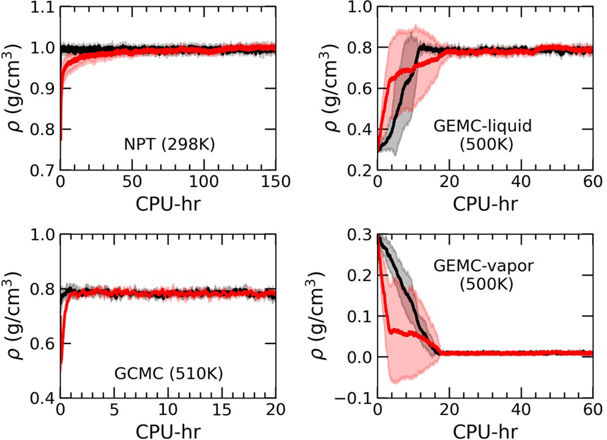
Predictions of MC/MD (black) and MC (red) simulations as functions of computational cost (CPU-hr) in various ensembles for SPC/E water: NPT at 298 K and 1.01325 bar; GCMC at 510 K and a chemical potential of −4.9037 kcal/mol; GEMC at 500 K liquid and vapor densities. Solid lines correspond to averages over five replicas, while the shaded areas represent the standard deviations calculated from the five independent replicas.

NPT simulations at 298 K and 1.01325 bar were purposefully started from an artificially low density of 0.9496 g/cm³ to test the convergence behavior of the MC/MD simulations. Figure 2 shows that the MC/MD simulations converged to the correct density (0.9939 ± 0.0001 g/cm³ for MC/MD simulations and 0.995 ± 0.003 g/cm³ for MC simulations) approximately 2 orders of magnitude faster than MC simulations. Autocorrelation functions C(t) for −β(U + PV) are shown in Figure S1. Analysis of the correlation time τ for −β(U + PV) for MC/MD and MC simulations (Table 2) revealed that the correlation time was 136 ± 58 times lower for MC/MD simulations than for standard MC.

Table 2.

Summary of Thermodynamic Properties and Correlation Analysis for MC/MD and Standard MC Simulations Performed on SPC/E Water^a

		density (g/cm3)		vapor pressure (bar)		τ (CPU h)		g (CPU h)
ensemble	T (K)	MC/MD	MC	MC/MD	MC	MC/MD	MC	MC/MD	MC
NPT	298	0.9939(1)	0.995(3)	–	–	0.023(3)	3(1)	0.065(7)	6(3)
GCMC	510	0.7839(6)	0.786(1)	–	–	0.12(1)	0.26(5)	0.26(3)	0.52(9)
GEMC	500	0.7834(6)	0.787(4)	–	–	0.10(2)	0.4(1)	0.23(4)	0.8(2)
		9.29(9) × 10−3	9.4(2) × 10−3	16.9(1)	16.9(2)	–	–	–	–
	400	0.9135(4)	0.914(2)	–	–	0.6(3)	2(2)	1.3(5)	3(3)
		6.8(1) × 10−4	6.7(1) × 10−4	1.16(1)	1.18(2)	–	–	–	–
	300	0.993(1)	0.995(3)	–	–	1.8(5)	6(3)	4(1)	12(7)
		7.6(2) × 10−6	7.8(5) × 10−6	0.0105(4)	0.0108(7)	–	–	–	–

^aData correspond to averages taken over five replicas after the simulations reached equilibrium. Numbers in parentheses correspond to the uncertainty in the last digit.

GCMC/MD simulations were performed for water at 510 K and a chemical potential of −4.9037 kcal/mol, which produced an average density of 0.7839 ± 0.0006 g/cm³, compared to an average density of 0.786 ± 0.001 g/cm³ for GCMC simulations. This state corresponds to a density slightly higher than the saturated liquid density for SPC/E water of 0.771 g/cm³ at 510 K.^64,88,89 As shown in Figure 2, the GCMC/MD simulation trajectories closely follow those of GCMC. Autocorrelation functions for −β(U − μN) are shown in Figure S2, and results for the correlation time analysis are presented in Table 2. The GCMC/MD approach decreased the correlation time by a factor of 2.1 ± 0.4 compared with the MC simulations. These results are not as dramatic as those from the NPT simulations but are expected since sampling of −β(U − μN) is limited primarily by the molecule-transfer move, and MD sampling does not seem to have a significant impact on the percentage of accepted molecule-transfer attempts.

The corresponding probability distribution for the number of water molecules in the system is presented in Figure 3, where the GCMC/MD data show a subtle shift to lower density (~0.2%) compared with the GCMC simulations. Using the BBK integrator⁴⁴ in Langevin dynamics simulations with a 2 fs time step results in overheating of the system by approximately 1 K and a corresponding shift in the potential energy distribution.⁴⁵ This leads to sampling of configuration space at a slightly higher configurational temperature and an underprediction of the density in GCMC/MD simulations. If more accurate sampling of configuration space is required, a time step of ≤1 fs should be used with the BBK integrator. Alternatively, a time step of up to 2 fs may be used with the BAOAB integrator,⁴⁷ which has been shown to better conserve sampling of configuration space with larger time steps.^43,45

Figure 3.

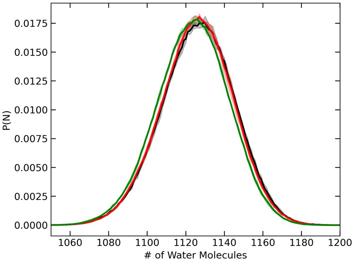
Probability distributions for the number of SPC/E water molecules calculated with GCMC/MD using Langevin dynamics with a 2 fs time step (green) or a 1 fs time step (red) or standard GCMC simulations at 510 K and chemical potential of −4.9037 kcal/mol (black). Solid lines correspond to averages over five independent replicas, while the shaded areas represent the standard deviations.

Gibbs ensemble MC provides a direct means for the calculation of vapor–liquid equilibria.⁴¹ In this method, two phases (liquid and vapor in this case) are simulated simultaneously. Equilibrium between the phases is achieved through MC moves that exchange volume and molecules between the phases, ensuring mechanical and chemical equilibrium. It has been suggested that the efficiency of the GEMC method could be improved by using an MC/MD approach (GEMC/MD), where MC moves are used for only the exchange of volume and molecules between the two phases while MD steps are used to sample conformational and configurational degrees of freedom.^42,90

GEMC/MD simulations were used to determine the vapor–liquid equilibria of SPC/E water at 300 K, 400 K, and 500 K. Simulations at 500 K were purposefully started far from equilibrium to observe the convergence behavior of the algorithm, which is shown in Figure 2. Similar data for the 400 and 300 K simulations are presented in Figure S3. Tabulated data for saturated liquid and vapor densities and vapor pressures are listed in Table 2. GEMC/MD results are in close agreement with data generated from standard GEMC simulations. Both the GEMC/MD and GEMC simulations at 500 K converge to the correct equilibrium densities, with the GEMC/MD simulations reaching equilibrium faster than the GEMC ones. Autocorrelation functions for −β(U_liq + U_vap) are presented in Figures S4–S6 for simulations at 300, 400, and 500 K, respectively. A correlation time analysis performed on −β(U_liq + U_vap) shows that the GEMC/MD approach reduced the correlation time by a factor of 3 to 4 compared with standard GEMC simulations, with the greatest improvement observed at 500 K. These results are consistent with the GCMC/MD and GCMC simulations, as shown in Table 2, where the molecule-transfer move is the primary limitation in sampling efficiency. The smaller improvement of GEMC/MD over GEMC at lower temperatures was expected, as the percentage of accepted molecule-transfer moves also decreases significantly under these conditions.

In summary, the MC/MD method produced uncorrelated data significantly faster than the standard MC method, as shown in Figures S1, S2, S4, S5, and S6. The normalized fluctuation autocorrelation functions produced from MC/MD simulations have significantly lower variance than those generated from MC simulations. These results show that for a given computational effort, more uncorrelated data were obtained with MC/MD simulations than with MC simulations.

Illustrative Applications: Graphene Slit Pore and BPTI.

Now that the ability of the hybrid workflow to produce correct results for simulations of bulk water has been demonstrated, two additional examples are presented to highlight the utility of the py-MCMD program.

In Figure 4, data are presented for simulations of water in a periodic rectangular box, partitioned into two separate compartments by two impermeable graphene sheets.¹⁹ In MD simulations, the inner region is not accessible because water cannot diffuse through the graphene layers; however, with the MC/MD approach and the intrabox swap moves, the entire simulation volume is accessible. Convergence of the density in each region was achieved in approximately 750 cycles, where each cycle comprised 1000 CD–CBMC intrabox swap moves and a 2 ps MD simulation. Additional simulations were performed using an unbiased single random trial position (simple MC) for the intrabox swap move to illustrate the impact of the CD–CMBC method on the efficiency of the MC/MD simulation. Simulations using an unbiased single random trial position required approximately 18 750 cycles to reach equilibrium. In this application, the computational cost of the CD–CBMC algorithm is approximately 25% larger than that of the simple MC algorithm.

Figure 4.

NVT simulations of water in a graphene slit pore. (A) Initial configuration. (B) Final configuration after the MC/MD simulation was performed. (C) Bulk water densities inside and outside the pore using CD–CBMC (black and blue) and simple MC (red and orange). Solid lines correspond to averages over five replicas, and the shaded areas represent standard deviations calculated from the five independent replicas.

Both approaches used here compare favorably with prior simulations of this system using the cavity-bias method, which required 50 000 cycles to reach equilibrium, where each cycle consisted of 25 000 MC trials and a 50 ps MD simulation.¹⁹ MC/MD simulations with CD–CBMC and simple MC intrabox swap moves required 66 and 2.6 times fewer cycles to reach equilibrium, respectively. Additionally the cycles used in this work were 25 times shorter than those used by Ben-Shalom et al.,¹⁹ further illustrating the significant improvement in sampling achieved with the CD–CBMC algorithm.

In the final example, GCMC/MD simulations were used to hydrate the buried binding pocket of bovine pancreatic trypsin inhibitor (BPTI), and the most probable water positions were compared with crystallographic data.⁶⁸ The binding pocket was defined as the region within 4.2 Å of the geometric center of the C_α atoms of the Tyr10 and Asn43 residues.²⁶ The average occupancy of each water site and the total number of observed water molecules within binding pocket are shown in Figure 5, while data for each replica are presented in Figures S7–S10. GCMC/MD simulations, initiated with an empty binding pocket, reached equilibrium (defined as an occupancy of ≥0.75) within 0.3 ns, while MD simulations took approximately 2.7 ns to fill all three water sites. Running on four cores of an Intel E5–2630v4 CPU and an NVIDIA RTX 2080TI GPU, the GCMC/MD simulations were 1.8 times (total CPU + GPU computational time) slower than MD simulations. Considering the significant reduction in the time scale required to fully hydrate the binding pocket, the GCMC/MD simulations produced a computational efficiency approximately 5 times better than that of the MD simulations.

Figure 5.

Hydration of a buried binding pocket in BPTI. (A) Comparison of crystallographic water locations⁶⁸ (cyan) with average water locations predicted from GCMC/MD simulations (red). Any water positions that were observed less than 40% of the time have been omitted for clarity. (B) Times required for GCMC/MD simulations (black) and MD simulations (red) to fill water sites in the binding pocket. The average occupancy for each water site is shown as an average over water occupancies during 0.1 ns of simulation. The total number of water molecules in the pocket was calculated by counting oxygen atoms within 4.2 Å of the geometric center of the C_α atoms of Tyr10 and Asn43. Solid lines correspond to averages over 10 independent simulations, while the shaded areas represent the standard deviations. Data for each replica are presented in Figures S7–S10.

Average water positions within the binding pocket were calculated to be within 0.38 Å of experiment,⁶⁸ as shown in Figure 5. The agreement with experiment is slightly better in this work than in Samways et al.,²⁶ whose results were within 0.6 Å of experiment. The difference may be due to the choice of force field: in the study by Samways et al., calculations were performed with the AMBER ff14sb force field⁹¹ for BPTI and the original TIP3P force field⁹² for water, while in this work, CHARMM36 was used for BPTI and mTIP3P⁷⁴ for water.

To understand the dynamics of hydration of the BPTI binding pocket, fluctuations of the random coil between the α-helix and the β-sheet (residues 36–47) were calculated with respect to the crystallographic structure for a system with a dehydrated binding pocket. The backbone of residues 36–47 was clustered using the quality threshold (QT) algorithm⁹³ as implemented in VMD.⁷³ Figure 6 shows the top three random coil clusters for the first 2 ns of one MD simulation. The random coil was collapsed for the majority of the first 2 ns of the MD simulation (green lines in Figure 6A), which blocked water from entering Site 1 of the binding pocket. Site 1 became accessible only when a random fluctuation of the coil resulted in opening of the pocket. On the other hand, the GCMC/MD approach rapidly hydrated the binding pocket, especially Site 1, preventing the collapse of the binding pocket and enabling further hydration through diffusion of surrounding waters in addition to molecule transfers via GCMC/MD. An example of random coil behavior for the dehydrated binding pocket in the MD simulation is provided in Movie S1.

Figure 6.

Effect of hydration on binding pocket stability in BPTI given by representative single MC/MD and MD simulations. (A) Comparison of the crystallographic structure⁶⁸ (purple) with the MD simulation (green). The green, yellow, and orange lines represent the top three random coil (residues 36–47) clusters within the first 2 ns of MD simulation, which block the crystallographic water sites. (B) The 50 ps running averages of RMSD calculations of the protein’s backbone for residues 36–47 with respect to the reference crystallographic structure⁶⁸ for the MC/MD (black) and MD (red) simulations. (C) The 50 ps running averages of the total number of observed waters within the binding pocket for the MC/MD (black) and MD (red) simulations. Individual replicas are presented in Figure S11. The binding pocket is defined as a sphere of radius 4.2 Å centered at the geometric center of the C_α atoms of Tyr10 and Asn43.

Subtle differences were observed between the MD and GCMC/MD simulations in the stability of the fully hydrated BPTI binding pocket. Figure 6 shows the root-mean-square deviation (RMSD) values of residues 36–47 with respect to the crystallographic structure for one trajectory generated from MD or GCMC/MD simulations after the backbone of residues in α-helices and β-sheets (residues 3–6, 18–24, 29–35, and 48–55) were aligned with the crystallographic structure. Plots showing fluctuations of the random coil for each of the 10 replicas of MD and GCMC/MD simulations are provided in Figure S11. During the first 2 ns of the MD simulation, the binding pocket was dehydrated, and large fluctuations in the random coil were observed. After the binding pocket was fully hydrated, fluctuations in the RMSD decreased from 1.6 Å to an average of 0.7 Å. On the other hand, GCMC/MD simulations produced larger RMSD values (approximately 1.0 Å) despite achieving full hydration of the binding pocket significantly faster than MD simulations. The larger fluctuations observed in the random coil may be due to the assignment of random velocities (from a Maxwell–Boltzmann distribution^48,49) to newly inserted water molecules. If maintaining correct protein dynamics is important, this issue could be mitigated by increasing the length of the MD component of each cycle, reducing the number of attempted water molecule transfers during the simulation.

CONCLUSION

py-MCMD allows users to alter most of the parameters governing a simulation’s behavior, and the strategy of linking two existing simulation engines, GOMC and NAMD, with an external Python script provides tremendous flexibility. With this approach, MD configurational sampling can be incorporated into Monte Carlo simulations in any ensemble supported by GOMC. Additionally, Monte Carlo moves may be integrated into any equilibrium NVT or NPT MD simulation. It is also possible to develop new sampling strategies with minor revisions to py-MCMD, using a combination of MC to propose trial configurations and nonequilibrium MD for relaxation of the local structure.^23,94

Predictions of the hybrid MC/MD simulations of bulk SPC/E water performed with py-MCMD were in close agreement with reference MC simulations. Substantial gains in computational efficiency were observed for the MC/MD approach compared with MC, ranging from a 2-fold improvement for GCMC/MD simulations at 510 K to a 136-fold improvement for NPT simulations at 298 K. NVT MC/MD simulations with an intrabox swap move were used to rapidly equilibrate the density of water in a system containing a graphene slit pore. The coupled–decoupled configurational-bias Monte Carlo (CD–CBMC) algorithm³⁷ substantially improved the sampling efficiency for the transfer of water molecules. MC/MD simulations using CD–CBMC required 25 times fewer cycles to reach equilibrium than MC/MD simulations using an unbiased single random trial position, with a modest 25% increase in computational cost, and 66 times fewer cycles than prior hybrid simulations that used the cavity-bias method.¹⁹

Finally, GCMC/MD simulations used to hydrate a buried binding pocket in BPTI demonstrated a 5-fold improvement in computational efficiency compared with MD simulations, and the water molecule locations observed in the GCMC/MD simulations were within 0.38 Å of the crystallographic water sites. However, subtle differences were observed in protein dynamics in MD and GCMC/MD simulations. The GCMC/MD simulations exhibited larger fluctuations of the random coil (residues 36–47) than the MD simulations, which we attribute to velocity initialization of inserted water in the GCMC/MD simulations to random values drawn from a Maxwell–Boltzmann distribution. It is expected that these differences could be addressed by increasing the length of the MD component of each cycle in the GCMC/MD simulation.

As an MC engine, GOMC includes a number of advanced configurational-bias algorithms that support the insertion of molecules having more complex topologies with acceptance rates that are 1–2 orders of magnitude greater than those of naive approaches.^37–40 While the examples provided here focused on water, it is straightforward to perform similar calculations with larger, more complex molecules⁴⁰ without modification of the software. In addition to the applications provided here, py-MCMD could be used to simulate other phenomena, such as diffusion¹⁶ or gas adsorption in polymers.⁹⁰

REFERENCES

- (1).Phillips JC; Hardy DJ; Maia JDC; Stone JE; Ribeiro JV; Bernardi RC; Buch R; Fiorin G; Hénin J; Jiang W; McGreevy R; Melo MCR; Radak B; Skeel RD; Singharoy A; Wang Y; Roux B; Aksimentiev A; Luthey-Schulten Z; Kalé LV; Schulten K; Chipot C; Tajkhorshid E Scalable molecular dynamics on CPU and GPU architectures with NAMD. J. Chem. Phys. 2020, 153, 044130. [DOI] [PMC free article] [PubMed] [Google Scholar]
- (2).Enkavi G; Javanainen M; Kulig W; Róg T; Vattulainen I Multiscale Simulations of Biological Membranes: The Challenge To Understand Biological Phenomena in a Living Substance. Chem. Rev. 2019, 119, 5607–5774. [DOI] [PMC free article] [PubMed] [Google Scholar]
- (3).Bochicchio A; Brandner AF; Engberg O; Huster D; Böckmann RA Spontaneous membrane nanodomain formation in the absence or presence of the neurotransmitter serotonin. Front. Cell Dev. Biol. 2020, 8, 601145. [DOI] [PMC free article] [PubMed] [Google Scholar]
- (4).Durrant JD; McCammon JA Molecular dynamics simulations and drug discovery. BMC Biol 2011, 9, No. 71. [DOI] [PMC free article] [PubMed] [Google Scholar]
- (5).De Vivo M; Masetti M; Bottegoni G; Cavalli A Role of molecular dynamics and related methods in drug discovery. J. Med. Chem. 2016, 59, 4035–4061. [DOI] [PubMed] [Google Scholar]
- (6).Wang L; Wu Y; Deng Y; Kim B; Pierce L; Krilov G; Lupyan D; Robinson S; Dahlgren MK; Greenwood J; Romero DL; Masse C; Knight JL; Steinbrecher T; Beuming T; Damm W; Harder E; Sherman W; Brewer M; Wester R; Murcko M; Frye L; Farid R; Lin T; Mobley DL; Jorgensen WL; Berne BJ; Friesner RA; Abel R Accurate and Reliable Prediction of Relative Ligand Binding Potency in Prospective Drug Discovery by Way of a Modern Free-Energy Calculation Protocol and Force Field. J. Am. Chem. Soc. 2015, 137, 2695–2703. [DOI] [PubMed] [Google Scholar]
- (7).Klauda JB; Venable RM; Freites JA; O’Connor JW; Tobias DJ; Mondragon-Ramirez C; Vorobyov I; MacKerell AD Jr.; Pastor RW Update of the CHARMM All-Atom Additive Force Field for Lipids: Validation on Six Lipid Types. J. Phys. Chem. B 2010, 114, 7830–7843. [DOI] [PMC free article] [PubMed] [Google Scholar]
- (8).Venable RM; Brown FL; Pastor RW Mechanical properties of lipid bilayers from molecular dynamics simulation. Chem. Phys. Lipids 2015, 192, 60–74. [DOI] [PMC free article] [PubMed] [Google Scholar]
- (9).Muller MP; Jiang T; Sun C; Lihan M; Pant S; Mahinthichaichan P; Trifan A; Tajkhorshid E Characterization of Lipid–Protein Interactions and Lipid-Mediated Modulation of Membrane Protein Function through Molecular Simulations. Chem. Rev. 2019, 119, 6086–6161. [DOI] [PMC free article] [PubMed] [Google Scholar]
- (10).Jiang T; Wen P-C; Trebesch N; Zhao Z; Pant S; Kapoor K; Shekhar M; Tajkhorshid E Computational Dissection of Membrane Transport at a Microscopic Level. Trends Biochem. Sci. 2020, 45, 202–216. [DOI] [PMC free article] [PubMed] [Google Scholar]
- (11).Karplus M; Kuriyan J Molecular dynamics and protein function. Proc. Natl. Acad. Sci. U.S.A. 2005, 102, 6679–6685. [DOI] [PMC free article] [PubMed] [Google Scholar]
- (12).Sharma S; Lindau M Molecular mechanism of fusion pore formation driven by the neuronal SNARE complex. Proc. Natl. Acad. Sci. U.S.A. 2018, 115, 12751–12756. [DOI] [PMC free article] [PubMed] [Google Scholar]
- (13).Bendahmane M; Bohannon KP; Bradberry MM; Rao TC; Schmidtke MW; Abbineni PS; Chon NL; Tran S; Lin H; Chapman ER; Knight JD; Anantharam A The synaptotagmin C2B domain calcium-binding loops modulate the rate of fusion pore expansion. Mol. Biol. Cell 2018, 29, 834–845. [DOI] [PMC free article] [PubMed] [Google Scholar]
- (14).Lee EH; Hsin J; Sotomayor M; Comellas G; Schulten K Discovery Through the Computational Microscope. Structure 2009, 17, 1295–1306. [DOI] [PMC free article] [PubMed] [Google Scholar]
- (15).Dror RO; Dirks RM; Grossman J; Xu H; Shaw DE Biomolecular Simulation: A Computational Microscope for Molecular Biology. Annu. Rev. Biophys. 2012, 41, 429–452. [DOI] [PubMed] [Google Scholar]
- (16).Heffelfinger GS; van Swol F Diffusion in Lennard-Jones fluids using dual control volume grand canonical molecular dynamics simulation (DCV-GCMD). J. Chem. Phys. 1994, 100, 7548–7552. [Google Scholar]
- (17).Woo HJ; Dinner AR; Roux B Grand canonical Monte Carlo simulations of water in protein environments. J. Chem. Phys. 2004, 121, 6392–6400. [DOI] [PubMed] [Google Scholar]
- (18).Henry RM; Yu CH; Rodinger T; Pomès R. Functional hydration and conformational gating of proton uptake in cytochrome c oxidase. J. Mol. Biol. 2009, 387, 1165–1185. [DOI] [PubMed] [Google Scholar]
- (19).Ben-Shalom IY; Lin C; Kurtzman T; Walker RC; Gilson MK Simulating water exchange to buried binding sites. J. Chem. Theory Comput. 2019, 15, 2684–2691. [DOI] [PMC free article] [PubMed] [Google Scholar]
- (20).Bodnarchuk MS; Packer MJ; Haywood A Utilizing grand canonical Monte Carlo methods in drug discovery. ACS Med. Chem. Lett. 2020, 11, 77–82. [DOI] [PMC free article] [PubMed] [Google Scholar]
- (21).Ross GA; Russell E; Deng Y; Lu C; Harder ED; Abel R; Wang L Enhancing water sampling in free energy calculations with grand canonical Monte Carlo. J. Chem. Theory Comput. 2020, 16, 6061–6076. [DOI] [PubMed] [Google Scholar]
- (22).De Joannis J; Coppock PS; Yin F; Mori M; Zamorano A; Kindt JT Atomistic simulation of cholesterol effects on miscibility of saturated and unsaturated phospholipids: implications for liquid-ordered/liquid-disordered phase coexistence. J. Am. Chem. Soc. 2011, 133, 3625–3634. [DOI] [PubMed] [Google Scholar]
- (23).Fathizadeh A; Elber R A Mixed Alchemical and Equilibrium Dynamics to Simulate Heterogeneous Dense Fluids: Illustrations for Lennard-Jones Mixtures and Phospholipid Membranes. J. Chem. Phys. 2018, 149, 072325. [DOI] [PMC free article] [PubMed] [Google Scholar]
- (24).Deng Y; Roux B Computation of binding free energy with molecular dynamics and grand canonical Monte Carlo simulations. J. Chem. Phys. 2008, 128, 115103. [DOI] [PubMed] [Google Scholar]
- (25).Pool R; Heringa J; Hoefling M; Schulz R; Smith JC; Feenstra KA Enabling grand-canonical Monte Carlo: extending the flexibility of GROMACS through the grompy Python interface module. J. Comput. Chem. 2012, 33, 1207–1214. [DOI] [PubMed] [Google Scholar]
- (26).Samways ML; Bruce Macdonald HE; Essex JW grand: a Python module for grand canonical water sampling in OpenMM. J. Chem. Inf. Model. 2020, 60, 4436–4441. [DOI] [PubMed] [Google Scholar]
- (27).Wahl J; Smieško M Assessing the predictive power of relative binding free energy calculations for test cases involving displacement of binding site water molecules. J. Chem. Inf. Model. 2019, 59, 754–765. [DOI] [PubMed] [Google Scholar]
- (28).Ben-Shalom IY; Lin Z; Radak BK; Lin C; Sherman W; Gilson MK Accounting for the central role of interfacial water in protein-ligand binding free energy calculations. J. Chem. Theory Comput. 2020, 16, 7883–7894. [DOI] [PMC free article] [PubMed] [Google Scholar]
- (29).Im W; Seefeld S; Roux B A Grand Canonical Monte Carlo-Brownian Dynamics Algorithm for Simulating Ion Channels. Biophys. J. 2000, 79, 788–801. [DOI] [PMC free article] [PubMed] [Google Scholar]
- (30).Solano CJ; Prajapati JD; Pothula KR; Kleinekathöfer U Brownian dynamics approach including explicit atoms for studying ion permeation and substrate translocation across nanopores. J. Chem. Theory Comput. 2018, 14, 6701–6713. [DOI] [PubMed] [Google Scholar]
- (31).Hu J; Ma A; Dinner AR Monte Carlo simulations of biomolecules: the MC module in CHARMM. J. Comput. Chem. 2006, 27, 203–216. [DOI] [PubMed] [Google Scholar]
- (32).Plimpton SJ Fast parallel algorithms for short-range molecular dynamics. J. Comput. Phys. 1995, 117, 1–19. [Google Scholar]
- (33).Eastman P; Swails J; Chodera JD; McGibbon RT; Zhao Y; Beauchamp KA; Wang L-P; Simmonett AC; Harrigan MP; Stern CD; Wiewiora RP; Brooks BR; Pande VS OpenMM 7: Rapid development of high performance algorithms for molecular dynamics. PLoS Comput. Biol. 2017, 13, No. e1005659. [DOI] [PMC free article] [PubMed] [Google Scholar]
- (34).Chodera J; Rizzi A; Naden L; Beauchamp K; Grinaway P; Fass J; Wade A; Rustenburg B; Ross GA; Krämer A; Macdonald HB; Rodríguez-Guerra J; dominicrufa; Simmonett A; Swenson DW; Henry M; Roet S; Silveira A choderalab/openmmtools: 0.20.3 Bugfix Release, 2021. DOI: 10.5281/zenodo.4639586. [DOI] [Google Scholar]
- (35).Mezei M A cavity-biased (T, V, μ) Monte Carlo method for the computer simulation of fluids. Mol. Phys. 1980, 40, 901–906. [Google Scholar]
- (36).Crawford B; Potoff J py-MCMD: A Python Library for Performing Hybrid Monte Carlo/Molecular Dynamics Simulations with GOMC and NAMD. https://github.com/GOMC-WSU/py-MCMD (accessed January 2022). [DOI] [PMC free article] [PubMed]
- (37).Martin M; Siepmann J Novel configurational-bias Monte Carlo method for branched molecules. Transferable potentials for phase equilibria. 2. United-atom description of branched alkanes. J. Phys. Chem. B 1999, 103, 4508–4517. [Google Scholar]
- (38).Soroush Barhaghi M; Torabi K; Nejahi Y; Schwiebert L; Potoff JJ Molecular exchange Monte Carlo: a generalized method for identity exchanges in grand canonical Monte Carlo simulations. J. Chem. Phys. 2018, 149, 072318. [DOI] [PubMed] [Google Scholar]
- (39).Soroush Barhaghi M; Potoff JJ Prediction of phase equilibria and Gibbs free energies of transfer using molecular exchange Monte Carlo in the Gibbs ensemble. Fluid Phase Equilib. 2019, 486, 106–118. [Google Scholar]
- (40).Nejahi Y; Barhaghi MS; Schwing G; Schwiebert L; Potoff J Update 2.70 to “GOMC: GPU optimized Monte Carlo for the simulation of phase equilibria and physical properties of complex fluids”. SoftwareX 2021, 13, 100627. [Google Scholar]
- (41).Panagiotopoulos AZ; Quirke N; Stapleton M; Tildesley DJ Phase equilibria by simulation in the Gibbs ensemble alternative derivation, generalization and application to mixture and membrane equilibria. Mol. Phys. 1988, 63, 527–545. [Google Scholar]
- (42).Gartner TE; Epps TH; Jayaraman A Leveraging Gibbs Ensemble Molecular Dynamics and Hybrid Monte Carlo/Molecular Dynamics for Efficient Study of Phase Equilibria. J. Chem. Theory Comput 2016, 12, 5501–5510. [DOI] [PubMed] [Google Scholar]
- (43).Fass J; Sivak DA; Crooks GE; Beauchamp KA; Leimkuhler B; Chodera JD Quantifying Configuration-Sampling Error in Langevin Simulations of Complex Molecular Systems. Entropy 2018, 20, No. 318. [DOI] [PMC free article] [PubMed] [Google Scholar]
- (44).Bruünger A; Brooks CB III; Karplus M Stochastic boundary-conditions for molecular dynamics simulations of ST2 water. Chem. Phys. Lett. 1984, 105, 495–500. [Google Scholar]
- (45).Leimkuhler B; Matthews C Robust and efficient configurational molecular sampling via Langevin dynamics. J. Chem. Phys. 2013, 138, No. 174102. [DOI] [PubMed] [Google Scholar]
- (46).Leimkuhler B; Matthews C Efficient molecular dynamics using geodesic integration and solvent–solute splitting. Proc. R. Soc. A 2016, 472, No. 20160138. [DOI] [PMC free article] [PubMed] [Google Scholar]
- (47).Leimkuhler B; Matthews C Rational Construction of Stochastic Numerical Methods for Molecular Sampling. Appl. Math. Res. eXpress 2012, 2013, 34–56. [Google Scholar]
- (48).Boltzmann L Weitere studien uüber das Wärmegleichgewicht unter gasmolekuülen. Sitzungsber. Kaiserl. Akad. Wiss., Math.-Naturwiss. Cl. 1872, 66, 275–370. [Google Scholar]
- (49).Maxwell MA; J CV Illustrations of the dynamical theory of gases.—Part I. On the motions and collisions of perfectly elastic spheres. London Edinburgh Philos. Mag. J. Sci. 1860, 19, 19–32. [Google Scholar]
- (50).Allen MP; Tildesley DJ Computer Simulation of Liquids; Oxford University Press: New York, 1987. [Google Scholar]
- (51).Ewald PP Die Berechnung optischer und elektrostatischer Gitterpotentiale. Ann. Phys. 1921, 369, 253–287. [Google Scholar]
- (52).Darden T; York D; Pedersen L Particle Mesh Ewald: an N·log(N) Method for Ewald Sums in Large Systems. J. Chem. Phys. 1993, 98, 10089–10092. [Google Scholar]
- (53).Essmann U; Perera L; Berkowitz ML; Darden T; Lee H; Pedersen LG A smooth particle mesh Ewald method. J. Chem. Phys. 1995, 103, 8577–8593. [Google Scholar]
- (54).Bai P; Siepmann JI Assessment and optimization of configurational-bias Monte Carlo particle swap strategies for simulations of water in the Gibbs ensemble. J. Chem. Theory Comput. 2017, 13, 431–440. [DOI] [PubMed] [Google Scholar]
- (55).Shah JK; Maginn EJ A general and efficient Monte Carlo method for sampling intramolecular degrees of freedom of branched and cyclic molecules. J. Chem. Phys. 2011, 135, 134121. [DOI] [PubMed] [Google Scholar]
- (56).Miyamoto S; Kollman PA Settle: an analytical version of the SHAKE and RATTLE algorithm for rigid water molecules. J. Comput. Chem. 1992, 13, 952–962. [Google Scholar]
- (57).Schneider T; Stoll E Molecular-dynamics study of a three-dimensional one-component model for distortive phase transitions. Phys. Rev. B 1978, 17, 1302–1322. [Google Scholar]
- (58).Tuckerman M; Berne BJ; Martyna GJ Reversible multiple time scale molecular dynamics. J. Chem. Phys. 1992, 97, 1990–2001. [Google Scholar]
- (59).Berendsen HJC; Grigera JR; Straatsma TP The Missing Term in Effective Pair Potentials. J. Phys. Chem. 1987, 91, 6269–6271. [Google Scholar]
- (60).Summers AZ; Gilmer JB; Iacovella CR; Cummings PT; McCabe C MoSDeF, a Python framework enabling large-scale computational screening of soft matter: application to chemistry-property relationships in lubricating monolayer films. J. Chem. Theory Comput. 2020, 16, 1779–1793. [DOI] [PubMed] [Google Scholar]
- (61).Klein C; Summers AZ; Thompson MW; Gilmer JB; McCabe C; Cummings PT; Sallai J; Iacovella CR Formalizing atom-typing and the dissemination of force fields with foyer. Comput. Mater. Sci. 2019, 167, 215–227. [Google Scholar]
- (62).Thompson MW; Gilmer JB; Matsumoto RA; Quach CD; Shamaprasad P; Yang AH; Iacovella CR; McCabe C; Cummings PT Towards molecular simulations that are transparent, reproducible, usable by others, and extensible (TRUE). Mol. Phys. 2020, 118, No. e1742938. [DOI] [PMC free article] [PubMed] [Google Scholar]
- (63).Matsumoto R; Thompson M; DeFever R Pore-builder. https://github.com/rmatsum836/Pore-Builder (accessed March 2021).
- (64).Nejahi Y; Soroush Barhaghi M; Mick J; Jackman B; Rushaidat K; Li Y; Schwiebert L; Potoff J “GOMC: GPU optimized Monte Carlo for the simulation of phase equilibria and physical properties of complex fluids”. SoftwareX 2019, 9, 20–27. [Google Scholar]
- (65).Shirts MR; Chodera JD Statistically optimal analysis of samples from multiple equilibrium states. J. Chem. Phys. 2008, 129, 124105. [DOI] [PMC free article] [PubMed] [Google Scholar]
- (66).Chodera JD; Swope WC; Pitera JW; Seok C; Dill KA Use of the Weighted Histogram Analysis Method for the Analysis of Simulated and Parallel Tempering Simulations. J. Chem. Theory Comput. 2007, 3, 26–41. [DOI] [PubMed] [Google Scholar]
- (67).Striolo A; Chialvo AA; Cummings PT; Gubbins KE Water adsorption in carbon-slit nanopores. Langmuir 2003, 19, 8583–8591. [Google Scholar]
- (68).Wlodawer A; Walter J; Huber R; Sjölin L Structure of bovine pancreatic trypsin inhibitor: results of joint neutron and X-ray refinement of crystal form II. J. Mol. Biol. 1984, 180, 301–329. [DOI] [PubMed] [Google Scholar]
- (69).Burley SK; Bhikadiya C; Bi C; Bittrich S; Chen L; Crichlow GV; Christie CH; Dalenberg K; Di Costanzo L; Duarte JM; Dutta S; Feng Z; Ganesan S; Goodsell DS; Ghosh S; Green RK; Guranović V; Guzenko D; Hudson BP; Lawson CL; Liang Y; Lowe R; Namkoong H; Peisach E; Persikova I; Randle C; Rose A; Rose Y; Sali A; Segura J; Sekharan M; Shao C; Tao Y-P; Voigt M; Westbrook JD; Young JY; Zardecki C; Zhuravleva M RCSB Protein Data Bank: powerful new tools for exploring 3D structures of biological macromolecules for basic and applied research and education in fundamental biology, biomedicine, biotechnology, bioengineering and energy sciences. Nucleic Acids Res. 2021, 49, D437–D451. [DOI] [PMC free article] [PubMed] [Google Scholar]
- (70).Berman HM; Westbrook J; Feng Z; Gilliland G; Bhat TN; Weissig H; Shindyalov IN; Bourne PE The Protein Data Bank. Nucleic Acids Res. 2000, 28, 235–242. [DOI] [PMC free article] [PubMed] [Google Scholar]
- (71).Berman H; Henrick K; Nakamura H Announcing the worldwide Protein Data Bank. Nat. Struct. Biol. 2003, 10, 980. [DOI] [PubMed] [Google Scholar]
- (72).Ribeiro JV; Bernardi RC; Rudack T; Stone JE; Phillips JC; Freddolino PL; Schulten K QwikMD-Integrative Molecular Dynamics Toolkit for Novices and Experts. Sci. Rep. 2016, 6, 26536. [DOI] [PMC free article] [PubMed] [Google Scholar]
- (73).Humphrey W; Dalke A; Schulten K VMD – Visual Molecular Dynamics. J. Mol. Graphics 1996, 14, 33–38. [DOI] [PubMed] [Google Scholar]
- (74).MacKerell AD Jr.; Bashford D; Bellott M; Dunbrack RL Jr.; Evanseck JD; Field MJ; Fischer S; Gao J; Guo H; Ha S; Joseph-McCarthy D; Kuchnir L; Kuczera K; Lau FTK; Mattos C; Michnick S; Ngo T; Nguyen DT; Prodhom B; Reiher IWE; Roux B; Schlenkrich M; Smith J; Stote R; Straub J; Watanabe M; Wiorkiewicz-Kuczera J; Yin D; Karplus M All-atom empirical potential for molecular modeling and dynamics studies of proteins. J. Phys. Chem. B 1998, 102, 3586–3616. [DOI] [PubMed] [Google Scholar]
- (75).Brooks BR; Brooks CL; Mackerell AD; Nilsson L; Petrella RJ; Roux B; Won Y; Archontis G; Bartels C; Boresch S; Caflisch A; Caves L; Cui Q; Dinner AR; Feig M; Fischer S; Gao J; Hodoscek M; Im W; Kuczera K; Lazaridis T; Ma J; Ovchinnikov V; Paci E; Pastor RW; Post CB; Pu JZ; Schaefer M; Tidor B; Venable RM; Woodcock HL; Wu X; Yang W; York DM; Karplus M CHARMM: The biomolecular simulation program. J. Comput. Chem. 2009, 30, 1545–1614. [DOI] [PMC free article] [PubMed] [Google Scholar]
- (76).Jo S; Kim T; Iyer VG; Im W CHARMM-GUI: a Web-based Graphical User Interface for CHARMM. J. Comput. Chem. 2008, 29, 1859–1865. [DOI] [PubMed] [Google Scholar]
- (77).Brooks BR; Bruccoleri RE; Olafson BD; States DJ; Swaminathan S; Karplus M CHARMM: A Program for Macromolecular Energy, Minimization, and Dynamics Calculations. J. Comput. Chem. 1983, 4, 187–217. [Google Scholar]
- (78).Best RB; Zhu X; Shim J; Lopes PEM; Mittal J; Feig M; MacKerell AD Optimization of the additive CHARMM all-atom protein force field targeting improved sampling of the backbone ϕ, ψ and side-chain χ1 and χ2 dihedral angles. J. Chem. Theory Comput. 2012, 8, 3257–3273. [DOI] [PMC free article] [PubMed] [Google Scholar]
- (79).Lee S; Tran A; Allsopp M; Lim JB; Hénin J; Klauda JB CHARMM36 United Atom Chain Model for Lipids and Surfactants. J. Phys. Chem. B 2014, 118, 547–556. [DOI] [PubMed] [Google Scholar]
- (80).Huang J; MacKerell AD CHARMM36 all-atom additive protein force field: Validation based on comparison to NMR data. J. Comput. Chem. 2013, 34, 2135–2145. [DOI] [PMC free article] [PubMed] [Google Scholar]
- (81).Lee J; Cheng X; Swails JM; Yeom M; Eastman PK; Lemkul JA; Wei S; Buckner J; Jeong J; Qi Y; Jo S; Pande VS; Case DA; Brooks CL III; MacKerell AD Jr.; Klauda JB; Im W CHARMM-GUI Input Generator for NAMD, GROMACS, AMBER, OpenMM, and CHARMM/OpenMM Simulations Using the CHARMM36 Additive Force Field. J. Chem. Theory Comput. 2016, 12, 405–413. [DOI] [PMC free article] [PubMed] [Google Scholar]
- (82).Huang J; Rauscher S; Nawrocki G; Ran T; Feig M; de Groot BL; Grubmuüller, H.; MacKerell, A. D., Jr CHARMM36m: an improved force field for folded and intrinsically disordered proteins. Nat. Methods 2017, 14, 71–73. [DOI] [PMC free article] [PubMed] [Google Scholar]
- (83).Boonstra S; Onck PR; van der Giessen E CHARMM TIP3P water model suppresses peptide folding by solvating the unfolded state. J. Phys. Chem. B 2016, 120, 3692–3698. [DOI] [PubMed] [Google Scholar]
- (84).Feller SE; Zhang Y; Pastor RW; Brooks BR Constant pressure molecular dynamics simulation: The Langevin piston method. J. Chem. Phys. 1995, 103, 4613–4621. [Google Scholar]
- (85).Hoover WG Canonical Dynamics: Equilibrium Phase-Space Distributions. Phys. Rev. A 1985, 31, 1695–1697. [DOI] [PubMed] [Google Scholar]
- (86).Hoover WG Constant-Pressure Equations of Motion. Phys. Rev. A 1986, 34, 2499–2500. [DOI] [PubMed] [Google Scholar]
- (87).Ong EE; Liow J-L The temperature-dependent structure, hydrogen bonding and other related dynamic properties of the standard TIP3P and CHARMM-modified TIP3P water models. Fluid Phase Equilib. 2019, 481, 55–65. [Google Scholar]
- (88).Sakamaki R; Sum AK; Narumi T; Yasuoka K Molecular dynamics simulations of vapor/liquid coexistence using the non-polarizable water models. J. Chem. Phys. 2011, 134, 124708. [DOI] [PubMed] [Google Scholar]
- (89).Boulougouris GC; Economou IG; Theodorou DN Engineering a molecular model for water phase equilibrium over a wide temperature range. J. Phys. Chem. B 1998, 102, 1029–1035. [Google Scholar]
- (90).Gartner TE; Jayaraman A Macromolecular ‘size’ and ‘hardness’ drives structure in solvent-swollen blends of linear, cyclic, and star polymers. Soft Matter 2018, 14, 411–423. [DOI] [PubMed] [Google Scholar]
- (91).Maier JA; Martinez C; Kasavajhala K; Wickstrom L; Hauser KE; Simmerling C ff14SB: Improving the Accuracy of Protein Side Chain and Backbone Parameters from ff99SB. J. Chem. Theory Comput. 2015, 11, 3696–3713. [DOI] [PMC free article] [PubMed] [Google Scholar]
- (92).Jorgensen W; Chandrasekhar J; Madura JD; Impey RW; Klein ML Comparison of Simple Potential Functions for Simulating Liquid Water. J. Chem. Phys. 1983, 79, 926–935. [Google Scholar]
- (93).Heyer LJ; Kruglyak S; Yooseph S Exploring expression data: identification and analysis of coexpressed genes. Gen. Res. 1999, 9, 1106–1115. [DOI] [PMC free article] [PubMed] [Google Scholar]
- (94).Chen Y; Roux B Generalized Metropolis Acceptance Criterion for Hybrid Non-equilibrium Molecular Dynamics–Monte Carlo Simulations. J. Chem. Phys. 2015, 142, 024101. [DOI] [PubMed] [Google Scholar]
Associated Data
This section collects any data citations, data availability statements, or supplementary materials included in this article.