It’s all relative: Regression analysis with compositional predictors

Abstract

Compositional data reside in a simplex and measure fractions or proportions of parts to a whole. Most existing regression methods for such data rely on log-ratio transformations that are inadequate or inappropriate in modeling high-dimensional data with excessive zeros and hierarchical structures. Moreover, such models usually lack a straightforward interpretation due to the interrelation between parts of a composition. We develop a novel relative-shift regression framework that directly uses proportions as predictors. The new framework provides a paradigm shift for regression analysis with compositional predictors and offers a superior interpretation of how shifting concentration between parts affects the response. New equi-sparsity and tree-guided regularization methods and an efficient smoothing proximal gradient algorithm are developed to facilitate feature aggregation and dimension reduction in regression. A unified finite-sample prediction error bound is derived for the proposed regularized estimators. We demonstrate the efficacy of the proposed methods in extensive simulation studies and a real gut microbiome study. Guided by the taxonomy of the microbiome data, the framework identifies important taxa at different taxonomic levels associated with the neurodevelopment of preterm infants.

1 |. INTRODUCTION

Compositional data characterize fractions or proportions of a whole and contain relative information. Such data are ubiquitous in various disciplines, such as chemistry, geology, ecology, and microbiology. Proportions are strictly nonnegative, bounded, and subject to a unit-sum constraint. As compositional data reside in a simplex, many standard notions and statistical methods do not directly apply (Aitchison, 1982). In addition, compositional data can be high-dimensional, inflated with excessive zeros, and organized in a hierarchical tree structure.

For instance, in microbiome studies, data are typically measured through high-throughput sequencing technology (e.g., 16S rRNA sequencing) and normalized as compositions due to heterogeneous library sizes between samples (Gloor et al., 2016; Tsilimigras & Fodor, 2016). The number of features (known as operational taxonomic units [OTUs], or taxa) may far exceed the number of samples. Since not all OTUs are present or detected in all samples, microbiome data are usually highly sparse with few dominant parts and excessive zeros (Xia et al., 2018; Xu et al., 2021). In addition, there also exists a hierarchical tree structure among OTUs that captures the taxonomy of the microbes (Silverman et al., 2017). Such hierarchical structure is important because OTU data at lower taxonomic ranks have higher resolution (i.e., more features) but are more prone to measurement errors, while data at higher taxonomic ranks have lower resolution with higher accuracy. There is a trade-off between data resolution and accuracy along the taxonomic hierarchy, which should be carefully taken into account in statistical analysis.

The unique features of compositional data pose new challenges for statistical analysis (Aitchison & Egozcue, 2005; Li, 2015). In this paper, we focus on the regression analysis with compositional predictors. Existing methods typically transform compositional data via log-ratios first (i.e., Aitchison’s approach, Aitchison, 1983) before further analyses. Subsequently, linear regression models are built upon transformed data. For example, one of the most commonly used models is the log-contrast model (Aitchison & Bacon-Shone, 1984) where log-ratio-transformed proportions are used as predictors in a linear regression. An equivalent symmetric form of the model is y = β₀ + β₁ log x₁ + ⋯ + β_p log x_p + ε, where the compositional vector x is nonzero and resides in the (p − 1)-simplex ${\mathbb{S}}^{p-1}=\left\{x={\left(x_1,\dots ,x_p\right)}^T\in {ℝ}^p:{\sum }_{j=1}^p{x}_j=1,x_j\ge 0,j=1,\dots ,p\right\}$ and the coefficients satisfy a linear constraint ${\sum }_{j=1}^p{\beta }_j=0$. The model enjoys the subcompositional coherence and scale and permutation invariance properties (Aitchison, 1982). Lin et al. (2014) and Shi et al. (2016) further proposed variable selection methods for such models to handle high-dimensional data. Centered log-ratio transformation is also frequently used in the literature and it has been shown to be equivalent to the log-contrast model if the zero-sum constraint is imposed on the regression coefficients (Wang & Zhao, 2017; Randolph et al., 2018).

The transformation-based methods have several major drawbacks. First, the commonly used logarithmic transformation cannot handle zero values. A common practice is to artificially replace zero with some preset small value to avoid singularity (Aitchison & Bacon-Shone, 1984; Palarea-Albaladejo and Martin-Fernandez, 2013; Lin et al., 2014). However, when data are highly sparse with excessive zeros (as is the case with microbiome data), such manipulation may introduce unwanted bias and result in misleading results. Another drawback is the lack of straightforward biological interpretation. The log transformation lifts data from the simplex, but does not eliminate the interrelations between features. The change in one predictor value is linked to the change in at least one other predictor value. As a result, one cannot simply interpret the coefficient β_j as the effect size corresponding to one unit increase in log x_j with others held fixed.

In addition, the transformation hinders the incorporation of hierarchical tree structure among features. Several attempts have been made in the literature to regularize regression coefficients, but no consensus has been reached. For example, Garcia et al. (2013) and Wang and Zhao (2017) developed group-lasso-type regularization methods to achieve subcomposition selection. Randolph et al. (2018) proposed to translate phylogenetic and taxonomic trees into kernels and incorporate them into a penalized regression framework. However, kernelizing a hierarchical structure may oversimplify the extrinsic information since a tree cannot be fully characterized by a similarity matrix. Very recently, Bien et al. (2020) proposed a tree-aggregated method for prediction. However, the method is still based on log transformation and thus suffer the same issues as before. Besides, to the best of our knowledge, no existing transformation-based method ensures compatible results across different hierarchies. That is, analyses conducted on the same data at different hierarchical levels may have drastically different results. For example, in a microbiome study, a species may be deemed important from the species-level analysis, but the genus it belongs to may have negligible effect from the genus-level analysis. Such discrepancy may call existing regression analysis with compositional predictors into question.

In this paper, we break new ground to develop a new regression paradigm for compositional data. The new framework, called relative-shift, directly models proportions as predictors without transformation. It provides an alternative approach to regression with compositional predictors. The basic model is based on a simple yet intriguing finding, that is, the regression on compositional predictors is completely identifiable if we just eliminate the intercept term. Namely, an intercept-free linear regression model with compositional predictors is the basic form of our proposed relative-shift model. Although seemingly simple, the model carries important interpretations of how shifting concentration between compositional predictors affects the response (i.e., the origination of the name, relative-shift). The relative-shift model also serves as a flexible basis for accommodating special features of compositional data such as high dimension, zero inflation, and hierarchical structure. For example, zero values are directly handled without substitution; high-dimensional compositional features can be reduced through aggregation or amalgamation, which is a fundamental operation for compositional data (Greenacre, 2020). More importantly, the hierarchical structure among features can be tactfully accounted for as well. We conduct model reparametrization and develop new tree-guided regularization methods to promote feature aggregation along the tree. The proposed methods borrow information across hierarchies and strike a good balance between data resolution and accuracy. As a result, features are adaptively aggregated and selected at different hierarchical levels that deem to be most relevant to the response.

The relative-shift framework is fundamentally different from the transformation-based log-contrast models. The proposed method focuses on the “redistribution” or “shift” of proportions themselves rather than ratios of proportions. Correspondingly, basic principles for Aitchison’s approach to compositional data analysis such as the subcompositional coherence property do not directly apply to the new framework. Nonetheless, we do not consider this as a limitation of our work. Instead, the notion of “shifting concentration” is novel and logical, and serves as the basis of a new analytical paradigm for compositional data.

2 |. RELATIVE-SHIFT REGRESSION PARADIGM

2.1 |. Relative-shift model

Let $y={\left(y_1,\dots ,y_n\right)}^T\in {ℝ}^n$ denote the continuous response vector of n samples. Let $x_i={\left(x_{i1},\dots ,x_{ip}\right)}^T\in {\mathbb{S}}^{p-1}$ represent the compositional vector of p variables and $c_i={\left(c_{i1},\dots ,c_{iq}\right)}^T\in {ℝ}^q$ be a length-q auxiliary non-compositional covariate vector for the ith subject (i = 1, …, n). We propose the following relative-shift model

$$y_i=c_i^T{\beta }_c+{\beta }_1{x}_{i1}+\cdots +{\beta }_p{x}_{ip}+{\epsilon }_i,$$ (1)

where ε_i is the random noise with mean zero and variance σ², and ${\beta }_c\in {ℝ}^q$ and $\beta ={\left({\beta }_1,\dots ,{\beta }_p\right)}^T\in {ℝ}^p$ are coefficient vectors for covariates and compositional predictors, respectively. The relative-shift model is identical to a linear regression model less the intercept term, yet the difference ensures the identifiability of the model. In other words, any intercept term β₀ can be directly absorbed by β (by changing β_j to β_j + β₀ for j = 1, …, p).

The relative-shift model directly uses proportions as predictors and characterizes how compositional changes affect the response. Since proportions in a compositional vector are interrelated and do not change alone, coefficients shall not be interpreted individually. Instead, a reference (i.e., a feature or a set of features that offset the compositional change in the target feature) is needed when interpreting effect sizes. For instance, for target feature k, one may choose another feature j (j ≠ k) or a group of features Ω ⊂ {1, …, k, k + 1, …, p} as the reference. Similar to log-ratio transformations, different references result in different but compatible interpretations from different perspectives.

More specifically, if feature j is used as the reference, we can write β_jx._j + β_kx._k = β_j(x._j + x._k) + (β_k − β_j)x._k. Therefore, (β_k − β_j) can be interpreted as the effect of shifting unit concentration from x._j to x._k while holding other parts fixed. Alternatively, if features with indices in Ω serve as the reference, we have the following relation

$${\beta }_k{x}_{\cdot k}+\sum _{j\in \Omega }{\beta }_j{x}_{\cdot j}=\left({\beta }_k-{\overline{\beta }}_{\Omega }\right)x_{\cdot k}+\sum _{j\in \Omega }{\beta }_j\left(x_{\cdot j}+\frac{1}{h}{x}_{\cdot k}\right),$$ (2)

where h = |Ω| is the number of features in Ω and ${\overline{\beta }}_{\Omega }={\sum }_{j\in \Omega }{\beta }_j/h$ is the average of the β_js. Correspondingly, (${\beta }_k-{\overline{\beta }}_{\Omega }$) can be interpreted as the effect of shifting unit concentration evenly from the h features in Ω to x._k while holding other parts fixed. This is because the second term on the right-hand side remains constant in the shift. In particular, if Ω = {1, …, k − 1, k + 1, …, p}, the effect size of increasing x._k by one unit while decreasing every other part by 1/(p − 1) units is ${\beta }_k-{\overline{\beta }}_{-k}$ where ${\overline{\beta }}_{-k}={\sum }_{j\ne k}{\beta }_j/(p-1)$. In general, any proper contrast of the regression coefficients can be interpreted as the effect of certain shift of concentration between parts. This is the origination of the name relative-shift regression.

Although simple, the relative-shift model well characterizes the fundamental relations between compositional predictors and the response. It also enjoys several desirable properties. First, it is scale and shift invariant. A scale change in the response or predictors can be easily absorbed by the corresponding scale change in coefficients. If the response shifts by a constant, due to the compositional nature of predictors, the effect can be offset by adding the same constant to β in (1). The above invariance property also implies that the magnitude or the absolute value of the coefficients is not important, but the relative relationships between different parameters are. This naturally leads to the second property, that is, equal coefficients induce feature aggregation. This serves as the foundation for parsimonious modeling in high dimension which we shall introduce below. Finally, the model directly accommodates zero values without transformation.

2.2 |. Parsimonious modeling in high dimension

When the number of predictors is large, it is generally desired to pursue parsimonious modeling in regression. Due to the compositional nature of data, it is intuitive to consider feature aggregation in the high-dimensional setting since it maintains the compositionality of data. In the proposed relative-shift model, aggregation of compositional features can be achieved by making their coefficients equal. For example, if β_j = β_k, we have β_jx._j + β_kx._k = β_j(x._j + x._k). Namely, features j and k are combined into a new predictive entity with the proportion being their sum and the coefficient being the common one. In general, high-dimensional compositional features are reduced into a lower-dimensional simplex when the coefficient vector β in (1) is equi-sparse (She, 2010).

Equi-sparsity is the clustering of regression coefficients. It is more general than the commonly used zero sparsity (Hastie et al., 2019). Coefficients are shrunk to the same constant which is not necessarily zero. In the relative-shift model, the equi-sparsity of β for the compositional predictors is especially relevant because only the relative relations between coefficients matter rather than their absolute numerical values. If a group of coefficients are equal, shifting concentration among features in the group does not change the outcome. Namely, the group of features can be combined without losing any predictive power. We will formally introduce a clustered-lasso regularization approach in the next section for parameter estimation with equi-sparsity.

Moreover, when there exists a hierarchical tree structure among features as auxiliary information (e.g., a taxonomic tree for microbiome OTUs), we may consider imposing structured equi-sparsity to incorporate the tree structure. The basic idea is to encourage coefficients to be more equi-sparse if they share more similar hierarchical paths. For example, if two microbiome species belong to the same genus, family, order, class, and phylum, their coefficients are more likely to be the same compared to another pair of species belonging to distinct phyla. As a result, the equi-sparsity is partially informed by the tree structure. In the next section, we will also elaborate new regularization methods to achieve such structured equi-sparsity.

3 |. REGULARIZED METHODS FOR PARAMETER ESTIMATION

To estimate model parameters with equi-sparsity, we resort to a regularized least squares framework by solving the following optimization problem

$$\left({\widehat{\beta }}_c,\widehat{\beta }\right)=\underset{{\beta }_c,\beta }{\text{arg}\text{min}}\frac{1}{2n}{\Vert y-C{\beta }_c-X\beta \Vert }^2+\lambda 𝓟(\beta ),$$ (3)

where $C={\left(c_1,\dots ,c_n\right)}^T\in {ℝ}^{n\times q}$ is a covariate matrix, $X\text{=}{\left(x_1,\dots ,x_n\right)}^T\in {ℝ}^{n\times p}$ is the compositional data matrix with each row in ${\mathbb{S}}^{p-1}$, 𝓟(β) is an equi-sparsity-inducing penalty for β, and λ is a tuning parameter.

3.1 |. Regular equi-sparsity regularization

To impose regular equi-sparsity, we exploit the clustered-lasso penalty (She, 2010)

$$𝓟(\beta )=\sum _{j<k}{\omega }_{jk}\left|{\beta }_j-{\beta }_k\right|,$$ (4)

where ω_jk is some predefined positive weight between features j and k. Conceptually, the absolute differences between pairs of coefficients are shrunk to zero to achieve equi-sparsity. The penalty also coincides with the graph-guided-fused-lasso penalty in Kim et al. (2009) with a complete graph. In practice, the weights can be determined based on extrinsic information, where a larger value induces more penalty on the pairwise difference and vice versa. By default, we set all weights to be equal to 1 in this paper.

3.2 |. Tree-guided equi-sparsity regularization

When a p-leafed tree (denoted by T) is present among the compositional features, we propose new methods for tree-guided equi-sparsity regularization. Let I(T) represent the set of internal nodes, L(T) represent the set of leaf nodes, and |T| represent the total number of nodes in a tree. We follow the commonly used notions of child, parent, sibling, descendant, and ancestor to describe the relations between nodes. Each leaf node of the tree corresponds to a predictor (i.e., a compositional component) and each internal node corresponds to a group of predictors (i.e., the descendant leaf nodes of the internal node).

Borrowing an idea from Yan and Bien (2021), we first introduce intermediate coefficients to reparameterize the original regression coefficients in β. More specifically, we assign an intermediate coefficient γ_u to each node u ∈ T_−r, where T_−r is the node set of the tree T without the root node. The intermediate coefficients in $\gamma ={\left({\gamma }_u\right)}_{u\in T_{-r}}$ are associated with the original coefficients in the following way

$${\beta }_j=\sum _{u\in \text{Ancestor}(j)\cup \left\{j\right\}}{\gamma }_u,$$ (5)

where Ancestor(j) denotes the set of ancestors (except the root node) of the leaf node j. For example, β₁ = γ₁ + γ₈ + γ₁₀ in the toy example in Figure 1. As a result, we have

$$\beta =A\gamma ,$$ (6)

where A ∈ {0, 1}^p×(|T|−1) is a tree-induced indicator matrix with entry A_jk = 1_{k∈Ancestor(j)∪{j}} (equivalently, 1_{j∈Descendant(k)∪{k}}, with Descendant(k) being the descendant set of node k). We remark that the intermediate coefficients are oversaturated and not identifiable by design, but it does not affect the subsequent regularized estimation procedure.

FIGURE 1.

Illustration of tree-guided reparameterization

With the new parameterization, it becomes immediately clear that zeroing out all the intermediate coefficients for nodes in Descendant(u) results in the equi-sparsity of a subvector in β that shares the same ancestor u. For example, in Figure 1, if we zero out γ_us for the descendants of node 8 (i.e., γ₁ = γ₂ = 0), the β_js for the leaf nodes with ancestor node 8 will have the same value (i.e., β₁ = β₂ = γ₁₀ + γ₈). As a result, the desired tree-guided equi-sparsity regularization on β (i.e., 𝓟(β)) can be equivalently expressed as structured zero-sparsity regularization on γ (i.e., 𝓟_T(γ)), where we consider the following three variants:

1. Node ℓ₁ (L1):

   $${𝓟}_T(\gamma )=\sum _{u\in T_{-r}}{w}_u\left|{\gamma }_u\right|,$$ (7)
2. Child ℓ₂ (CL2):

   $${𝓟}_T(\gamma )=\sum _{u\in I(T)}{w}_u\Vert {\left({\gamma }_v\right)}_{v\in \text{Child}(u)}\Vert ,$$ (8)

   where Child(u) denotes the set of children nodes of node u;
3. Descendant ℓ₂ (DL2):

   $${𝓟}_T(\gamma )=\sum _{u\in I(T)}{w}_u\Vert {\left({\gamma }_v\right)}_{v\in \text{Descendant}(u)}\Vert .$$ (9)

All three penalties induce sparsity in γ and thus potentially result in equi-sparsity in β. The Node ℓ₁ penalty is closely related to the one used in Yan and Bien (2021) and Bien et al. (2020), except that we do not penalize the original coefficients in β. The Child ℓ₂ and Descendant ℓ₂ penalties are group-lasso-type regularization, which intuitively encourages the groups of nodes toward the leaves of a tree to take zero values. In particular, Child ℓ₂ does not contain any overlapping groups while Descendant ℓ₂ does. Later we show that all three penalty terms can be implemented by the same algorithm and their theoretical properties can be understood through a unified finite-sample prediction error bound. The weights in each penalty may be used to adjust for different node heights or heterogeneous group sizes and/or avoid over-penalization if desired. By default, we set the weights to be 1 throughout the paper. Data-adaptive selection of weights is a future research direction.

The tree-guided regularization methods borrow information across all hierarchies of a tree and naturally strikes a good balance between data resolution and accuracy. Moreover, it also achieves adaptive selection of features at different hierarchical levels. For example, suppose we fit the model to microbiome OTU data with a taxonomic tree structure. If all the species within a genus are regularized to have the same coefficient, a new feature is formed at the genus level with its proportion being the sum of all the child species proportions. The genus-level feature is deemed relevant in prediction rather than its descendant species. Similarly, if all the species (in different genera) within a family share the same coefficient, the newly formed family-level feature will be selected.

4 |. MODEL FITTING ALGORITHM

The optimization problem in (3) is convex with all the penalty terms proposed in the previous section. In principle, generic convex optimization solvers can be used. Nonetheless, given the high-dimensional nature of the problem, such generic methods are usually computationally prohibitive. Instead, we resort to a more efficient smoothing proximal gradient method (Chen et al., 2012) to solve the optimization. We remark that the details of the smoothing proximal gradient algorithm are well documented in Chen et al. (2012), so we only outline the general idea of the algorithm.

The optimization problem in (3) can be uniformly expressed as

$$\underset{\tilde{\beta }}{\text{min}}\frac{1}{2n}\Vert y-\tilde{X}\tilde{\beta }{\Vert }^2+\lambda \Omega (\tilde{\beta }),$$ (10)

where $\tilde{X}=(C,X)$, $\tilde{\beta }={\left({\beta }_c^T,{\beta }^T\right)}^T$, and $\Omega (\tilde{\beta })=𝓟(\beta )$ for the regular equi-sparsity estimation, and $\tilde{X}=(C,XA)$, $\tilde{\beta }={\left({\beta }_c^T,{\gamma }^T\right)}^T$, and $\Omega (\tilde{\beta })={𝓟}_T(\gamma )$ for the tree-guided equi-sparsity estimation. In particular, the penalty term $\Omega (\tilde{\beta })$ is a nonsmooth function of $\tilde{\beta }$ and the elements of $\tilde{\beta }$ may be nonseparable. The fundamental idea of smoothing proximal gradient is to (1) decouple the nonseparable elements via the dual norm; (2) apply a Nesterov smoothing technique (Nesterov, 2005) to obtain the gradient of $\Omega (\tilde{\beta })$; and (3) apply an optimal gradient method (Beck & Teboulle, 2009).

More specifically, the term $\Omega (\tilde{\beta })$ in (10) can be expressed by the dual norm as

$$\Omega (\tilde{\beta })=\underset{\mathit{\alpha }\in 𝒬}{\text{max}}{\alpha }^{T}D\tilde{\beta },$$ (11)

where 𝒬 is some convex, closed unit ball and D is a constant matrix defined by respective problems (see Chen et al. (2012) for details). Subsequently, it is approximated by a surrogate function

$$f_{\mu }(\tilde{\beta })=\underset{\alpha \in 𝒬}{\text{max}}{\alpha }^{T}D\tilde{\beta }-\frac{\mu }{2}\Vert \alpha {\Vert }^2,$$ (12)

which can be shown to be smooth with respect to $\tilde{\beta }$ (as long as μ > 0) and bounded by a tight interval around $\Omega (\tilde{\beta })$ (Nesterov, 2005). Nesterov (2005) further showed that the gradient of $f_{\mu }(\tilde{\beta })$ is D^Tα* with α* being the optimal solution to (12) and the gradient is Lipschitz continuous. In particular, in our settings, α* has a closed-form expression and the Lipschitz constant is explicit (Chen et al., 2012).

Let $h(\tilde{\beta })={(2n)}^{-1}\Vert y-\tilde{X}\tilde{\beta }{\Vert }^2+\lambda f_{\mu }(\tilde{\beta })$ be the new objective function. The gradient of $h(\tilde{\beta })$, that is, $\nabla h(\tilde{\beta })$, has an explicit form and is Lipschitz continuous with an explicit Lipschitz constant L. To minimize $h(\tilde{\beta })$, one may resort to the classical gradient algorithm by iteratively updating the estimate of $\tilde{\beta }$:

$${\tilde{\beta }}^{(t+1)}={\tilde{\beta }}^{(t)}-\frac{1}{L}\nabla h\left({\tilde{\beta }}^{(t)}\right),$$ (13)

until convergence. However, the convergence may be slow. Instead, smoothing proximal gradient applies the fast iterative shrinkage-thresholding algorithm (Beck & Teboulle, 2009) which is an optimal gradient method in terms of convergence rate. The fast iterative shrinkage-thresholding algorithm updates the estimate ${\tilde{\beta }}^{(t+1)}$ with not just the previous estimate ${\tilde{\beta }}^{(t)}$, but rather a very specific combination of the previous two estimates ${\tilde{\beta }}^{(t)}$ and ${\tilde{\beta }}^{(t-1)}$. As a result, the convergence has been proved to be much faster than the standard gradient method (Beck & Teboulle, 2009; Chen et al., 2012).

The tuning parameter λ in (10) balances the quadratic loss function and the penalty term. In practice, it typically has to be determined from data. A standard approach is to use cross-validation to adaptively select the optimal tuning parameter. Since the smoothing proximal gradient algorithm for model fitting is very efficient, the cross-validation scheme is computationally feasible. We provide more details in the numerical studies in Section 6.

5 |. THEORY

Let T represent a p-leafed tree with root node r. Both L(T) and I(T) have been defined previously as the sets of leaf nodes and internal nodes, respectively. Let T_u be a subtree of T rooted at the node u for u ∈ T. To focus on the main idea, we consider the relative-shift model without additional covariates, that is, y = Xβ* + ε, where X is a compositional design matrix, ${\beta }^{*}\in {ℝ}^p$ is the true coefficient vector, and ε is a vector of independently and identically distributed Gaussian noise with mean zero and variance σ². With the tree-based reparameterization (6), we have β* = Aγ*, where ${\gamma }^{*}={\left({\gamma }_u^{*}\right)}_{u\in T_{-r}}$ is the vector of intermediate coefficients and A is a tree-induced indicator matrix. Without loss of generality, we assume the response y is centered at the population level. We study finite-sample properties of the regularized estimator

$$\widehat{\beta }=\underset{\beta =A\gamma }{\text{arg}\text{min}}\left\{\frac{1}{2n}\Vert y-X\beta {\Vert }^2+\lambda {𝓟}_T(\gamma )\right\},$$ (14)

where 𝓟_T(γ) is any one of the three penalties (i.e., Node ℓ₁, Child ℓ₂, and Descendant ℓ₂) introduced in Section 3.2. Our main result is presented in Theorem 1. The detailed proof is in the Section B of Supporting Information.

Theorem 1. Consider the regularized estimator $\widehat{\beta }$ of β from solving (14) with any penalty forms in (7)–(9). Denote |I(T)| as the number of internal nodes of the tree. Choose $\lambda \ge 2\sqrt{2}\sigma \sqrt{\text{log}(|I(T)|)/(\delta n)}$. Then with probability at least 1 − δ, it holds that

$$\frac{1}{n}{\Vert X\widehat{\beta }-X{\beta }^{*}\Vert }^2⪯\lambda \left\{\underset{\gamma ;A\gamma ={\beta }^{*}}{\text{min}}{𝓟}_T(\gamma )\right\},$$ (15)

where ⪯ means the inequality holds up to a multiplicative constant irrelevant to model parameters.

In the above results, the order of λ is $O(\sqrt{\text{log}(|I(T)|)/n})$, depending on the tree structure through the total number of internal nodes |I(T)| that represents the dimension of the model. The term {min_γ;Aγ=β* 𝓟_T(γ)} captures the complexity of the true model by measuring the minimal penalty function evaluated at the truth.

With the above unified prediction error bound, we now perform further analysis on mode size and complexity to obtain specific error rates. Following Yan and Bien (2021), we first introduce the concepts of aggregating set and coarsest aggregating set, which correspond to the equi-sparsity pattern of the coefficients in the proposed relative-shift model. In particular, we say that B ⊆ T is an aggregating set with respect to T if {L(T_u): u ∈ B} forms a partition of L(T). For any ${\beta }^{*}\in {ℝ}^p$, there exists a unique coarsest aggregating set B* : = B(β*, T) ⊆ T (“the aggregating set”) with respect to the tree T such that (a) ${\beta }_j^{*}={\beta }_k^{*}$ for j, k ∈ L(T_u) ∀_u ∈ B*, (b) $\left|{\beta }_j^{*}-{\beta }_k^{*}\right|>0$ for j ∈ L(T_u) and k ∈ L(T_v) for siblings u, v ∈ B*.

It is then clear that the size of the coarsest aggregating set, |B*|, is a natural complexity measure of the equi-sparsity pattern of β* guided by the tree. Therefore, it is desired to bound {min_γ;Aγ=β* 𝓟_T(γ)} in Theorem 1 in terms of |B*| and the magnitude of β*. In particular, for Node ℓ₁ in (7) and Child ℓ₂ in (8), we have the following corollary (see Section B of Supporting Information for a detailed proof).

Corollary 1. Suppose T is a p-leafed full tree and the true coefficient β* is bounded by some positive constant M (i.e., ‖β‖_∞ ≤ M). For Node ℓ₁ in (7) and Child ℓ₂ in (8), respectively, it holds that

$$\underset{\gamma ;A\gamma ={\beta }^{*}}{\text{min}}{𝓟}_T(\gamma )\le M\left|B^{*}\right|.$$ (16)

Together with Theorem 1, we obtain an explicit error bound for the prediction error,

$$\frac{1}{n}{\Vert X\widehat{\beta }-X{\beta }^{*}\Vert }^2⪯\sqrt{\text{log}(|I(T)|)/n}\left|B^{*}\right|.$$ (17)

We remark that the bound takes a familiar form as those for many well-studied high-dimensional models. In particular, the measure of the model dimension, that is, the number of internal nodes |I(r)|, is of order p. Both Node ℓ₁ and Child ℓ₂ can predict well as long as log(p)/n = o(1) and its performance is tied to |B*|, representing the complexity of the equi-sparsity pattern on the tree.

6 |. SIMULATION

We compare the proposed relative-shift regression with several transformation-based models using comprehensive simulations. Specifically, we consider the relative-shift model with the equi-sparsity regularization (i.e., “RS-ES”) and the three tree-guided regularization methods, Node ℓ₁, Child ℓ₂, and Descendant ℓ₂ (denoted as “RS-L1”, “RS-CL2”, and “RS-DL2,” respectively), when applicable. For competing methods, we consider the log-contrast model with lasso penalty (“LC-Lasso”) (Lin et al., 2014), the log-error-in-variable model (“LEiV”) (Shi et al., 2021), the robust log-contrast model (“Robust-LC”) (Combettes & Müller, 2021), and the kernel penalized regression (KPR) model (Randolph et al., 2018) with ridge kernel (“KPR-Ridge”) and taxonomic kernel (“KPR-Tree”). Since the proposed relative-shift paradigm is fundamentally different from the log-contrast models, we do not directly compare them on parameter estimation accuracy. Instead, we focus on the comparison of prediction accuracy measured by the out-sample mean squared prediction error (MSPE)

$$\text{MSPE}=\frac{1}{n_{\text{test }}}\sum _{i=1}^{n_{\text{test }}}{\left(y_i-{\widehat{y}}_i\right)}^2,$$ (18)

and computing time (including cross-validation for tuning parameter selection). Each simulation study is repeated 100 times.

6.1 |. Study I: Equi-sparsity setting

In this study, we first simulate compositional data X with p = 100 and n = 500 (i.e., 100 for training and 400 for testing). In particular, the compositional data are generated from a logistic Gaussian distribution as in Lin et al. (2014). The resulting relative abundance matrix X does not have zero entries. To mimic the typical zero-inflation feature of compositional data, we further truncate the data to create 40% zero entries and re-compositionalize the data as X₀. Then read counts are sampled from a multinomial distribution with the underlying proportions coming from X₀ and the total counts generated from a negative binomial distribution (Shi et al., 2021). The read counts are used in model fitting and testing, while the true relative abundances in X are used to generate the response values. In particular, in this study, the response is generated from the proposed model (1), where the true coefficients are equi-sparse. Specifically, features 1–20, 21–30, and 31–100 can be aggregated, respectively, without losing any predictive power. The random errors are generated in a way that the signal-to-noise ratio (SNR) is 1.

Since there is no extrinsic tree information in this setting, we just compare RS-ES with LC-Lasso, LEiV, Robust-LC, and KPR-Ridge. To deal with zero counts, we just follow the default zero-replacement strategy for each competing method. The boxplots of MSPE and computing time (for each simulation run) can be found in Figure 2A. We observe that RS-ES significantly outperforms the other transformation-based methods in prediction accuracy, mainly because (1) the data are generated from the relative-shift model; (2) RS-ES properly handles zeros without transformation. When data are generated from a log-contrast model with varying zero proportions, we also see robust performance of the proposed method (see more details in Section A of Supporting Information). Besides, all three methods are computationally efficient as the model fitting times are within a couple of seconds on a standard desktop computer (16Gb RAM, Intel Core i7 CPU 2.20 GHz).

FIGURE 2.

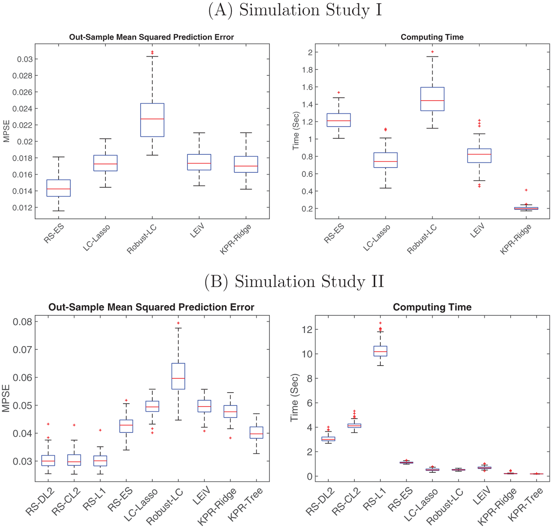
Boxplots of MPSE (left) and computing time (right) in (A) Simulation Study I and (B) Simulation Study II. This figure appears in color in the electronic version of this article, and any mention of color refers to that version

6.2 |. Study II: Tree-guided equi-sparsity setting

In this study, we include extrinsic information of a hierarchical tree. Data are generated in a similar way as in Study I, except for the true coefficients. To generate the coefficient vector, we first assume there is a tree structure among the variables (see Figure 3), where every 10 consecutive leaf nodes share a common parent node and so on. Guided by the tree structure, the true coefficient vector for the generative relative-shift model is set to be $\beta ={\left(1_{20}^T,-2\times 1_{10}^T,0.5\times 1_{10}^T,2\times 1_{40}^T,{\xi }_{20}^T\right)}^T$, where 1q is a length-_q vector of ones and ξ₂₀ is a length-20 vector filled standard Gaussian random numbers. Namely, in principle, the first 20 features can be aggregated along the tree to their common ancestor, the next 10 features can be aggregated to their parent node, and so on. The last 20 features, although they also share a common ancestor, cannot be aggregated due to distinct coefficient values. See Figure 3 for the feature aggregation pattern.

FIGURE 3.

Left: The taxonomic tree structure among variables in Study II. The leaf node indices are in ascending order from left to right. Right: The equi-sparsity structure of the regression coefficients. Features with the same coefficient are aggregated to the common ancestor (i.e., the closest solid node)

We compare the three tree-guided regularization methods RS-L1, RS-CL2, and RS-DL2 with all the competing methods. Among the competitors, only KPR-Tree takes advantage of the tree structure by converting it into a patristic distance kernel. The comparison result is shown in Figure 2B. In the left panel, the three tree-guided relative-shift methods have similar prediction errors and are significantly better than all the other methods. (More comparisons between the three proposed regularization methods can be found in Section A of Supporting Information.) The next best method is KPR-Tree, which benefits from the extrinsic tree structure. Among the methods not using the tree information, RS-ES outperforms the others. On the other hand, the superior prediction performance of the tree-guided relative-shift methods does come at a price, that is, a slightly higher computational cost. However, even with cross-validation for tuning parameter selection, the computing time of the proposed methods is within a few seconds for each simulation run (except for RS-L1). We also conduct additional simulations in higher-dimensional settings (for p = 400 and p = 1000). The proposed methods are quite scalable and the prediction results are similar to what we present here. More details can be found in Section A of Supporting Information.

7 |. APPLICATION TO PRETERM INFANT GUT MICROBIOME STUDY

We apply the proposed relative-shift model with taxonomic-tree-guided regularization to a preterm infant gut microbiome study. The study aims to understand how gut microbiome is related to the neurodevelopment of preterm infants. Data were collected at a Neonatal Intensive Care Unit (NICU) in the northeast US. Fecal samples of preterm infants were collected daily when available during the infant’s first month of postnatal age. Bacterial DNA was isolated and extracted from each sample; V4 regions of the 16S rRNA gene were sequenced using the Illumina platform. Gender, birth weight, delivery type, and complications were recorded at birth, and medical procedures and feeding types were recorded throughout the infant’s stay. Infant neurobehavioral outcomes were measured when the infant reached 36–38 weeks of post-menstrual age, using the NICU Network Neurobehavioral Scale (NNNS) (Cong et al., 2017; Sun et al., 2020).

After proper processing, we obtain p = 62 taxa, most at the genus level, on n = 34 individuals. The longitudinal data are averaged across the postnatal period for each infant, resulting in a single 34 × 62 OTU data matrix with 39.2% zero entries. Moreover, the taxonomic tree of the 62 taxa is also available (see Figure 4). Each taxon in the OTU table corresponds to a leaf node. The primary outcome is the normalized NNNS score. We also include several standardized covariates (i.e., gender, delivery type, premature rupture of membranes, score for Neonatal Acute Physiology–Perinatal Extension-II (SNAPPE-II), birth weight, and percentage of feeding with mother’s breast milk) in our analysis.

FIGURE 4.

The taxonomic tree of the NICU microbiome data. Taxa with the same estimated coefficient value (i.e., blank leaf nodes) are aggregated to their common ancestor (i.e., the closest solid node). The coefficient value (multiplied by 100) for each taxon (or group of taxa) is presented in the parenthesis. This figure appears in color in the electronic version of this article, and any mention of color refers to that version

Since all three tree-guided methods lead to similar results, we only present the result from RS-DL2 here. The tuning parameter is chosen by fivefold cross-validation. The estimated coefficients for compositional predictors are approximately equi-sparse but not exact. This is a common issue with the group-lasso-type penalty (Chen et al., 2012). To facilitate interpretation, we set a small threshold (i.e., 10⁻⁴) and truncate the groups of intermediate coefficients whose Frobenius norms are below the threshold. As a result, we obtain highly interpretable equi-sparse coefficients for the 62 taxa. An illustration of the estimated coefficient values and the corresponding feature aggregation pattern along the taxonomic tree is provided in Figure 4. In particular, taxa with the same coefficient are aggregated to the common ancestor (i.e., the lowest solid node). For instance, Taxa 2–6 at the genus level are aggregated to the common class Actinobacteria because they have the same estimated coefficient value.

The estimated coefficients carry intuitive interpretations of the microbial effects on the outcome. More specifically, the average value of $\widehat{\beta }$ (multiplied by 100) is 0.075, which provides an overall baseline for interpreting the parameters. Out of all the taxa, the Class Bacilli ($100\times {\widehat{\beta }}_j=0.317$ for j = 11, …, 23) and the Order Clostridiales ($100\times {\widehat{\beta }}_j=0.341$ for j = 24, …, 38) have the largest coefficient values, and the individual genera in the Order Enterobacteriales ($100\times {\widehat{\beta }}_j\le -0.228$ for j = 48, …, 56) have the smallest values. This indicates the outcome is (on average) positively associated with the composition of Bacilli and Clostridiales and negatively associated with the individual genera in Enterobacteriales. Moreover, if we shift one unit of concentration (i.e., 1% in proportion) from the Genus Shigella (a genus in Enterobacteriales) to any taxon (or taxa) in Clostridiales, the response value will increase by {3.41 − (−2.74)} × 10⁻³ = 6.15 × 10⁻³. Alternatively, if we move one unit of concentration from any taxon (or taxa) in Bacilli to any taxon (or taxa) in Clostridiales, the response value will only slightly increase by (3.41 − 3.17) × 10⁻³ = 2.4 × 10⁻⁴. Similarly, one could interpret the effect of shifting concentration between any two (groups of) taxa.

For comparison and corroboration, we also apply LC-Lasso with feature selection on the same data set. With the tuning parameter selected by cross-validation, the LC-Lasso method only selects three individual taxa at the genus level (i.e., Veillonella in Order Clostridiales, and Shigella and others in Order Enterobacteriales) after covariate adjustment. The directions of association are consistent with our findings (i.e., the genus in Clostridiales has positive association and the genera in Enterobacteriales have negative association). Although further investigations are warranted to validate the findings, the proposed method potentially provides a more comprehensive picture of the microbial effects on the outcome.

We further conduct leave-one-out cross-validation (LOOCV) to compare the out-sample prediction accuracy of different methods on the real data. The prediction squared errors (PSE) are summarized in Table 1. Due to the small sample size (n = 34), the differences between the methods are not statistically significant. The PSE are comparable between the relative-shift methods (RS-DL2 and RS-ES) and the log-contrast methods (LC-Lasso, KPR-Ridge, and KPR-Tree). Nonetheless, the intriguing biological interpretation of the proposed methods still warrants their use in this application. The estimated parameters may provide novel insights into the association between the gut microbiome and the neurodevelopmental outcome of preterm infants.

TABLE 1.

The median (median absolute deviation) of PSE of different methods based on LOOCV of the NICU data

Method	RS-DL2	RS-ES	LC-Lasso	KPR-Ridge	KPR-Tree
PSE	0.579 (0.484)	0.547 (0.448)	0.587 (0.509)	0.571 (0.493)	0.522 (0.475)

8 |. DISCUSSION

In this paper, we develop a novel relative-shift regression paradigm for compositional data. The new framework regresses the response on compositional predictors directly without transformation. The relative relation of coefficients for compositional predictors carry a straightforward interpretation, that is, the contrasts of coefficients capture effects of shifting concentration between features on the response. The relative-shift framework provides a flexible basis for supervised dimension reduction. We develop different regularization methods, that is, the equi-sparsity regularization and the tree-guided regularization, for feature aggregation. In particular, the tree-guided regularization takes advantage of the extrinsic hierarchical structure among features and adaptively identifies relevant features at different hierarchical levels. An efficient smoothing proximal gradient algorithm is devised to fit models with different regularization terms. Numerical studies demonstrate that the proposed methods provide an effective and interpretable alternative for compositional data analysis.

There are several directions for future research. First, in practice the effect of concentration shifts between parts of a composition on the response may be nonlinear, so it is of particular interest to generalize the current framework to accommodate such nonlinear relationships. Second, while we have established statistical guarantees on the prediction performance of the proposed method, it is pressing to study the estimation performance and develop statistical inference methods for assessing the relative-shift effects. To achieve these, certain comparability condition on the design is necessary (Bühlmann and van de Geer, 2009). Since the equi-sparsity pattern and the tree-structure are encoded in A where β* = Aγ*, such a condition could be imposed on the transformed design matrix XA.

Last but not least, although the current framework can handle zeros without replacement, it does not treat zero differently from any positive proportions. In many applications, it may be desirable to specifically model the zero generation mechanism (Xu et al., 2021).

DATA AVAILABILITY STATEMENT

The data that support the findings in this paper are provided by Dr. Xiaomei Cong. Restrictions apply to the availability of these data, which were used under license for this study. Data are available at https://figshare.com/s/8f0d7f9a5078c2030c2a with the permission of Dr. Xiaomei Cong (xiaomei.cong@uconn.edu).

REFERENCES

- Aitchison J (1982) The statistical analysis of compositional data. Journal of the Royal Statistical Society: Series B, 44,139–160. [Google Scholar]
- Aitchison J (1983) Principal component analysis of compositional data. Biometrika, 70, 57–65. [Google Scholar]
- Aitchison J & Bacon-Shone J (1984) Log contrast models for experiments with mixtures. Biometrika, 71, 323–330. [Google Scholar]
- Aitchison J & Egozcue JJ (2005) Compositional data analysis: where are we and where should we be heading? Mathematical Geology, 37, 829–850. [Google Scholar]
- Beck A & Teboulle M (2009) A fast iterative shrinkage-thresholding algorithm for linear inverse problems. SIAM Journal on Imaging Sciences, 2,183–202. [Google Scholar]
- Bien J, Yan X, Simpson L & Muller CL (2020) Tree-aggregated predictive modeling of microbiome data. bioRxiv. [DOI] [PMC free article] [PubMed] [Google Scholar]
- Bien J, Yan X, Simpson L & Muller CL (2021) Tree-aggregated predictive modeling of microbiome data. Scientific Reports, 11(1), 1–13. [DOI] [PMC free article] [PubMed] [Google Scholar]
- Bühlmann P & van de Geer S (2009) Statistics for High-Dimensional Data. Berlin: Springer. [Google Scholar]
- Chen X, Lin Q, Kim S, Carbonell JG & Xing EP (2012) Smoothing proximal gradient method for general structured sparse regression. The Annals of Applied Statistics, 6, 719–752. [Google Scholar]
- Combettes PL & Muller CL (2021) Regression models for compositional data: General log-contrast formulations, proximal optimization, and microbiome data applications. Statistics in Biosciences, 13, 217–242. [Google Scholar]
- Cong X, Judge M, Xu W, Diallo A, Janton S, Brownell EA et al. (2017) Influence of infant feeding type on gut microbiome development in hospitalized preterm infants. Nursing Research, 66, 123–133. [DOI] [PMC free article] [PubMed] [Google Scholar]
- Garcia TP, Muller S, Carroll RJ & Walzem RL (2013) Identification of important regressor groups, subgroups and individuals via regularization methods: application to gut microbiome data. Bioinformatics, 30, 831–837. [DOI] [PMC free article] [PubMed] [Google Scholar]
- Gloor GB, Wu JR, Pawlowsky-Glahn V & Egozcue JJ (2016) It’s all relative: analyzing microbiome data as compositions. Annals of Epidemiology, 26, 322–329. [DOI] [PubMed] [Google Scholar]
- Greenacre M (2020) Amalgamations are valid in compositional data analysis, can be used in agglomerative clustering, and their log-ratios have an inverse transformation. Applied Computing and Geosciences, 5, 100017. [Google Scholar]
- Hastie T, Tibshirani R & Wainwright M (2019) Statistical Learning with Sparsity: The Lasso and Generalizations. London: Chapman and Hall/CRC. [Google Scholar]
- Kim S, Sohn K-A & Xing EP (2009) A multivariate regression approach to association analysis of a quantitative trait network. Bioinformatics, 25, i204–i212. [DOI] [PMC free article] [PubMed] [Google Scholar]
- Li H (2015) Microbiome, metagenomics, and high-dimensional compositional data analysis. Annual Review of Statistics and Its Application, 2, 73–94. [Google Scholar]
- Lin W, Shi P, Feng R & Li H (2014) Variable selection in regression with compositional covariates. Biometrika, 101,785–797. [Google Scholar]
- Nesterov Y (2005) Smooth minimization of non-smooth functions. Mathematical Programming, 103,127–152. [Google Scholar]
- Palarea-Albaladejo J & Martin-Fernandez J (2013) Values below detection limit in compositional chemical data. Analytica Chimica Acta, 764, 32–43. [DOI] [PubMed] [Google Scholar]
- Randolph TW, Zhao S, Copeland W, Hullar M & Shojaie A (2018) Kernel-penalized regression for analysis of microbiome data. The Annals of Applied Statistics, 12, 540–566. [DOI] [PMC free article] [PubMed] [Google Scholar]
- She Y (2010) Sparse regression with exact clustering. Electronic Journal of Statistics, 4,1055–1096. [Google Scholar]
- Shi P, Zhang A & Li H (2016) Regression analysis for microbiome compositional data. The Annals of Applied Statistics, 10, 1019–1040. [Google Scholar]
- Shi P, Zhou Y & Zhang A (2021) High-dimensional log-error-in-variable regression with applications to microbial compositional data analysis. Biometrika, 109, 405–420. [Google Scholar]
- Silverman JD, Washburne AD, Mukherjee S & David LA (2017) A phylogenetic transform enhances analysis of compositional microbiota data. Elife, 6, e21887. [DOI] [PMC free article] [PubMed] [Google Scholar]
- Sun Z, Xu W, Cong X, Li G & Chen K (2020) Log-contrast regression with functional compositional predictors: linking preterm infant’s gut microbiome trajectories in early postnatal period to neurobehavioral outcome. The Annals of Applied Statistics, 14, 1535–1556. [DOI] [PMC free article] [PubMed] [Google Scholar]
- Tsilimigras MC & Fodor AA (2016) Compositional data analysis of the microbiome: fundamentals, tools, and challenges. Annals of Epidemiology, 26, 330–335. [DOI] [PubMed] [Google Scholar]
- Wang T & Zhao H (2017) Structured subcomposition selection in regression and its application to microbiome data analysis. The Annals ofApplied Statistics, 11, 771–791. [Google Scholar]
- Xia Y, Sun J & Chen D-G (2018) Statistical analysis of microbiome data with R (Vol. 847) Singapore: Springer. [Google Scholar]
- Xu T, Demmer RT & Li G (2021) Zero-inflated poisson factor model with application to microbiome read counts. Biometrics, 77, 91–101. [DOI] [PMC free article] [PubMed] [Google Scholar]
- Yan X & Bien J (2021) Rare feature selection in high dimensions. Journal of the American Statistical Association, 116, 887–900. [Google Scholar]
Associated Data
This section collects any data citations, data availability statements, or supplementary materials included in this article.
Supplementary Materials