The impacts of spatial resolutions on global urban-related change analyses and modeling

Summary

Various global land use/land cover (LULC) products have been developed to drive land-relevant climate and hydrological models for environmental assessments. However, systematic studies remain scarce that assess the uncertainties of using these products. By using a total of 16 commonly used global LULC products, we find a logarithm law of upscaling with the spatial resolution. The law reveals spatial details of urban features will be majorly distorted when using LULC products with coarser resolutions. A tipping point of the law around the 30-m resolution was identified by additional analysis of the 1-m and 10-m local land use dataset. Through the example of assessing crop production loss, we further find that most of these products will yield a significant underestimation of crop production losses, globally and locally. We conclude that the underestimated urban land rooted in most of these products would cause vital impacts on global change analyses and modeling.

Graphical abstract

Highlights

• •A logarithm law can portray the underestimation of urban land by LULC products
• •A potential tipping point of the law is found at around the 30-m resolution
• •Urban features will be majorly distorted when using coarsening products
• •Coarse resolutions yield a significant underestimation of crop production losses

Earth sciences; Earth-surface processes; Agricultural science; Land use.

Introduction

For the last three decades, large-scale land cover changes have occurred to the Earth, driven by the force of economic development and population growth.¹ Land use/land cover (LULC) change, such as urban encroachment, farmland reclamation, and deforestation, have significant consequences on ecological and biogeochemical cycles,^2,3 biodiversity,⁴ hydrological processes,⁵ and the carbon fluxes of terrestrial ecosystems.^6,7 Such impact will not abate as the urban population and urban land will continue until 2050.⁸

LULC products, usually created by remote sensing, provide rich and critical temporal information for recording the important dimensions of global changes on earth surfaces. Producing time-series of land cover data can satisfy the needs of modeling communities which want to understand and predict the processes of the Earth systems.⁹ Most of these studies require the description of the properties of earth surfaces in terms of albedo, roughness, evapotranspiration, surface fluxes, and carbon storage. These factors are difficult to acquire at the global scale, but can be quantified or modeled by mainly using the information of land use types.¹⁰ Besides the climate, hydrological and ecological modeling, LULC maps are important for tackling various resource management issues in terms of the conservation of farmlands, forests and biodiversity, and prevention of watershed degradation and desertification. These maps thus provide valuable information for governments and organizations to formulate climate change mitigation and adaptation policies.^11,12

Accurate and updated land cover information will assure the better performance of geographical analysis and environmental modeling, and facilitate the understanding of geographical processes.^13,14,15 However, it is extremely difficult to obtain LULC maps at the global scale because the classification involves large data volumes and labor-intensive jobs. In the 1980s, land cover maps, especially at the global scale, were only produced at the spatial resolutions ranging from 1° to 0.5°, for addressing the needs of climate modeling and carbon cycling studies, etc.^16,17 Special treatment is required to deal with such coarse resolution because of mixed land use types within a large pixel. A practical way to obtain global land cover with such a large pixel size (e.g., 0.5 × 0.5 degree) is to represent the land use by using the dominant land use type.^18,19 For example, fractional land use types (e.g., crop, pasture, and urban) at a resolution of 0.5 × 0.5 degree were obtained as a common base for climate modeling.²⁰ A later effort was to develop the method that addresses land management explicitly as a component of land systems at a spatial resolution of 5 arcminute (i.e., 9.25 × 9.25 km)¹⁴ Such resolution only represents the land cover by a mixture of different land use types for each individual grid cell. However, many other applications, such as those related to agriculture, resource management, environmental assessment and urban planning, have to rely on much finer resolutions, because of the heterogeneity of land use patterns.^21,22 The demand also comes from a new generation of process models which try to capture the dynamic of the Earth systems more accurately.²³

In the recent three decades, the growing demand for high-resolution land use information has resulted in marvelous progress in producing various global LULC products. The endeavor has enabled global land cover/use data available at various spatial resolutions, such as 1 km GlobCover (Global Land Cover),^9,24,25 500 m MODIS (Moderate Resolution Imaging Spectroradiometer),^26,27 300 m GlobCover,²⁸ and 30 m FROM-GLC (Finer Resolution Observation and Monitoring of Global Land Cover) and GlobeLand30 (30 m Global Land Cover) products.^29,30 Higher spatial resolutions are usually at the cost of lower temporal resolutions because of the difficulty in producing these products globally. For example, GlobeLand30 is only available for the years 2000 and 2010 so far.³⁰

Most of the applications may face the dilemma of choosing a LULC product with either finer spatial or finer temporal resolutions. The selection of a product may be determined by many issues, such as model requirements, data availability, and computation capability. In most situations, environmental assessments and modeling require the inputs of updated and detailed land cover information. Accurate area of land use types should be obtained as the primary input to the analysis and modeling practice. For example, the Integrated Valuation of Ecosystem Services and Trade-offs (InVEST) mainly relies on the input of detailed land use types to estimate the carbon storage.³¹ Studies have shown that spatial resolutions coarser than 1 km for land cover data will attribute to significant biases in the identification of urban features, and estimation of terrestrial carbon sequestration and its interannual variability.³² By using the maps with resolution coarser than 5 km, the analytical results may contain at least 5% area estimation error for most land use types.²¹ Instead, Chen et al.³⁰ indicated that the most significant human activities should be captured by the satellite data with a 30-m resolution.

The above analyses related to the use of these products were generally carried out at a regional scale, without a systematic study at the global scale. Geographical scale effect is a major issue encountered in geographical analyses and assessments.³³ Although various studies have been carried out to assess the accuracies of LULC products through rigorous validations according to some international standards,²⁸ the impact of spatial resolutions on change-related analysis and modeling has not been well examined in a systematic way at the global scale. Considering this, the objective of this paper is to assess the impact of product resolutions on mapping global urban land and related assessments (e.g., the estimation of crop production losses). We focus on the urban land change which plays a vital role in altering various ecological and hydrological processes. In the application, the immediate effect of land use change is the crop production losses because of urban encroachment on farmland.⁸ The crop production losses, either in the past and the future, should be an important issue because ensuring food security is of key importance to achieve the goal of Zero Hunger, which is one of 17 Sustainable Development Goals (SDGs) proposed by the United Nations.³⁴

To quantify the impacts of spatial resolution on the change-related analysis and assessments, we conducted the experiments in two ways. First, the Pearson correlation coefficient was adopted to examine the relationship between the spatial resolution and the global urban area. With the use of 16 sets of commonly used LULC products, there is a large span of spatial resolutions, ranging from 30 m to 50 km respectively. For the resolution below 30 m, the LULC products at the global scale are unavailable. We had to select ten cities in the US which have 1-m land use data, plus 10-m data classified by Tsinghua University’s LULC group, who is the author of the 30 m FROM-GLC product.^29,35 As there are many other sources of uncertainties, we then tried to spatially aggregated the same high-resolution maps by coarsening them (the 30-m GlobeLand30_ATS2010 product) to look at the pure relationships between the resolution and the urban area. Finally, we quantitatively estimated the crop production losses caused by historical and future urban expansion. The analysis will help understand the scaling effects of LULC products on geographical modeling and environmental assessments (e.g., crop production estimation).

Results

The logarithm law of estimating global urban area

Overall relationship

Figure 1 illustrates the effect of spatial resolution on mapping the urban details of the Pearl River Delta, China. It is apparent that a finer resolution product, like GHS-BUILT (38-m resolution), can map the urban land with much more spatial details, being close to the realistic patterns. As the spatial resolution decreases, the small patches of urban land disappear rapidly. We can only observe very a vague configuration of the land use patterns, e.g., in GLCNMO_V1 data (Figure 1C). The layout of cities becomes much distorted as small patches of urban land are almost wiped out in GAEZ-Dom of a 10-km resolution (Figure 1D).

Figure 1.

Layout of urban land in the Pearl River Delta, China, using different spatial resolution products

(A) GHS-BUILT, 38 m, 2014. (B) MODIS/MCD12Q1, 500 m, 2010. (C and D) GLCNMO_V1, 1 km, 2003; and (d) GAEZ-Dom, 10 km, 2010.

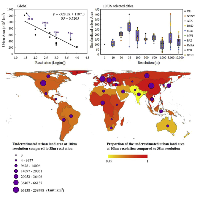
With the use of a total of 16 global LULC products, we retrieved the global urban land to explore the scaling effect on estimating urban land (Table 1 and Figure 2). Figure 3 shows there exists a quite strong linear relationship in a logarithm form between the data resolution and the amount of global urban land. The overall Pearson correlation coefficient is as high as −0.831, with a significance level of 0.01. The value of R² is 0.72, indicating a good level of explanation. This analysis reveals that a coarser resolution will result in a severe underestimation of global urban land for these commonly used products. In other words, we can obtain more urban details by using a finer resolution product to capture global urban land. The underestimation of global urban area is 63%, if the resolution decreases from 500 m ($\log \left(m\right)=2.70$) to 10 km ($\log \left(m\right)=4$). The underestimation becomes as high as 83%, whereas dropping from 30 m ($\log \left(m\right)=1.48$) to 10 km. If the spatial resolution is 1 m ($\log \left(m\right)=0$), we may even infer that the global urban area would be 1.51 million km² (i.e., the slope value) for the year 2010, which is 24% higher than that estimated by using the 30-m LULC product. The estimation of the global urban area at 1-m resolution has not been carried out before as the job is much data demanding and labor intensive.

Table 1.

A total of 16 global land cover datasets with the spatial resolutions ranging from 30 m to 50 km

Global land cover data	Abbreviation	Resolution	Year	Landtype name	Data source
30 m Global Land Cover data product	GlobeLand30_ATS2010	30 m	2010	Artificial surfaces	http://www.geodoi.ac.cn/WebCn/doi.aspx?Id=163
Global Human Settlement Layer: Built-up	GHS-BUILT	38 m	2014	Built-up areas	http://data.jrc.ec.europa.eu/collection/ghsl
European Space Agency, Climate Change Initiative Climate Research Data Package	ESA-CCI	300 m (10″)	2010	Urban areas	http://maps.elie.ucl.ac.be/CCI/viewer/download.php
Global Land Cover Map	GlobCover	300 m (10″)	2009	Artificial surfaces and associated areas (urban areas >50%)	http://dup.esrin.esa.it/page_globcover.php
MODIS Land CoverType product	MODIS/MCD12Q1	500 m (15″)	2010	Urban and built-up land	https://lpdaac.usgs.gov/dataset_discovery/modis/modis_products_table
Global Land Cover by National Mapping Organizations Version 3	GLCNMO_V3	500 m (15″)	2013	Urban	https://globalmaps.github.io/
Spatial Distribution and Density of Constructed Impervious Surface Area	ISA	1 km (30″)	2010	Impervious surfaces	https://www.ngdc.noaa.gov/eog/dmsp/download_global_isa.html
Global Land Cover-SHARE	GLC-SHARE	1 km (30″)	2014	Artificial surfaces	http://www.glcn.org/databases/lc_glcshare_en.jsp
Global Land Cover 2000 database	GLC2000	1 km (30″)	2000	Artificial surfaces and associated areas	http://forobs.jrc.ec.europa.eu/products/glc2000/glc2000.php
Global Land Cover by National Mapping Organizations Version 1	GLCNMO_V1	1 km (30″)	2003	Urban	https://globalmaps.github.io/
Global Land System classification data	GLS	9,250 m (5′)	2010	Urban, peri-urban and villages	http://www.environmentalgeography.nl/site/data-models/data/global-land-system-classification/
Global Agro-ecological Zones-Dominant Land Cover and Use	GAEZ-Dom	10 km (5′)	2007	>50% Build-up land	http://www.fao.org/geonetwork/srv/en/metadata.show?id=38215&currTab=simple
Food Insecurity, Poverty and Environment Global GIS Database	FGGD	10 km (5′)	2007	>50% Artificial surfaces	http://www.fao.org/geonetwork/srv/en/metadata.show?id=14071&currTab=simple
Global Historical Land-Cover Change and Land-Use Conversions-HH	ISAM-HH (Integrated Science Assessment Model)	50 km (0.5°)	2005	Urban land	https://www.atmos.illinois.edu/∼meiyapp2/datasets.htm
Global Historical Land-Cover Change and Land-Use Conversions-HYDE (Historical Database of the Global Environment)	ISAM-HYDE (Integrated Science Assessment Model)	50 km (0.5°)	2010	Urban land	https://www.atmos.illinois.edu/∼meiyapp2/datasets.htm
Global Historical Land-Cover Change and Land-Use Conversions-RF	ISAM-RF (Integrated Science Assessment Model)	50 km (0.5°)	2007	Urban land	https://www.atmos.illinois.edu/∼meiyapp2/datasets.htm

Figure 2.

Visual inspection of GlobCover data (300-m resolution) and GLCNMO_v1 data (1-km resolution) for urban land cover (red grids)

(A) GlobCover, 300m, 2009; (B) GLCNMO_V1, 1km, 2003; (C and D) are the stepwise zoom-in of (A) respectively.

Figure 3.

The logarithm law depicting the relationship between the data resolution and the global urban area by using a total of 16 LULC products

In contrast to Figure 3, Figure 4 shows the change in global urban area when aggregating the 30-m resolution product to coarser its original resolution. Not surprisingly, the results obtained by this coarsening approach still show strong linear relationship in a logarithm form between the data resolution and the amount of global urban land. The R² value is as high as 0.89, which is higher than the R² value (0.72) obtained from the use of the 16 LULC products. The improvement of the R² value is due to the use of a single dataset. In other words, the uncertainties brought by different products can be explained by the decrease of the R².

Figure 4.

The logarithm law depicting the relationship between the data resolution and the global urban area by aggregating the 30-m GlobeLand30_ATS2010 product

The underestimation of global urban area by aggregating the maps from 500 m ($\log \left(m\right)=2.70$) to 10 km ($\log \left(m\right)=4$) is 64%, whereas the underestimation from 30 m ($\log \left(m\right)=1.48$) to 10 km is 68%. This result has demonstrated that the strong linear relationship in a logarithm form between global urban area and data resolution still exists under this aggregation approach. As a comparison, the actual underestimated urban land area at 10-km product (i.e., GAEZ-Dom) across the globe reaches to 1,061,191 km² (approximately 83.61% of the global urban land area at 38-m resolution) based on the 38-m product (GHS-BUILT). Figure 5 shows the actual amount and proportion of underestimated urban land area at 10km resolution compared to the 38 resolution by region.

Figure 5.

The underestimated urban land area in different regions across the world at 10-km product (GAEZ-Dom) compared with 38-m product (GHS-BUILT)

The logarithm laws by regions

There is significant geographical heterogeneity across the world in terms of climate and ecosystem characteristics. Therefore, we established the individual logarithm laws by 26 world regions which are defined via referring to Stehfest et al.³⁶ This yielded the individual relationship between the data resolution and the urban land area, presenting the individual Pearson correlation coefficients for each region. Table 2 shows that all these regions have a negative coefficient corresponding to the data resolution. This means that a coarse resolution will unanimously cause the decrease in urban area. According to Table 2 and Figure 6, the correlation coefficients of 17 geographical regions are at a significance level of 0.01. Their coefficient values are very high, ranging from −0.656 in Japan to −0.861 in Canada. Almost all these regions are on the continents of Europe, Asia and North America. Most human activities exist in these regions, which also share a large portion of the world population. There are six regions with a significance level of 0.05, including Central Asia, Korea region, Western Africa, Indonesia region, Northern Africa, and the Rest of Southern Africa (all of them are in the continents of Africa and Asia). Only the regions in the Rest of South America, Oceania and Brazil have not shown a significant association between the data resolution and urban area, despite their correlation coefficients are negative, implying a similar trend compared to other regions.

Table 2.

The Pearson correlation coefficients between data resolution and urban area in different world regions

Regions	Central Europe	Rest of South America	Oceania	Brazil	Canada
Coefficients	−0.777∗∗	−0.439	−0.409	−0.441	−0.861∗∗
Regions	China region	Central America	Russia region	Western Europe	Northern Africa
Coefficients	−0.851∗∗	−0.748∗∗	−0.727∗∗	−0.764∗∗	−0.595∗
Regions	Eastern Africa	Western Africa	Indonesia region	India	Middle East
Coefficients	−0.669∗∗	−0.54∗	−0.567∗	−0.734∗∗	−0.706∗∗
Regions	Japan	Central Asia	Korea region	Mexico	Rest of Southern Africa
Coefficients	−0.656∗∗	−0.568∗	−0.611∗	−0.694∗∗	−0.591∗
Regions	Rest of South Asia	Turkey	Ukraine region	The United States	South Africa
Coefficients	−0.677∗∗	−0.698∗∗	−0.684∗∗	−0.695∗∗	−0.733∗∗
Regions	Southeast Asia
Coefficients	−0.738∗∗

Significance levels: ∗∗p = 0.01; ∗p = 0.05.

Figure 6.

The global map of the Pearson correlation coefficients between spatial resolution and urban area estimation for 26 world regions

The above analysis reveals that the variant of the logarithm law corresponding to the spatial heterogeneity of urban configuration across the globe. If the urban distribution is more clustered and contiguous (Figure 7A), there is less degree of underestimating urban area. In contrast, the urban area estimation is more sensitive to the choice of the land-cover product resolutions if the urban land distribution in a region is more discrete and dispersed (Figure 7B). This can be better understood by using an extreme scenario (e.g., all non-urban land has been converted into urban land). In this situation, choosing different spatial resolutions to map the urban land will cause no or very limited bias. The great area-estimation bias caused by coarse spatial resolutions reflects the uneven distribution of global urban land, i.e., most of human activities dispersed by occupying very small patches of land on the Earth’s surface.

Figure 7.

Urban land with a more contiguous distribution (A) and with a more dispersed distribution (B)

Verification at 1-m and 10-m resolution using selected cities in the US

The 30-m resolution is the most commonly used and relatively high resolution for LULC products at a global scale so far. It should be attractive to verify the logarithm law beyond this limit by using higher spatial resolutions (e.g., 1-m and 10-m resolution). As the global LULC products with such high resolution do not exist, we have to select some cities in the US which have the land use map of 1-m resolution for the verification. Table 3 lists the input data sources from EnviroAtlas (https://www.epa.gov/enviroatlas) for ten selected cities in the US. For the urban map of 10-m resolution for these cities, the data were prepared by Tsinghua University’s LULC group, who is the author of the 30 m FROM-GLC product.^29,35

Table 3.

Input data sources of the ten selected cities with the 1-m resolution products from the EnviroAtlas

City	Abbreviation	Input data source	Year
New York in New York	NYNY	Aerial photography	2011
		LiDAR data	2010
Chicago in Illinois	CIL	Aerial photography	2010, 2012, 2013
		LiDAR data	2006, 2007, 2008, 2010, 2013, 2014
Austin in Texas	ATX	Aerial photography	2010
		LiDAR data	2007
Baltimore in Maryland	BMD	Aerial photography	2013
		LiDAR data	2011, 2015
Memphis in Tennessee	MTN	Aerial photography	2012, 2013
		LiDAR data	2009–2012
Milwaukee in Wisconsin	MWI	Aerial photography	2010
		LiDAR data	2010, 2012
Philadelphia in Pennsylvania	PhiPA	Aerial photography	2013
		LiDAR data	2006–2008, 2011–2015
Phoenix in Arizona	PAZ	Aerial photography	2010
Portland in Oregon	POR	Aerial photography	2011, 2012
		LiDAR data	2007, 2010
Washington, District of Columbia	WDC	Aerial photography	2013, 2014
		LiDAR data	2002–2016

At first, we estimated the urban areas of New York and Chicago to get some insights on the scaling effects using the LULC data ranging from 1-m to 50-km resolutions. The 1-m resolution maps show that the impervious areas in New York and Chicago account for 44 and 15% of the total land areas, respectively. Figures 8 and 9 show the estimated urban areas of New York and Chicago from these data. When the resolution is in the range from 1 m to 1 km, the estimated urban areas increase as the resolution becomes finer, in line with the overall relationship globally. The urban areas will reach a peak value, and then drop as the resolution becomes finer. Specifically, the urban areas reach their maximum if the resolution is in the range of 10–40 m for both these two cities. When the resolution is larger than 1 km, the urban areas of the two cities only have some subtle changes without an obvious decreasing trend. It is because that New York and Chicago are two megacities, having large amounts of contiguous urban parcels. In the practice of land classification in remote sensing, as we know, the land type of a cell is assigned with the dominant land type within the cell. Thus, urban land still prevails even if the resolution is 10 km in the extent of these two cities. This explains why the estimated urban areas of New York and Chicago have not decreased significantly between the resolutions of 1 km and 10 km. In addition, the urban land accounts for 44% of the total land in New York. The percentage is near 60%, if we exclude the water body within New York’s administrative boundary. Because of the high proportion of urban land, New York has a higher possibility to identify more urban cells when the resolution becomes coarser, showing a different estimation trend regarding to the law.

Figure 8.

Urban area of New York in data sources of different resolutions

Figure 9.

Urban area of Chicago in data sources of different resolutions

Figures 10 and 11 show the urban land patterns of New York and Chicago by different resolutions, respectively. For New York, the change of resolution from 38 m to 10 km (Figures 10D–9G) has not significantly affected the area size of urban land. Chicago, which has a lower percentage of urban land, has a significant decrease in urban area when the resolution decreases from 38 m to 10 km (Figures 11D–10G). By zooming in the core areas of these two cities (Figures 10A–9C for New York and Figures 11A–10C for Chicago), we found that the identified urban area decreases as the resolution increases from 30 m to 1 m. This is mainly because the urban area, under the coarse resolution, would be merged into its background, namely, the non-urban area. This indicates that other land use types surrounding by urban pixels are possible to be merged into urban areas when aggregating the 1-m resolution product to coarser resolution data. For instance, the forest pixels surrounding by urban area in Figure 10A has been identified to be forest rather than “urban land” at a very fine scale. Despite a product with a finer resolution may not always identify a larger urban area, a fine-scale product helps us better delineate the urban morphology, for its capability of capturing much more land details.

Figure 10.

Urban land patterns of New York at different resolutions

(A) 1 m from EnviroAtlas; (B) 10 m from Tsinghua University; (C) 30 m from GlobeLand30_ATS2010; (D) 38 m from GHS-BUILT; (E) 300 m from ESA-CCI; (F) 1 km from GLCNMO_V3; (G) 10 km from GAEZ-Dom.

Figure 11.

Urban land patterns of Chicago at different resolutions

(A) 1 m from EnviroAtlas. (B) 10 m from Tsinghua University. (C) 30 m from GlobeLand30_ATS2010. (D) 38 m from GHS-BUILT. (E) 300 m from ESA-CCI. (F) 1 km from GLCNMO_V3. (G) 10 km from GAEZ-Dom.

We further selected more cities in the US to examine the relationship or the law, by including 1-m and 10-m resolutions. A total of ten cities were selected, including Austin (ATX), Baltimore (BMD), Chicago (CIL), Memphis (MTN), Milwaukee (MWI), New York (NYNY), Phoenix (PAZ), Philadelphia (PhiPA), Portland (POR), and Washington (WDC). For each of these cities, we calculated the urban area by using the LULC data ranging from 1 m to 50 km. To support the comparison, for each city, we treated the urban area estimated from 1-m resolution as the standard value (i.e., 100), the urban areas estimated from other resolutions are then standardized, divided by the urban area at 1-m resolution and multiplied by 100. By this standardization, we can compare their urban area distribution by using 180 sample points (18 datasets × 10 cities) (Figure 12), and generalize the aggregated urban area distribution by summing up the total area of 10 cities (Figure 13).

Figure 12.

Standardized urban area distribution of ten US selected cities in different resolution products

Figure 13.

Total urban area of ten US selected cities in different resolution products

Both Figures 12 and 13 show that the largest value of urban area can be observed when using the land cover product of a 38-m resolution, showing a tipping point for the logarithm law around this resolution. We thus conclude that 30 m (or 38 m) in general may be the most suitable spatial scale, for it has the possibility to capture the largest amount of urban area, without missing much information of urban land but with good data availability. If our research focuses on the issues that need to deal with at a very fine scale (i.e., below 30 m in this paper), it is necessary to rethink the definition of “urban land”, because at this scale, more urban details can be presented. For example, the green infrastructure within or surrounded by urban land (e.g., buildings and roads) can be delineated and separated from urban land.

Impacts on crop production estimation by resolution

The input of accurate land use information is essential for most of the climate and hydrological modeling and environmental assessments. We will examine how the spatial resolution of these LULC products will affect the accurate estimation of crop production losses associated with urban expansion. Table 4 shows that the global urban expansion in 2003–2013 was 187,494 km² and 175,308 km² respectively, by using the GLCNMO and ESA-CCI LULC products (shown in Table 5). These estimations are much higher than that of using the ISAM-HYDE product, by which we can only observe an increased urban area of 39,650 km² globally. Note that, the spatial resolution of the GLCNMO product is close to the ESA-CCI’s, but has changed from 1,000 m in 2003 to 500 m in 2013. The resolution increase may lead to more amounts of estimated urban expansion. As a result, we can observe a slightly higher increase of urban area from the GLCNMO product, compared with that from the ESA-CCI product.

Table 4.

Urban encroachment and crop production loss by using different LULC products

	LULC products
	ESA-CCI (2003–2013) (300-m resolution)	GLCNMO (2003–2013) (1-km resolution)	ISAM-HYDE (2000–2010) (50-km resolution)
Increased urban areas (km2)	187,494	175,308	39,650
Area increase rate (%)	36.44	50.46	12.25
Encroached cropland areas by urban expansion (km2)	116,597	131,120	18,909
Global production loss (billion kg)	51.86	60.16	5.21

Table 5.

List of empirical data used for estimating crop production losses

Data	Abbreviation	Year	Resolution	Data source
Spatial Production Allocation Model	SPAM	2010	10 km (5′)	https://www.mapspam.info/
European Space Agency, Climate Change Initiative	ESA-CCI	2003 2013	300 m (10″)	http://maps.elie.ucl.ac.be/CCI/viewer/download.php
Global Land Cover by National Mapping Organizations	GLCNMO_V1, GLCNMO_V3	2003 2013	1 km (V1), 500 m (V3)	https://globalmaps.github.io/
Global Historical Land-Cover Change and Land-Use Conversions-HYDE (Historical Database of the Global Environment)	ISAM-HYDE	2000, 2010	50 km (0.5°)	https://www.atmos.illinois.edu/∼meiyapp2/datasets.htm

As shown in Table 4, we observed the highest production loss (60.16 billion kg) using the GLCNMO product, followed by the loss (51.86 billion kg) using the ESA-CCI product. These two products have similar spatial resolutions, resulting in a similar level of crop production loss. Because the ISAM-HYDE’s spatial resolution is much coarser, we only observed a much less amount of urban expansion and crop production loss (5.21 billion kg). We can find that the yield from the ISAM-HYDE is significantly underestimated, which is only a tenth of that from the ESA-CCI product.

Based on the SPAM data, we obtained that in 2010, the global crop production of rice, wheat, maize, potato, and vegetables were 702.98, 674.75, 853.15, 346.37, and 918.59 billion kg respectively. Encroached by global urban expansion, vegetable faced the largest amounts of production loss, ranging from 28.79 billion kg (GLCNMO), 22.52 billion kg (ESA-CCI) to 1.53 billion kg (ISAM-HYDE) (corresponding data are shown in Table 5). In contrast, potato had the smallest amounts of production loss, ranging from 3.48 to 0.50 billion kg. Specifically, the crop production losses varied among different world regions because of the spatial heterogeneity. Figure 14 shows the rice production loss and cropland loss due to urban expansion, whereas other crop production loss (e.g., wheat, maize, potato, and vegetable) because of urban expansion are shown in Figures S1–S4. China faced a very high level of production loss for all the crop types, mainly because of its rapid urbanization in recent decades. Particularly, China was the only country having a significant decline in vegetable production, accounting for 72.55% of the total loss in the world. This could be a severe issue for sustainable urban development that needs to address the food security issue immediately. Surprisingly, Indonesia and Southeast Asia, which are the main rice production regions in the world, faced a high decline in the rice production. High loss in the potato production and wheat production also took place in Western Europe. India had a high loss in the potato production, followed by rice production. In terms of the US, it only faced a relatively high level of loss in the maize production, which may be explained by the fact that the general process of rapid urban expansion had ended in this country for a long time.

Figure 14.

Rice production loss and cropland because of urban expansion for various geographical regions

(A) rice production loss. (B) cropland loss. Note: ESA-CCI, 300 m, 2003–2013; GLCNMO, 1 km (2003)/500 m (2013), 2003–2013; ISAM-HYDE, 50 km, 2000–2010.

We can observe similar impacts of spatial resolutions on crop production estimation for different crop types and in different regions. For almost every crop type and every region, the ESA-CCI or GLCNMO product helps us better capture the details of crop production loss, which are much higher compared to the loss estimated by using the ISAM-HYDE product. The estimation bias is greater in main production areas for some crop types, like the rice in China, the wheat in Western Europe and the potato in India.

The above analysis revealed the biases in estimating historical crop production losses because of urban expansion from various land cover products. A further step was to investigate the scaling effects on the modeling process by using a land-use simulation model. The future LULC maps with 1-km resolution under four development scenarios created by Li et al.³⁷ were used to estimate the potential crop production losses because of the future urban expansion (Figure 15). We assumed the crop production loss estimated at the 1-km resolution as the “true” production loss, because this resolution is the highest so far for future global LULC.⁸ Figure 16 shows the relationship between the true loss rate of production caused by urban expansion and the identification rate of the true production loss at different resolutions. In the X axis, the true loss rate of production is estimated from the ratio of true loss to total production, which reflects the severity of the true loss. In the Y axis, the identification rate of the true production loss is the ratio of the estimated production loss at a coarse resolution to the true loss, which reflects the degree or severity of the underestimation. Each color dot in the figure represents a crop type in a scenario. For example, rice has four color dots in each subgraph, corresponding to the four scenarios in the future LULC maps. The blue line in the upper part of the subgraphs indicates the case where 100% (perfect identification) of the lost production/area is identified. The different colored circles on the blue line represent where their corresponding points should be in the case of 100% perfect identification. It means that the farther these points are from the blue line, the lower (poorer estimation) the lost production/area identification rate. The linear regression equations in the three subgraphs demonstrate a significant correlation at different scales. The results show that the lower the true loss rate, the lower the identification rate of production loss, which reflects those coarse resolutions tend to miss small-scale production loss cases. Furthermore, using coarse-resolution products for production loss estimation can lead to greater underestimation where the true loss rate is the same (the intercept becomes smaller as the resolution is coarser).

Figure 15.

Distortion of urban features in the land use simulation under the A1B Scenario in selected metropolitan areas with various spatial resolutions (1-km, 10-km, 30-km and 50-km resolutions)

Figure 16.

Rate of true production loss and true cropland loss because of urbanization

True loss rate of production and true loss rate of cropland area are estimated at 1-km product. Rates of true production loss and cropland loss are calculated by losses at multiple resolution products and the 1-km product.

Discussion and conclusion

Only occupying a small portion of the global land, the urban areas that are characterized with intensive human activities have created major disturbance to the ecosystems. Even a small percentage increase in the urban areas can significantly alter climate, biogeochemistry, and hydrology at local, regional, and global scales.^8,38,39 Accurately obtaining the urban areas helps us better delineate the extent of human footprints with details. The mapping is essential for building various geographical and climate models and implementing environmental assessments.

Global LULC products have been widely used to provide the important inputs to climate, ecological and hydrological models, and various assessment practices. However, ignoring the scaling issues of these products may create the biases in the results of geographical modeling and analyses. By addressing this issue, we selected a total of 16 commonly used global LULC products to investigate the uncertainties in estimating the urban land area. Our study has demonstrated that the results of land-use modeling and analysis are very sensitive to the resolutions of these products. We are the first to establish the relationship between spatial resolution and urban area at the global scale. As global urban expansion mostly takes place over farmland, we further examined the potential underestimation of crop production losses associated with urban expansion by using these products. Previous studies may use different LULC products for environmental assessments, neglecting the potential impacts of spatial resolutions. This study provides the evidence that the scaling effects cannot be ignored during estimating the impact of urban expansion on crop production.

Our study reveals that spatial details of urban features will be severely distorted when coarsening spatial resolutions of land use maps. Therefore, it can conclude that 30 m (or 38 m) in general may be the most suitable spatial scale for the study that treats the urban as the focus, for it has the possibility to capture the largest amount of urban area, without missing much information of urban land but with good data availability. By using a total of 16 commonly used LULC products, we find a logarithm relationship between data resolution and urban area globally. This law indicates that a coarser resolution will result in a less amount of urban land worldwide. There is a severe underestimation of urban land based on most of these products. Among 26 world regions, most of them clearly show negative correlation coefficients with a significance level of 0.05 or 0.01. It is found that the spatial configuration and heterogeneity of urban land is a determinant in shaping the logarithm law. If the urban land distribution in a region is more discrete and dispersed, the estimated urban area is more sensitive to the choice of LULC resolutions. Our findings thus clear up the misconception that LULC can be used for modeling and analysis without considering the scaling effects as granted.

The analysis further reveals a tipping point of global urban area around 30-m (or 38-m) resolution. For all these commonly used products, there exists a logarithm law for estimating the urban land from different spatial resolutions. However, we find that the urban land will become less with finer resolutions (e.g., 1-m and 10-m resolutions), after reaching the maximum value. For example, the selected cities of New York and Chicago show the decline in urban area for higher resolutions (either 1-m or 10-m), because finer-scale urban details (e.g., trees and small parks) can be delineated. We conclude that, in general, the 30-m (38-m) LULC product should be the optimal or most suitable for the studies which need the accurate input of urban land, considering its capability of capturing the urban details and also the data availability. The products with a resolution finer than this resolution may be necessary when much more urban details (e.g., green infrastructure) are required to discern.

In terms of estimating historical urban encroachment on crop production, the resolution impact on production loss is similar for different crop types (e.g., rice) and in different world regions (e.g., China), namely, the amount of production loss was greatly underestimated by using coarser resolution products like ISAM-HYDE (50-km resolution). We find a coarser resolution will underestimate crop production losses more for all crop types.

Similar findings are also found in the estimation of production loss caused by future urban expansion. For a certain true loss rate of crop production, a coarser resolution results in a lower identification rate with a more serious underestimation. The presented study not only provides a scientific reference to the choice of product resolution on mapping global urban land, but should be also important for governments and organizations to estimate the accurate impacts of urban growth on food security.

The above analyses are based on the comparison of different products, which may be subject to some sources of uncertainties. For example, the definitions of urban land in multiple data sources range from impervious surfaces, artificial surfaces to built-up areas. This inconsistency may lead to some uncertainties in our analysis. Nevertheless, the regression analyses still show strong linearity in a logarithmic form by using these products. Moreover, this relationship can be confirmed by coarsening a single dataset, the 30-m GlobeLand30_ATS2010 product. This coarsening approach allows our comparison to avoid the uncertainties introduced by different products. By using this single dataset, we still clearly find the logarithm law depicting the relationship between the data resolution and the global urban area. The R² value is as high as 0.89, in comparison with 0.72 from the use of the 16 LULC products. The variances can allow users to explain the degree of the uncertainties introduced by using different products.

Limitations of the study

This research has limitations in the following two aspects. First, in terms of data, the LULC products used in this paper did not cover exactly the same period because of the difficulty of data collection, resulting in some biases in the global urban land mapping and crop production estimation. More efforts to collect suitable datasets could be made in the future so as to make the comparison between different products more accurate and validate the logarithm law to a broader extent. Second, we only considered the impact of the product resolutions on the global urban land mapping, but it also has potential value to investigate the resolution impact on other land use types, like forests and grasslands. For example, we can assess the uncertainties in estimating global carbon storage loss using the Integrated Valuation of Ecosystem Services and Tradeoffs (InVEST) model based on these LULC products. This analysis will help us quantitatively investigate the human and environmental factors on the distribution characteristics of the global urban land, and better understand the impacts of historical or future land use dynamics on the Earth system by using available global LULC products and simulation models.

STAR★Methods

Key resources table

REAGENT or RESOURCE	SOURCE	IDENTIFIER
Deposited data
30 m Global Land Cover data product	Global Change Research Data Publishing & Repository	http://www.geodoi.ac.cn/WebCn/doi.aspx?Id=163
Global Human Settlement Layer: Built-up	European Commission Joint Research Centre Data Catalogue	http://data.jrc.ec.europa.eu/collection/ghsl
European Space Agency, Climate Change Initiative Climate Research Data Package	European Space Agency Climate Change Initiative Climate Research Data Package	http://maps.elie.ucl.ac.be/CCI/viewer/download.php
Global Land Cover Map	European Space Agency Due data	http://dup.esrin.esa.it/page_globcover.php
MODIS Land CoverType product	USGS	https://lpdaac.usgs.gov/dataset_discovery/modis/modis_products_table
Global Land Cover by National Mapping Organizations Version 3	Global Map data archives	https://globalmaps.github.io/
Spatial Distribution and Density of Constructed Impervious Surface Area	NOAA	https://www.ngdc.noaa.gov/eog/dmsp/download_global_isa.html
Global Land Cover-SHARE	GLCN	http://www.glcn.org/databases/lc_glcshare_en.jsp
Global Land Cover 2000 database	Forest Resources and Carbon Emissions	http://forobs.jrc.ec.europa.eu/products/glc2000/glc2000.php
Global Land Cover by National Mapping Organizations Version 1	Global Map data archives	https://globalmaps.github.io/
Global Land System classification data	Institute for Environmental Studies, University of Amsterdam	http://www.environmentalgeography.nl/site/data-models/data/global-land-system-classification/
Global Agro-ecological Zones-Dominant Land Cover and Use	FAO	http://www.fao.org/geonetwork/srv/en/metadata.show?id=38215&currTab=simple
Food Insecurity, Poverty and Environment Global GIS Database	FAO	http://www.fao.org/geonetwork/srv/en/metadata.show?id=14071&currTab=simple
Global Historical Land-Cover Change and Land-Use Conversions-HH	Atul Jain’s Research Group, University of Illinois Urban Champaign	https://www.atmos.illinois.edu/∼meiyapp2/datasets.htm
Global Historical Land-Cover Change and Land-Use Conversions-HYDE (Historical Database of the Global Environment)	Atul Jain’s Research Group, University of Illinois Urban Champaign	https://www.atmos.illinois.edu/∼meiyapp2/datasets.htm
Global Historical Land-Cover Change and Land-Use Conversions-RF	Atul Jain’s Research Group, University of Illinois Urban Champaign	https://www.atmos.illinois.edu/∼meiyapp2/datasets.htm
Software and algorithms
ArcGIS	ESRI	https://www.arcgis.com/index.html
QGIS	Open-source software	https://qgis.org/en/site/

Resource availability

Lead contact

Further information and requests for resources and reagents should be directed to and will be fulfilled by the lead contact, Xia Li (lixia@geo.ecnu.edu.cn).

Materials availability

This study did not generate new materials.

Method details

Spatial resolution and urban area estimation

To quantify the impact of spatial resolution on mapping urban land, we collected a total of 16 global LULC products which have spatial resolutions ranging from 30 m to 50 km (Table 1). These products are well-documented and commonly used for a wide spectrum of applications, such as biodiversity loss and carbon storage assessments, urban and regional planning, and climate and hydrological modeling.^{31,38,39,40,41} Ideally, consistent comparison of the impacts using these products requires the data taken from almost the same time (e.g., the same year). However, it is realistic to collect these data covering the globe at exact the same year. Thus, we had to use the data taken within a short span of the time so that the land use change within the period can be ignored. Then we retrieved the land use type of artificial or impervious surfaces from these data products.

From Table 1, we can find that these global land cover data may have a number of different names of the so-called urban land (e.g. urban areas, artificial surfaces, built-up areas, or impervious surfaces). Liu et al.¹ defined the urban areas as the pixels that are dominated by built elements (e.g., buildings, roads, and runways). In producing a global urban land product, they retrieved the global urban land by fusing different sets of global LULC data, such as the Global Human Settlement Layer,⁴² the Global Urban Footprint,⁴³ the Global Urban Land⁴⁴ and the Global Artificial Impervious Area.⁴⁵ This suggests that mixed use of these products could be acceptable in practice. In other words, these names are interchangeable or equivalent, and not substantially different as these products have their merits.

To facilitate the comparison of the urban land in these products (listed in Table 1), we transformed the maps into an equal-area projection (i.e., WGS_1984_Cylindrical_Equal_Area). The grid size of these maps was converted into their corresponding scale (e.g., 0.5° to 50 km, 5′ to 10 km, 30″ to 1 km, 15″ to 500 m, and 10″ to 300 m, respectively). By evaluating the data form, the auxiliary data used in production processes, and the data performances, we further determined the equivalent resolution of each product for the later analysis. For example, the equivalent resolution of a 10-km resolution data with an integer form is 10 km, but the equivalent resolution of a 10-km resolution data with a float form (with the percentage of urban area in a grid) is 1 km based on a visual inspection. The three datasets, ISAM-HH, ISAM-HYDE, and ISAM-RF, are in the float form, showing the percentages of urban land for each grid. Therefore, we set their equivalent resolution to 10 times higher than the original resolution, i.e., 5 km. Note that there are some special cases where the GlobCover data are an integer type with a 300 m resolution, but the actual effect of urban land cover in the data is only equivalent to 1 km based on the visual inspection of spatial details (Figure 2). In this situation, its equivalent resolution is set to 1 km.

After the data processing, we then used the regression analysis to explore the relationship between the spatial resolution and the amount of global urban area. The relationship can be expressed as the Pearson correlation coefficient. We created the scatter plots with the total amount of global urban area retrieved from these products, and estimated the correlation coefficients and the significance. Pearson coefficient is a linear correlation measure between two variables, calculated using the following formula:

$$R_{ij}=\frac{\sum _{n=1}^N\left({\sigma }_{in}-\overline{{\sigma }_i}\right)\left({\sigma }_{jn}-\overline{{\sigma }_j}\right)}{\sqrt{\sum _{n=1}^N{\left({\sigma }_{in}-\overline{{\sigma }_i}\right)}^2}\sqrt{\sum _{n=1}^N{\left({\sigma }_{jn}-\overline{{\sigma }_j}\right)}^2}}$$ (Equation 1)

where ${\sigma }_i$ and ${\sigma }_j$ represent the urban land area and spatial resolution, respectively. $n$ denotes the data source. $\overline{\sigma }$ means the average. $R_{ij}$ is between −1 and +1. The value −1 shows a total negative linear correlation, whereas the value +1 shows a total positive linear correlation. We used 2-tailed test as the significance test in the analysis.

Apparently, the above regression analysis will be subject to a series of uncertainties. Because these maps are associated with various sources of uncertainties, the resolution cannot be just used to explain the relationship. To isolate the uncertainties from different products, we analyzed a single dataset of high-resolution based on an aggregation approach. This was carried out by resampling the GlobeLand30_ATS2010 from the original 30-m resolution to 100-m, 300-m, 500-m, 1-km, 5-km and 10-km resolution respectively, and then established the pure relationship between the spatial resolution and the amount of global urban area.

Spatial resolution and crop production estimation

The spatial resolution of land cover data will have significant impacts on the results of environmental assessments. In this study, we quantified such impact by using crop production estimation as an example. Given that urban expansion takes place mostly on farmlands,⁸ we examined the impact of spatial resolution by quantifying the amounts of urban encroachment and the associated crop production losses. In this analysis, the crop production loss is assumed as the loss of crop production due to urban expansion encroaching on cropland. The similar procedure can be applied to other environmental assessments which require the input of land use dynamics.

Previous studies have indicated that coarse resolutions will wipe out small patches of urban areas, resulting in the underestimation of urban expansion.³⁷ We expect that a higher amount of urban expansion, and a larger value of crop production losses could be observed by using a finer resolution product. By identifying small patches, finer resolution can provide a more accurate estimation of urban expansion and crop production losses.

Table 5 shows the empirical data used for estimating crop production losses. The world crop production data in 2010, released in December 2018, were obtained from the SPAM (Spatial Production Allocation Model) platform. This crop production data offers the production of each crop type in each grid as a floating point, which can match the cropland pixels provided by LUCC products by using spatial overlay analysis. We selected rice, wheat, maize, potato, and vegetable, which are the major crops in the world, to estimate the production losses associated with urban encroachment. Three LULC products, ESA-CCI, GLCNMO and ISAM-HYDE, were chosen for the comparison. Note that GLCNMO has two spatial resolutions: 1) GLCNMO_V1, released in 2003, has a resolution of 1 km; and 2) GLCNMO_V3, released in 2013, has a resolution of 500 m.

The ESA-CCI and GLCNMO land cover products have a higher resolution than the SPAM crop production data. To estimate the urban-driven crop production losses, we assumed that all types of crops were evenly distributed in each cell of the farmland. The estimation consisted of three steps: 1) retrieving the expanded urban land from the year 2003 to 2013 by the overlay analysis; 2) identifying the proportion of farmland encroached by the urban expansion for each 5′×5′ cell in the SPAM data; and 3) estimating the production loss of each crop type within the cell.

The ISAM-HYDE product has a coarser resolution than the SPAM. We adjusted the resolution of SPAM to that of the ISAM-HYDE by resampling the map from 5′ to 0.5°, before calculating the crop production for each resampled cell. In addition, each cell in the ISAM-HYDE product provides the ratio of different land uses, and thus it is only possible to know the ratio changes from 2000 to 2010. To address this issue, we assumed the new urban land was from different land uses proportionally. Therefore, the proportion of encroached cropland ($ECP$) by urban expansion in each ISAM-HYDE grid can be represented as follows:

$$ECP=\Delta UP\times \frac{{CP}_{t-1}}{1-{UP}_{t-1}}$$ (Equation 2)

where $\Delta UP$ represents the increased proportion of urban land (UP) from 2000 to 2010 (i.e., from time $t-1$ to $t$), and $CP$ represents the cropland proportion. After obtaining the $ECP$, we were able to calculate the production loss for each crop type.

It is expected that spatial resolutions also have a significant effect on modeling processes. We quantified such effect by using the Future Land use Simulation (FLUS) model which needs to input accurate land use types. This analysis can show the scaling effects in the assessment of the future production loss (a key indicator among the 17 Sustainable Development Goals, or SDGs).³⁴ The simulation estimated the future crop production losses caused by the future urban expansion, providing useful information for policymakers to address the food security issue. The global 1-km dataset of future urban land use patterns in 2050, created by Li et al.³⁷ was used to represent the outcomes of the future urban expansion. This dataset was simulated by using the FLUS model (downloadable at https://www.geosimulation.cn/). The simulation involved six land use types: cultivated land, forest land, grassland, water area, urban land, and unused land, but we only selected the urban land type for this study. A detailed description of the data, and the model, and four development scenarios can be found at Li et al.³⁷ and Sohl et al.⁴⁰

To investigate the crop production losses caused by the future urban expansion at different spatial resolutions, we up-sampled the simulated 1-km resolution map to the resolutions of 10 km, 30 km and 50 km respectively. In the up-sampling maps, we classified a 10 × 10 km cell as the urban if the cell has more than half of its area (50 km²) as the urban. The same procedure was applied to 30 × 30 km and 50 × 50 km resolution maps respectively. Then the crop production losses estimated by the overlay of the urban land maps of 10-km, 30-km and 50-km resolution was compared with that of 1-km resolution respectively.

Figure 15 illustrates the simulated land use patterns of four typical metropolitan areas under the A1B Scenario for the year 2050, including Beijing in China, New York and Los Angeles in the United States, and Rio deJaneiro in Brazil. Despite we can observe a general (but vague) urban configuration and recognize the core urban areas in the 10-km resolution map, most of the spatial details are missing, compared to those in the 1-km resolution map. When it comes to the 30-km or 50-km resolution maps, the distortion is much severer, as we are almost unable to identify the urban areas. All the details of land use patterns are almost wiped out in such a coarse resolution.

Published: December 22, 2022

Data and code availability

The data used in this study are all available from public resources that have been appropriately cited within the manuscript. Besides, any additional information required to reanalyze the data reported in this paper is available from the lead contact upon request.

References

- 1.Liu X., Huang Y., Xu X., Li X., Li X., Ciais P., Lin P., Gong K., Ziegler A.D., Chen A., et al. High-spatiotemporal-resolution mapping of global urban change from 1985 to 2015. Nat. Sustain. 2020;3:564–570. doi: 10.1038/s41893-020-0521-x. [DOI] [Google Scholar]
- 2.Jain A.K., Meiyappan P., Song Y., House J.I. CO2 emissions from land-use change affected more by nitrogen cycle, than by the choice of land-cover data. Glob. Change Biol. 2013;19:2893–2906. doi: 10.1111/gcb.12207. [DOI] [PubMed] [Google Scholar]
- 3.Schimel D.S., House J.I., Hibbard K.A., Bousquet P., Ciais P., Peylin P., Braswell B.H., Apps M.J., Baker D., Bondeau A., et al. Recent patterns and mechanisms of carbon exchange by terrestrial ecosystems. Nature. 2001;414:169–172. doi: 10.1038/35102500. [DOI] [PubMed] [Google Scholar]
- 4.Phalan B., Onial M., Balmford A., Green R.E. Reconciling food production and biodiversity conservation: land sharing and land sparing compared. Science. 2011;333:1289–1291. doi: 10.1126/science.1208742. [DOI] [PubMed] [Google Scholar]
- 5.Aghsaei H., Mobarghaee Dinan N., Moridi A., Asadolahi Z., Delavar M., Fohrer N., Wagner P.D. Effects of dynamic land use/land cover change on water resources and sediment yield in the Anzali wetland catchment, Gilan, Iran. Sci. Total Environ. 2020;712:136449. doi: 10.1016/j.scitotenv.2019.136449. [DOI] [PubMed] [Google Scholar]
- 6.Fang J., Chen A., Peng C., Zhao S., Ci L. Changes in forest biomass carbon storage in China between 1949 and 1998. Science. 2001;292:2320–2322. doi: 10.1126/science.1058629. [DOI] [PubMed] [Google Scholar]
- 7.Sleeter B.M., Liu J., Daniel C., Rayfield B., Sherba J., Hawbaker T.J., Zhu Z., Selmants P.C., Loveland T.R. Effects of contemporary land-use and land-cover change on the carbon balance of terrestrial ecosystems in the United States. Environ. Res. Lett. 2018;13:045006. doi: 10.1088/1748-9326/aab540. [DOI] [Google Scholar]
- 8.Chen G., Li X., Liu X., Chen Y., Liang X., Leng J., Xu X., Liao W., Qiu Y., Wu Q., Huang K. Global projections of future urban land expansion under shared socioeconomic pathways. Nat. Commun. 2020;11:537–612. doi: 10.1038/s41467-020-14386-x. [DOI] [PMC free article] [PubMed] [Google Scholar]
- 9.Hansen M.C., Defries R.S., Townshend J.R.G., Sohlberg R. Global land cover classification at 1 km spatial resolution using a classification tree approach. Int. J. Rem. Sens. 2000;21:1331–1364. doi: 10.1080/014311600210209. [DOI] [Google Scholar]
- 10.Bartholomé E., Belward A.S. GLC2000: a new approach to global land cover mapping from earth observation data. Int. J. Rem. Sens. 2005;26:1959–1977. doi: 10.1080/01431160412331291297. [DOI] [Google Scholar]
- 11.Townshend J.R., Latham J., Arino O. Integrated global observations of the land: an IGOS-P theme. 2008. http://www.fao.org/3/a-i0536e.pdf
- 12.Sutherland W.J., Adams W.M., Aronson R.B., Aveling R., Blackburn T.M., Broad S., Ceballos G., Côté I.M., Cowling R.M., Da Fonseca G.A.B., et al. One hundred questions of importance to the conservation of global biological diversity. Conserv. Biol. 2009;23:557–567. doi: 10.1111/j.1523-1739.2009.01212.x. [DOI] [PubMed] [Google Scholar]
- 13.Si Y., de Boer W.F., Gong P. Different environmental drivers of highly pathogenic avian influenza H5N1 outbreaks in poultry and wild birds. PLoS One. 2013;8:e53362. doi: 10.1371/journal.pone.0053362. [DOI] [PMC free article] [PubMed] [Google Scholar]
- 14.Van Asselen S., Verburg P.H. A land system representation for global assessments and land-use modeling. Glob. Change Biol. 2012;18:3125–3148. doi: 10.1111/j.1365-2486.2012.02759.x. [DOI] [PubMed] [Google Scholar]
- 15.Gao J., O’Neill B.C. Mapping global urban land for the 21st century with data-driven simulations and Shared Socioeconomic Pathways. Nat. Commun. 2020;11:2302. doi: 10.1038/s41467-020-15788-7. [DOI] [PMC free article] [PubMed] [Google Scholar]
- 16.Matthews E. Global vegetation and land use: new high-resolution data bases for climate studies. J. Climate Appl. Meteor. 1983;22:474–487. doi: 10.1175/1520-0450. [DOI] [Google Scholar]
- 17.Wilson M.F., Henderson-Sellers A. A global archive of land cover and soils data for use in general circulation climate models. J. Climatol. 1985;5:119–143. doi: 10.1002/joc.3370050202. [DOI] [Google Scholar]
- 18.Havlík P., Schneider U.A., Schmid E., Böttcher H., Fritz S., Skalský R., Aoki K., Cara S.D., Kindermann G., Kraxner F., et al. Global land-use implications of first and second generation biofuel targets. Energy Pol. 2011;39:5690–5702. doi: 10.1016/j.enpol.2010.03.030. [DOI] [Google Scholar]
- 19.Lotze-Campen H., Müller C., Bondeau A., Rost S., Popp A., Lucht W. Global food demand, productivity growth, and the scarcity of land and water resources: a spatially explicit mathematical programming approach. Agric. Econ. 2008;39:325–338. doi: 10.1111/j.1574-0862.2008.00336.x. [DOI] [Google Scholar]
- 20.Hurtt G.C., Chini L.P., Frolking S., Betts R.A., Feddema J., Fischer G., Fisk J.P., Hibbard K., Houghton R.A., Janetos A., et al. Harmonization of land-use scenarios for the period 1500-2100: 600 years of global gridded annual land-use transitions, wood harvest, and resulting secondary lands. Climatic Change. 2011;109:117–161. doi: 10.1007/s10584-011-0153-2. [DOI] [Google Scholar]
- 21.Yu L., Wang J., Li X., Li C., Zhao Y., Gong P. A multi-resolution global land cover dataset through multisource data aggregation. Sci. China Earth Sci. 2014;57:2317–2329. doi: 10.1007/s11430-014-4919-z. [DOI] [Google Scholar]
- 22.Mansour S., Al-Belushi M., Al-Awadhi T. Monitoring land use and land cover changes in the mountainous cities of Oman using GIS and CA-Markov modelling techniques. Land Use Pol. 2020;91:104414. doi: 10.1016/j.landusepol.2019.104414. [DOI] [Google Scholar]
- 23.Reichstein M., Camps-Valls G., Stevens B., Jung M., Denzler J., Carvalhais N., Prabhat Deep learning and process understanding for data-driven Earth system science. Nature. 2019;566:195–204. doi: 10.1038/s41586-019-0912-1. [DOI] [PubMed] [Google Scholar]
- 24.Townshend J.R.G. Improved global data for land applications: a proposal for a new high resolution data set. Report of the Land Cover Working Group of IGBP-DIS. 1992. http://agris.fao.org/agris-search/search.do?recordID=SE9511013
- 25.Townshend J.R.G., Justice C.O., Skole D., Malingreau J.P., Cihlar J., Teillet P., Sadowski F., Ruttenberg S. The 1 km resolution global data set: needs of the international geosphere biosphere programme. Int. J. Rem. Sens. 1994;15:3417–3441. doi: 10.1080/01431169408954338. [DOI] [Google Scholar]
- 26.Friedl M.A., McIver D.K., Hodges J.C.F., Zhang X.Y., Muchoney D., Strahler A.H., Woodcock C.E., Gopal S., Schneider A., Cooper A., et al. Global land cover mapping from MODIS: algorithms and early results. Rem. Sens. Environ. 2002;83:287–302. doi: 10.1016/S0034-4257(02)00078-0. [DOI] [Google Scholar]
- 27.Friedl M.A., Sulla-Menashe D., Tan B., Schneider A., Ramankutty N., Sibley A., Huang X. MODIS Collection 5 global land cover: algorithm refinements and characterization of new datasets. Rem. Sens. Environ. 2010;114:168–182. doi: 10.1016/j.rse.2009.08.016. [DOI] [Google Scholar]
- 28.Bontemps S., Defourny P., Van Bogaert E., Kalogirou V., Perez J.R. GLOBCOVER 2009 products description and validation report. Eur. Space Agency. 2011 [Google Scholar]
- 29.Gong P., Wang J., Yu L., Zhao Y., Zhao Y., Liang L., Niu Z., Huang X., Fu H., Liu S., et al. Finer resolution observation and monitoring of global land cover: first mapping results with Landsat TM and ETM+ data. Int. J. Rem. Sens. 2013;34:2607–2654. doi: 10.1080/01431161.2012.748992. [DOI] [Google Scholar]
- 30.Chen J., Chen J., Liao A., Cao X., Chen L., Chen X., He C., Han G., Peng S., Lu M., et al. Global land cover mapping at 30 m resolution: a POK-based operational approach. ISPRS J. Photogrammetry Remote Sens. 2015;103:7–27. doi: 10.1016/j.isprsjprs.2014.09.002. [DOI] [Google Scholar]
- 31.He C., Zhang D., Huang Q., Zhao Y. Assessing the potential impacts of urban expansion on regional carbon storage by linking the LUSD-urban and InVEST models. Environ. Model. Softw. 2016;75:44–58. doi: 10.1016/j.envsoft.2015.09.015. [DOI] [Google Scholar]
- 32.Zhao S.Q., Liu S., Li Z., Sohl T.L. A spatial resolution threshold of land cover in estimating terrestrial carbon sequestration in four counties in Georgia and Alabama, USA. Biogeosciences. 2010;7:71–80. doi: 10.5194/bg-7-71-2010. [DOI] [Google Scholar]
- 33.Wu H., Li Z.-L. Scale issues in remote sensing: a review on analysis, processing and modeling. Sensors. 2009;9:1768–1793. doi: 10.3390/s90301768. [DOI] [PMC free article] [PubMed] [Google Scholar]
- 34.United Nations Transforming Our World: The 2030 Agenda for Sustainable Development. 2015. https://www.unfpa.org/resources/transforming-our-world-2030-agenda-sustainable-development
- 35.Yu L., Du Z., Dong R., Zheng J., Tu Y., Chen X., Hao P., Zhong B., Peng D., Zhao J., et al. FROM-GLC Plus: toward near real-time and multi-resolution land cover mapping. GIScience Remote Sens. 2022;59:1026–1047. doi: 10.1080/15481603.2022.2096184. [DOI] [Google Scholar]
- 36.Stehfest E., Van Vuuren D., Kram T., Bouwman L., Alkemade R., Bakkenes M., Biemans H., Bouwman A., Elzen M.d., Janse J., et al. Netherlands Environmental Assessment Agency; 2014. Integrated Assessment of Global Environmental Change with IMAGE 3.0: Model Description and Policy Applications; p. 370. [Google Scholar]
- 37.Li X., Chen G., Liu X., Liang X., Wang S., Chen Y., Pei F., Xu X. A new global land-use and land-cover change product at a 1-km resolution for 2010 to 2100 based on human–environment interactions. Ann. Assoc. Am. Geogr. 2017;107:1040–1059. doi: 10.1080/24694452.2017.1303357. [DOI] [Google Scholar]
- 38.Atkinson R. Atmospheric chemistry of VOCs and NO(x) Atmos. Environ. X. 2000;34:2063–2101. doi: 10.1016/S1352-2310(99)00460-4. [DOI] [Google Scholar]
- 39.Schneider A., Friedl M.A., Potere D. A new map of global urban extent from MODIS satellite data. Environ. Res. Lett. 2009;4:044003. doi: 10.1088/1748-9326/4/4/044003. [DOI] [Google Scholar]
- 40.Sohl T.L., Sleeter B.M., Sayler K.L., Bouchard M.A., Reker R.R., Bennett S.L., Sleeter R.R., Kanengieter R.L., Zhu Z. Spatially explicit land-use and land-cover scenarios for the Great Plains of the United States. Agric. Ecosyst. Environ. 2012;153:1–15. doi: 10.1016/j.agee.2012.02.019. [DOI] [Google Scholar]
- 41.Ma L., Hurtt G.C., Chini L.P., Sahajpal R., Pongratz J., Frolking S., Stehfest E., Klein Goldewijk K., O'Leary D., Doelman J.C. Global rules for translating land-use change (LUH2) to land-cover change for CMIP6 using GLM2. Geosci. Model Dev. (GMD) 2020;13:3203–3220. doi: 10.5194/GMD-13-3203-2020. [DOI] [Google Scholar]
- 42.Pesaresi M., Ehrlich D., Ferri S., Florczyk A.J., Freire S., Halkia M., Julea A., Kemper T., Soille P., Syrris V. Operating Procedure for the Production of the Global Human Settlement Layer from Landsat Data of the Epochs 1975, 1990, 2000, and 2014. 2016. https://ec.europa.eu/jrc
- 43.Esch T., Marconcini M., Felbier A., Roth A., Heldens W., Huber M., Schwinger M., Taubenbock H., Muller A., Dech S. Urban footprint processor-Fully automated processing chain generating settlement masks from global data of the TanDEM-X mission. Geosci. Rem. Sens. Lett. IEEE. 2013;10:1617–1621. doi: 10.1109/LGRS.2013.2272953. [DOI] [Google Scholar]
- 44.Liu X., Hu G., Chen Y., Li X., Xu X., Li S., Pei F., Wang S. High-resolution multi-temporal mapping of global urban land using Landsat images based on the Google Earth Engine Platform. Rem. Sens. Environ. 2018;209:227–239. doi: 10.1016/j.rse.2018.02.055. [DOI] [Google Scholar]
- 45.Gong P., Li X., Wang J., Bai Y., Chen B., Hu T., Liu X., Xu B., Yang J., Zhang W., Zhou Y. Annual maps of global artificial impervious area (GAIA) between 1985 and 2018. Rem. Sens. Environ. 2020;236:111510. doi: 10.1016/j.rse.2019.111510. [DOI] [Google Scholar]
Associated Data
This section collects any data citations, data availability statements, or supplementary materials included in this article.
Supplementary Materials
Data Availability Statement