Optimal control of a two-group malaria transmission model with vaccination

Abstract

Malaria is a vector-borne disease that poses major health challenges globally, with the highest burden in children less than 5 years old. Prevention and treatment have been the main interventions measures until the recent groundbreaking highly recommended malaria vaccine by WHO for children below five. A two-group malaria model structured by age with vaccination of individuals aged below 5 years old is formulated and theoretically analyzed. The disease-free equilibrium is globally asymptotically stable when the disease-induced death rate in both human groups is zero. Descarte’s rule of signs is used to discuss the possible existence of multiple endemic equilibria. By construction, mathematical models inherit the loss of information that could make prediction of model outcomes imprecise. Thus, a global sensitivity analysis of the basic reproduction number and the vaccination class as response functions using Latin-Hypercube Sampling in combination with partial rank correlation coefficient are graphically depicted. As expected, the most sensitive parameters are related to children under 5 years old. Through the application of optimal control theory, the best combination of interventions measures to mitigate the spread of malaria is investigated. Simulations results show that concurrently applying the three intervention measures, namely: personal protection, treatment, and vaccination of childreen under-five is the best strategy for fighting against malaria epidemic in a community, relative to using either single or any dual combination of intervention(s) at a time.

Introduction

Malaria is a vector-borne disease transmitted during blood meal by infectious Anopheles mosquitoes via insertion of sporozoites in the blood of susceptible humans (Niare et al. 2016). The worldwide casualties of malaria are huge, particularly in sub-Sahara Africa, and especially in the children population (WHO 2022c). The World Health Organization (WHO) estimated about 241 million malaria cases globally in 2020 that resulted in 627, 000 deaths. The tropical and sub-tropical regions (mainly Africa) carry a disproportionately high share of the global malaria burden with as much as $95\%$ of malaria cases, $96\%$ of malaria deaths with about $80\%$ of these deaths are children less than 5 years of age (WHO 2022b).

Malaria is a severe life-threatening vector-borne disease, and with the ongoing COVID-19 pandemic, malaria morbidity and mortality could increase (Tchoumi et al. 2022). While several prevention and therapeutic measures have been implemented to fight against this deadly disease, the recent groundbreaking malaria vaccine for children now recommended by the WHO (2022c) after successful pilots in Ghana, Kenya, and Malawi, is expected to help strengthen the fight against malaria infection (WHO 2022a). Also, the development of Transmission Blocking Drugs (TBDs) conferring protection against malaria will play a significant role in mitigating morbidity and mortality in malaria-prone regions (Woldegerima et al. 2021). It is expected that the widespread use of the RTS malaria vaccine (trade name Mosquirix), a recombinant protein-based malaria vaccine in children in sub-Saharan Africa and other areas with moderate or high transmission of Plasmodium falciparum malaria along with other preventive measures could help mitigate the spread and eventually the eradication of the disease (WHO 2022a).

Since the eighteen century, the development of mathematical models has been critical to provide framework and understanding of the dynamics of infectious diseases (Bernoulli 1760; Kermack and McKendrick 1927; Dietz and Heesterbeek 2002). Several mathematical models of malaria dynamics investigating various aspects of the disease have flourished in the literature Herdicho et al. (2021) . While mosquito’s population fluctuates between climatic seasons, seasonal factor tends to impact on the dynamics of infected mosquitoes and human populations in regions with hot climate (Herdicho et al. 2021; Tasman 2021). Because of mathematical tractability and convenience, though important, we will not account for seasonality in the birth rate of mosquitoes. For several decades, concerted global stringent efforts have been underway to develop effective and safe vaccine for use against malaria in humans (Forouzannia and Gumel 2014; Karunamoorthi 2014), with several candidate vaccines targeting different stages of the malaria parasite’s lifecycle (White et al. 2015). An overview of integrated mathematical models for predicting the epidemiologic and economic effects of malaria vaccines on the clinical epidemiology and natural history of Plasmodium falciparum malaria both at the individual and population level has been reported in Smith et al. (2006) and Atcheson et al. (2019). It is noted that these models provide a unique platform for predicting both the short- and long-term effects of malaria vaccines on the burden of disease, allowing for the temporal dynamics of effects on immunity and transmission. With mathematical models being increasingly used to inform decisions throughout product development pathways from pre-clinical studies to country implementation of novel health interventions, Galactionova et al. (2021) illustrate the utility of simulation approaches by reviewing malaria vaccine modelling studies. A mathematical model of vaccine combination adapted to murine malaria studies based on simple probabilistic assumptions was developed in Atcheson et al. (2019).

Transmission-blocking vaccines of malaria have been investigated in Zhao et al. (2022) and Takashima et al. (2021) where as expected, vaccination has a positive impact on reducing the disease burden, while malaria could be controlled if the duration of efficacy is in the order of a human life-span (Koella 1991) . Public health impact of dynamics model of a transmission-blocking vaccine alongside existing interventions suggests that school-aged children are an attractive population to target for vaccination (Challenger et al. 2021). That is, benefit of vaccination distributed across the population averts the greatest number of cases in younger children. Even an imperfect anti-malaria vaccine (with a modest efficacy and coverage rate) can lead to effective disease control (Teboh-Ewungkem et al. 2010). Handari et al. (2022) analyze an optimal control model of malaria incorporating pre-erythrocytic vaccine and transmission-blocking treatment.

Previous studies have been hypothetical because there was no approved/licensed malaria vaccine, and also vaccination was applied to the entire population. As predicted in Challenger et al. (2021) and Hill (2011), the first approved malaria vaccine is for children age five and below, and consequently, we propose a mathematical model of malaria transmission dynamic by extending our previous work Tchoumi et al. (2022), incorporating vaccination in the class of children less than 5 years old, but with no seasonal birth rate (Herdicho et al. 2021). The population of children 5 months (minimum age to take the vaccine) to 5 years are vaccinated at a certain rate. The vaccinated class comprises fully vaccinated children (i.e., those who have taken all the 4 doses of the S/AS01 (RTS,S) vaccine). It is important to note that in Tchoumi et al. (2022), the authors studied a two-group malaria model structured by age with no vaccination, while herein, to realistically capture what is currently known about the state of the vaccine development, we incorporate vaccination for children less than 5 years old only to capture the recently approved children vaccine. To the best of our knowledge, this is the first mathematical model investigating the impact of the newly approved children malaria vaccine on the dynamics of the disease.

Here is the outline of the rest of the paper. The mathematical model of our proposed malaria model with vaccination of children under 5 years old with no seasonality is formulated in Sect. 2.1. Theoretical analyses of the model using the fundamental theory of dynamical systems is carried out in Sect. 3. In Sect. 4, we formulate an optimal control problem to investigate the impact of the optimal control strategy on mitigating the spread of the disease. Conditions for the existence of optimal control and the optimality system are established using the Pontryagin’s Maximum Principle. Numerical simulations along with global sensitivity analysis using the vaccinated class as our response variable are carried out in Sect. 5. while Sect. 6 is the conclusion.

Malaria model without control

Model formulation

A deterministic compartmental modeling approach is used to describe the disease transmission dynamics. The model flow is a susceptible-vaccinated-exposed-infected-recovered-susceptible SVEI(R)S malaria model in the human population, and SEI in the mosquitoe population. Susceptibles ($S_e$) under 5 years old are recruited at the constant rate ${\mathrm{\Lambda }}_e$ and can die naturally at the rate ${\mu }_h$, or grow to become susceptible over 5 years old at the rate $\xi$, becoming vaccinated ($V_e$) at the rate ${\vartheta }_e$, or infected ($E_e$) after a bite from an infectious mosquito with a strength of infection ${\lambda }_e$. After a latency period ${\displaystyle \frac{1}{{\sigma }_e}}$, infected individuals become infectious ($I_e$), they can recover and become susceptible again at the rate ${\omega }_e$, or die naturally at the rate ${\mu }_h$ or as a result of an illness at rate $d_1$. Entry into susceptible humans over 5 years old ($S_a$) comes from the growth of susceptible humans under 5 years old, who can die naturally at the rate ${\mu }_h$, become infected ($E_a$) with the infection strength equal to ${\lambda }_a$. Infected individuals become infectious ($I_a$) at the rate ${\sigma }_a$ or die naturally at the rate ${\mu }_h$. An infectious over 5 years recovers at the rate ${\omega }_a$ and becomes susceptible ($S_a$), or recovered ($R_a$) with probability $1-p$ and p respectively, or dies naturally at the rate ${\mu }_h$ or due to illness at rate $d_2$. A treated human over 5 years old can die at rate ${\mu }_h$, or lose immunity at rate ${\delta }_a$ to become susceptible. Similarly, following an infectious bite, susceptible mosquitoes ($S_v$) can become infected ($E_v$) with the strength of the infection ${\lambda }_v$ before becoming infectious themselves ($I_v$) at rate ${\sigma }_v$. Mosquitoes do not recover from malaria, they all die naturally at the rate ${\mu }_v$. The schematic flow diagrams of human and mosquito components of the model are depicted in Figs. 1 and 2.

Fig. 1.

Model flow diagram of the human component of the model

Fig. 2.

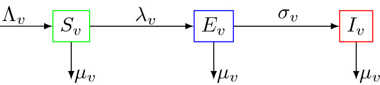
Model flow diagram of the mosquito component of the model

The model

The variables and parameters values of the model are presented in the following Tables 1 and 2, respectively.

Table 1.

Variable of model

Variable	Description
Humans
$S_e$	Population of susceptible humans under 5 years old
$V_e$	Population of vaccinated humans under 5 years old
$E_e$	Population of infected humans under 5 years old
$I_e$	Population of infectious humans under 5 years old
$S_a$	Population of humans over 5 years old
$E_a$	Population of infected humans over 5 years old
$I_a$	Population of infectious humans over 5 years old
$R_a$	Population of recovered humans over 5 years old
Mosquitoes
$S_v$	Population of susceptible mosquitoes
$E_v$	Population of infected mosquitoes
$I_v$	Population of infectious mosquitoes

Table 2.

Model parameter

Parameter	Description
$b_1$	Average biting rate of mosquitoes on susceptible humans over 5 years old
$b_2$	Average biting rate of mosquitoes on susceptible humans under 5 years old
${\mathrm{\Lambda }}_e$	Recruitment rate of humans under 5 years old
${\sigma }_e$	Progression rate from exposed to infectious for humans under 5 years old
${\omega }_e$	Recovery rate of infectious humans under 5 years old
${\vartheta }_e$	Vaccination rate of susceptible humans under 5 years old
$\epsilon$	Vaccination efficacy
${\beta }_e$	Probability of infection of susceptible humans under 5 years old per mosquito bite
$d_1$	Disease-induced mortality rate for humans under 5 years old
$\xi$	Maturation rate for human under 5 years old
${\sigma }_a$	Progression rate from exposed to infectious for humans over 5 years old
${\omega }_a$	Recovery rate of infectious humans over 5 years old
u	Proportion of infectious humans over 5 years old that becomes immune
${\beta }_a$	Probability of infection of susceptible humans over 5 years old per mosquito bite
${\delta }_a$	Rate of loss of natural immunity for humans over 5 years old
${\mu }_h$	Natural death rate of humans
$d_2$	Disease-induced mortality rate for humans over 5 years old
${\mathrm{\Lambda }}_v$	Birth rate of adult mosquitoes
${\sigma }_v$	Progression rate from exposed to infectious mosquitoes
${\beta }_v$	Probability of infection of susceptible vectors per mosquito bite of the infected human
${\mu }_v$	Natural death rate of mosquitoes

Based on our model description and assumptions, we establish the following system of non-linear ordinary differential equations.

$$\begin{array}{c}\hfill \left\{\begin{array}{c}{S}_e^{\prime }={\mathrm{\Lambda }}_e+{\omega }_e{I}_e-({\lambda }_e+{\vartheta }_e+\xi +{\mu }_h)S_e,\hfill \\ V_e^{\prime }={\vartheta }_e{S}_e-((1-\epsilon ){\lambda }_e+{\mu }_h)V_e,\hfill \\ S_a^{\prime }=\xi S_e+u{\omega }_a{I}_a+{\delta }_a{R}_a-({\lambda }_a+{\mu }_h)S_a,\hfill \\ E_e^{\prime }={\lambda }_e(S_e+(1-\epsilon )V_e)-({\sigma }_e+{\mu }_h)E_e,\hfill \\ E_a^{\prime }={\lambda }_a{S}_a-({\sigma }_a+{\mu }_h)E_a,\hfill \\ I_e^{\prime }={\sigma }_e{E}_e-({\omega }_e+{\mu }_h+d_1)I_e,\hfill \\ I_a^{\prime }={\sigma }_a{E}_a-({\omega }_a+{\mu }_h+d_2)I_a,\hfill \\ R_a^{\prime }=(1-u){\omega }_a{I}_a-({\delta }_a+{\mu }_h)R_a,\hfill \\ S_v^{\prime }={\mathrm{\Lambda }}_v-({\lambda }_v+{\mu }_v)S_v,\hfill \\ E_v^{\prime }={\lambda }_v{S}_v-({\sigma }_v+{\mu }_v)E_v,\hfill \\ I_v^{\prime }={\sigma }_v{E}_v-{\mu }_v{I}_v,\hfill \end{array}\right)\end{array}$$ 1

with initial conditions

$$\begin{array}{c}\hfill (S_e(0),V_e(0),S_a(0),S_v(0),E_e(0),E_a(0),E_v(0),I_e(0),I_a(0),I_v(0),R_a(0))\in {\mathbb{R}}_{+}^{11}\end{array}.$$

The forces of infections are given by

$$\begin{array}{c}\hfill {\lambda }_e={\displaystyle \frac{b_2{\beta }_e}{N_h}}{I}_v,{\lambda }_a={\displaystyle \frac{b_1{\beta }_a}{N_h}}{I}_v,{\lambda }_v={\displaystyle \frac{{\beta }_v[b_2{I}_e+b_1{I}_a]}{N_h}}.\end{array}$$

Model analysis

Existence, uniqueness and positivity of solutions

The functions on the right-hand side of the system (1) are Lipschitz continuous, therefore by Picard’s existence Theorem, the system (1) has a solution.

Theorem 3.1

The solutions of the model system (1) with non-negative initial conditions are all non-negative.

Proof

Assume that there exists a time $\tilde{t}$ such that $S_e(\tilde{t})=0,$ $S_e^{\prime }(\tilde{t})<0,$ $S_e(t)>0,$ $S_a(t)>0,$ $I_e(t)>0,$ $I_a(t)>0,$ $V_e(t)>0,$ $E_e(t)>0,$ $E_a(t)>0,$ $E_v(t)>0,$ $R_a(t)>0,$ $S_v(t)>0,$ $I_v(t)>0,$ for $0<t<\tilde{t}.$ From the first equation of (1), we have

$$\begin{array}{c}\hfill {\displaystyle \frac{d{S}_e(\tilde{t})}{\mathit{dt}}}={\mathrm{\Lambda }}_e+w_{e}I>0.\end{array}$$

This contradicts the assumption that $S_e^{\prime }(\tilde{t})<0.$ Therefore S(t) is positive.

Similarly, $S_a(t),$ $I_e(t),$ $I_a(t),$ $V_e(t),$ $E_e(t),$ $E_a(t),$ $E_v(t),$ $R_a(t),$ $S_v(t),$ $I_v(t)$ are all positive. $\square$

Theorem 3.2

Solutions the model system (1) are bounded in the invariant region

$$\begin{array}{c}\hfill \mathrm{\Omega }=\left\{{\displaystyle (S_e,S_a,I_e,I_a,V_e,E_e,E_a,E_v,R_a,S_v,I_v,)\in {\mathbb{R}}_{+}^{11}:N_h(t)\le \frac{{\mathrm{\Lambda }}_e}{{\mu }_h},N_v(t)\le {\displaystyle \frac{{\mathrm{\Lambda }}_v}{{\mu }_v}}}\right\}.\end{array}$$

Proof

Given $N_h(t)=S_a(t)+S_e(t)+I_e(t)+I_a(t)+V_e(t)+E_e(t)+E_a(t)+R_a(t)$ and $N_v(t)=+E_v(t)+S_v(t)+I_v(t).$

$$\begin{array}{cc}\hfill {\displaystyle \frac{d{N}_h}{\mathit{dt}}}=& ({\mathrm{\Lambda }}_e-{\mu }_h{N}_h)-(d_1{I}_e+d_2{I}_a),\hfill \\ \hfill \le & {\mathrm{\Lambda }}_e-{\mu }_h{N}_h.\hfill \end{array}$$

Solving the differential inequality, we obtain

$$\begin{array}{c}\hfill N_h(t)\le {\displaystyle \frac{{\mathrm{\Lambda }}_e}{{\mu }_h}}+\left({\displaystyle \frac{{\mathrm{\Lambda }}_e}{{\mu }_h}},-,N_h,(0)\right)exp(-{\mu }_{h}t).\end{array}$$

Therefore,

$$\begin{array}{c}\hfill \underset{t⟶\infty }{lim\; sup}{N}_h(t)={\displaystyle \frac{{\mathrm{\Lambda }}_e}{{\mu }_h}}.\end{array}$$

Since $N_h(t)=S_a(t)+S_e(t)+I_e(t)+I_a(t)+V_e(t)+E_e(t)+E_a(t)+R_a(t),$ it follows that $S_e(t)\le {\displaystyle \frac{{\mathrm{\Lambda }}_e}{{\mu }_h}},$   $S_a(t)\le {\displaystyle \frac{{\mathrm{\Lambda }}_e}{{\mu }_h}},$ $E_e(t)\le {\displaystyle \frac{{\mathrm{\Lambda }}_e}{{\mu }_h}},$   $E_a(t)\le {\displaystyle \frac{{\mathrm{\Lambda }}_e}{{\mu }_h}},$   $I_e(t)\le {\displaystyle \frac{{\mathrm{\Lambda }}_e}{{\mu }_h}},$   $I_a(t)\le {\displaystyle \frac{{\mathrm{\Lambda }}_e}{{\mu }_h}},$   $V_e(t)\le {\displaystyle \frac{{\mathrm{\Lambda }}_e}{{\mu }_h}},$   $R_a(t)\le {\displaystyle \frac{{\mathrm{\Lambda }}_e}{{\mu }_h}}.$

$$\begin{array}{cc}\hfill {\displaystyle \frac{d{N}_v}{\mathit{dt}}}=& {\mathrm{\Lambda }}_v-{\mu }_v{N}_v.\hfill \end{array}$$

Thus, the solution of this differential equation is

$$\begin{array}{c}\hfill N_v(t)={\displaystyle \frac{{\mathrm{\Lambda }}_v}{{\mu }_v}}-\left({\displaystyle \frac{{\mathrm{\Lambda }}_v}{{\mu }_v}},-,N_v,(0)\right)exp(-{\mu }_{v}t).\end{array}$$

Therefore,

$$\begin{array}{c}\hfill \underset{t⟶\infty }{lim\; sup}{N}_v(t)={\displaystyle \frac{\mathrm{\Lambda }}{{\mu }_v}},\end{array}$$

and it follows that $S_v(t)\le {\displaystyle \frac{{\mathrm{\Lambda }}_v}{{\mu }_v}},$  $E_v(t)\le {\displaystyle \frac{{\mathrm{\Lambda }}_v}{{\mu }_v}}$  and  $I_v(t)\le {\displaystyle \frac{{\mathrm{\Lambda }}_v}{{\mu }_v}}.$ $\square$

In what follows, for simplicity, let $k=({\vartheta }_e+\xi +{\mu }_h),$ $k_0=({\sigma }_e+{\mu }_h),$ $k_1=({\sigma }_a+{\mu }_h),$ $k_2=({\omega }_e+{\mu }_h+d_1),$ $k_3=({\omega }_a+{\mu }_h+d_2),$ $k_4=({\mu }_h+{\delta }_a),$ and  $k_5=({\sigma }_v+{\mu }_v)$.

Disease-free equilibrium and basic reproduction number

We first show the existence of a trivial disease-free equilibrium (DFE) for our malaria model without control (MMWC) which is used in computing the basic reproduction number. The MMWC DFE is

$$\begin{array}{c}\hfill {\displaystyle {\mathcal{M}}^0=\left(S_e^0,,,V_e^0,,,S_a^0,,,S_v^0,,,E_e^0,,,E_a^0,,,E_v^0,,,I_e^0,,,I_a^0,,,I_v^0,,,R_a^0\right)=\left({\displaystyle \frac{{\mathrm{\Lambda }}_e}{k}},,,{\displaystyle \frac{{\vartheta }_e{\mathrm{\Lambda }}_e}{{\mu }_{h}k}},,,{\displaystyle \frac{\xi {\mathrm{\Lambda }}_e}{{\mu }_{h}k}},,,{\displaystyle \frac{{\mathrm{\Lambda }}_v}{{\mu }_v}},,,0,,,0,,,0,,,0,,,0,,,0,,,0\right).}\end{array}$$

To calculate the basic reproduction number, we apply the next generation method in van den Driessche and Watmough (2002). We now have that

$$\begin{array}{cc}\hfill F=& \left(\begin{array}{c}{\displaystyle {\lambda }_e(S_e+(1-\epsilon )V_e)}\\ {\displaystyle {\lambda }_a{S}_a}\\ {\displaystyle {\lambda }_v{S}_v}\\ {\displaystyle 0}\\ {\displaystyle 0}\\ {\displaystyle 0}\end{array}\right),\text{and}V=\left(\begin{array}{c}{\displaystyle k_0{E}_e}\\ {\displaystyle k_1{E}_a}\\ {\displaystyle k_5{E}_v}\\ {\displaystyle k_2{I}_e-{\sigma }_e{E}_e}\\ {\displaystyle k_3{I}_a-{\sigma }_a{E}_a}\\ {\displaystyle {\mu }_v{I}_v-{\sigma }_v{E}_v}\end{array}\right)\hfill \\ \hfill \mathcal{F}=& \left(\begin{array}{cccccc}{\displaystyle 0}& 0& 0& 0& 0& {\displaystyle \frac{{\beta }_e{b}_2\left(k,+,(1-\epsilon ),{\vartheta }_e\right)}{k}}\\ {\displaystyle 0}& 0& 0& 0& 0& {\displaystyle \frac{{\beta }_a{b}_1\xi }{k}}\\ {\displaystyle 0}& 0& 0& {\displaystyle \frac{{\beta }_v{b}_2{\mathrm{\Lambda }}_v{\mu }_h}{{\mu }_v{\mathrm{\Lambda }}_e}}& {\displaystyle \frac{{\beta }_v{b}_1{\mathrm{\Lambda }}_v{\mu }_h}{{\mu }_v{\mathrm{\Lambda }}_e}}& 0\\ {\displaystyle 0}& 0& 0& 0& 0& 0\\ {\displaystyle 0}& 0& 0& 0& 0& 0\\ {\displaystyle 0}& 0& 0& 0& 0& 0\end{array}\right),\text{and}\mathcal{V}=\left(\begin{array}{cccccc}{\displaystyle k_0}& 0& 0& 0& 0& 0\\ {\displaystyle 0}& k_1& 0& 0& 0& 0\\ {\displaystyle 0}& 0& k_5& 0& 0& 0\\ {\displaystyle -{\sigma }_e}& 0& 0& k_2& 0& 0\\ {\displaystyle 0}& -{\sigma }_a& 0& 0& k_3& 0\\ {\displaystyle 0}& 0& -{\sigma }_v& 0& 0& {\mu }_v\end{array}\right).\hfill \end{array}$$

Hence,

$$\begin{array}{c}\hfill {\displaystyle {\mathcal{R}}_C^m=\sqrt{{\displaystyle \frac{{\mathrm{\Lambda }}_v{\beta }_v{\mu }_h{\sigma }_v\left[b_2^2,{\beta }_e,k_1,k_3,{\sigma }_e,({\mu }_h+(1-\epsilon ){\vartheta }_e),+,b_1^2,{\beta }_a,k_0,k_2,{\sigma }_a,\xi \right]}{{\mathrm{\Lambda }}_e{\mu }_v^{2}k{k}_0{k}_1{k}_2{k}_5}}}·}\end{array}$$

Global stability of the DFE

To prove the global asymptotically stability (GAS) of the DFE, we use the approach described in Castillo-Chavez et al. (2002). We then re-write the malaria model (1) as follows

$$\begin{array}{c}\hfill \left\{\begin{array}{c}{\displaystyle \frac{\mathit{dX}}{\mathit{dt}}}=F\left(X,,,I\right),\hfill \\ \hfill \\ {\displaystyle \frac{\mathit{dI}}{\mathit{dt}}}=\mathcal{G}\left(X,,,I\right),\mathcal{G}\left(X,,,0\right)=0,\hfill \end{array}\right)\end{array}$$ 2

in which $X=\left(S_e,,,V_e,,,S_a,,,R_a,,,S_v\right)\in {\mathbb{R}}^5$ and $I=\left(E_e,,,E_a,,,E_v,,,I_e,,,I_a,,,I_v\right)\in {\mathbb{R}}^6.$ We note here that X and I represents the classes of the un-infectious and infectious individuals, respectively. Let the DFE from Sect. 3.2 be

$$\begin{array}{c}\hfill {\displaystyle {\mathcal{M}}^0=(X_0,0)=\left(S_e^0,,,V_e^0,,,S_a^0,,,R_a^0,,,S_v^0,,,E_e^0,,,E_a^0,,,E_v^0,,,I_e^0,,,I_a^0,,,I_v^0\right)=\left({\displaystyle \frac{{\mathrm{\Lambda }}_e}{k}},,,{\displaystyle \frac{{\vartheta }_e{\mathrm{\Lambda }}_e}{{\mu }_{h}k}},,,{\displaystyle \frac{\xi {\mathrm{\Lambda }}_e}{{\mu }_{h}k}},,,0,,,{\displaystyle \frac{{\mathrm{\Lambda }}_v}{{\mu }_v}},,,0,,,0,,,0,,,0,,,0,,,0\right).}\end{array}$$

For the model to be GAS at ${\mathcal{M}}^0,$ it needs to satisfy the following conditions from Castillo-Chavez et al. (2002), which are

$({\mathcal{C}}_1)$

Local stability is guaranteed at ${\mathcal{M}}^0$ whenever $({\mathcal{R}}_C^m<1.$

${\mathcal{C}}_1)$

At ${\displaystyle \frac{\mathit{dX}}{\mathit{dt}}}=F(X_0,0)$ the DFE is globally asymptotically stable.

$({\mathcal{C}}_3)$

$\mathcal{G}(X,I)=\mathcal{A}I-\widehat{\mathcal{G}}(X,I),\widehat{\mathcal{G}}(X,I)\ge 0$ for $(X,I)\in \mathrm{\Omega },$ where $\mathcal{A}={\mathcal{D}}_I\mathcal{G}({\mathcal{M}}^0)$ is an Metzler matrix, and $\mathrm{\Omega }$ is the model biologically feasible region defined earlier.

Theorem 3.3

If the disease-induced death rate is zero $(d_1=d_2=0)$, then the disease-free equilibrium ${\mathcal{M}}^0$ is globally asymptotically (GAS) stable when ${\mathcal{R}}_C^m<1$.

Proof

To prove that the DFE is GAS when ${\mathcal{R}}_C^m<1$, we have to verify the conditions ${\mathcal{C}}_1$ to ${\mathcal{C}}_3.$

Using the approach in van den Driessche and Watmough (2002), we obtain that the DFE ${\mathcal{M}}^0$ is LAS when ${\mathcal{R}}_C^m<1$, so the condition ${\mathcal{C}}_1$ is verified.

Next, we re-write the model system (1) in the form given in (2) as

$$\begin{array}{c}\hfill {\displaystyle \frac{\mathit{dX}}{\mathit{dt}}}=F(X,I)=\left(\begin{array}{c}{\displaystyle {\mathrm{\Lambda }}_e+{\omega }_e{I}_e-({\lambda }_e+k)S_e}\\ {\displaystyle {\vartheta }_e{S}_e-((1-\epsilon ){\lambda }_e+{\mu }_h)V_e}\\ {\displaystyle \xi S_e+u{\omega }_a{I}_a+{\delta }_a{R}_a-({\lambda }_a+{\mu }_h)S_a}\\ {\displaystyle {\mathrm{\Lambda }}_v-({\lambda }_v+{\mu }_v)S_v,}\\ {\displaystyle (1-u){\omega }_a{I}_a-k_4{R}_a}\\ \end{array}\right),\text{and}{\displaystyle \frac{\mathit{dI}}{\mathit{dt}}}=G(X,I)=\left(\begin{array}{c}{\displaystyle {\lambda }_e(S_e+(1-\epsilon )V_e)-k_0{E}_e}\\ {\displaystyle {\lambda }_a{S}_a-k_1{E}_a}\\ {\displaystyle {\lambda }_v{S}_v-k_5{E}_v}\\ {\displaystyle {\sigma }_e{E}_e-k_2{I}_e}\\ {\displaystyle {\sigma }_a{E}_a-k_3{I}_a}\\ {\displaystyle {\sigma }_v{E}_v-{\mu }_v{I}_v}\end{array}\right).\end{array}$$ 3

$$\begin{array}{c}\hfill {\displaystyle \frac{\mathit{dX}}{\mathit{dt}}}=F(X_0,0)\iff \left\{\begin{array}{c}{\dot{S}}_e={\mathrm{\Lambda }}_e-k{S}_e,\hfill \\ {\dot{V}}_e={\vartheta }_e{S}_e-{\mu }_h{V}_e,\hfill \\ {\dot{S}}_a=\xi S_e+{\delta }_a{R}_a-{\mu }_h{S}_a,\hfill \\ {\dot{R}}_a=-k_4{R}_a,\hfill \\ {\dot{S}}_v=-{\mu }_v{S}_v.\hfill \end{array}\right)\end{array}$$ 4

This equation has a unique equilibrium point $\left({\displaystyle \frac{{\mathrm{\Lambda }}_e}{k}},,,{\displaystyle \frac{{\vartheta }_e{\mathrm{\Lambda }}_e}{{\mu }_{h}k}},,,{\displaystyle \frac{\xi {\mathrm{\Lambda }}_e}{{\mu }_{h}k}},,,0,,,{\displaystyle \frac{{\mathrm{\Lambda }}_v}{{\mu }_v}}\right)$ which is globally asymptotically stable. Therefore, the condition ${\mathcal{C}}_2$ is satisfied.

Linearizing the second matrix in equation (3) gives the Metzler Matrix

$$\begin{array}{c}\hfill \mathcal{A}={\mathcal{D}}_Z\mathcal{G}({\mathcal{M}}^0)=\left(\begin{array}{cccccc}{\displaystyle -k_0}& 0& 0& 0& 0& {\displaystyle \frac{{\beta }_e{b}_2}{N_h^0}}(S_e^0+(1-\epsilon )V_e^0)\\ {\displaystyle 0}& -k_1& 0& 0& 0& {\displaystyle \frac{{\beta }_a{b}_1}{N_h^0}}{S}_a^0\\ {\displaystyle 0}& 0& -k_5& {\displaystyle \frac{{\beta }_v{b}_1}{N_h^0}}{S}_v^0& {\displaystyle \frac{{\beta }_v{b}_2}{N_h^0}}{S}_v^0& 0\\ {\displaystyle {\sigma }_e}& 0& 0& -k_2& 0& 0\\ {\displaystyle 0}& {\sigma }_a& 0& 0& -k_3& 0\\ {\displaystyle 0}& 0& {\sigma }_v& 0& 0& -{\mu }_v\\ \end{array}\right).\end{array}$$

Computing $\widehat{\mathcal{G}}(X,Z)$ and after some algebraic simplifications, we have

$$\begin{array}{c}\hfill \widehat{\mathcal{G}}(X,I)=\mathcal{A}I-\mathcal{G}(X,I)=\left(\begin{array}{c}{\displaystyle {\beta }_e{b}_2{I}_v\left[{\displaystyle \frac{S_e^0}{N_h^0}},-,{\displaystyle \frac{S_e}{N_h}},+,(1-\epsilon ),\left({\displaystyle \frac{V_e^0}{N_h^0}},-,{\displaystyle \frac{V_e}{N_h}}\right)\right]}\\ {\displaystyle {\beta }_a{b}_1{I}_v\left[{\displaystyle \frac{S_a^0}{N_h^0}},-,{\displaystyle \frac{S_a}{N_h}}\right]}\\ {\displaystyle {\beta }_v\left(b_2,I_e,+,b_1,I_a\right)\left[{\displaystyle \frac{S_v^0}{N_h^0}},-,{\displaystyle \frac{S_v}{N_h}}\right]}\\ {\displaystyle 0}\\ {\displaystyle 0}\\ {\displaystyle 0}\\ \end{array}\right).\end{array}$$

Thus,

$$\begin{array}{c}\hfill \widehat{\mathcal{G}}(X,I)\ge \left(\begin{array}{c}{\displaystyle {\beta }_e{b}_2{I}_v\left[S_e^0,+,(1-\epsilon ),V_e^0\right]\left({\displaystyle \frac{1}{N_h^0}},-,{\displaystyle \frac{1}{N_h}}\right)}\\ \\ {\displaystyle {\beta }_a{b}_1{I}_v{S}_a^0\left({\displaystyle \frac{1}{N_h^0}},-,{\displaystyle \frac{1}{N_h}}\right)}\\ {\displaystyle {\beta }_v\left(b_2,I_e,+,b_1,I_a\right)S_v^0\left({\displaystyle \frac{1}{N_h^0}},-,{\displaystyle \frac{1}{N_h}}\right)}\\ {\displaystyle 0}\\ {\displaystyle 0}\\ {\displaystyle 0}\\ \end{array}\right).\end{array}$$

Since $\left({\displaystyle \frac{1}{N_h^0}},-,{\displaystyle \frac{1}{N_h}}\right)={\displaystyle \frac{N_h-N_h^0}{N_h{N}_h^0}}$, when $d_1=d_2=0$, $N_h(t)-N_h^0=\left({\displaystyle \frac{{\mathrm{\Lambda }}_e}{{\mu }_h}},-,N_h,(0)\right)exp(-{\mu }_{h}t)$ is positive, and we obtain $\widehat{\mathcal{G}}(X,I)\ge 0$. The condition ${\mathcal{C}}_3$ is satisfied. We can conclude that if $d_1=d_2=0$, then, the DFE is GAS when ${\mathcal{R}}_C^m<1$.

$\square$

Remark 3.1

When the disease-induced death rate is not zero, the condition ${\mathcal{R}}_C^m<1$ is not sufficient for the global stability of disease-free equilibrium and the phenomenon of backward bifurcation may occur. In this case, to mitigate the spread of the disease, it is necessary to reduce ${\mathcal{R}}_C^m$ to less than another threshold, say ${\mathcal{R}}_C^{\#}<{\mathcal{R}}_C^m<1$.

Existence of the endemic equilibrium

By setting the left-hand side of the model system (1) to zero and solving it, we obtain the endemic equilibrium point as follows:

$$\begin{array}{c}\hfill S_e^{\ast }={\displaystyle \frac{\left({\mathrm{\Lambda }}_v^{\ast },b_2,{\beta }_e,(1-\epsilon ),{\lambda }_v^{\ast },{\sigma }_v,+,N_h^{\ast },k_5,{\lambda }_v^{\ast },{\mu }_h,{\mu }_v,+,N_h^{\ast },k_5,{\mu }_h,{\mu }_v^2\right){\mathrm{\Lambda }}_e{N}_h^{\ast }{k}_0{k}_2{k}_5\left({\lambda }_v^{\ast },+,{\mu }_v\right){\mu }_v}{{\mathrm{\Lambda }}_e{N}_h^{\ast }{b}_2{\beta }_e{\sigma }_v{\lambda }_v^{\ast }\left[k_5,{\mu }_v,({\lambda }_v^{\ast }+{\mu }_v),((1-\epsilon )(k{k}_0{k}_2-{\omega }_e{\sigma }_e{\vartheta }_e)+{\mu }_h(k_0{k}_2-{\omega }_e{\sigma }_e))\right]+k_6}},\end{array}$$ 5

where   $k_6={({\mathrm{\Lambda }}_v{b}_2{\beta }_e{\sigma }_v{\lambda }_v)}^2(1-\epsilon )(k_0{k}_2-{\omega }_e{\sigma }_e)+N_h^{\ast }k{k}_0{k}_2{k}_5{\mu }_h{\mu }_v^2{({\lambda }_v+{\mu }_v)}^2$, and $N_h^{\ast }={\displaystyle \frac{{\mathrm{\Lambda }}_e}{{\mu }_h}}.$

We also have

$$\begin{array}{c}\hfill \begin{array}{cccc}{S}_v^{\ast }={\displaystyle \frac{{\mathrm{\Lambda }}_v}{{\lambda }_v+{\mu }_v}},& E_v^{\ast }={\displaystyle \frac{{\lambda }_v{S}_v^{\ast }}{k_5}},& I_v^{\ast }={\displaystyle \frac{{\sigma }_v{E}_v^{\ast }}{{\mu }_v}},& \\ \\ {\lambda }_e^{\ast }={\displaystyle \frac{b_2{\beta }_e{I}_v^{\ast }}{N_h^{\ast }}},& V_e^{\ast }={\displaystyle \frac{\vartheta S_e^{\ast }}{(1-\epsilon ){\lambda }_e^{\ast }+m{u}_h)}},& E_e^{\ast }={\displaystyle \frac{{\lambda }_e^{\ast }(S_e^{\ast }+(1-\epsilon )V_e^{\ast })}{k_0}},& I_e={\displaystyle \frac{{\sigma }_e{E}_e^{\ast }}{k_2}}\end{array},\end{array}$$ 6

$$\begin{array}{c}\hfill S_a^{\ast }={\displaystyle \frac{{\mathrm{\Lambda }}_e{S}_e^{\ast }{k}_1{k}_3{k}_4{k}_5\xi ({\lambda }_v^{\ast }+{\mu }_v)}{{\mu }_v\left[{\mathrm{\Lambda }}_e,k_1,k_3,k_4,k_5,{\mu }_v,({\lambda }_v^{\ast }+{\mu }_v),+,{\mathrm{\Lambda }}_v,b_1,{\beta }_a,{\sigma }_v,{\lambda }_v^{\ast },(k_1{k}_3{k}_4-{\delta }_a{\omega }_a{\sigma }_a-u{\omega }_a{\sigma }_a{\mu }_h)\right]}},\end{array}$$ 7

$$\begin{array}{c}\hfill \begin{array}{cccc}{\lambda }_a^{\ast }={\displaystyle \frac{b_1{\beta }_a{I}_v^{\ast }}{N_h^{\ast }}},& E_a^{\ast }={\displaystyle \frac{{\lambda }_a^{\ast }{S}_a^{\ast }}{k_1}},& I_a^{\ast }={\displaystyle \frac{{\sigma }_a{E}_a^{\ast }}{k_3}},& R_a^{\ast }={\displaystyle \frac{(1-u){\omega }_a{I}_a^{\ast }}{k_4}}.\end{array}\end{array}$$ 8

Substituting the expressions for $I_a^{\ast }$ and $I_e^{\ast }$ into the expression for ${\lambda }_v,$ we obtain the polynomial

$$\begin{array}{c}\hfill a_3{\lambda }_v^{\ast 3}+a_2{\lambda }_v^{\ast 2}+a_1{\lambda }_v^{\ast }+a_0,\end{array}$$ 9

where the expressions of $a_0,a_1,a_2$ and $a_3$ are given in the Appendix.

Because the model monitors human populations, all associated state variables should be non-negative for all time $t\ge 0$. We therefore use Descarte’s rule of signs to discuss the existence of possible positive roots of Eq. (9). The results are summarized in Table 3.

Table 3.

Number of possible positive roots of equation (9) using Descarte’s rule of signs

Case	$a_3$	$a_2$	$a_1$	$a_0$	Possible positive roots	${\mathcal{R}}_C^m$ Condition
(1)	$+$	+	+	−	1	${\mathcal{R}}_C^m<1$
(2)	$+$	+	+	$+$	0	${\mathcal{R}}_C^m>1$
(3)	$+$	+	−	−	1	${\mathcal{R}}_C^m<1$
(4)	$+$	+	−	$+$	0 or 2	${\mathcal{R}}_C^m>1$
(5)	$+$	−	+	−	1 or 3	${\mathcal{R}}_C^m<1$
(6)	$+$	−	+	$+$	0 or 2	${\mathcal{R}}_C^m>1$
(7)	$+$	−	−	−	1	${\mathcal{R}}_C^m<1$
(8)	$+$	−	−	$+$	0 or 2	${\mathcal{R}}_C^m>1$
(9)	−	+	+	−	0 or 2	${\mathcal{R}}_C^m<1$
(10)	−	+	+	$+$	1	${\mathcal{R}}_C^m>1$
(11)	−	+	−	$-$	0 or 2	${\mathcal{R}}_C^m<1$
(12)	−	+	−	$+$	1 or 3	${\mathcal{R}}_C^m>1$
(13)	−	−	+	−	0 or 2	${\mathcal{R}}_C^m<1$
(14)	−	−	+	$+$	1	${\mathcal{R}}_C^m>1$
(15)	−	−	−	−	0	${\mathcal{R}}_C^m<1$
(16)	−	−	−	$+$	1	${\mathcal{R}}_C^m>1$

The following remark summarizes the results in Table 3

Remark 3.2

• If all the coefficients of the polynomial (9) have the same signs, then the model system (1) has no endemic equilibrium point,

• If ${\mathcal{R}}_C^m\ne 1,$ then the system has zero, one, two or three endemic equilibrium points,

• If ${\mathcal{R}}_C^m=1,$ then the system has either zero, one or two endemic equilibrium points.

The last two conditions above imply that the model system (1) could exhibit the phenomenon of backward/subcritical bifurcation, when a stable DFE co-exists with a stable endemic equilibrium. This is an epidemiological situation in which the classical requirement of having the basic reproduction number less than unity although necessary is not sufficient to eliminate the disease.

Optimal control model

The application of optimal control enables us to forecast or choose the best scenario that if well implemented could help mitigate the spread of the disease. Thus, to investigate the potential impact of the implemented intervention measures, the following control variables are incorporated into the model system (1):

• $c_1(t)$ representing the use of personal protection measures to prevent mosquitoes bites during the day and the night such as the use of insecticide-treated nets, application of repellents to skin or spraying of insecticides,

• $c_2(t)$ representing the treatment, and

• $c_3(t)$ representing the use of vaccination to prevent malaria,

as follows

$$\begin{array}{c}\hfill \left\{\begin{array}{c}{S}_e^{\prime }={\mathrm{\Lambda }}_e+c_2{\omega }_e{I}_e-((1-c_1){\lambda }_e+c_3{\vartheta }_e+\xi +{\mu }_h)S_e,\hfill \\ \hfill \\ V_e^{\prime }=c_3{\vartheta }_e{S}_e-((1-c_1)(1-\epsilon ){\lambda }_e+{\mu }_h)V_e,\hfill \\ \hfill \\ S_a^{\prime }=\xi S_e+(1-p)c_2{\omega }_a{I}_a+{\delta }_a{R}_a-((1-c_1){\lambda }_a+{\mu }_h)S_a,\hfill \\ \hfill \\ E_e^{\prime }=(1-c_1){\lambda }_e(S_e+(1-\epsilon )V_e)-({\sigma }_e+{\mu }_h)E_e,\hfill \\ \hfill \\ E_a^{\prime }=(1-c_1){\lambda }_a{S}_a-({\sigma }_a+{\mu }_h)E_a,\hfill \\ \hfill \\ I_e^{\prime }={\sigma }_e{E}_e-(c_2{\omega }_e+{\mu }_h+d_1)I_e,\hfill \\ \hfill \\ I_a^{\prime }={\sigma }_a{E}_a-(c_2{\omega }_a+{\mu }_h+d_2)I_a,\hfill \\ \hfill \\ R_a^{\prime }=p{c}_2{\omega }_a{I}_a-({\mu }_h+{\delta }_a)R_a,\hfill \\ \hfill \\ S_v^{\prime }={\mathrm{\Lambda }}_v-((1-c_1){\lambda }_v+{\mu }_v)S_v,\hfill \\ \hfill \\ E_v^{\prime }=(1-c_1){\lambda }_v{S}_v-({\sigma }_v+{\mu }_v)E_v,\hfill \\ \hfill \\ I_v^{\prime }={\sigma }_v{E}_v-{\mu }_v{I}_v.\hfill \end{array}\right)\end{array}$$ 10

Consider the following quadratic objective functional which measures the cost of the control. This cost includes the above interventions. The the nonlinear objective function is

$$\begin{array}{c}\hfill J\left(c_1,,,c_2,,,c_3\right)={\int }_0^T\left[A_1,E_e,(t),+,A_2,E_a,(t),+,A_3,I_e,(t),+,A_4,I_{(},t)+,A_5,N_v,(t),+,\frac{w_1}{2},c_1^2,+,\frac{w_2}{2},c_2^2,+,\frac{w_3}{2},c_3^2\right]dt,\end{array}$$ 11

where T is the final time, $A_i,i=1,\cdots ,5$ are positive weight constants, $N_v=S_v++E_v+I_v$ and $w_i,i=1,\cdots ,3$ are weight constants for the strategies and treatments against proliferation of malaria. The fact that the controls are linearly in (10) and quadratic in the objective functional allows the Hamiltonian associated to the optimal control problem to be maximized. Therefore, we seek to find, using the Pontryagin Maximum Principle (Pontryagin et al. 1986), an optimal control $(c_1^{\ast },c_2^{\ast },c_3^{\ast })\in U$ satisfying (10), such that

$$\begin{array}{c}\hfill J\left(c_1^{\ast },,,c_2^{\ast },,,c_3^{\ast }\right)=min\left\{J,\left(c_1,,,c_2,,,c_3\right),|,(c_1,c_2,c_3),\in ,U\right\}.\end{array}$$ 12

The associated pseudo-Hamiltonian is

$$\begin{array}{cc}\hfill {\displaystyle H=}& {\displaystyle A_1{E}_e(t)+A_2{E}_a(t)+A_3{I}_e(t)+A_4{I}_a(t)+A_5{N}_v(t)+\frac{w_1}{2}{c}_1^2+\frac{w_2}{2}{c}_2^2+\frac{w_3}{2}{c}_3^2}\hfill \\ \hfill & {\displaystyle +{\xi }_1\left[{\mathrm{\Lambda }}_e,+,c_2,{\omega }_e,I_e,-,((1-c_1){\lambda }_e+c_3{\vartheta }_e+\xi +{\mu }_h),S_e\right]}\hfill \\ \hfill & {\displaystyle +{\xi }_2\left[c_3,{\vartheta }_e,S_e,-,((1-c_1)(1-\epsilon ){\lambda }_e+{\mu }_h),V_e\right)}\hfill \\ \hfill & {\displaystyle +{\xi }_3\left[\xi ,S_e,+,(1-u),c_2,{\omega }_a,I_a,+,{\delta }_a,R_a,-,((1-c_1){\lambda }_a+{\mu }_h),S_a,,\right]}\hfill \\ \hfill & {\displaystyle +{\xi }_4\left[(1-c_1),{\lambda }_e,(S_e+(1-\epsilon )V_e),-,({\sigma }_e+{\mu }_h),E_e\right]}\hfill \\ \hfill & {\displaystyle +{\xi }_5\left[(1-c_1),{\lambda }_a,S_a,-,({\sigma }_a+{\mu }_h),E_a\right]}\hfill \\ \hfill \\ \hfill & {\displaystyle +{\xi }_6\left[{\sigma }_e,E_e,-,(c_2{\omega }_e+{\mu }_h+d_1),I_e\right]}\hfill \\ \hfill \\ \hfill & {\displaystyle +{\xi }_7\left[{\sigma }_a,E_a,-,(c_2{\omega }_a+{\mu }_h+d_2),I_a\right]}\hfill \\ \hfill \\ \hfill & {\displaystyle +{\xi }_8\left[u,c_2,{\omega }_a,I_a,-,({\mu }_h+{\delta }_a),R_a\right]}\hfill \\ \hfill \\ \hfill & {\displaystyle +{\xi }_9\left[{\mathrm{\Lambda }}_v,-,((1-c_1){\lambda }_v+{\mu }_v),S_v\right]}\hfill \\ \hfill \\ \hfill & {\displaystyle +{\xi }_{10}\left[(1-c_1),{\lambda }_v,S_v,-,({\sigma }_v+{\mu }_v),E_v\right]}\hfill \\ \hfill \\ \hfill & {\displaystyle +{\xi }_{11}\left[{\sigma }_v,E_v,-,{\mu }_v,I_v\right],}\hfill \end{array}$$ 13

where the ${\xi }_1,{\xi }_2,{\xi }_3,{\xi }_4,{\xi }_5,{\xi }_6,{\xi }_7,{\xi }_8,{\xi }_9,{\xi }_{10},{\xi }_{11}$ are the associated adjoints for the states $S_e,V_e,S_a,E_e,E_a,I_e,I_a,R_a,S_v,E_v,I_v$. The system of equations is found by taking the appropriate partial derivatives of the Hamiltonian (13) with respect to the associated state variable.

Where ${\xi }_i,i=1,\cdots ,11$ are the adjoint variables satisfying

$$\begin{array}{c}\hfill \begin{array}{ccc}\hfill {\displaystyle {\xi }_1^{{}^{\prime }}}& {\displaystyle =-\frac{\partial \mathbb{H}}{\partial S_e}}\hfill & \hfill {\displaystyle {\xi }_2^{{}^{\prime }}=-\frac{\partial \mathbb{H}}{\partial V_e},}\\ \hfill {\displaystyle {\xi }_3^{{}^{\prime }}}& {\displaystyle =-\frac{\partial \mathbb{H}}{\partial S_a}}\hfill & \hfill {\displaystyle {\xi }_4^{{}^{\prime }}=-\frac{\partial \mathbb{H}}{\partial E_e},}\\ \hfill {\displaystyle {\xi }_5^{{}^{\prime }}}& {\displaystyle =-\frac{\partial \mathbb{H}}{\partial E_a}}\hfill & \hfill {\displaystyle {\xi }_6^{{}^{\prime }}=-\frac{\partial \mathbb{H}}{\partial I_e},}\\ \hfill {\displaystyle {\xi }_7^{{}^{\prime }}}& {\displaystyle =-\frac{\partial \mathbb{H}}{\partial I_a}}\hfill & \hfill {\displaystyle {\xi }_8^{{}^{\prime }}=-\frac{\partial \mathbb{H}}{\partial R_a},}\\ \hfill {\displaystyle {\xi }_9^{{}^{\prime }}}& {\displaystyle =-\frac{\partial \mathbb{H}}{\partial Sv}}\hfill & \hfill {\displaystyle {\xi }_{10}^{{}^{\prime }}=-\frac{\partial \mathbb{H}}{\partial E_v}.}\\ \hfill {\displaystyle {\xi }_7^{{}^{\prime }}}& {\displaystyle =-\frac{\partial \mathbb{H}}{\partial I_v}.}\hfill \end{array}\end{array}$$ 14

That is,

$$\begin{array}{c}\hfill \begin{array}{cc}\hfill {\displaystyle {\xi }_1^{{}^{\prime }}}& {\displaystyle ={\lambda }_e(1-c_1)({\xi }_1-{\xi }_4)+c_3{\vartheta }_e({\xi }_1-{\xi }_2)+\xi ({\xi }_1-{\xi }_3)+{\displaystyle \frac{{\lambda }_e{S}_e}{N_h}}(1-c_1)({\xi }_4-{\xi }_1)+{\displaystyle \frac{{\lambda }_a{S}_a}{N_h}}(1-c_1)({\xi }_5-{\xi }_3)}\hfill \\ \hfill & +{\displaystyle \frac{{\lambda }_v{S}_v}{N_h}}(1-c_1)({\xi }_{10}-{\xi }_9)+{\displaystyle \frac{(1-\epsilon ){\lambda }_e{V}_e}{N_h}}(1-c_1)({\xi }_4-{\xi }_2)+{\mu }_h{\xi }_1,\hfill \\ \hfill {\displaystyle {\xi }_2^{{}^{\prime }}}& {\displaystyle ={\displaystyle \frac{{\lambda }_e{S}_e}{N_h}}(1-c_1)({\xi }_4-{\xi }_1)+{\displaystyle \frac{{\lambda }_e{V}_e}{N_h}}(1-c_1)(1-\epsilon )({\xi }_4-{\xi }_2)+{\lambda }_e(1-c_1)(1-\epsilon )({\xi }_2-{\xi }_4)}\hfill \\ \hfill & +{\displaystyle \frac{{\lambda }_v{S}_v}{N_h}}(1-c_1)({\xi }_{10}-\xi {}_9)+{\displaystyle \frac{{\lambda }_a{S}_a}{N_h}}(1-c_1)({\xi }_5-{\xi }_3)+{\mu }_h{\xi }_2,\hfill \\ \hfill {\displaystyle {\xi }_3^{{}^{\prime }}}& {\displaystyle ={\displaystyle \frac{{\lambda }_e{S}_e}{N_h}}(1-c_1)({\xi }_4-{\xi }_1)+{\displaystyle \frac{{\lambda }_e{V}_e}{N_h}}(1-c_1)(1-\epsilon )({\xi }_4-{\xi }_2)+{\displaystyle \frac{{\lambda }_a{S}_a}{N_h}}(1-c_1)({\xi }_5-{\xi }_3)+(1-c_1){\lambda }_a({\xi }_3-{\xi }_5)}\hfill \\ \hfill & +{\displaystyle \frac{{\lambda }_v{S}_v}{N_h}}(1-c_1)({\xi }_{10}-{\xi }_9)+{\mu }_h{\xi }_3,\hfill \\ \hfill {\displaystyle {\xi }_4^{{}^{\prime }}}& {\displaystyle ={\displaystyle \frac{{\lambda }_e{S}_e}{N_h}}(1-c_1)({\xi }_4-{\xi }_1)+{\displaystyle \frac{{\lambda }_e{V}_e}{N_h}}(1-c_1)(1-\epsilon )({\xi }_4-{\xi }_2)+{\displaystyle \frac{{\lambda }_a{S}_a}{N_h}}(1-c_1)({\xi }_5-{\xi }_3)+{\sigma }_e({\xi }_4-{\xi }_6)}\hfill \\ \hfill & +{\displaystyle \frac{{\lambda }_v{S}_v}{N_h}}(1-c_1)({\xi }_{10}-{\xi }_9)+{\mu }_h{\xi }_4-A_1,\hfill \\ \hfill {\displaystyle {\xi }_5^{{}^{\prime }}}& {\displaystyle ={\displaystyle \frac{{\lambda }_e{S}_e}{N_h}}(1-c_1)({\xi }_4-{\xi }_1)+{\displaystyle \frac{{\lambda }_e{V}_e}{N_h}}(1-c_1)(1-\epsilon )({\xi }_4-{\xi }_2)+{\displaystyle \frac{{\lambda }_a{S}_a}{N_h}}(1-c_1)({\xi }_5-{\xi }_3)+{\sigma }_a({\xi }_5-{\xi }_7)}\hfill \\ \hfill & +{\displaystyle \frac{{\lambda }_v{S}_v}{N_h}}(1-c_1)({\xi }_{10}-{\xi }_9)+{\mu }_h{\xi }_5-A_2,\hfill \\ \hfill {\displaystyle {\xi }_6^{{}^{\prime }}}& {\displaystyle ={\displaystyle \frac{{\lambda }_e{S}_e}{N_h}}(1-c_1)({\xi }_4-{\xi }_1)+{\displaystyle \frac{{\lambda }_e{V}_e}{N_h}}(1-c_1)(1-\epsilon )({\xi }_4-{\xi }_2)+{\displaystyle \frac{{\lambda }_a{S}_a}{N_h}}(1-c_1)({\xi }_5-{\xi }_3)+c_2{\omega }_e({\xi }_6-{\xi }_1)}\hfill \\ \hfill & {\displaystyle \frac{{\lambda }_v{S}_v}{N_h}}(1-c_1)({\xi }_{10}-{\xi }_9)+{\displaystyle \frac{b_2{\beta }_v{S}_v}{N_h}}(1-c_1)({\xi }_9-{\xi }_{10})+({\mu }_h+d_1){\xi }_6-A_3,\hfill \\ \hfill {\displaystyle {\xi }_7^{{}^{\prime }}}& {\displaystyle ={\displaystyle \frac{{\lambda }_e{S}_e}{N_h}}(1-c_1)({\xi }_4-{\xi }_1)+{\displaystyle \frac{{\lambda }_e{V}_e}{N_h}}(1-c_1)(1-\epsilon )({\xi }_4-{\xi }_2)+{\displaystyle \frac{{\lambda }_a{S}_a}{N_h}}(1-c_1)({\xi }_5-{\xi }_3)+{\displaystyle \frac{b_1{\beta }_v{S}_v}{N_h}}(1-c_1)({\xi }_9-{\xi }_{10})}\hfill \\ \hfill & -c_2{\omega }_a(u{\xi }_8+(1-u){\xi }_3)+{\displaystyle \frac{{\lambda }_v{S}_v}{N_h}}(1-c_1)({\xi }_{10}-{\xi }_9)+(c_2{\omega }_a+{\mu }_h+d_2){\xi }_7-A_4,\hfill \\ \hfill {\displaystyle {\xi }_8^{{}^{\prime }}}& {\displaystyle ={\displaystyle \frac{{\lambda }_e{S}_e}{N_h}}(1-c_1)({\xi }_4-{\xi }_1)+{\displaystyle \frac{{\lambda }_e{V}_e}{N_h}}(1-c_1)(1-\epsilon )({\xi }_4-{\xi }_2)+{\displaystyle \frac{{\lambda }_a{S}_a}{N_h}}(1-c_1)({\xi }_5-{\xi }_3)+{\delta }_a({\xi }_8-{\xi }_3)}\hfill \\ \hfill & +{\displaystyle \frac{{\lambda }_v{S}_v}{N_h}}(1-c_1)({\xi }_{10}-{\xi }_9)+{\mu }_h{\xi }_8,\hfill \\ \hfill {\displaystyle {\xi }_9^{{}^{\prime }}}& {\displaystyle ={\lambda }_v(1-c_1)({\xi }_9-{\xi }_{10})+{\mu }_v{\xi }_9-A_5,}\hfill \\ \hfill {\displaystyle {\xi }_{10}^{{}^{\prime }}}& {\displaystyle ={\sigma }_v({\xi }_{10}-{\xi }_{11})+{\mu }_v{\xi }_{10}-A_5,}\hfill \\ \hfill {\displaystyle {\xi }_{11}^{{}^{\prime }}}& {\displaystyle ={\lambda }_e{S}_e(1-c_1)({\xi }_1-{\xi }_4)+{\lambda }_e{V}_e(1-\epsilon )(1-c_1)({\xi }_2-{\xi }_4)+{\lambda }_a{S}_a(1-c_1)({\xi }_3-{\xi }_5)+{\mu }_v{\xi }_{11}-A_5,}\hfill \\ \hfill \end{array}\end{array}$$

Considering the optimality conditions, the Hamiltonian function is differentiated with respect to the control variables resulting in

$$\begin{array}{c}\hfill \begin{array}{cc}\hfill {\displaystyle 0=\frac{\partial H}{\partial c_1}}& {\displaystyle =w_1{c}_1+({\xi }_1-{\xi }_4){\lambda }_2{S}_e+({\xi }_2-{\xi }_4)\epsilon {\lambda }_3{V}_e+{\xi }_4{\lambda }_e{V}_e+({\xi }_3-{\xi }_5){\lambda }_a{V}_a+({\xi }_9-{\xi }_{10}){\lambda }_v{S}_v}\hfill \\ \hfill {\displaystyle 0=\frac{\partial H}{\partial c_2}}& {\displaystyle =w_2{c}_2+({\xi }_1-{\xi }_6){\omega }_e{I}_e+({\xi }_8-{\xi }_3)p{\omega }_a{I}_a+({\xi }_3-{\xi }_7){\omega }_a{I}_a.}\hfill \\ \hfill {\displaystyle 0=\frac{\partial H}{\partial c_3}}& {\displaystyle =w_3{c}_3+({\xi }_2-{\xi }_1){\vartheta }_e{S}_e,}\hfill \end{array}\end{array}$$ 15

on the interior of the control set $\mathcal{U}$. Then, solving for $c_1^{\ast }$ (on the interior of the control set) gives

$$\begin{array}{cc}\hfill c_1^{\ast }=& {\displaystyle {\displaystyle \frac{{\lambda }_2{S}_e({\xi }_4-{\xi }_1)+(1-\epsilon ){\lambda }_e{V}_e({\xi }_4-{\xi }_2)+{\lambda }_a{S}_a({\xi }_5-{\xi }_3)+{\lambda }_v{S}_v({\xi }_{10}-{\xi }_9)}{{\displaystyle w_1}}},}\hfill \\ \hfill c_2^{\ast }=& {\displaystyle {\displaystyle \frac{{\displaystyle {\omega }_e{I}_e({\xi }_6-{\xi }_1)+{\omega }_a{I}_a({\xi }_7-{\xi }_3)+u{\omega }_a{I}_a({\xi }_3-{\xi }_8)}}{{\displaystyle w_2}}},}\hfill \\ \hfill c_3^{\ast }=& {\displaystyle {\displaystyle \frac{{\displaystyle {\vartheta }_e{S}_e({\xi }_1-{\xi }_2)}}{{\displaystyle w_3}}}}\hfill \end{array}$$ 16

Using the bounds on the controls, we obtain the characterization, and hence

$$\begin{array}{cc}\hfill c_1^{\ast }=& min\left\{b,,,m,a,x,\left[{\displaystyle a,-\frac{({\xi }_1-{\xi }_4){\lambda }_2{S}_e+({\xi }_2-{\xi }_4)\epsilon {\lambda }_3{V}_e+({\xi }_3-{\xi }_5){\lambda }_a{V}_a+({\xi }_9-{\xi }_{10}){\lambda }_v{S}_v}{{\displaystyle w_1}}}\right\},,\right)\hfill \\ \hfill c_2^{\ast }=& min\left\{d,,,m,a,x,\left[{\displaystyle c,-\frac{{\displaystyle ({\xi }_1-{\xi }_6){\omega }_e{I}_e+({\xi }_8-{\xi }_3)p{\omega }_a{I}_a+({\xi }_3-{\xi }_7){\omega }_a{I}_a}}{{\displaystyle w_2}}}\right\}\right)\hfill \\ \hfill c_3^{\ast }=& min\left\{d,,,m,a,x,\left[{\displaystyle c,-\frac{{\displaystyle ({\xi }_2-{\xi }_1){\vartheta }_e{S}_e}}{{\displaystyle w_3}}}\right\},.\right)\hfill \end{array}$$

Numerical simulations

Graphical representations using the model parameter values in Table 4 are illustrated below. When $c_1(t)=0$ there is no vaccination at all, we set the lower bound of the controls to 0 and the upper bound to 1, that is, $a=c=0$, $b=d=1$. Thus, $0\le c_1(t),c_2(t)\le 1$. The model parameter values in Table Table 4 are taken from the literature, or assumed for illustrative purpose.

Table 4.

Model parameter values

Parameter	Value/units	References
$b_1$	[0.1, 0.75]	Bala and Gimba (2019)
$b_2$	[0.1, 0.5342]	Bala and Gimba (2019)
${\mathrm{\Lambda }}_e$	1520	Forouzannia and Gumel (2015)
${\sigma }_e$	0.10333	Agusto et al. (2015)
${\omega }_e$	0.0027	Forouzannia and Gumel (2015)
${\vartheta }_e$	0.0085	Assumed
$\epsilon$	[0, 1]	Varried
${\beta }_e$	0.471	Tchoumi et al. (2022)
$d_1$	${\displaystyle \frac{274,000}{409,000\ast 635}}=0.00183542$	UNICEF (2022)
$\xi$	0.00000986	Agusto et al. (2015)
${\sigma }_a$	0.08333	Agusto et al. (2015)
${\omega }_a$	0.0027	Forouzannia and Gumel (2015)
u	0.01	Assumed
${\beta }_a$	0.471	Tchoumi et al. (2022)
${\delta }_a$	0.0000174	Forouzannia and Gumel (2015)
${\mu }_h$	0.00004	Agusto et al. (2015)
$d_2$	${\displaystyle \frac{627000}{24100000\ast 365}}$=0.0000071278	UNICEF (2022)
${\mathrm{\Lambda }}_v$	5000	Forouzannia and Gumel (2015)
${\sigma }_v$	0.091	Agusto et al. (2015)
${\beta }_v$	0.833	Agusto et al. (2015)
${\mu }_v$	0.05	Agusto et al. (2015)

Global sensitivity analysis of ${\mathcal{R}}_C^m$ and $V_e$

This subsection is devoted to the global sensitivity analyses of the model reproduction number ${\mathcal{R}}_C^m$ and the vaccination compartment $V_e$. The threshold ${\mathcal{R}}_C^m$ is chosen because of its crucial role in forecasting the spread/persistence of an epidemic, while the vaccination class is chosen considering ’prevention is better than cure’. In general, mathematical models possess some uncertainties due to variations such as demography and geographical location incorporated during the model formulation. Due to these uncertainties, we have an inherent epistemic uncertainty in our model parameterization for those estimated or calculated (Marino et al. 2008). For this reason, we investigate these uncertainties in the model parameters by applying the method of Latin-Hyper-Cube Sampling (LHS) with a combination of partial rank correlation coefficient (PRCC) to bypass unbiased estimates of the parameters (Marino et al. 2008; Bauer et al. 2008). This method takes an input variable and generates an output containing the tornado and/or scatter plots (Bauer et al. 2008). More details on this can be found in Herdicho et al. (2021), Chukwu and Nyabadza (2020) and the references therein. Following Bauer et al. (2008), parameters with PRCC value output less than $-0.5$ or greater than 0.5 are assumed to be most sensitive while below these ranges are less significant.  The global sensitivity analysis is carried out using Matlab and R softwares.

Figure 3 is the tornado plot for the PRCC of the model parameters from the reproduction number ${\mathcal{R}}_C^m$, while Fig.  4 depicts the scatter plots obtained against the vaccination compartment.

Fig. 3.

Tonardo plot showing all the model parameters against ${\mathcal{R}}_C^m.$ The longer the bar, the more sensitive if the corresponding parameter

Fig. 4.

Scatter plots simulation showing the PRCC values of parameters ${\lambda }_a$ ${\vartheta }_e,\xi$ and ${\mu }_h$ against the vaccination class $V_e$

From Fig. 3, the parameter $b_2$, ${\beta }_e$ and ${\beta }_v$ are strongly positively correlated with positive PRCC, while the parameter ${\mu }_v$ has a strong negative PRCC value. The biological implication of the positive PRCC values implies their increase will certainly increase the numerical value of the ${\mathcal{R}}_C^m$, and the contrast is true for the negative PRCC values. Last, with a 1000 sample size and a unit 1, we performed a global sensitivity using the $V_e$ class as our response variable. The results are presented using a scatter plot for visualization of the sensitivity of the model parameters. It can be seen that ${\lambda }_a$ has a strong positive correlation, while ${\vartheta }_e,\xi$ and ${\mu }_h$ have a strong negative PRCC values. These suggest a need to decrease the transmission parameters and increase vaccination of children less than 5 years old, a strategy that could help contain the spread of malaria in the human population. Importantly, Table 5 gives the PRCC values of each model parameter in the ${\mathcal{R}}_C^m$ with the associated p-values showing the level statistically significance. Those parameters with p-values less than 0.05 are said to be significant and have more effect on the reproduction number when compared to other parameters.

Table 5.

PRCC values and p-values with their significant impact

Symbol	PRCC	p-value	Keep?
${\beta }_s$	0.513775674	0.0000	TRUE
${\beta }_h$	0.481893775	0.0000	TRUE
${\beta }_a$	0.024026121	0.4503	FALSE
${\gamma }_a$	0.001059474	0.9734	FALSE
${\gamma }_h$	0.532874887	0.0000	TRUE
${\gamma }_s$	0.513588913	0.0000	TRUE
${\mu }_c$	$-0.526427244$	0.0000	TRUE
${\mu }_m$	$-0.516304961$	0.0000	TRUE
${\mu }_s$	$-0.776046728$	0.0000	TRUE
${\tau }_1$	0.433204750	0.0000	TRUE
${\tau }_2$	0.444561365	0.0000	TRUE

Effect of implementing control measures

Personal protection $c_1\ne 0$, treatment $c_2\ne 0$, and vaccination $c_3\ne 0$

Figure 5 depicts the time series of the scenario when the three control measures, namely personal protection $c_1\ne 0$,  treatmentt $c_2\ne 0$, and vaccination of children under 5 years old $c_3\ne 0$ are implemented.

Fig. 5.

Effect of implementing controls of the model state variables for (a) Susceptible humans under 5-years. (b) Susceptible humans over 5-years. (c) Infectious humans under 5-years. (d) Infectious humans over 5-years. (e) Vaccinated humans under 5-years

Results of the strategy that combines the three intervention measures indicate that the number of susceptible humans under over 5-years of age decreases, whereas the number of susceptible individuals over 5-years increase in time, as seen in Fig. 5a, b respectively. On the other hand, in the presence of control measures, we have a reduced number of infectious individuals in both of these sub-groups of less and greater than five as shown in Fig. 5c, d. This very interesting result suggests a need for simultaneous implementation of treatment, vaccination of less than 5-years old, and personal protective measures to help mitigate the spread of malaria outbreak(s). In addition, Fig. 5e shows that the use of vaccination does have a significant positive impact on individuals under the age of five, this is very important as this group bears the highest burden of malaria morbidity and mortality in the community. This results further asserts the WHO recommendation to vaccinate children under five (WHO 2022c), and thanks to the availability of the vaccine currently for this age group.

Figure 6 shows the control profiles for three types of controls considered in this paper. It can be seen in Fig. 6a, b that it is important to keep the use of personal protective measures and the treatment effort at its maximum level throughout the modeling time to achieve the control of malaria. In contrast, vaccination is effective at the start of the simulation for about 200 days, but start to reduce, Fig. 6c. This may not be surprising as mass vaccination is expected because the vaccine has just been available for the first time recently, but it is expected that after a while, vaccination rate will decrease. This results can be ascertain as well based on the Covid19 vaccination campaign in the early 2021 which has now drastically fade down.

Fig. 6.

Control profiles for the use of optimal control variables (a) $c_1$-personal protective measures. (b) $c_2$-Treatment effort (c) $c_3$-vaccination effort

Personal protection $c_1\ne 0$, treatment $c_2=0$, and vaccination $c_3=0$

The implementation of personal protection alone has a positive impact on reducing the malaria spread in the community as depicted in Fig. 7. The control profile of $c_1$ is at its maximum value through the intervention period, Fig. 7f.

Fig. 7.

Effect of implementing only control $c_1$ of the model state variables for (a) Susceptible humans under 5-years. (b) Susceptible humans over 5-years. (c) Infectious humans under 5-years. (d) Infectious humans over 5-years. (e) Vaccinated humans under 5-years

Personal protection $c_1=0$, treatment $c_2\ne 0$, and vaccination $c_3=0$

The implementation of treatment as a sole control measure is depicted in Fig. 8. As in the case of singly implementing personal protection only, though treatment alone has a positive population level impact, it is not sufficient to eradicate the disease. The control profile of $c_2$ is at its maximum value through the intervention period, Fig. 8f.

Fig. 8.

Effect of implementing only control $c_2$ of the model state variables for (a) Susceptible humans under 5-years. (b) Susceptible humans over 5-years. (c) Infectious humans under 5-years. (d) Infectious humans over 5-years. (e) Vaccinated humans under 5-years

Personal protection $c_1=0$, treatment $c_2=0$, and vaccination $c_3\ne 0$

Vaccination of children under five also has a positive population level impact, see Fig. 9. But, in this case, the vaccination should be kept at its maximum for about 600 days, which is about 3 times more than when the three intervention strategies are concurrently implemented, Fig. 9f.

Fig. 9.

Effect of implementing only control $c_3$ of the model state variables for (a) Susceptible humans under 5-years. (b) Susceptible humans over 5-years. (c) Infectious humans under 5-years. (d) Infectious humans over 5-years. (e) Vaccinated humans under 5-years

When treatment is the only implemented control measure, it takes more than 3 years of treatment of infected individuals at the maximum control level as depicted in Fig. 8f to have a meaningful population-level impact. On the other hand, in Fig. 9f, when vaccination alone is implemented for children less than 5 years old, it takes about a year of optimally administering vaccination for a meaningful population-level impact.

Conclusion

Malaria is an infectious vector-borne disease of global public health concern, with children less than 5 years old bearing the highest burden. While several prevention and therapeutic measures have been implemented to fight against malaria, the recent groundbreaking RTS malaria vaccine (trade name Mosquirix), a recombinant protein-based malaria vaccine for children age five and below, recommended by the WHO could be a game changer.

A two-group malaria model structured by age with individuals above and below five years of age is formulated and analyzed. The basic reproduction number defined as the expected number of secondary infections generated by one infected individual during its entire period of infectiousness in a naive population is computed using the next generation method. The disease-free equilibrium is shown to be globally asymptotically stable when the disease-induced death rate in both human groups is zero. Descarte’s rule of signs is used to discuss the possible existence of multiple endemic equilibria, in which case the model undergoes a backward or subcritical bifurcation. The epidemiological implication of this situation when a stable DFE co-exists with a stable endemic equilibrium is that having the basic reproduction number less than unity although necessary is not sufficient to eliminate the disease.

By construction, mathematical models inherit the loss of information that could make model outcomes imprecise. Therefore, global sensitivity analysis of the basic reproduction number and the vaccination class using Latin-Hyper Cube Sampling (LHS) in combination with partial rank correlation coefficient (PRCC) are investigated and results depicted graphically. The most sensitive parameters are related to children under five years old such as the average biting rate of mosquitoes on susceptible individuals under 5 years old $b_2$, the progression rate from exposed to infectious individuals under 5 years old ${\sigma }_e$, and the probability of infection of susceptible under 5 years old per mosquito bite ${\beta }_e$.

To mitigate the spread of infectious diseases, intervention measures (both therapeutic and non-therapeutic) are paramount. Consequently, we extended the proposed model by incorporating three time-dependent controls, namely personal protection, treatment, and vaccination of children under-five. Using Pontryagin’s maximum principle, we prove the existence of an optimal control problem and find the optimal control combination. Numerical simulations reveal that concurrently applying the three intervention measures is the best scenario for fighting against malaria epidemic in a community, compared to using either single or any dual combination of intervention(s) at a time. While singly or dual intervention measure implemented at a time still has a positive population effect, they are all less effective than concurrently implementing the triple intervention strategy at a time.

The proposed model has some limitations. We assumed that individuals in the human population mix homogeneously. The model could be extended by developing an agent-based two-group malarial model. Also, since the new malaria vaccine for children less than five years old is not yet widely available, a stochastic version of the model is another avenue that warrant further investigation. As countries data become available, fitting the model to real data could enable better estimation of some model parameters, which herein are mainly extracted from existing literature. In general, the density of mosquitoes fluctuates between climatic seasons. For this reason, accounting for seasonal factor (in the birth rate of mosquitoes) as well as the influence of climate (temperature-dependent model), two important drivers of the malaria dynamics are important.

Appendix

The coefficients $a_0,a_1,a_2$ and $a_3$ of the polynomial 9 are given below.

$$\begin{array}{cc}\hfill a_3=& (1-\epsilon ){({\mathrm{\Lambda }}_v{b}_2{\beta }_e{\sigma }_v)}^2(k_0{k}_2-{\omega }_e{\sigma }_e)+{\mathrm{\Lambda }}_e{\mathrm{\Lambda }}_v{b}_2{\beta }_e{k}_5{\mu }_v{\sigma }_v(1-\epsilon )(k{k}_0{k}_2-{\omega }_e{\sigma }_e{\vartheta }_e)\hfill \\ \hfill & +{\mathrm{\Lambda }}_e{\mathrm{\Lambda }}_v{b}_2{\beta }_e{k}_0{k}_2{k}_5{\mu }_h{\mu }_v{\sigma }_v\left[{\mathrm{\Lambda }}_v,b_1,{\beta }_a,{\sigma }_v,(k_4{\omega }_a{\sigma }_{a}u+{\delta }_a{\omega }_a(1-u)-k_1{k}_3{k}_4),-,{\mathrm{\Lambda }}_e,k_1,k_3,k_4,k_5,{\mu }_v\right]\hfill \\ \hfill & -{\mathrm{\Lambda }}_e{\mathrm{\Lambda }}_v{b}_2{\beta }_e{k}_5{\mu }_h{\mu }_v{\omega }_e{\sigma }_e{\sigma }_v+{\mathrm{\Lambda }}_e^{2}k{k}_0{k}_2{k}_5^2{\mu }_v^2\hfill \\ \hfill a_2=& -{\mathrm{\Lambda }}_v^3{b}_1{b}_2^3{\beta }_a{\beta }_e^2{\beta }_v(1-\epsilon )k_4{\mu }_h^2{\omega }_a{\sigma }_a{\sigma }_e{\sigma }_v^{3}u-{\mathrm{\Lambda }}_v^3{b}_1{b}_2^3{\beta }_a{\beta }_e^2{\beta }_v{\delta }_a(1-\epsilon ){\mu }_h^2{\omega }_a{\sigma }_a{\sigma }_e{\sigma }_v^3(1-u)\hfill \\ \hfill & +{\mathrm{\Lambda }}_v^3{b}_1{b}_2^3{\beta }_a{\beta }_e^2{\beta }_v(1-\epsilon )k_1{k}_3{k}_4{\mu }_h^2{\sigma }_e{\sigma }_v^3\hfill \\ \hfill & -{\mathrm{\Lambda }}_e{\mathrm{\Lambda }}_v^2{b}_1{b}_2^2{\beta }_a{\beta }_e{\beta }_v(1-\epsilon )k_4{k}_5{\mu }_h{\mu }_v{\omega }_a{\sigma }_a{\sigma }_e{\sigma }_v^{2}u{\vartheta }_e-{\mathrm{\Lambda }}_e{\mathrm{\Lambda }}_v^2{b}_1{b}_2^2{\beta }_a{\beta }_e{\beta }_v{\delta }_a(1-\epsilon )k_5{\mu }_h{\mu }_v{\omega }_a{\sigma }_a{\sigma }_e{\sigma }_v^2(1-u){\vartheta }_e\hfill \\ \hfill & +{\mathrm{\Lambda }}_e{\mathrm{\Lambda }}_v^2{b}_2^3{\beta }_e^2{\beta }_v(1-\epsilon )k_1{k}_3{k}_4{k}_5{\mu }_h^2{\mu }_v{\sigma }_e{\sigma }_v^2+{\mathrm{\Lambda }}_e{\mathrm{\Lambda }}_v^2{b}_1{b}_2{\beta }_a{\beta }_e(1-\epsilon )k{k}_0{k}_2{k}_4{k}_5{\mu }_v^2{\omega }_a{\sigma }_a{\sigma }_v^{2}u\hfill \\ \hfill & -{\mathrm{\Lambda }}_e{\mathrm{\Lambda }}_v^2{b}_1{b}_2^2{\beta }_a{\beta }_e{\beta }_v{k}_4{k}_5{\mu }_h^2{\mu }_v{\omega }_a{\sigma }_a{\sigma }_e{\sigma }_v^{2}u+{\mathrm{\Lambda }}_e{\mathrm{\Lambda }}_v^2{b}_1{b}_2{\beta }_a{\beta }_e{\delta }_a(1-\epsilon )k{k}_0{k}_2{k}_5{\mu }_v^2{\omega }_a{\sigma }_a{\sigma }_v^2(1-u)\hfill \\ \hfill & -{\mathrm{\Lambda }}_e{\mathrm{\Lambda }}_v^2{b}_1{b}_2^2{\beta }_a{\beta }_e{\beta }_v{\delta }_a{k}_5{\mu }_h^2{\mu }_v{\omega }_a{\sigma }_a{\sigma }_e{\sigma }_v^2(1-u)+{\mathrm{\Lambda }}_e{\mathrm{\Lambda }}_v^2{b}_1{b}_2^2{\beta }_a{\beta }_e{\beta }_v(1-\epsilon )k_1{k}_3{k}_4{k}_5{\mu }_h{\mu }_v{\sigma }_e{\sigma }_v^{2}v\hfill \\ \hfill & -{\mathrm{\Lambda }}_e{\mathrm{\Lambda }}_v^2{b}_1{b}_2{\beta }_a{\beta }_e(1-\epsilon )k_4{k}_5{\mu }_v^2{\omega }_a{\omega }_e{\sigma }_a{\sigma }_e{\sigma }_v^{2}u{\vartheta }_e-{\mathrm{\Lambda }}_e{\mathrm{\Lambda }}_v^2{b}_1{b}_2{\beta }_a{\beta }_e{\delta }_a(1-\epsilon )k_5{\mu }_v^2{\omega }_a{\omega }_e{\sigma }_a{\sigma }_e{\sigma }_v^2(1-u){\vartheta }_e\hfill \\ \hfill & +{\mathrm{\Lambda }}_e{\mathrm{\Lambda }}_v^2{b}_1^2{b}_2{\beta }_a{\beta }_e{\beta }_v(1-\epsilon )k_0{k}_2{k}_4{k}_5{\mu }_h{\mu }_v{\sigma }_a{\sigma }_v^2\xi -{\mathrm{\Lambda }}_e{\mathrm{\Lambda }}_v^2{b}_1{b}_2{\beta }_a{\beta }_e(1-\epsilon )k{k}_0{k}_1{k}_2{k}_3{k}_4{k}_5{\mu }_v^2{\sigma }_v^2\hfill \\ \hfill & -{\mathrm{\Lambda }}_e{\mathrm{\Lambda }}_v^2{b}_2^2{\beta }_e^2(1-\epsilon )k_0{k}_1{k}_2{k}_3{k}_4{k}_5{\mu }_h{\mu }_v^2{\sigma }_v^2+{\mathrm{\Lambda }}_e{\mathrm{\Lambda }}_v^2{b}_1{b}_2^2{\beta }_a{\beta }_e{\beta }_v{k}_1{k}_3{k}_4{k}_5{\mu }_h^2{\mu }_v{\sigma }_e{\sigma }_v^2\hfill \\ \hfill & +{\mathrm{\Lambda }}_e{\mathrm{\Lambda }}_v^2{b}_2^2{\beta }_e^2(1-\epsilon )k_1{k}_3{k}_4{k}_5{\mu }_h{\mu }_v^2{\omega }_e{\sigma }_e{\sigma }_v^2+{\mathrm{\Lambda }}_e{\mathrm{\Lambda }}_v^2{b}_1{b}_2{\beta }_a{\beta }_e{k}_0{k}_2{k}_4{k}_5{\mu }_h{\mu }_v^2{\omega }_a{\sigma }_a{\sigma }_v^{2}u\hfill \\ \hfill & -{\mathrm{\Lambda }}_e{\mathrm{\Lambda }}_v^2{b}_1{b}_2{\beta }_a{\beta }_e{k}_4{k}_5{\mu }_h{\mu }_v^2{\omega }_a{\omega }_e{\sigma }_a{\sigma }_e{\sigma }_v^{2}u+{\mathrm{\Lambda }}_e{\mathrm{\Lambda }}_v^2{b}_1{b}_2{\beta }_a{\beta }_e{\delta }_a{k}_0{k}_2{k}_5{\mu }_h{\mu }_v^2{\omega }_a{\sigma }_a{\sigma }_v^2(1-u)\hfill \\ \hfill & -{\mathrm{\Lambda }}_e{\mathrm{\Lambda }}_v^2{b}_1{b}_2{\beta }_a{\beta }_e{\delta }_a{k}_5{\mu }_h{\mu }_v^2{\omega }_a{\omega }_e{\sigma }_a{\sigma }_e{\sigma }_v^2(1-u)+{\mathrm{\Lambda }}_e^2{\mathrm{\Lambda }}_v{b}_2^2{\beta }_e{\beta }_v(1-\epsilon )k_1{k}_3{k}_4{k}_5^2{\mu }_h{\mu }_v^2{\sigma }_e{\sigma }_v{\vartheta }_e\hfill \\ \hfill & +{\mathrm{\Lambda }}_e{\mathrm{\Lambda }}_v^2{b}_1{b}_2{\beta }_a{\beta }_e(1-\epsilon )k_1{k}_3{k}_4{k}_5{\mu }_v^2{\omega }_e{\sigma }_e{\sigma }_v^{2}v-2{\mathrm{\Lambda }}_e^2{\mathrm{\Lambda }}_v{b}_2{\beta }_e(1-\epsilon )k{k}_0{k}_1{k}_2{k}_3{k}_4{k}_5^2{\mu }_v^3{\sigma }_v\hfill \\ \hfill & +{\mathrm{\Lambda }}_e^2{\mathrm{\Lambda }}_v{b}_2^2{\beta }_e{\beta }_v{k}_1{k}_3{k}_4{k}_5^2{\mu }_h^2{\mu }_v^2{\sigma }_e{\sigma }_v-{\mathrm{\Lambda }}_e{\mathrm{\Lambda }}_v^2{b}_1{b}_2{\beta }_a{\beta }_e{k}_0{k}_1{k}_2{k}_3{k}_4{k}_5{\mu }_h{\mu }_v^2{\sigma }_v^2\hfill \\ \hfill & +{\mathrm{\Lambda }}_e{\mathrm{\Lambda }}_v^2{b}_1{b}_2{\beta }_a{\beta }_e{k}_1{k}_3{k}_4{k}_5{\mu }_h{\mu }_v^2{\omega }_e{\sigma }_e{\sigma }_v^2+2{\mathrm{\Lambda }}_e^2{\mathrm{\Lambda }}_v{b}_1{\beta }_{a}k{k}_0{k}_2{k}_4{k}_5^2{\mu }_v^3{\omega }_a{\sigma }_a{\sigma }_{v}u+2{\mathrm{\Lambda }}_e^2{\mathrm{\Lambda }}_v{b}_1{\beta }_a{\delta }_{a}k{k}_0{k}_2{k}_5^2{\mu }_v^3{\omega }_a{\sigma }_a{\sigma }_v(1-u)\hfill \\ \hfill & +2{\mathrm{\Lambda }}_e^2{\mathrm{\Lambda }}_v{b}_2{\beta }_e(1-\epsilon )k_1{k}_3{k}_4{k}_5^2{\mu }_v^3{\omega }_e{\sigma }_e{\sigma }_{v}v+{\mathrm{\Lambda }}_e^2{\mathrm{\Lambda }}_v{b}_1^2{\beta }_a{\beta }_v{k}_0{k}_2{k}_4{k}_5^2{\mu }_h{\mu }_v^2{\sigma }_a{\sigma }_v\xi -2{\mathrm{\Lambda }}_e^2{\mathrm{\Lambda }}_v{b}_1{\beta }_{a}k{k}_0{k}_1{k}_2{k}_3{k}_4{k}_5^2{\mu }_v^3{\sigma }_v\hfill \\ \hfill & -2{\mathrm{\Lambda }}_e^2{\mathrm{\Lambda }}_v{b}_2{\beta }_e{k}_0{k}_1{k}_2{k}_3{k}_4{k}_5^2{\mu }_h{\mu }_v^3{\sigma }_v+2{\mathrm{\Lambda }}_e^2{\mathrm{\Lambda }}_v{b}_2{\beta }_e{k}_1{k}_3{k}_4{k}_5^2{\mu }_h{\mu }_v^3{\omega }_e{\sigma }_e{\sigma }_v-3{\mathrm{\Lambda }}_e^{3}k{k}_0{k}_1{k}_2{k}_3{k}_4{k}_5^3{\mu }_v^4\hfill \\ \hfill a_1=& -{\mathrm{\Lambda }}_e{\mathrm{\Lambda }}_v^2{b}_1{b}_2^2{\beta }_a{\beta }_e{\beta }_v(1-\epsilon )k_4{k}_5{\mu }_h{\mu }_v^2{\omega }_a{\sigma }_a{\sigma }_e{\sigma }_v^{2}u{\vartheta }_e-{\mathrm{\Lambda }}_e{\mathrm{\Lambda }}_v^2{b}_1{b}_2^2{\beta }_a{\beta }_e{\beta }_v{\delta }_a(1-\epsilon )k_5{\mu }_h{\mu }_v^2{\omega }_a{\sigma }_a{\sigma }_e{\sigma }_v^2(1-u){\vartheta }_e\hfill \\ \hfill & +{\mathrm{\Lambda }}_e{\mathrm{\Lambda }}_v^2{b}_2^3{\beta }_e^2{\beta }_v(1-\epsilon )k_1{k}_3{k}_4{k}_5{\mu }_h^2{\mu }_v^2{\sigma }_e{\sigma }_v^2-{\mathrm{\Lambda }}_e{\mathrm{\Lambda }}_v^2{b}_1{b}_2^2{\beta }_a{\beta }_e{\beta }_v{k}_4{k}_5{\mu }_h^2{\mu }_v^2{\omega }_a{\sigma }_a{\sigma }_e{\sigma }_v^{2}u\hfill \\ \hfill & -{\mathrm{\Lambda }}_e{\mathrm{\Lambda }}_v^2{b}_1{b}_2^2{\beta }_a{\beta }_e{\beta }_v{\delta }_a{k}_5{\mu }_h^2{\mu }_v^2{\omega }_a{\sigma }_a{\sigma }_e{\sigma }_v^2(1-u)+{\mathrm{\Lambda }}_e{\mathrm{\Lambda }}_v^2{b}_1{b}_2^2{\beta }_a{\beta }_e{\beta }_v(1-\epsilon )k_1{k}_3{k}_4{k}_5{\mu }_h{\mu }_v^2{\sigma }_e{\sigma }_v^2{\vartheta }_e\hfill \\ \hfill & +{\mathrm{\Lambda }}_e{\mathrm{\Lambda }}_v^2{b}_1^2{b}_2{\beta }_a{\beta }_e{\beta }_v(1-\epsilon )k_0{k}_2{k}_4{k}_5{\mu }_h{\mu }_v^2{\sigma }_a{\sigma }_v^2\xi +{\mathrm{\Lambda }}_e{\mathrm{\Lambda }}_v^2{b}_1{b}_2^2{\beta }_a{\beta }_e{\beta }_v{k}_1{k}_3{k}_4{k}_5{\mu }_h^2{\mu }_v^2{\sigma }_e{\sigma }_v^2\hfill \\ \hfill & +2{\mathrm{\Lambda }}_e^2{\mathrm{\Lambda }}_v{b}_2^2{\beta }_e{\beta }_v(1-\epsilon )k_1{k}_3{k}_4{k}_5^2{\mu }_h{\mu }_v^3{\sigma }_e{\sigma }_{v}v-{\mathrm{\Lambda }}_e^2{\mathrm{\Lambda }}_v{b}_2{\beta }_e(1-\epsilon )k{k}_0{k}_1{k}_2{k}_3{k}_4{k}_5^2{\mu }_v^4{\sigma }_v\hfill \\ \hfill & +2{\mathrm{\Lambda }}_e^2{\mathrm{\Lambda }}_v{b}_2^2{\beta }_e{\beta }_v{k}_1{k}_3{k}_4{k}_5^2{\mu }_h^2{\mu }_v^3{\sigma }_e{\sigma }_v+{\mathrm{\Lambda }}_e^2{\mathrm{\Lambda }}_v{b}_1{\beta }_{a}k{k}_0{k}_2{k}_4{k}_5^2{\mu }_v^4{\omega }_a{\sigma }_a{\sigma }_{v}u+{\mathrm{\Lambda }}_e^2{\mathrm{\Lambda }}_v{b}_1{\beta }_a{\delta }_{a}k{k}_0{k}_2{k}_5^2{\mu }_v^4{\omega }_a{\sigma }_a{\sigma }_v(1-u)\hfill \\ \hfill & +{\mathrm{\Lambda }}_e^2{\mathrm{\Lambda }}_v{b}_2{\beta }_e(1-\epsilon )k_1{k}_3{k}_4{k}_5^2{\mu }_v^4{\omega }_e{\sigma }_e{\sigma }_v{\vartheta }_e+2{\mathrm{\Lambda }}_e^2{\mathrm{\Lambda }}_v{b}_1^2{\beta }_a{\beta }_v{k}_0{k}_2{k}_4{k}_5^2{\mu }_h{\mu }_v^3{\sigma }_a{\sigma }_v\xi -{\mathrm{\Lambda }}_e^2{\mathrm{\Lambda }}_v{b}_1{\beta }_{a}k{k}_0{k}_1{k}_2{k}_3{k}_4{k}_5^2{\mu }_v^4{\sigma }_v\hfill \\ \hfill & -{\mathrm{\Lambda }}_e^2{\mathrm{\Lambda }}_v{b}_2{\beta }_e{k}_0{k}_1{k}_2{k}_3{k}_4{k}_5^2{\mu }_h{\mu }_v^4{\sigma }_v+{\mathrm{\Lambda }}_e^2{\mathrm{\Lambda }}_v{b}_2{\beta }_e{k}_1{k}_3{k}_4{k}_5^2{\mu }_h{\mu }_v^4{\omega }_e{\sigma }_e{\sigma }_v-3{\mathrm{\Lambda }}_e^{3}k{k}_0{k}_1{k}_2{k}_3{k}_4{k}_5^3{\mu }_v^5\hfill \\ \hfill a_0=& N_h^{\ast 2}k{k}_0{k}_1{k}_2{k}_3{k}_4{k}_5^3{\mu }_h^2{\mu }_v^6\left({\mathcal{R}}_C^m,-,1\right).\hfill \end{array}$$ 17

Declarations

Conflict of Interest

None.

References

- Agusto FB, Gumel AB, Parham PE. Qualitative assessment of the role of temperature variations on malaria transmission dynamics. J Biol Syst. 2015;23(04):1550030. doi: 10.1142/S0218339015500308. [DOI] [Google Scholar]
- Atcheson E, Bauza K, Reyes-Sandoval A. A probabilistic model of pre-erythrocytic malaria vaccine combination in mice. PLoS ONE. 2019;14(1):e0209028. doi: 10.1371/journal.pone.0209028. [DOI] [PMC free article] [PubMed] [Google Scholar]
- Bala S, Gimba B. Global sensitivity analysis to study the impacts of bed-nets, drug treatment, and their efficacies on a two-strain malaria model. Math Comput Appl. 2019;24(1):32. [Google Scholar]
- Bauer AL, Hogue IB, Marino S, Kirschner DE. The effects of hiv-1 infection on latent tuberculosis. Math Model Nat Phenomena. 2008;3(7):229–266. doi: 10.1051/mmnp:2008051. [DOI] [Google Scholar]
- Bernoulli D (1760) Essai d’une nouvelle analyse de la mortalité causée par la petite vérole, et des avantages de l’inoculation pour la prévenir. Histoire de l’Acad Roy Sci (Paris) avec Mem, pages 1–45
- Castillo-Chavez C, Feng Z, Huang W, et al. On the computation of ro and its role on. Mathematical approaches for emerging and reemerging infectious diseases: an introduction. 2002;1:229. doi: 10.1007/978-1-4757-3667-0_13. [DOI] [Google Scholar]
- Challenger JD, Olivera Mesa D, Da DF, Yerbanga RS, Lefèvre T, Cohuet A, Churcher TS. Predicting the public health impact of a malaria transmission-blocking vaccine. Nat Commun. 2021;12(1):1–12. doi: 10.1038/s41467-021-21775-3. [DOI] [PMC free article] [PubMed] [Google Scholar]
- Chukwu CW, Nyabadza F. A theoretical model of listeriosis driven by cross contamination of ready-to-eat food products. Int J Math Math Sci. 2020;20:20. [Google Scholar]
- Dietz K, Heesterbeek JAP. Daniel bernoulli s epidemiological model revisited. Math Biosci. 2002;180(1–2):1–21. doi: 10.1016/S0025-5564(02)00122-0. [DOI] [PubMed] [Google Scholar]
- Forouzannia F, Gumel AB. Mathematical analysis of an age-structured model for malaria transmission dynamics. Math Biosci. 2014;247:80–94. doi: 10.1016/j.mbs.2013.10.011. [DOI] [PubMed] [Google Scholar]
- Forouzannia F, Gumel AB. Dynamics of an age-structured two-strain model for malaria transmission. Appl Math Comput. 2015;250:860–886. [Google Scholar]
- Galactionova K, Smith TA, Penny MA. Insights from modelling malaria vaccines for policy decisions: the focus on rts, s. Malar J. 2021;20(1):1–8. doi: 10.1186/s12936-021-03973-y. [DOI] [PMC free article] [PubMed] [Google Scholar]
- Handari BD, Ramadhani RA, Chukwu CW, Khoshnaw SHA, Aldila D. An optimal control model to understand the potential impact of the new vaccine and transmission-blocking drugs for malaria: A case study in papua and west papua, indonesia. Vaccines. 2022;10(8):1174. doi: 10.3390/vaccines10081174. [DOI] [PMC free article] [PubMed] [Google Scholar]
- Herdicho FF, Chukwu Williams, Tasman H, et al. An optimal control of malaria transmission model with mosquito seasonal factor. Results Phys. 2021;25:104238. doi: 10.1016/j.rinp.2021.104238. [DOI] [Google Scholar]
- Hill AVS. Vaccines against malaria. Philos Trans R Soc B Biol Sci. 2011;366(1579):2806–2814. doi: 10.1098/rstb.2011.0091. [DOI] [PMC free article] [PubMed] [Google Scholar]
- Karunamoorthi K. Malaria vaccine: a future hope to curtail the global malaria burden. Int J Prev Med. 2014;5(5):529. [PMC free article] [PubMed] [Google Scholar]
- Kermack WO, McKendrick AG. A contribution to the mathematical theory of epidemics. Proc R Soc Lond Ser A. 1927;115(772):700–721. doi: 10.1098/rspa.1927.0118. [DOI] [Google Scholar]
- Koella JC. On the use of mathematical models of malaria transmission. Acta Trop. 1991;49(1):1–25. doi: 10.1016/0001-706X(91)90026-G. [DOI] [PubMed] [Google Scholar]
- Marino S, Hogue IB, Ray CJ, Kirschner DE. A methodology for performing global uncertainty and sensitivity analysis in systems biology. J Theor Biol. 2008;254(1):178–196. doi: 10.1016/j.jtbi.2008.04.011. [DOI] [PMC free article] [PubMed] [Google Scholar]
- Niare S, Berenger JM, Dieme C, Doumbo O, Raoult D, Parola P, Almeras L. Identification of blood meal sources in the main african malaria mosquito vector by maldi-tof ms. Malar J. 2016;15(1):1–15. doi: 10.1186/s12936-016-1152-6. [DOI] [PMC free article] [PubMed] [Google Scholar]
- Pontryagin LS, Boltyanskii VG, Gamkrelidze RV, Mishchenko EF (1986) The mathematical theory of optimal control process 4
- Smith T, Killeen GF, Maire N, Ross A, Molineaux L, Tediosi F, Hutton G, Utzinger J, Dietz K, Tanner M. Mathematical modeling of the impact of malaria vaccines on the clinical epidemiology and natural history of plasmodium falciparum malaria: Overview. Am J Trop Med Hyg. 2006;75(2-suppl):1–10. doi: 10.4269/ajtmh.2006.75.2_suppl.0750001. [DOI] [PubMed] [Google Scholar]
- Takashima E, Tachibana M, Morita M, Nagaoka H, Kanoi BN, Tsuboi T. Identification of novel malaria transmission-blocking vaccine candidates. Front Cell Infect Microbiol. 2021;2:1224. doi: 10.3389/fcimb.2021.805482. [DOI] [PMC free article] [PubMed] [Google Scholar]
- Tasman H, Purwati UD, Chocho FF, Chukwu CW, et al. An optimal control problem of malaria model with seasonality effect using real data. Commun Math Biol Neurosci. 2021;2:2. [Google Scholar]
- Tchoumi SY, Dongmo EZ, Kamgang JC, Tchuenche JM. Dynamics of a two-group structured malaria transmission model. Inf Med Unlock. 2022;29:100897. doi: 10.1016/j.imu.2022.100897. [DOI] [Google Scholar]
- Teboh-Ewungkem MI, Podder CN, Gumel AB. Mathematical study of the role of gametocytes and an imperfect vaccine on malaria transmission dynamics. Bull Math Biol. 2010;72(1):63–93. doi: 10.1007/s11538-009-9437-3. [DOI] [PubMed] [Google Scholar]
- UNICEF (2022) https://data.unicef.org/topic/child-health/malaria/ Accessed 20 Aug 2022
- Van den Driessche P, Watmough J. Reproduction numbers and sub-threshold endemic equilibria for compartmental models of disease transmission. Math Biosci. 2002;180(1–2):29–48. doi: 10.1016/S0025-5564(02)00108-6. [DOI] [PubMed] [Google Scholar]
- White MT, Verity R, Churcher TS, Ghani AC. Vaccine approaches to malaria control and elimination: Insights from mathematical models. Vaccine. 2015;33(52):7544–7550. doi: 10.1016/j.vaccine.2015.09.099. [DOI] [PubMed] [Google Scholar]
- WHO (2022a)https://www.who.int/fr/news/item/06-10-2021-who-recommends-groundbreaking-malaria-vaccine-for-children-at-risk Accessed 18 Aug 2022
- WHO (2022b) https://www.who.int/teams/global-malaria-programme/reports/world-malaria-report-2021 Accessed 10 Sept 2022
- WHO (2022c)https://www.who.int/news/item/06-10-2021-who-recommends-groundbreaking-malaria-vaccine-for-children-at-risk Accessed 11 Sept 2022
- Woldegerima WA, Ouifki R, Banasiak J. Mathematical analysis of the impact of transmission-blocking drugs on the population dynamics of malaria. Appl Math Comput. 2021;400:126005. [Google Scholar]
- Zhao X, Hu Y, Zhao Y, Wang L, Wu Z, Soe MT, Kyaw MP, Cui L, Zhu X, Cao Y. Genetic diversity in the transmission-blocking vaccine candidate plasmodium vivax gametocyte protein pvs230 from the china-myanmar border area and central myanmar. Parasit Vect. 2022;15(1):1–15. doi: 10.1186/s13071-022-05523-0. [DOI] [PMC free article] [PubMed] [Google Scholar]