Abstract
Drawbeads are used when forming drawpieces with complex shapes to equalise the flow resistance of a material around the perimeter of the drawpiece or to change the state of stress in certain regions of the drawpiece. This article presents a special drawbead simulator for determining the value of the coefficient of friction on the drawbead. The aim of this paper is the application of artificial neural networks (ANNs) to understand the effect of the most important parameters of the friction process (sample orientation in relation to the rolling direction of the steel sheets, surface roughness of the counter-samples and lubrication conditions) on the coefficient of friction. The intention was to build a database for training ANNs. The friction coefficient was determined for low-carbon steel sheets with various drawability indices: drawing quality DQ, deep-drawing quality DDQ and extra deep-drawing quality EDDQ. Equivalents of the sheets tested in EN standards are DC01 (DQ), DC03 (DDQ) and DC04 (EDDQ). The tests were carried out under the conditions of dry friction and the sheet surface was lubricated with machine oil LAN46 and hydraulic oil LHL32, commonly used in sheet metal forming. Moreover, various specimen orientations (0° and 90°) in relation to the rolling direction of the steel sheets were investigated. Moreover, a wide range of surface roughness values of the counter-samples (Ra = 0.32 μm, 0.63 μm, 1.25 μm and 2.5 μm) were also considered. In general, the value of the coefficient of friction increased with increasing surface roughness of the counter-samples. In the case of LAN46 machine oil, the effectiveness of lubrication decreased with increasing mean roughness of the counter-samples Ra = 0.32–1.25 μm. With increasing drawing quality of the sheet metal, the effectiveness of lubrication increased, but only in the range of surface roughness of the counter-samples in which Ra = 0.32–1.25 μm. This study investigated different transfer functions and training algorithms to develop the best artificial neural network structure. Backpropagation in an MLP structure was used to build the structure. In addition, the COF was calculated using a parameter-based analytical equation. Garson partitioning weight was used to calculate the relative importance (RI) effect on coefficient of friction. The Bayesian regularization backpropagation (BRB)—Trainbr training algorithm, together with the radial basis normalized—Radbasn transfer function, scored best in predicting the coefficient of friction with R2 values between 0.9318 and 0.9180 for the training and testing datasets, respectively.
Keywords: coefficient of friction, friction, metal forming, surface roughness
1. Introduction
Sheet metal forming (SMF) includes a number of various plastic working processes carried out mainly in cold-forming conditions and used to form semi-finished products in the form of sheet metals. Deep drawing is carried out with devices called dies, usually mounted on hydraulic or mechanical presses. There are methods of unconventional forming involving shaping with a rotating tool [1,2,3]. During deep drawing, a flat blank is transformed into a three-dimensional drawpiece with a non-expandable surface [4,5]. When forming non-axisymmetric parts, especially in the automotive industry, the dies usually require drawbeads.
The drawbead used during the SMF process is used to limit the flow of material in certain areas of the drawpiece. This control is obtained using a restraining force supplied either by the drawbeads and/or a blankholder tool [6]. The sheet curvature changes many times during the passage of the sheet metal through the drawbead. The sheet material is also plastically deformed and subjected to the effects of friction. The friction conditions existing on the drawbead determine the final quality of the product’s surface and the required height of the drawbead to obtain the appropriate restraining force. The drawbeads play a key role in sheet metal forming and its function becomes indispensable for the forming of drawpieces with complicated shapes [7].
Friction in sheet-metal-forming processes is a complex function of tool- and sheet-surface roughness, friction conditions, lubricant properties, sliding velocity and pressure values [8,9,10]. In most SMF processes, the occurrence of friction is an undesirable phenomenon and causes [11,12,13,14] increased forming force, irregular deformation, and a reduction in product quality and tool life. The main parameters influencing tribological phenomena in SMF also include the dynamics of load, kinematics of tool movement, physicochemical phenomena occurring on the contact surface of the tool and workpiece and, finally, the temperature of the forming process [7,15,16]. The most effective way to reduce the unfavourable effects of the frictional forces on the quality of the product and the course of the forming process is the use of lubrication with the use of solid lubricants, oils or emulsions [17]. A number of tribological tests have been developed to model the friction phenomena in specific areas of the forming die, i.e., strip drawing test [18,19], bending under tension tests [20,21] and drawbead simulator tests [12]. The change in the friction conditions in the drawbead simulator test analysed in this paper was obtained by changing the contact angle of the counter-sample [22,23], the shape and dimensions of the thrust threshold model [24,25], the lubrication conditions (dry friction or lubrication) [22,24,26] and the speed of sheet metal drawing [24,26,27].
In recent years, many authors have considered the effects of the blank holding force and the drawbead on the SMF processes. Huh et al. [28] analysed the quantitative effect of the drawbead on the SMFed part. To overcome wrinkling caused by non-uniform metal flow, the authors proposed forming analyses with semi-open- and open-type channels. It was found that forming analysis with semi-open-type channels was more appropriate than that with open-type channels. Dahham et al. [29] proposed an approach to control the final shape of the workpiece after elastic springback when using a drawbead. They also numerically predicted the thinning failure and wrinkling when forming cylindrical drawpieces. A half circle shape of drawbead was found to be the optimal solution with regard to thickening and thinning of the drawpiece wall. Wu et al. [30] analysed the effect of strain-induced surface changes on wear in strip drawing tests with drawbead geometry. They found that the strain difference between both sides of the sheet strip had a minor effect on wear behaviour. Bassoli et al. [31] developed an experimental approach to measure the restraining force exerted on sheet metal by means of a versatile drawbead simulator. The authors found that the normalised restraining force, which is the restraining force normalised by drawbead width, increased with increasing values of the bead height-to-radius ratio. Quenching the drawbead material reduced the effectiveness of the restraining action due to a reduction in the coefficient of friction. Manjula et al. [32] observed that the average contact angle increased with the depth of drawbead penetration and that the actual coefficient of friction was a function of the contact angle. Jansson et al. [33] optimised the draw-in for non-axisymmetric auto-body parts by using a try-out tool for a part that was defined by CAD-data surfaces perfectly corresponding to the actual tool surfaces. However, the method proposed implied producing tools with different drawbeads every time when a new shape of the drawpiece has to be validated. Figueiredo et al. [26] used the drawbead test to analyse the evolution of the coefficient of friction with increasing surface roughness of the die. It was concluded that the surface roughness of the die material had a significant effect on the coefficient of friction. Duarte et al. [6] proposed a method that was developed using the similitude approach in order to understand the effect of the most important parameters on the drawbead restraining force. The results of the explicit finite element method (FEM) were compared with the analytical model of Stoughton [34] and experimental results provided by Nine [35] (the maximum discrepancy was found to be below 11%). Nanayakkara et al. [36] developed formulae for the determination of the coefficient of friction for partial penetration of the drawbead. Cillaurren et al. [37] statistically analysed the sliding velocity and contact pressure ranges in sheet metal forming processes. The contact pressure and sliding velocity corresponding to a drawbead region were numerically analysed though FE-based numerical modelling. Duarte and Oliveira [38] analysed the influence of sheet thickness on the drawbead restraining force in SMF. It was found that the drawbead restraining force increased linearly with respect to sheet thickness. Billade and Dahake [39] designed drawbeads in such a way that they produced a part with a thickness of less than 20%, i.e., the desired value. It was concluded that circular drawbeads were preferred because thinning was less significant with the circular bead compared to the step bead. Samuel [22] investigated the behaviour of metal flow passing through two shapes of drawbeads, i.e., single square and single circular female. The results of the FEM were in good agreement with the experimental ones. Chen et al. [40] presented an experimental study focused on the drawbead restraining force and friction characteristics of dual-phase steels. The influence of surface roughness, material properties, sliding velocity, temperature, and lubricant and absence of it on friction behaviour was studied. It was found that lubrication decreased the COF at room temperature and increased the friction coefficient at elevated temperatures. Furthermore, the drawbead restraining force was increased with the decrease in drawbead radius. Weinmann et al. [41] developed a multiple-action hydraulic drawbead simulator for the purpose of studying the effectiveness of feedback controls in SMF. It was concluded that a pre-specified trajectory of drawbead restraining force can be followed in spite of changing friction conditions in the drawbead. The experimental tests also indicated the effectiveness of feedback control in reducing the sensitivity of the system to process parameter variations and external disturbances.
Recently, various techniques of artificial intelligence (IE), i.e., genetic algorithms, fuzzy systems, artificial neural networks, and cognitive systems, have been used in the metal forming industry. Machine learning (ML) has been applied using various artificial neural network techniques in a number of applications in tribology [42,43]. Two main methods in supervised machine learning are regression and classification. In the field of tribology, many tests on materials are typically performed, which define a set of tribological properties [43]. Machine learning systems easily identify trends in data and exhibit the ability to learn. It allows them make predictions and improve the algorithms on their own. ML systems are good at handling data that are multi-variety and multi-dimensional. ML algorithms requires massive datasets to train on, which is the main disadvantage. Machine learning is autonomous but highly susceptible to errors in processing small datasets [44]. They also need massive computational resources to function in the case of big data analyses. Among the applications of machine learning models, the most recent are the ensemble methods [45], kernel methods [46], linear methods [47] and the artificial neural network methodology [48]. In the literature, machine learning algorithms have already been applied to a variety of manufacturing issues, such as estimating tool wear in milling operations [49], predicting tool life in micro-milling [50], the estimation of energy consumption in metal-forming processes [51] and analysis of bending processes [52].
The applications of AI that have seen the most progress during the past two decades are diverse, including deep learning in sheet metal bending [53], brake performance [54,55], wheel and rail wear [56], energy estimation consumption in metal forming [51], buckling instability prediction [57], extra deep drawing (EDD) steel surface roughness [58], and tool wear [59], just a few areas where tribology research has been steadily growing. ANNs are soft computing tools that can build linear and non-linear models [60]. The network’s structure and operation resemble the brain and comprise linked neurons that process information in parallel. ANN architecture contains input, output and hidden layers. Most analyses require one hidden layer [61]. After training, ANNs may predict output signals based on input and output signals.
Lee et al. [57] used an artificial intelligent self-learning algorithm to predict the buckling instability for the reliable design of sheet metal panels. Liu et al. [53] developed a novel theory-guided regularization method for training deep neural networks. The developed method was used to investigation of the springback phenomenon in sheet metal bending processes. Najm and Paniti [2] used a machine learning algorithm to investigate the parametric effects of single point incremental forming on the pillow effect and wall profile of AlMn1Mg1 aluminium alloy sheets. Shamsuzzohaa et al. [62] used machine learning and deep learning algorithms to detect the minimum gaps between components produced after the punching operation of metal sheet. The outcome of this study contributed to eliminating the production bottleneck. In the context of triboinformatics or tribology 4.0 [63], advanced data handling, analysis and learning methods can be developed based upon this sound and data-rich foundation [64]. There has great potential to automatize and optimize the data acquisition and processing, which is presently still very manual in the field of tribology.
The aim of this paper is application of ANNs to understand the effect of the various parameters, i.e., sheet strip orientation, surface roughness of tool (counter-samples), lubrication conditions and mechanical parameters of the workpiece material on the coefficient of friction (COF). Due to the many parameters that influence friction and determine the relationship between input and output parameters (COF), we decided to apply artificial neural networks (ANNs). To the best of the authors knowledge, an analysis of this kind has not previously been undertaken with regard to friction in the drawbead region of the stamping tool. The problem of separating the frictional resistance from the total resistance of the sheet passing through the drawbead was solved using a specially designed and manufactured drawbead simulator mounted on a universal tensile testing machine. Experiments were conducted using a special drawbead simulator for determining the value of the coefficient of friction on the drawbead. It was found that COF increased with the mean surface roughness of the counter-samples for dry and lubricated friction conditions. The multilayer perceptron was trained using experimental data with an average R2 value of 0.9293 for both the trained and tested datasets. The analysis of the relative significance showed that sample orientation in relation to the rolling direction of the steel sheets and strengthening coefficient significantly affect COF. The strain hardening exponent has only a slight influence on the COF.
2. Material and Methods
2.1. Test Material
Three types of deep-drawing low-carbon steel sheets were used in the research: 1 mm thick drawing quality (DQ) steel sheet, 0.8 mm thick deep drawing quality (DDQ) steel sheet and 1 mm thick extra deep drawing quality (EDDQ) steel sheet. The sheets were fabricated according to the national Polish standard PN 87/H–92143. However, according to the EN 10130:2009 standard the grade DQ corresponds to the DC01 steel sheet, grade DDQ corresponds to the DC03 steel sheet, and grade EDDQ corresponds to the DC04 steel sheet. Approximate equivalents of the DQ, DDQ and EDDQ steel sheets in AISI standards are A366, A619, A620, respectively.
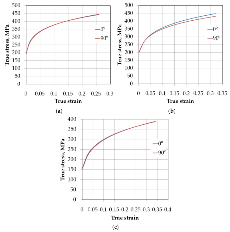
The sheets tested are commonly used in the automotive industry for the fabrication of drawpieces with complex shapes. The basic mechanical parameters of the sheet metals (Table 1) were determined in a uniaxial tensile test according to ISO 6892-1 [65] on specimens cut transverse to the rolling direction (90°) and along the rolling direction (0°). The values of the work hardening parameters (strengthening coefficient K and strain hardening exponent n) were determined based on an approximation of the true stress–true strain relation (Figure 1) by the power law equation σp = K·εn, where σp is the true stress and ε is plastic strain.
Table 1.
Basic mechanical parameters of the sheets tested.
| Material | Orientation | Yield Stress Rp0.2, MPa | Ultimate Tensile Stress Rm, MPa |
Strengthening Coefficient K, MPa |
Strain Hardening Exponent n |
|---|---|---|---|---|---|
| DQ | 0° | 193 | 351 | 554 | 0.166 |
| 90° | 193 | 353 | 563 | 0.174 | |
| DDQ | 0° | 196 | 336 | 557 | 0.192 |
| 90° | 198 | 311 | 526 | 0.177 | |
| EDDQ | 0° | 151 | 282 | 494 | 0.221 |
| 90° | 153 | 287 | 487 | 0.211 |
Figure 1.
The true stress–true strain curves of the test sheets: (a) DQ, (b) DDQ and (c) EDDQ.
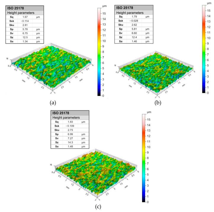
The measurement of the surface roughness parameters of the test sheets was carried out using a T8000RC profilometer in accordance with the requirements of the ISO 25178 standard [66]. The main standard 3D parameters and surface topographies determined by this measurement are listed in Figure 2. Sheet surfaces were sampled with an area of 3 mm × 3 mm.
Figure 2.
The surface topographies of the test sheets: (a) DQ, (b) DDQ and (c) EDDQ.
2.2. Experimental Setup
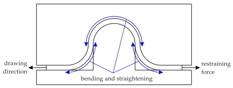
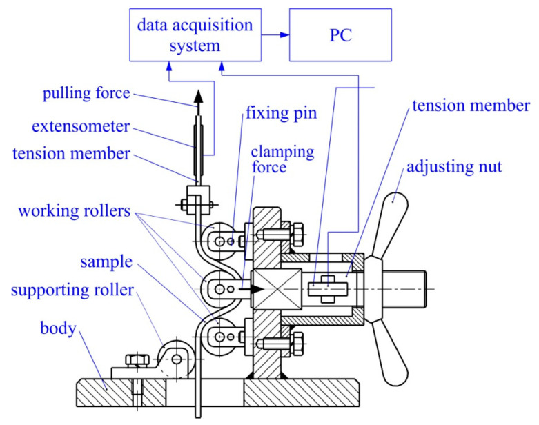
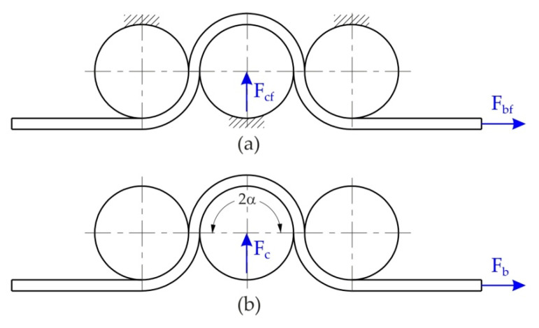
The drawbead test permitted the simulation of the bending and unbending in SMF and the measurement of the COF during the sliding of the sheet against a die. During the passage of the sheet metals through the drawbead, the sheet is bent and straightened three times (Figure 3). The idea behind the design of the proposed drawbead simulator (Figure 4) is the possibility of separating the frictional resistance of the sheet from the total resistance of the passage of the sheet metal through the drawbead and thus determining the value of the COF on the basis of the concept proposed by Nine [35].
Figure 3.
The bending and straightening of the sheet metal in the drawbead region.
Figure 4.
The drawbead simulator.
The tester consists of a body to which three working counter-samples and one guide counter-sample made of X165CrV12 cold-work tool steel were attached. The tester was mounted on the lower grip of a uniaxial tensile testing machine. The rotational motion of the working counter-samples was blocked by fixing pins. The value of the drawbead height was set by holding notes. The diameter of the counter-samples was 20 mm. During the tests, the pulling force and clamping force were measured using strain gauges. Measurement signals were transmitted to the 8-channel HBM amplifier, and then to a computer with QuantumX Assistant v1.1 R1 software, enabling cooperation with the amplifier and the recording of the clamping and pulling forces.
The friction test consisted of pulling the sheet strips in conditions involving either fixed or rotatable cylindrical counter-samples. During friction with the participation of fixed counter-samples, changes were registered in the pulling force Fbf and the clamping force Fcf. Similarly, under frictional conditions with freely movable rollers, the pulling force Fb and the clamping force Fc were measured (Figure 5). The friction test realised in the presence of fixed counter-samples represents the total resistance of the sheet metal passing through the drawbead.
Figure 5.
A conceptual diagram of the process for measuring force in the drawbead test in the presence of (a) fixed and (b) rotatable counter-samples.
The value of the COF was determined according to the relationship [35]:
| (1) |
where: Fb is the pulling force at the rotatable rollers, Fcf is clamping force with fixed rollers, Fbf is pulling force with fixed rollers, and 2α = π/2 confirms a full penetration of the middle counter-sample.
Samples in the form of strips of sheet 200 mm long and 20 mm wide were used as the test material. They were cut lengthways and transversely to the rolling direction of the sheet. One end of the sample was mounted on an upper grip of a uniaxial tensile testing machine. The pulling speed of the sample was 1 mm/s. Four sets of counter-samples were used with a surface roughness Ra equal to 0.32, 0.63, 1.25 and 2.5 μm in such a way as to ensure a wide range of variability in the Ra roughness parameter. Before starting the tests, the samples were cleaned with acetone. The tests were carried out under the conditions of dry friction and lubrication of the sheet surface with machine oil LAN46 and hydraulic oil LHL32. The basic physical properties of the oils based on the material cards provided by the producers are presented in Table 2.
Table 2.
The basic physical properties of oils.
| Oil | Kinematic Viscosity, mm2/s | Viscosity Index | Density kg/m3 |
|---|---|---|---|
| LAN46 | 43.9 | 94 | 875 |
| LHL32 | 32 | 95 | 875 |
2.3. Artificial Neural Networks
Rumelhart, McClelland and Hinton introduced the multilayer perceptron (MLP) notion in 1986, after Werbos’ 1974 proposal [67]. Network topology is the layout of network elements and their inputs, outputs and connections. The structure of an ANN can be described by the number of input and output layers, transfer functions between these levels and neurons in each layer [68]. A hidden layer separates the ANN’s input and output layers. Each network layer has many neurons. The number of input variables and output neurons is the same. Based on the transfer or activation function, these layers’ neurons transfer weight backward and forward [69]. Backpropagation learning to model an ANN with a multilayer perceptron (MLP) structure was used in this study. The multilayer perceptron is defined in Equation (2):
| (2) |
where is the output and is the input, are the weights and is the bias [70].
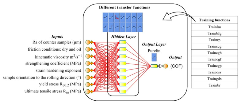
COF values were predicted using MLP structures in MATLAB R2022a [71]. Figure 6 shows that the network structure has one hidden layer with 10 neurons linking to the input and output layers for this investigation. Target datasets utilizing real measured data from three material investigations were adopted. The whole data was accumulated from three types of deep-drawing steel sheets (DQ, DDQ, and EDDQ). Eight neurons were inputs: Ra of the counter-samples (μm), friction conditions: dry and oil, kinematic viscosity m2·s−1, sample orientation to the rolling direction (°), yield stress Rp0.2 (MPa), ultimate tensile stress Rm (MPa), strengthening coefficient (MPa), strain hardening exponent, and COF values were outputs. It is worth to mention that two oils were chosen: machine oil LAN46 and hydraulic oil LHL32. This study employed 1000 epochs, 0.01 and 0.0001 as training parameters.
Figure 6.
Multilayer perceptron structures.
In order to find the optimal model and structure, different training and transfer functions, listed in Table 3 and Table 4, were trained. The main training parameters were a learning rate of 0.01, a performance target of 0.001 and 1000 epochs. While a neural network is functional and has many potential uses, it has certain limitations. Under or overfitting is one problems that can arise. Overfitting occurs when a network produces a more significant error for a new dataset than for the one it was trained on. Underfitting occurs when the model is too simplistic for training on the chosen dataset. A trained network can remember the acquired knowledge but has not been taught to generalize to unfit data. Figure 7 displays numerous instances of regression data fitting. Since increasing the size of an ensemble set does not reliably improve the accuracy but can decrease the generalizability [72], boosting algorithms are typically accompanied by regularization approaches to prevent overfitting [73]. Using an extensive network to provide a good fit, training multiple networks to ensure good generalization, averaging the outputs of the trained numerous neural networks, randomly separating data and tuning the complexity of a network through regularization [74] are just a few examples of how to improve and handle network generalization. In the MLP network created for the purpose of prediction in this study, generalization was improved by the so-called early stopping method. Early stopping to improve generalization was used in this study’s MLP network for prediction. All supervised network generation functions, including backpropagation networks, use early stopping by default [2]. If data overfitting restarts during network training, validation subset errors will increase. If the validation error rises over the minimum at a significantly different iteration number and exceeds the test subset error, the training stops and network weights and biases return to the minimal validation error [71].
Table 3.
Details of training functions used in multilayer perceptron.
| Algorithm | Acronym | Long Term |
|---|---|---|
| Trainlm | LM | Levenberg–Marquardt |
| Trainbfg | BFG | BFGS Quasi-Newton |
| Trainrp | RP | Resilient Backpropagation |
| Trainscg | SCG | Scaled Conjugate Gradient |
| Traincgb | CGB | Conjugate Gradient with Powell/Beale Restarts |
| Traincgf | CGF | Fletcher–Powell Conjugate Gradient |
| Traincgp | CGP | Polak–Ribiére Conjugate Gradient |
| Trainoss | OSS | One Step Secant |
| Traingdx | GDX | Variable Learning Rate Backpropagation |
| Trainbr | BRB | Bayesian Regularization Backpropagation |
Table 4.
Details of transfer functions used in multilayer perceptron.
| Acronym | Long Term | Equations |
|---|---|---|
| Elliotsig | Elliot sigmoid | f(x) = elliotsig(x) = (x)/1+|x| |
| Hardlim | Positive hard limit |
f(x) = hardlim(x) = 1, if x ≥ 0;
=0, otherwise. |
| Hardlims | Symmetric hard limit |
f(x) = hardlim(x) = 1, if x ≥ 0;
=−1, otherwise. |
| Logsig | Logarithmic sigmoid | f(x) = logsig(x) = 1/(1 + exp(−x)) |
| Netinv | Inverse | f(x) = netinv (x) = 1/x |
| Poslin | Positive linear |
f(x) = poslin(x) = x, if x
≥
0;
=0, if x ≤ 0. |
| Purelin | Linear | f(x) = purelin(x) = x |
| Radbas | Radial basis | f(x) = radbas(x) = exp (−x2) |
| Radbasn | Radial basis normalized | f(x) = radbasn(x) = exp (−x2)/sum(exp(−x2)) |
| Satlin | Positive saturating linear |
f(x) = satlin(x) = 0, if x ≤ 0;
=x, if 0 ≤ x ≤ 1; =1, if 1 ≤ x. |
| Satlins | Symmetric saturating linear |
f(x) = satlins(x) = −1, if x ≤ −1;
=x, if −1 ≤ x ≤ 1; =1, if 1 ≤ x. |
| Softmax | Soft max | f(x) = softmax(x) = exp(x)/sum(exp(x)) |
| Tansig | Symmetric sigmoid | f(x) = tansig(x) = 2/(1+exp (−2 ∗ x)) − 1 |
| Tribas | Triangular basis |
f(x) = tribas(x) = 1 − abs(x), if −1 ≤ x ≤ 1;
=0, otherwise. |
Where x is the weighted sum of w, i, b, and y of Equation (2).
Figure 7.
Different types of data fitting.
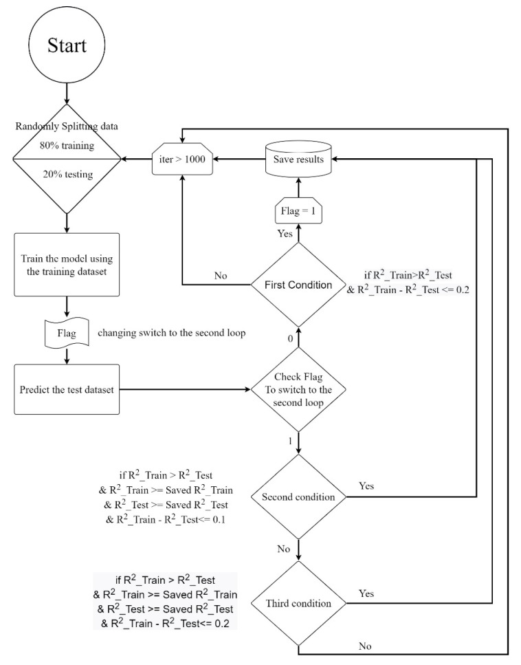
In neural networks, dataset training uses optimization to tune and find network weights for a good prediction map. Optimization algorithms are called training functions. Training the network to identify a given input and map it to an output is the training function. Performance goals, trained datasets, weights and biases affect the training function. Selecting a suitable training function for the network is one challenge in making good, rapid and accurate predictions. The transfer function computes each layer’s output by adopting cumulative weights entering the layer. Transfer functions depend on network structure and are difficult to set. This study used fifteen transfer functions individually to increase the prediction accuracy. The output layer’s linear (Purelin) transfer function was chosen in all circumstances. Figure 8 depicts the generated model’s training flowchart as well as the testing procedure utilizing test data. During the running process, two major conditions create decisions. The first loop preserves the model and all variables in the first condition with low conditional limits. After the first condition is met, the second loop is initiated and terminated by a stricter condition. The second loop starts the training and compares them to the variables saved from the prior training and repeats this process until 1000 iterations are completed. The third loop increases the conditional limit in case of not fulfilling the condition requirements in the second loop. To save the results, shared step loops are provided.
Figure 8.
Flowchart of the MLP model that was developed.
Collected data must be divided into training, validation and testing sets. The dataset’s training and testing subsets affect prediction accuracy and training performance [75]. Benchmark performance suffers from inappropriate subsets. Shahin [76] said the dataset’s splitting ratio has no apparent relationship, whereas Zhang et al. [75] reported it as one of the primary issues. However, there is no standard setting for the mentioned issue. Most researchers separate the datasets into lines with varying subgroup ratios based on their surveys. 90% vs. 10%, 80% vs. 20%, or 70% vs. 30% are the most common training and testing ratios. In this paper’s training run, the optimal prediction was achieved by dividing the actual data (72 samples) into training and testing datasets at 80% and 20%, respectively. The dataset consisted of 72 rows from experimental components used for training and testing.
3. Results and Discussion
3.1. Experimental Results
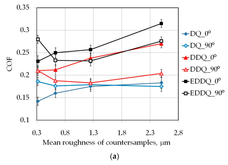
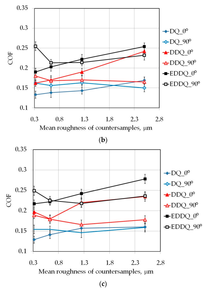
In general, the value of the coefficient of friction increased with increasing surface roughness of the counter-samples (Figure 9). It is clear that in dry friction conditions and for the surface roughness of counter-samples Ra = 0.32 μm (Figure 9a), samples cut perpendicularly to the rolling direction of the sheet showed a greater value for the coefficient of friction than samples cut along the sheet rolling direction. With a further increase in the roughness of the counter-samples, the relationship was reversed. This is due to the large contact surface that occurs when friction is made between surfaces with low roughness. Under these conditions, there is a strong mechanical interaction of the surface asperities, which in the case of sheet metal are displaced as a result of the texture created in the cold-rolling process of the sheet metal. A similar situation occurred during friction tests under lubrication with LAN46 machine oil (Figure 9b) and LHL32 hydraulic oil (Figure 9c). The influence of roughness on the effectiveness of lubrication is most important during the friction of bodies with low roughness. Then, it is possible to form valleys creating oil pockets on the friction face in which the hydrostatic pressure of the oil closed in the valleys creates a so-called “lubricant cushion” limiting the metallic contact of the friction faces. As the roughness of the counter-samples increases, the area of contact surface decreases, but a most intensive interaction occurs between the tool roughness asperities and the relatively soft material of the sample.
Figure 9.
Effect of mean roughness of counter-samples on the COF determined in (a) dry friction conditions and lubrication with (b) LAN46 machine oil and (c) LHL32 hydraulic oil.
To investigate the effect of lubricant on the friction coefficient, let us enter the parameter effectiveness of lubrication (EOL) determined according to the formula:
| (3) |
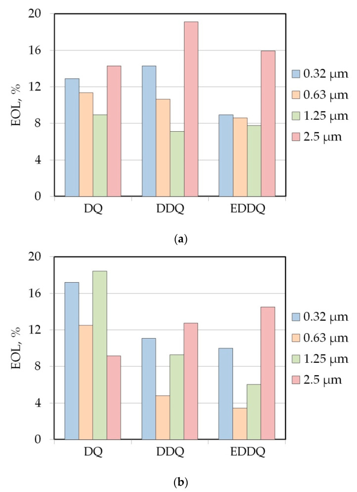
In the case of LAN46 machine oil (Figure 10a), the effectiveness of lubrication decreased in the range of roughness of counter-samples between Ra = 0.32–1.25 μm. It was for the roughness of counter-samples of 2.5 mm that the lubricant decreased the friction coefficient to the greatest extent (14.3–19.1%). The increase in EOL value can be explained by larger spaces that lie between surface asperities of the counter-samples with the parameter Ra = 2.5 μm. In terms of the roughness of the Ra = 0.32–1.25 μm counter-samples, the dominant friction mechanism was mechanical surface flattening and roughening. The influence of the lubricant on COF was less significant under these conditions. The change in viscosity of the lubricant used, i.e., LHL32, significantly changed the influence of the roughness of the counter-samples on the value of the EOL parameter (Figure 10b).
Figure 10.
Effectiveness of lubrication for samples cut perpendicular to the sheet rolling direction tested with the presence of (a) LAN46 machine oil and (b) LHL32 hydraulic oil.
With increasing drawing quality of the sheet metal, the value of the EOL decreased but only in the range of surface roughness of counter-samples between Ra = 0.32–1.25 μm. In the case of the counter-samples with surface roughness Ra = 2.5 μm, the situation was reversed. Similarly, to lubrication with LAN46 machine oil, the highest lubrication efficiency was observed for counter-samples with a surface roughness Ra = 2.5 μm but only for DDQ and EDDQ materials. Under these conditions, the efficiency of lowering of the friction coefficient by LHL32 hydraulic lubricant (Figure 10b) was generally lower than that of the LAN46 hydraulic oil (Figure 10a). Interpretation of the differences in the efficiency of lubricating oils for the DQ steel sheet was not unambiguous due to many phenomena and parameters that synergistically affect the value of the COF. Therefore, the next section of this article presents the use of artificial neural networks to analyse the experimental results of the DBS test.
3.2. Results of ANN Modelling
Using the right validation metric to evaluate a predictive model is crucial. This study compared and validated several structures, training and transferring methods for measuring the agreement between actual and predicted values. Choosing the right validation metric is vital and challenging to evaluate outcomes and reduce errors. All structures and models trained and tested in this work were compared using good metrics to assess test performance. Training and test errors must be distinguished. Test errors are determined using a stored entire dataset unknown to the model, while training errors are derived using the same data. The training dataset R2 value reveals variation within the trained samples through the model, while the testing dataset R2 value indicates the model’s predictive quality.
MLP’s best outcomes from using several models with varied training and transfer functions have been summarized, with more thorough evaluations shown in Appendix A (Table A1). When material B, SB and SSB were employed, Table 5 shows the best values of numerous validation metrics used to evaluate MLP training and transfer functions performance. Table 5 contains the following statistical parameters: ME—mean error, MAE—mean absolute error, MSE—mean square error, RMSE—root mean square error, MRE—mean relative error, SD—standard deviation, SEM—standard error mean. Models and structures are assessed using R2 and adj. R2.
Table 5.
Validation metrics of the best multilayer perceptron (MLP) models for predicting COF.
| Training Function | Bayesian Regularization Backpropagation (BRB)—Trainbr | ||
|---|---|---|---|
| Transfer Function | Radial Basis Normalized—Radbasn | ||
| Validation Metric | Training | Testing | Average (Training and Testing) |
| ME | 0.0005 | −0.0014 | 0.0001 |
| MAE | 0.0081 | 0.0086 | 0.0082 |
| MSE | 0.0001 | 0.0001 | 0.0001 |
| RMSE | 0.0108 | 0.0118 | 0.0110 |
| MRE | 0.0404 | 0.0415 | 0.0406 |
| SD | 0.0109 | 0.0122 | 0.0111 |
| SEM | 0.0014 | 0.0033 | 0.0013 |
| R2 | 0.9318 | 0.9180 | 0.9293 |
| adj. R2 | 0.9219 | 0.9160 | 0.9195 |
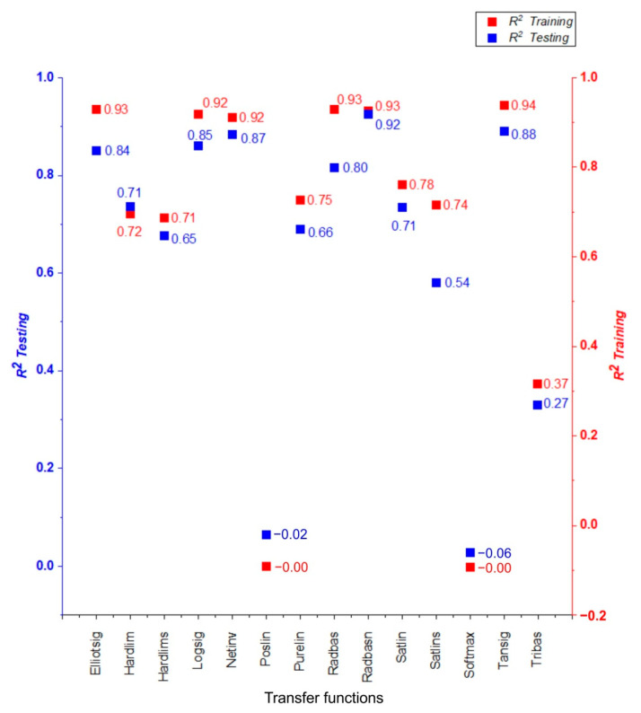
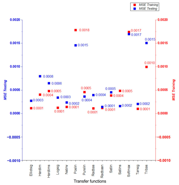
When the R2 of the testing was compared to all algorithms, it was discovered that the constructed MLP model performed the best in terms of COF prediction. Using Bayesian regularization backpropagation (BRB)—Trainbr as a training function and radial basis normalized—Radbasn as a transfer function, the greatest performance in predicting the COF was obtained. See Table A1 in the Appendix A for a summary of the results of all training and transfer functions. Figure 11 and Figure 12 depict R2 and MSE, respectively for each of the transfer functions predicted by the ANN using the Trainbr training function.
Figure 11.
Evaluation of different transfer functions using Bayesian regularization backpropagation (BRB)—Trainbr training function by R2 values.
Figure 12.
Evaluation of different transfer functions using Bayesian regularization backpropagation (BRB)—Trainbr training function by MSE values.
Instead of constructing, executing and evaluating a new ANN model each time, analytical equations were extracted from the best model to predict COF easily, practically and rapidly. Thus, the Radbasn transfer function is represented by Equation (4). Equation (5) provides a prediction of COF before the weights and biases were included. As a result, Equation (6) demands consistent weights and biases from the best-performing ANN network to predict COF analytically. Equation (7) calculates the COF directly and only by adding the values of the process parameters. The retrieved ANN network weights and biases served as one set of input weights (IW) and layer weights (LW). The IW is between the inputs and the hidden layer, the LW is between the hidden and output layers, and b1 and b2 are each layer’s biases. The biases b1, b2, IW and LW of the best-trained ANN model are shown in Table A2 in Appendix A.
| (4) |
| (5) |
| (6) |
| (7) |
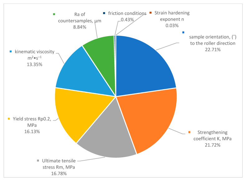
Feature, variable or relative importance is the examination of the input variables on the outputs. However, this analysis shows how each feature’s value affects the model’s prediction averages, indicating its relative importance. Substituting the input variables with high relative importance (RI) values affects results more than variables with lower RI values [68,77,78]. Garson [79], most squares [80], and connection weights [81] calculate the feature importance. Various research has calculated and assessed variable impacts using feature importance [78,82,83,84,85,86,87,88]. Figure 13 shows the relative importance and weight analysis of several important factors that affect COF. There are different ways to determine how the input variables affect the output, which is the COF, based on weights and biases. However, the Garson method was adopted in this study. The calculation shows that changes in the sample orientation (°) to the roller direction and strengthening coefficient K (MPa) significantly affect COF. Ultimate tensile stress Rm (MPa) and yield stress Rp0.2 (MPa) came in second concerning COF. Friction conditions and strain hardening exponent had a minor effect. It is possible that the relative importance regarding the friction conditions is not reasonable because the data has been categorically encoded and binarized using one hot encoding. All the actual and predicted COF values for the training and testing datasets are listed in the Appendix A (Table A3).
Figure 13.
The relative importance and weight analysis of several important factors that affect COF.
4. Conclusions
This article presented the results of ANN analysis of the friction behaviour of drawing quality steel sheets in drawbead profiles during sheet metal forming. The experimental results were used to train artificial neural networks. The following conclusions can be drawn from the results presented in this article:
A trend of increasing the COF with increasing the mean surface roughness of the counter-samples was observed for all friction conditions analysed.
As the surface roughness of the counter-samples increased, the area of contact surface decreased; however, the resulting coefficient of friction is a result of the coexistence of the following mechanisms: surface flattening and roughening, and lubrication.
Favourable lubrication conditions occur with low roughness of a soft friction pair (workpiece) compared to the surface properties of the counter-samples.
The MLP algorithm successfully predicted the coefficient of friction with R2 values from 0.9318 for the training dataset and 0.9180 for the testing dataset, with an average R2 value of 0.9293 for both the training and testing datasets.
When it came to predict the coefficient of friction accurately, the Bayesian regularization backpropagation (BRB)—Trainbr training method fared the best. The radial basis normalized—Radbasn transfer function provided the best prediction of the COF.
The relative significance (RI) methods given that sample orientation to the sheet rolling direction and strengthening coefficient significantly affected COF. The ultimate tensile and yield stress are tied in second place in terms of influences on COF. There is only a slight influence from the friction conditions and the strain hardening exponent.
Acknowledgments
The artificial intelligence-related research reported in this paper and carried out at the BME by the second author was partially supported through the National Laboratory of Artificial Intelligence funded by the NRDIO under the auspices of the Ministry for Innovation and Technology.
Appendix A
Table A1.
The validation metrics of all training and transfer functions of the multilayer perceptron (MLP) models for predicting COF.
| Training Function | Levenberg–Marquardt (LM)—Trainlm | ||||||||||||||
|---|---|---|---|---|---|---|---|---|---|---|---|---|---|---|---|
| Transfer Function | Elliotsig | Hardlim | Hardlims | Logsig | Netinv | Poslin | Purelin | Radbas | Radbasn | Satlin | Satlins | Softmax | Tansig | Tribas | |
| Training | R2 | 0.8730 | 0.6622 | 0.7774 | 0.3718 | 0.9315 | 0.8189 | 0.8414 | 0.2051 | 0.8735 | 0.8779 | 0.8775 | −0.0008 | −0.0182 | 0.0319 |
| MSE | 0.0002 | 0.0006 | 0.0004 | 0.0010 | 0.0001 | 0.0003 | 0.0002 | 0.0014 | 0.0002 | 0.0002 | 0.0002 | 0.0016 | 0.0017 | 0.0016 | |
| Testing | R2 | 0.7875 | 0.4633 | 0.6164 | 0.2741 | 0.8913 | 0.7777 | 0.8049 | 0.0418 | 0.7690 | 0.8459 | 0.8527 | −0.0044 | −0.1474 | 0.0301 |
| MSE | 0.0004 | 0.0007 | 0.0005 | 0.0016 | 0.0002 | 0.0005 | 0.0006 | 0.0015 | 0.0004 | 0.0004 | 0.0002 | 0.0021 | 0.0022 | 0.0019 | |
| Training function | BFGS Quasi-Newton (BFG)—Trainbfg | ||||||||||||||
| Training | R2 | 0.5293 | 0.6093 | 0.6994 | −0.0006 | 0.8169 | −0.0045 | 0.0896 | 0.0000 | −0.0047 | −0.0007 | −0.0002 | 0.0103 | −0.0043 | −0.8322 |
| MSE | 0.0008 | 0.0007 | 0.0006 | 0.0019 | 0.0003 | 0.0018 | 0.0014 | 0.0018 | 0.0019 | 0.0017 | 0.0018 | 0.0014 | 0.0017 | 0.0032 | |
| Testing | R2 | 0.3481 | 0.5398 | 0.5154 | −0.0518 | 0.6747 | −0.0326 | −0.0501 | −0.0621 | −0.0078 | −0.1610 | −0.1712 | −0.0543 | −0.0266 | −0.9412 |
| MSE | 0.0009 | 0.0006 | 0.0004 | 0.0009 | 0.0004 | 0.0014 | 0.0026 | 0.0014 | 0.0010 | 0.0017 | 0.0016 | 0.0032 | 0.0021 | 0.0031 | |
| Training function | Resilient Backpropagation (RP)—Trainrp | ||||||||||||||
| Training | R2 | 0.8856 | 0.5644 | 0.7729 | 0.8950 | 0.8701 | −0.2627 | 0.5016 | −0.0036 | −0.0307 | −0.0206 | −0.0076 | −0.5355 | 0.0000 | −0.6498 |
| MSE | 0.0002 | 0.0007 | 0.0004 | 0.0002 | 0.0002 | 0.0022 | 0.0009 | 0.0016 | 0.0017 | 0.0015 | 0.0017 | 0.0029 | 0.0018 | 0.0031 | |
| Testing | R2 | 0.7544 | 0.4247 | 0.7373 | 0.8830 | 0.6753 | −0.3073 | 0.4009 | −0.0046 | −0.2294 | −0.1607 | −0.0947 | −0.5593 | −0.0197 | −0.7014 |
| MSE | 0.0003 | 0.0010 | 0.0006 | 0.0002 | 0.0008 | 0.0019 | 0.0007 | 0.0022 | 0.0022 | 0.0032 | 0.0019 | 0.0013 | 0.0012 | 0.0017 | |
| Training function | Scaled Conjugate Gradient (SCG)—Trainscg | ||||||||||||||
| Training | R2 | 0.8965 | 0.7040 | 0.7380 | 0.9293 | 0.7203 | −2.8003 | 0.6393 | 0.0589 | 0.4909 | −0.0007 | 0.0412 | −0.0009 | 0.5936 | −4.9884 |
| MSE | 0.0002 | 0.0005 | 0.0005 | 0.0001 | 0.0005 | 0.0062 | 0.0006 | 0.0016 | 0.0007 | 0.0016 | 0.0017 | 0.0018 | 0.0007 | 0.0100 | |
| Testing | R2 | 0.7557 | 0.5815 | 0.5412 | 0.9235 | 0.6609 | −2.9296 | 0.6249 | −0.0775 | 0.4900 | −0.0302 | −0.1379 | −0.0308 | 0.5858 | −5.0740 |
| MSE | 0.0006 | 0.0006 | 0.0008 | 0.0002 | 0.0006 | 0.0077 | 0.0006 | 0.0019 | 0.0014 | 0.0021 | 0.0018 | 0.0013 | 0.0006 | 0.0101 | |
| Training function | Conjugate Gradient with Powell/Beale Restarts (CGB)—Traincgb | ||||||||||||||
| Training | R2 | 0.9111 | 0.6653 | 0.7823 | 0.8965 | −0.0214 | 0.5384 | 0.6662 | −0.0001 | −0.0059 | 0.7371 | −0.0005 | −0.0261 | 0.6954 | 0.0000 |
| MSE | 0.0002 | 0.0006 | 0.0004 | 0.0002 | 0.0018 | 0.0008 | 0.0006 | 0.0016 | 0.0015 | 0.0004 | 0.0018 | 0.0019 | 0.0005 | 0.0017 | |
| Testing | R2 | 0.8293 | 0.5424 | 0.6019 | 0.7815 | −0.0428 | 0.4136 | 0.4838 | −0.0602 | −0.0497 | 0.5875 | −0.0083 | −0.0858 | 0.6272 | −0.0289 |
| MSE | 0.0003 | 0.0006 | 0.0006 | 0.0003 | 0.0016 | 0.0008 | 0.0009 | 0.0021 | 0.0026 | 0.0010 | 0.0016 | 0.0014 | 0.0007 | 0.0018 | |
| Training function | Fletcher–Powell Conjugate Gradient (CGF)—Traincgf | ||||||||||||||
| Training | R2 | 0.8495 | 0.5491 | 0.5807 | 0.5103 | 0.3220 | −1.6810 | 0.6662 | −0.0015 | −0.0002 | −0.0002 | −0.0031 | −0.0014 | −0.0020 | −0.0001 |
| MSE | 0.0003 | 0.0007 | 0.0007 | 0.0008 | 0.0012 | 0.0046 | 0.0006 | 0.0017 | 0.0018 | 0.0019 | 0.0018 | 0.0017 | 0.0019 | 0.0017 | |
| Testing | R2 | 0.7948 | 0.5297 | 0.5495 | 0.3660 | 0.1933 | −1.8698 | 0.4838 | −0.0412 | −0.0221 | −0.0142 | −0.0271 | −0.0056 | −0.0089 | −0.1788 |
| MSE | 0.0004 | 0.0010 | 0.0007 | 0.0013 | 0.0012 | 0.0048 | 0.0009 | 0.0017 | 0.0014 | 0.0011 | 0.0014 | 0.0018 | 0.0010 | 0.0018 | |
| Training function | Polak–Ribiére Conjugate Gradient (CGP)—Traincgp | ||||||||||||||
| Training | R2 | 0.5955 | 0.5645 | 0.7784 | 0.0086 | 0.3507 | −4.4318 | −77.6014 | −0.0010 | −0.0005 | −0.0016 | −0.0029 | 0.0000 | 0.4306 | −0.0003 |
| MSE | 0.0007 | 0.0007 | 0.0003 | 0.0017 | 0.0011 | 0.0099 | 0.1404 | 0.0018 | 0.0017 | 0.0014 | 0.0019 | 0.0019 | 0.0010 | 0.0014 | |
| Testing | R2 | 0.4401 | 0.4315 | 0.7301 | −0.0084 | 0.2503 | −4.5725 | −77.7437 | −0.0942 | −0.0848 | −0.0720 | −0.0625 | −0.1148 | 0.2817 | −0.0188 |
| MSE | 0.0009 | 0.0009 | 0.0006 | 0.0016 | 0.0014 | 0.0073 | 0.0937 | 0.0013 | 0.0020 | 0.0029 | 0.0010 | 0.0010 | 0.0011 | 0.0029 | |
| Training function | One Step Secant (OSS)—Trainoss | ||||||||||||||
| Training | R2 | 0.5604 | −0.0399 | −0.1893 | −0.0036 | 0.5851 | 0.2590 | 0.2152 | −0.3388 | −0.0002 | −0.0002 | −0.0003 | 0.0000 | −0.0001 | 0.0000 |
| MSE | 0.0007 | 0.0017 | 0.0020 | 0.0017 | 0.0008 | 0.0013 | 0.0013 | 0.0024 | 0.0017 | 0.0019 | 0.0020 | 0.0017 | 0.0019 | 0.0017 | |
| Testing | R2 | 0.5409 | −0.1051 | −0.2987 | −0.0484 | 0.4091 | 0.2245 | 0.1251 | −0.3659 | −0.0188 | −0.0142 | −0.0160 | −0.0117 | −0.0156 | −0.0176 |
| MSE | 0.0006 | 0.0021 | 0.0022 | 0.0016 | 0.0008 | 0.0010 | 0.0016 | 0.0021 | 0.0016 | 0.0011 | 0.0007 | 0.0018 | 0.0010 | 0.0018 | |
| Training function | Variable Learning Rate Backpropagation (GDX)—Traingdx | ||||||||||||||
| Training | R2 | −0.0005 | 0.7337 | 0.6988 | −1.4754 | 0.3543 | −0.0001 | 0.6662 | −0.3164 | −0.0014 | −0.0011 | 0.4030 | 0.0000 | −0.0006 | −0.0022 |
| MSE | 0.0017 | 0.0005 | 0.0005 | 0.0046 | 0.0011 | 0.0015 | 0.0006 | 0.0023 | 0.0018 | 0.0017 | 0.0010 | 0.0017 | 0.0016 | 0.0015 | |
| Testing | R2 | −0.0009 | 0.6728 | 0.5573 | −1.6742 | 0.3401 | −0.1135 | 0.4838 | −0.4212 | −0.0509 | −0.0116 | 0.3546 | −0.0383 | −0.1115 | −0.0801 |
| MSE | 0.0017 | 0.0005 | 0.0008 | 0.0031 | 0.0011 | 0.0028 | 0.0009 | 0.0023 | 0.0013 | 0.0019 | 0.0013 | 0.0017 | 0.0024 | 0.0027 | |
| Training function | Bayesian Regularization Backpropagation (BRB)—Trainbr | ||||||||||||||
| Training | R2 | 0.9344 | 0.7203 | 0.7128 | 0.9242 | 0.9188 | −0.0011 | 0.7484 | 0.9340 | 0.9318 | 0.7811 | 0.7384 | −0.0024 | 0.9435 | 0.3717 |
| MSE | 0.0001 | 0.0004 | 0.0005 | 0.0001 | 0.0001 | 0.0018 | 0.0005 | 0.0001 | 0.0001 | 0.0004 | 0.0005 | 0.0017 | 0.0001 | 0.0010 | |
| Testing | R2 | 0.8360 | 0.7120 | 0.6457 | 0.8475 | 0.8728 | −0.0208 | 0.6610 | 0.7986 | 0.9180 | 0.7102 | 0.5419 | −0.0619 | 0.8796 | 0.2674 |
| MSE | 0.0003 | 0.0008 | 0.0006 | 0.0003 | 0.0002 | 0.0015 | 0.0004 | 0.0004 | 0.0001 | 0.0005 | 0.0002 | 0.0017 | 0.0002 | 0.0015 | |
Table A2.
The weights and biases of the best MLP model for predicting COF (Trainbr with Radbasn).
| b 1 | b 2 | IW | LW | |||||||
|---|---|---|---|---|---|---|---|---|---|---|
| −0.000013 | 0.154802302 | 0.000302 | 0.000664 | 0.000043 | 0.002863 | −0.002295 | −0.004105 | −0.006618 | −0.000002 | 0.014177 |
| 0.000054 | 0.000674 | −0.056316 | 0.000430 | 0.005001 | −0.003263 | −0.006876 | 0.013543 | 0.000031 | 0.004673 | |
| −0.000036 | 0.000158 | 0.000150 | −0.000018 | −0.001888 | 0.008779 | 0.008167 | 0.002309 | −0.000019 | −0.000515 | |
| 0.000032 | −0.000338 | −0.004919 | 0.000113 | 0.005465 | 0.000295 | 0.004110 | 0.010179 | 0.000011 | 0.003907 | |
| −0.000016 | 0.000167 | −0.001404 | −0.000017 | −0.000267 | −0.002455 | −0.004589 | −0.007722 | −0.000003 | 0.000085 | |
| −0.000073 | 0.000563 | −0.013884 | −0.000797 | −0.032309 | 0.009952 | 0.007066 | 0.003993 | −0.000026 | 0.018840 | |
| 0.000031 | −0.060694 | 0.058730 | −0.001589 | −0.004534 | −0.014893 | 0.003317 | −0.004841 | 0.000006 | −0.035940 | |
| 0.000013 | 0.000182 | 0.003415 | 0.000004 | 0.000139 | 0.002099 | 0.003924 | 0.007039 | 0.000003 | −0.002575 | |
| 0.000000 | −0.044608 | −0.040035 | 0.000055 | 0.007430 | 0.008765 | 0.010053 | −0.001046 | −0.000037 | 0.145881 | |
| −0.000022 | −0.000054 | −0.004141 | 0.000174 | 0.006514 | 0.012974 | 0.002716 | 0.004050 | −0.000017 | 0.006270 | |
Table A3.
All the actual and predicted values of COF (trained and tested sets).
| Training Dataset | Testing Dataset | ||||
|---|---|---|---|---|---|
| Actual | Predicted | Actual | Predicted | ||
| 1 | 0.183 | 0.188 | 1 | 0.236 | 0.235 |
| 2 | 0.188 | 0.198 | 2 | 0.156 | 0.157 |
| 3 | 0.257 | 0.265 | 3 | 0.178 | 0.179 |
| 4 | 0.217 | 0.211 | 4 | 0.175 | 0.178 |
| 5 | 0.162 | 0.157 | 5 | 0.233 | 0.251 |
| 6 | 0.183 | 0.197 | 6 | 0.133 | 0.137 |
| 7 | 0.168 | 0.172 | 7 | 0.203 | 0.204 |
| 8 | 0.17 | 0.172 | 8 | 0.27 | 0.267 |
| 9 | 0.162 | 0.166 | 9 | 0.19 | 0.194 |
| 10 | 0.278 | 0.275 | 10 | 0.18 | 0.171 |
| 11 | 0.16 | 0.168 | 11 | 0.28 | 0.252 |
| 12 | 0.154 | 0.161 | 12 | 0.166 | 0.178 |
| 13 | 0.22 | 0.207 | 13 | 0.16 | 0.153 |
| 14 | 0.165 | 0.173 | 14 | 0.25 | 0.250 |
| 15 | 0.186 | 0.177 | 15 | 0.197 | 0.176 |
| 16 | 0.235 | 0.244 | 16 | 0.179 | 0.178 |
| 17 | 0.157 | 0.149 | 17 | 0.212 | 0.218 |
| 18 | 0.222 | 0.223 | 18 | 0.236 | 0.235 |
| 19 | 0.231 | 0.240 | |||
| 20 | 0.142 | 0.148 | |||
| 21 | 0.222 | 0.223 | |||
| 22 | 0.232 | 0.250 | |||
| 23 | 0.129 | 0.139 | |||
| 24 | 0.238 | 0.238 | |||
| 25 | 0.214 | 0.230 | |||
| 26 | 0.225 | 0.237 | |||
| 27 | 0.19 | 0.195 | |||
| 28 | 0.213 | 0.230 | |||
| 29 | 0.265 | 0.231 | |||
| 30 | 0.249 | 0.237 | |||
| 31 | 0.146 | 0.162 | |||
| 32 | 0.189 | 0.178 | |||
| 33 | 0.179 | 0.178 | |||
| 34 | 0.159 | 0.163 | |||
| 35 | 0.175 | 0.163 | |||
| 36 | 0.232 | 0.229 | |||
| 37 | 0.169 | 0.162 | |||
| 38 | 0.21 | 0.198 | |||
| 39 | 0.176 | 0.177 | |||
| 40 | 0.18 | 0.186 | |||
| 41 | 0.204 | 0.197 | |||
| 42 | 0.138 | 0.140 | |||
| 43 | 0.315 | 0.285 | |||
| 44 | 0.254 | 0.255 | |||
| 45 | 0.154 | 0.161 | |||
| 46 | 0.218 | 0.236 | |||
| 47 | 0.242 | 0.244 | |||
| 48 | 0.141 | 0.142 | |||
| 49 | 0.276 | 0.248 | |||
| 50 | 0.17 | 0.175 | |||
| 51 | 0.21 | 0.207 | |||
| 52 | 0.143 | 0.146 | |||
| 53 | 0.15 | 0.158 | |||
| 54 | 0.242 | 0.233 | |||
| 55 | 0.163 | 0.157 | |||
| 56 | 0.236 | 0.235 | |||
Author Contributions
Conceptualization, T.T.; methodology, T.T. and S.M.N.; investigation, T.T. and S.M.N.; data curation, T.T. and S.M.N.; writing—original draft preparation, T.T. and S.M.N.; writing—review and editing, T.T. and S.M.N. All authors have read and agreed to the published version of the manuscript.
Institutional Review Board Statement
Not applicable.
Informed Consent Statement
Not applicable.
Data Availability Statement
Data are contained within the article.
Conflicts of Interest
The authors declare no conflict of interest.
Funding Statement
This research received no external funding.
Footnotes
Publisher’s Note: MDPI stays neutral with regard to jurisdictional claims in published maps and institutional affiliations.
References
- 1.Najm S.M., Paniti I. Study on Effecting Parameters of Flat and Hemispherical end Tools in SPIF of Aluminium Foils. Tehnički Vjesnik. 2020;27:1844–1849. doi: 10.17559/TV-20190513181910. [DOI] [Google Scholar]
- 2.Najm S.M., Paniti I. Investigation and machine learning-based prediction of parametric effects of single point incremental forming on pillow effect and wall profile of AlMn1Mg1 aluminum alloy sheets. J. Intell. Manuf. 2022 doi: 10.1007/s10845-022-02026-8. [DOI] [Google Scholar]
- 3.Milutinović M., Lendjel R., Baloš S., Zlatanović D.L., Sevšek L., Pepelnjak T. Characterisation of geometrical and physical properties of a stainless steel denture framework manufactured by single-point incremental forming. J. Mater. Res. Technol. 2021;10:605–623. doi: 10.1016/j.jmrt.2020.12.014. [DOI] [Google Scholar]
- 4.Xia J., Zhao J., Dou S., Shen X. A Novel Method for Friction Coefficient Calculation in Metal Sheet Forming of Axis-Symmetric Deep Drawing Parts. Symmetry. 2022;14:414. doi: 10.3390/sym14020414. [DOI] [Google Scholar]
- 5.Centeno G., Silva M.B. Tube and Sheet Metal Forming Processes and Applications. Metals. 2022;12:553. doi: 10.3390/met12040553. [DOI] [Google Scholar]
- 6.Duarte E.N., Oliveira S.A.G., Weyler R., Nemati L. A hybrid approach for estimating the drawbead restraining force in sheet metal forming. J. Braz. Soc. Mech. Eng. 2010;32:282–291. doi: 10.1590/S1678-58782010000300012. [DOI] [Google Scholar]
- 7.Dou S., Xia J. Analysis of Sheet Metal Forming (Stamping Process): A Study of the Variable Friction Coefficient on 5052 Aluminum Alloy. Metals. 2019;9:853. doi: 10.3390/met9080853. [DOI] [Google Scholar]
- 8.Folle L.F., Caetano dos Santos Silva B., Sousa de Carvalho M., Zamorano L.G.S., Coelho R.S. Evaluation of the Friction Coefficient for TRIP1000 Steel under Different Conditions of Lubrication, Contact Pressure, Sliding Speed and Working Temperature. Metals. 2022;12:1299. doi: 10.3390/met12081299. [DOI] [Google Scholar]
- 9.Shisode M., Hazrati J., Mishra T., de Rooij M., ten Horn C., van Beeck J., van der Boogaard T. Modeling boundary friction of coated sheets in sheet metal forming. Tribol. Int. 2021;153:106554. doi: 10.1016/j.triboint.2020.106554. [DOI] [Google Scholar]
- 10.Xu Z., Huang J., Mao M., Peng L., Lai X. An investigation on the friction in a micro sheet metal roll forming processes considering adhesion and ploughing. J. Mater. Proc. Technol. 2020;285:116790. doi: 10.1016/j.jmatprotec.2020.116790. [DOI] [Google Scholar]
- 11.Pepelnjak T., Kaftanoglu B. Finite element analysis of non-isothermal warm deep drawing of dual phase steel. Matec Web Conf. 2016;80:14003. doi: 10.1051/matecconf/20168014003. [DOI] [Google Scholar]
- 12.Trzepiecinski T., Lemu H.G. Recent Developments and Trends in the Friction Testing for Conventional Sheet Metal Forming and Incremental Sheet Forming. Metals. 2020;10:47. doi: 10.3390/met10010047. [DOI] [Google Scholar]
- 13.Bensaid K., Fredj N.B. Influence of Sliding Speed and Normal Loads on the Wear Resistance of Hardox 500 Steel Ground Surfaces. In: Kharrat M., Baccar M., Dammak F., editors. Advances in Mechanical Engineering, Materials and Mechanics, Proceedings of the ICAMEM 2019, Hammamet, Tunisia, 16–18 December 2019. Springer; Cham, Switzerland: 2021. pp. 84–90. Lecture Notes in Mechanical Engineering. [DOI] [Google Scholar]
- 14.Bensaid K., Dhiflaoui H., Bouzaiene H., Yahyaoui H., Fredj N.B. Effects of the cooling mode on the integrity and the multi-pass micro-scratching wear resistance of Hardox 500 ground surfaces. Int. J. Adv. Manuf. Technol. 2021;113:2865–2882. doi: 10.1007/s00170-021-06719-x. [DOI] [Google Scholar]
- 15.Luiz V.D., Amaral E.C., de Souza V.P., de Matos Rodrigues P.C. Influência da velocidade de estampagem e anisotropia no comportamento tribológico e fratura de uma chapa de aço AISI 430Nb. Materia. 2022;27:e20148196. doi: 10.1590/1517-7076-RMAT-2021-48196. [DOI] [Google Scholar]
- 16.Zabala A., de Argandoña E.S., Cañizares D., Llavori I., Otegi N., Mendiguren J. Numerical study of advanced friction modelling for sheet metal forming: Influence of the die local roughness. Tribol. Int. 2022;165:107259. doi: 10.1016/j.triboint.2021.107259. [DOI] [Google Scholar]
- 17.Trzepieciński T. Tribological Performance of Environmentally Friendly Bio-Degradable Lubricants Based on a Combination of Boric Acid and Bio-Based Oils. Materials. 2020;13:3892. doi: 10.3390/ma13173892. [DOI] [PMC free article] [PubMed] [Google Scholar]
- 18.Trzepieciński T. Polynomial Multiple Regression Analysis of the Lubrication Effectiveness of Deep Drawing Quality Steel Sheets by Eco-Friendly Vegetable Oils. Materials. 2022;15:1151. doi: 10.3390/ma15031151. [DOI] [PMC free article] [PubMed] [Google Scholar]
- 19.Szewczyk M., Szwajka K., Trzepieciński T. Frictional Characteristics of Deep-Drawing Quality Steel Sheets in the Flat Die Strip Drawing Test. Materials. 2022;15:5236. doi: 10.3390/ma15155236. [DOI] [PMC free article] [PubMed] [Google Scholar]
- 20.Luiz V.D., de Matos Rodrigues P.C. Design of a Tribo-Simulator for Investigation of the Tribological Behavior of Stainless-Steel Sheets Under Different Contact Conditions. Mater. Res. 2022;25:e20210220. doi: 10.1590/1980-5373-mr-2021-0220. [DOI] [Google Scholar]
- 21.Luiz V.D., de Matos Rodrigues P.C. Effect of the test conditions on tribological behavior of an Nb-stabilized AISI 430 stainless steel sheet. J. Braz. Soc. Mech. Sci. Eng. 2021;43:505. doi: 10.1007/s40430-021-03235-7. [DOI] [Google Scholar]
- 22.Samuel M. Influence of drawbead geometry on sheet metal forming. J. Mater. Process. Technol. 2002;122:94–103. doi: 10.1016/S0924-0136(01)01233-X. [DOI] [Google Scholar]
- 23.Smith L.M., Zhou Y.J., Zhou D.J., Wanintudal C. A new experimental test apparatus for binder draw bead simulations. J. Mat. Proc. Technol. 2009;209:4942–4948. doi: 10.1016/j.jmatprotec.2009.01.017. [DOI] [Google Scholar]
- 24.Lanzon J.M., Cadew-Hall M.J., Hodgson P.D. Characterising frictional behaviour in sheet metal forming. J. Mat. Proc. Technol. 1998;80–81:251–256. doi: 10.1016/S0924-0136(98)00110-1. [DOI] [Google Scholar]
- 25.Sanchez L.R. Characterisation of a measurement system for reproducible friction testing on a sheet metal under plane strain. Tribol. Int. 1999;32:575–586. doi: 10.1016/S0301-679X(99)00098-5. [DOI] [Google Scholar]
- 26.Figueiredo L., Ramalho A., Oliveira M.C., Menezes L.F. Experimental study of friction in sheet metal forming. Wear. 2011;271:1651–1657. doi: 10.1016/j.wear.2011.02.020. [DOI] [Google Scholar]
- 27.Schey J.A. Speed effects in drawbead simulation. J. Mater. Proc. Technol. 1996;57:146–154. doi: 10.1016/0924-0136(95)02061-6. [DOI] [Google Scholar]
- 28.Huh H., Song J.H., Kim S.H., Kim S.H. Effect of the Draw-bead and Blanking Holding Force on the Sheet Metal Forming Process. AIP Conf. Proc. 2004;712:2004. doi: 10.1063/1.1766619. [DOI] [Google Scholar]
- 29.Dahham A., Refa’t A., Jaber M. Finite Element Analysis of Draw Beads in Deep Drawing Processes. Al-Rafidain Eng. 2014;22:1–13. [Google Scholar]
- 30.Wu Y., Recklin V., Groche P. Strain Induced Surface Change in Sheet Metal Forming: Numerical Prediction, Influence on Friction and Tool Wear. J. Manuf. Mater. Process. 2021;5:29. doi: 10.3390/jmmp5020029. [DOI] [Google Scholar]
- 31.Bassoli E., Sola A., Denti L., Gatto A. Experimental approach to measure the restraining force in deep drawing by means of a versatile draw bead simulator. Mater. Manuf. Proc. 2019;34:1286–1295. doi: 10.1080/10426914.2019.1628267. [DOI] [Google Scholar]
- 32.Manjula N.K.B., Nanayakkara P., Hodgson P.D. Determination of Drawbead Contacts with Variable Bead Penetration. Comp. Method. Mater. Sci. 2006;6:188–194. [Google Scholar]
- 33.Jansson T., Andersson A., Nilsson L. Optimization of Draw-In for an Automotive Sheet Metal Part an Evaluation Using Surrogate Models and Response Surfaces. J. Mater. Process. Technol. 2005;159:426–434. doi: 10.1016/j.jmatprotec.2004.06.011. [DOI] [Google Scholar]
- 34.Stoughton T.B. Model of drawbead forces in sheet metal forming; Proceedings of the 15th Biennial Congress of IDDRG; Dearborn, MI, USA. 16–18 May 1988; pp. 205–215. [Google Scholar]
- 35.Nine H.D. Drawbead forces in sheet metal forming. In: Koistinen D.P., Wang N.M., editors. Mechanics of Sheet Metal Forming. Plenum Press; New York, NY, USA: 1978. pp. 179–211. [Google Scholar]
- 36.Nanayakkara N.K.B.M.P., Kelly G.L., Hodgson P.D. Determination of the coefficient of friction in partially penetrated draw beads. Steel GRIPS. 2004;2:667–682. [Google Scholar]
- 37.Cillaurren J., Galdos L., Sanchez M., Zabala A., de Argandoña E.S., Mendiguren J. Contact pressure and sliding velocity ranges in sheet metal forming simulations; Proceedings of the ESAFORM 2021, 24th International Conference on Material Forming; Liège, Belgique. 14–16 April 2021; [DOI] [Google Scholar]
- 38.Duarte E.N., Oliveira S.A.G. The influence of sheet thickness on drawbead restraining force in sheet metal forming; Proceedings of the 18th Congress of Mechanical Engineering; Ouro Preto, Brasil. 6–11 November 2005; pp. 1–6. [Google Scholar]
- 39.Billade B., Dahake S. Design and Analysis of Draw Bead Profile in Sheet Metal Forming Of Reinf-Rr End Upr-Lh/Rh for Safe Thinning. Int. J. Eng. Sci. Innov. 2018;7:1–10. [Google Scholar]
- 40.Chen J., Zheng T., Chen Q., Zhang J. Investigation on frictional characteristics and drawbead restraining force of steel with/without coating. AIP Conf. Proc. 2013;1567:922. doi: 10.1063/1.4850120. [DOI] [Google Scholar]
- 41.Weinmann K.J., Michler J.R., Rao V.D., Kashani A.R. Development of a Computer-Controlled Drawbead Simulator for Sheet Metal Forming. Ann. CIRP. 1994;43:257–261. doi: 10.1016/S0007-8506(07)62208-2. [DOI] [Google Scholar]
- 42.Paturi U.M.R., Palakurthy S.T., Reddy N.S. The Role of Machine Learning in Tribology: A Systematic Review. Arch. Computat. Methods. Eng. 2022 doi: 10.1007/s11831-022-09841-5. [DOI] [Google Scholar]
- 43.Rosenkranz A., Marian M., Profito F.J., Aragon N., Shah R. The Use of Artificial Intelligence in Tribology—A Perspective. Lubricants. 2021;9:2. doi: 10.3390/lubricants9010002. [DOI] [Google Scholar]
- 44.Yuvalı M., Yaman B., Tosun Ö. Classification Comparison of Machine Learning Algorithms Using Two Independent CAD Datasets. Mathematics. 2022;10:311. doi: 10.3390/math10030311. [DOI] [Google Scholar]
- 45.Torres-Barrán A., Alonso Á., Dorronsoro J.R. Regression tree ensembles for wind energy and solar radiation prediction. Neurocomputing. 2019;326–327:151–160. doi: 10.1016/j.neucom.2017.05.104. [DOI] [Google Scholar]
- 46.Murphy K.P. Machine Learning: A Probabilistic Perspective. The MIT Press; Cambridge, MA, USA: 2012. pp. 492–493. Chapter 14.4.3. [Google Scholar]
- 47.Friedman J., Hastie T., Tibshirani R. Regularization Paths for Generalized Linear Models via Coordinate Descent. J. Stat. Softw. 2010;33:1–22. doi: 10.18637/jss.v033.i01. [DOI] [PMC free article] [PubMed] [Google Scholar]
- 48.Ruiz L.G.B., Rueda R., Cuéllar M.P., Pegalajar M.C. Energy consumption forecasting based on Elman neural networks with evolutive optimization. Expert Syst. Appl. 2018;92:380–389. doi: 10.1016/j.eswa.2017.09.059. [DOI] [Google Scholar]
- 49.Wu D., Jennings C., Terpenny J., Gao R.X., Kumara S. A Comparative Study on Machine Learning Algorithms for Smart Manufacturing: Tool Wear Prediction Using Random Forests. J. Manuf. Sci. Eng. Trans. ASME. 2017;139:071018. doi: 10.1115/1.4036350. [DOI] [Google Scholar]
- 50.Varghese A., Kulkarni V., Joshi S.S. Tool life stage prediction in micro-milling from force signal analysis using machine learning methods. J. Manuf. Sci. Eng. Trans. ASME. 2021;143:1–7. doi: 10.1115/1.4048636. [DOI] [Google Scholar]
- 51.Mirandola I., Berti G.A., Caracciolo R., Lee S., Kim N., Quagliato L. Machine Learning-Based Models for the Estimation of the Energy Consumption in Metal Forming Processes. Metals. 2021;11:833. doi: 10.3390/met11050833. [DOI] [Google Scholar]
- 52.Cruz D.J., Barbosa M.R., Santos A.D., Miranda S.S., Amaral R.L. Application of Machine Learning to Bending Processes and Material Identification. Metals. 2021;11:1418. doi: 10.3390/met11091418. [DOI] [Google Scholar]
- 53.Liu S., Xia Y., Shi Z., Yu H., Li Z., Lin J. Deep Learning in Sheet Metal Bending With a Novel Theory-Guided Deep Neural Network. IEEE/CAA J. Autom. Sin. 2021;8:565–581. doi: 10.1109/JAS.2021.1003871. [DOI] [Google Scholar]
- 54.Aleksendrić D., Barton D.C. Neural network prediction of disc brake performance. Tribol. Int. 2009;42:1074–1080. doi: 10.1016/j.triboint.2009.03.005. [DOI] [Google Scholar]
- 55.Bao J., Tong M., Zhu Z., Yin Y. Intelligent tribological forecasting model and system for disc brake; Proceedings of the 2012 24th Chinese Control and Decision Conference (CCDC); Taiyuan, China. 23–25 May 2012; pp. 3870–3874. [DOI] [Google Scholar]
- 56.Shebani A., Iwnicki S. Prediction of wheel and rail wear under different contact conditions using artificial neural networks. Wear. 2018;406–407:173–184. doi: 10.1016/j.wear.2018.01.007. [DOI] [Google Scholar]
- 57.Lee S., Quagliato L., Park D., Berti G.A., Kim N. A Buckling Instability Prediction Model for the Reliable Design of Sheet Metal Panels Based on an Artificial Intelligent Self-Learning Algorithm. Metals. 2021;11:1533. doi: 10.3390/met11101533. [DOI] [Google Scholar]
- 58.Kurra S., Hifzur Rahman N., Regalla S.P., Gupta A.K. Modeling and optimization of surface roughness in single point incremental forming process. J. Mater. Res. Technol. 2015;4:304–313. doi: 10.1016/j.jmrt.2015.01.003. [DOI] [Google Scholar]
- 59.Quiza R., Figueira L., Davim J.P. Comparing statistical models and artificial neural networks on predicting the tool wear in hard machining D2 AISI steel. Int. J. Adv. Manuf. Technol. 2008;37:641–648. doi: 10.1007/s00170-007-0999-7. [DOI] [Google Scholar]
- 60.Ibrahim D. An Overview of Soft Computing. Procedia Comput. Sci. 2016;102:34–38. doi: 10.1016/j.procs.2016.09.366. [DOI] [Google Scholar]
- 61.Kartam N., Flood I., Garrett J.H. Artificial Neural Networks for Civil Engineers: Fundamentals and Applications. ASCE; Reston, VA, USA: 1997. [Google Scholar]
- 62.Shamsuzzohaa A., Kankaanpaa T., Nguyen H., Nguyen H. Application of machine learning algorithm in the sheet metal industry: An exploratory case study. Int. J. Comp. Integr. Manuf. 2022;35:145–164. doi: 10.1080/0951192X.2021.1972469. [DOI] [Google Scholar]
- 63.Ciulli E. Tribology and industry: From the origins to 4.0. Front. Mech. Eng. 2019;5:103. doi: 10.3389/fmech.2019.00055. [DOI] [Google Scholar]
- 64.Marian M., Tremmel S. Current Trends and Applications of Machine Learning in Tribology—A Review. Lubricants. 2021;9:86. doi: 10.3390/lubricants9090086. [DOI] [Google Scholar]
- 65.Metallic Materials—Tensile Testing—Part 1: Method of Test at Room Temperature. International Organization for Standardization; Geneva, Switzerland: 2009. [Google Scholar]
- 66.Geometrical Product Specifications (GPS)—Surface Texture: Areal—Part 2: Terms, Definitions and Surface Texture Parameters. International Organization for Standardization; Geneva, Switzerland: 2012. [Google Scholar]
- 67.Riedmiller P.M. Machine Learning: Multi Layer Perceptrons. Albert-Ludwigs-University Freibg. AG Maschinelles Lernen; Freiburg im Breisgau, Germany: 2020. [(accessed on 20 October 2022)]. Available online: https://ml.informatik.uni-freiburg.de/former/_media/teaching/ss10/05_mlps.printer.pdf. [Google Scholar]
- 68.Nabipour M., Keshavarz P. Modeling surface tension of pure refrigerants using feed-forward back-propagation neural networks. Int. J. Refrig. 2017;75:217–227. doi: 10.1016/j.ijrefrig.2016.12.011. [DOI] [Google Scholar]
- 69.Beale M.H., Hagan M.T., Demuth H.B. Neural Network ToolboxTM User ’ s Guide R2013b. Mathworks Inc.; Natick, MA, USA: 2013. [Google Scholar]
- 70.Principe J., Euliano N.R., Lefebvre W.C. Neural and Adaptive Systems: Fundamentals through Simulations. Wiley; Hoboken, NJ, USA: 1997. Neural and Adaptive Systems: Fundamentals Through Simulation: Multilayer Perceptrons; pp. 1–108. [DOI] [Google Scholar]
- 71.Beale M.H., Hagan M.T., Demuth H.B. Deep Learning ToolboxTM User’ s Guide How to Contact MathWorks. 2020. [(accessed on 20 October 2022)]. Available online: https://ge0mlib.com/papers/Books/04_Deep_Learning_Toolbox_Users_Guide.pdf.
- 72.Ibragimov B., Gusev G. Minimal variance sampling in stochastic gradient boosting. Adv. Neural Inf. Process. Syst. 2019;32:15087–15097. [Google Scholar]
- 73.Mease D., Wyner A. Evidence contrary to the statistical view of boosting. J. Mach. Learn. Res. 2008;9:131–156. [Google Scholar]
- 74.Bishop C.M. Neural Networks for Pattern Recognition. Oxford University Press, Inc.; New York, NY, USA: 1995. [Google Scholar]
- 75.Zhang G., Eddy Patuwo B., Hu M. Forecasting with artificial neural networks: The state of the art. Int. J. Forecast. 1998;14:35–62. doi: 10.1016/S0169-2070(97)00044-7. [DOI] [Google Scholar]
- 76.Shahin M., Maier H.R., Jaksa M.B. Evolutionary Data Division Methods for Developing Artificial Neural Network Models in Geotechnical Engineering Evolutionary Data Division Methods for Developing Artificial Neural Network Models in Geotechnical Engineering. University of Adelaide, Department of Civil and Environmental Engineering; Adelaide, Australia: 2000. [Google Scholar]
- 77.Vatankhah E., Semnani D., Prabhakaran M.P., Tadayon M., Razavi S., Ramakrishna S. Artificial neural network for modeling the elastic modulus of electrospun polycaprolactone/gelatin scaffolds. Acta Biomater. 2014;10:709–721. doi: 10.1016/j.actbio.2013.09.015. [DOI] [PubMed] [Google Scholar]
- 78.Rezakazemi M., Razavi S., Mohammadi T., Ghafarinazari A. Simulation and determination of optimum conditions of pervaporative dehydration of isopropanol process using synthesized PVA–APTEOS/TEOS nanocomposite membranes by means of expert systems. J. Membr. Sci. 2011;379:224–232. doi: 10.1016/j.memsci.2011.05.070. [DOI] [Google Scholar]
- 79.Garson G.D. Interpreting Neural-Network Connection Weights. AI Expert. 1991;6:46–51. [Google Scholar]
- 80.Ibrahim O.M. A comparison of methods for assessing the relative importance of input variables in artificial neural networks. J. Appl. Sci. Res. 2013;9:5692–5700. [Google Scholar]
- 81.Olden J.D., Jackson D.A. Illuminating the “black box”: A randomization approach for understanding variable contributions in artificial neural networks. Ecol. Modell. 2002;154:135–150. doi: 10.1016/S0304-3800(02)00064-9. [DOI] [Google Scholar]
- 82.Najm S.M., Paniti I. Predict the Effects of Forming Tool Characteristics on Surface Roughness of Aluminum Foil Components Formed by SPIF Using ANN and SVR. Int. J. Precis. Eng. Manuf. 2021;22:13–26. doi: 10.1007/s12541-020-00434-5. [DOI] [Google Scholar]
- 83.Najm S.M., Paniti I. Artificial neural network for modeling and investigating the effects of forming tool characteristics on the accuracy and formability of thin aluminum alloy blanks when using SPIF. Int. J. Adv. Manuf. Technol. 2021;114:2591–2615. doi: 10.1007/s00170-021-06712-4. [DOI] [Google Scholar]
- 84.Najm S.M., Paniti I., Trzepieciński T., Nama S.A., Viharos Z.J., Jacso A. Parametric Effects of Single Point Incremental Forming on Hardness of AA1100 Aluminium Alloy Sheets. Materials. 2021;14:7263. doi: 10.3390/ma14237263. [DOI] [PMC free article] [PubMed] [Google Scholar]
- 85.Zarei M.J., Ansari H.R., Keshavarz P., Zerafat M.M. Prediction of pool boiling heat transfer coefficient for various nano-refrigerants utilizing artificial neural networks. J. Therm. Anal. Calorim. 2020;139:3757–3768. doi: 10.1007/s10973-019-08746-z. [DOI] [Google Scholar]
- 86.Ding H., Luo W., Yu Y., Chen B. Construction of a Robust Cofactor Self-Sufficient Bienzyme Biocatalytic System for Dye Decolorization and its Mathematical Modeling. Int. J. Mol. Sci. 2019;20:6104. doi: 10.3390/ijms20236104. [DOI] [PMC free article] [PubMed] [Google Scholar]
- 87.Zhou B., Vogt R.D., Lu X., Xu C., Zhu L., Shao X., Liu H., Xing M. Relative Importance Analysis of a Refined Multi-parameter Phosphorus Index Employed in a Strongly Agriculturally Influenced Watershed. Water Air Soil Pollut. 2015;226:25. doi: 10.1007/s11270-014-2218-0. [DOI] [Google Scholar]
- 88.Shabanzadeh P., Yusof R., Shameli K. Artificial neural network for modeling the size of silver nanoparticles’ prepared in montmorillonite/starch bionanocomposites. J. Ind. Eng. Chem. 2015;24:42–50. doi: 10.1016/j.jiec.2014.09.007. [DOI] [Google Scholar]
Associated Data
This section collects any data citations, data availability statements, or supplementary materials included in this article.
Data Availability Statement
Data are contained within the article.


