Inside the “black box”: Embedding clinical knowledge in data-driven machine learning for heart disease diagnosis

Abstract

Background

Ischemic heart disease (IHD) caused by the narrowing of coronary arteries is a major cause of morbidity and mortality worldwide. Clinical diagnosis involves complex, costly, and potentially invasive procedures.

Objective

To address this problem, we introduce a novel clinical knowledge-enhanced machine learning (ML) pipeline to assist in timely and cost-effective IHD prediction.

Methods

Unlike conventional data-driven “black box” ML approaches, we propose an effective mechanism to engage clinical expertise and gain insight into the “black box” at each stage of model development, including data analysis, preprocessing, selecting the most clinically discriminative features, and model evaluation. One-hot feature encoding is introduced to expose hidden bias and highlight the important elements and features.

Results

Experimental results on the benchmark Cleveland IHD dataset showed that the proposed clinical knowledge–enhanced ML pipeline overperformed state-of-the-art data-driven ML models, using even fewer features. Our model based on one-hot feature encoding and support vector machine achieved the best accuracy of 94.4% and sensitivity 95% by using only 7 discriminative attributes.

Conclusion

We share insights and discuss the effectiveness of incorporating clinical input in machine learning to improve model performance, as well as addressing some practical issues such as data bias and interpretability. We hope this preliminary study on engaging clinical expertise to explore the “black box” would improve the trustworthiness of AI and its potential wider uptake in the medical field.

Key Findings.

• •The proposed clinical knowledge–embedded machine learning (ML) pipeline outperforms conventional data-driven ML models. Experimental results based on the benchmark Cleveland ischemic heart disease dataset showed the best model performance based on support vector machine learning incorporating clinical knowledge achieved 94.4%, outperforming state-of-the-art.
• •The novel one-hot feature encoding method is introduced to break down features and allow further incorporation of clinical knowledge for crucial feature selection, as well as eliminate feature coding bias in model learning. Overall model performance improved, as fewer but more discriminative features were used.
• •Unlike conventional data-driven “black box” ML approaches, we demonstrate an effective mechanism to engage clinical expertise and gain insight into the “black box” at each stage of model development, including data analysis, preprocessing, selecting most clinically discriminative features, and model evaluation.
• •We share insights and discuss the effectiveness of incorporating clinical input in ML to improve model performance, as well as addressing some practical issues such as data bias and interpretability. We hope this preliminary study on engaging clinical expertise to explore the “black box” would improve the trustworthiness of artificial intelligence and its potential wider uptake in the medical field.

Introduction

Ischemic heart disease (IHD) is considered as a leading cause of death worldwide.¹ More than 126 million people, approximately 1.72% of the world’s population (1655 per 100,000), are affected by IHD, and 9 million deaths were caused by IHD every year.² The current gold-standard diagnostic tool is invasive coronary angiography, in which the coronary arteries can be directly visualized to give an indication of the severity and location of narrowing. However, this process is both clinically time- and cost-intensive, and carries risks to the patient owing to the invasive nature of the procedure.³ Basic risk factors of IHD are well known in the clinical field; examples include high blood pressure, high blood cholesterol, irregular pulse rate, diabetes, eating habits, smoking, and age.⁴ Hidden patterns and supportive features from various clinical tests/records offer enormous potential for exploration of earlier detection of heart disease risks. This presents many opportunities for artificial intelligence (AI) and machine learning (ML) to be applied to target its use toward the most at-risk patient groups, identifying predictive characteristics and developing patient-tailored therapies in different pathologic conditions, leading to precision cardiology.

In recent years, AI and ML have emerged as powerful tools to produce cost-effective medical diagnoses and more effective healthcare services. This technology could revolutionize the healthcare sector and empower healthcare professionals to identify assistive solutions faster and with more accuracy. A guide for researchers and clinicians on the technology and applications of AI in cardiology and how cardiovascular medicine could incorporate AI in the future was discussed in a review.⁵ Cardiology is one of the fields in medicine with high demand for ML. Recent advances in ML and state-of-the-art deep learning for cardiology have been highlighted in the literature,^6,7 including accurate quantification of cardiac functions, cardiovascular disease diagnosis, early risk identification, and detection of cardiovascular events and anomalies. Data-driven AI and ML models used multimodal data, such as risk factors,⁸ electrocardiographic (ECG) signals,⁹ and various imaging data (eg, magnetic resonance imaging, computed tomography, ultrasound, and Doppler⁷).

In the category of IHD diagnosis from clinical risk attributes, different data-driven ML methods have been attempted.10, 11, 12, 13 The Cleveland Clinic Foundation dataset⁸ has been widely used as a benchmark for IHD ML model development. It contains 76 heart risk attributes from more than 300 patients. Based on this dataset, a support vector machine (SVM) model using radial basis function kernels was proposed.¹⁴ A probabilistic principal components analysis was employed to reduce feature dimension, and the model achieved 82.2% accuracy using 13 principal components analysis features. A fuzzy rule-based model using neuro-fuzzy classifier has also been attempted.¹⁵ This model achieved 84% accuracy using 5 attributes (age, exang, ca, thal, slope) selected by multiple logistic regression and sequential feature selection. The main benefit of rule-based learning is that doctors could compare the learned rules with clinical rules to gain insight. However, rule-based ML will struggle with high-dimensional inputs and interpretability in complex medical scenarios. A logistic regression SVM was reported which achieved an accuracy of 84.9% in comparison with several other learning algorithms.¹⁶ The importance of effective feature selection was highlighted to be crucial for model performance improvement.

A hybrid random forest (RF) model was reported on the Cleveland dataset.¹⁷ The model achieved 88.7% accuracy by using all 13 clinically selected attributes. It stated that combinations of subset combinations of these attributes could not achieve such accuracy. An ensemble learning combining 4 different learning algorithms (Stochastic Gradient Descent, k-nearest neighbor [KNN], RF, and logistic regression) under a majority voting scheme was proposed by Atallah and Al-Mousa.¹⁸ Classification accuracy of this ensemble learning achieved 90%. A neural network enhanced by hyper-parameter optimization has also reported and achieved improved accuracy of 90.8%.¹⁹

A main limitation of ML for medical use is the “black box” problem, which means models learned from data samples and AI decision-making cannot be fully explained by humans. Effective methods and pipelines are in high demand to build reliable ML models as well as to improve the interpretability and trustworthiness of AI.

To address this, our research aims not only to improve current data-driven ML models, but, more importantly, to explore how to embed clinical knowledge within AI development to gain insight into the AI models and potential clinical benefits. To achieve this, we present an ML pipeline engaging with clinical expertise at each key stage, from data analysis, preprocessing, and feature selection to model training and evaluation, to gain an understanding of this “black box.” A novel one-hot encoding concept is introduced to better explore feature importance and embed clinical knowledge in model learning. We highlight the benefits and discuss issues to be considered toward medical use. Benefiting from this approach, our model outperforms other data-driven models in the literature14, 15, 16, 17, 18, 19 and achieved the best performance on the benchmark dataset Cleveland.⁸

Clinical knowledge–enhanced machine learning pipeline

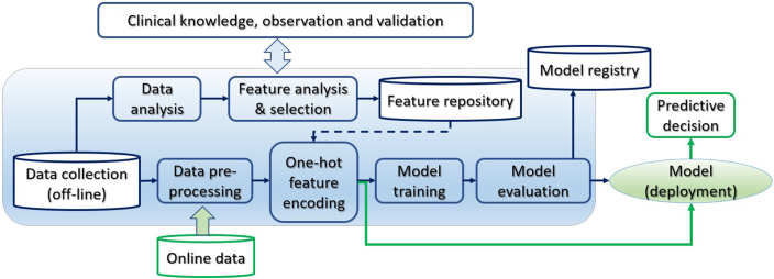
The clinical knowledge–enhanced ML pipeline has an end-to-end construct that codifies and facilitates the workflow to produce a scalable ML model. As shown in Figure 1, it consists of multiple sequential steps, from real-world clinical data input, data quality analysis, preprocessing, and feature extraction to model training, validation, and deployment. The pipeline engages clinical knowledge at each stage in the loop of AI model development. It is iterative to continuously improve the accuracy by selecting the best features and learning algorithms to build the best model for heart disease diagnosis. The widely used ML library Scikit-learn and Python were used to implement the pipeline and carry out the following experiments.

Figure 1.

The clinical knowledge–enhanced machine learning pipeline to build a predictive ischemic heart disease model.

Heart disease dataset

Medical health records usually contain a wealth of information; however, only relevant and discriminative attributes can be used for predictive analysis. The raw dataset consists of 303 records with 76 attributes and diagnosis labels from clinical professionals. It is from the Cleveland Clinic Foundation dataset and available online at the University of California, Irvine.⁸ Of the 76 attributes, medical experts used clinical knowledge to select the most relevant 13 attributes (index 1–13) and the target diagnostic IHD status (1-true or 0-false), as shown in Table 1. IHD positive is considered when the narrowing of at least 1 of the coronary arteries was more than 50%, as shown by coronary angiography. The used IHD dataset is well balanced with 165 (54.5%) positive IHD and 138 negative instances.

Table 1.

Clinical most relevant ischemic heart disease risk attributes

Index	Attribute	Definition	Data type
1	Age	Age in years	Numerical
2	Sex	Sex	Categorical 1: male, 0: female
3	cp	Chest pain type	Categorical 1: typical angina, 2: atypical angina, 3: non-anginal pain,4: asymptomatic
4	trestbps	Resting blood pressure	Numerical (mm Hg on admission to the hospital)
5	chol	Cholesterol	Numerical (mg/dL)
6	restecg	Resting electrocardiographic results	Categorical 0: normal, 1: having ST-T wave abnormality,2: showing probable or definite left ventricular hypertrophy by Estes’ criteria
7	thalach	Maximum exercise heart rate achieved	Numerical (71–202)
8	exang	Exercise-induced angina	Categorical 1: yes; 0: no
9	oldpeak	ST depression induced by exercise relative to rest	Numerical
10	slope	Slope of the peak exercise ST	Categorical 0: upsloping, 1: flat, 2: downsloping
11	ca	Number of major vessels colored by fluoroscopy	Categorical 0, 1, 2, 3
12	thal	Thallium-201 stress scintigraphy	Categorical 1: normal; 2: fixed defect; 3: reversible defect
13	fbs	Fasting blood sugar	Categorical (>120 mg/dL) 1: true; 0: false
14	target	Diagnosis of heart disease (angiographic disease status)	Categorical 0 = normal; 1 = IHD (>50% diameter narrowing)

IHD = ischemic heart disease.

Data visualization and analysis

Data analysis is an important process to validate the quality of data, inspect data properties, and discover useful information and features before starting ML. Data visualization is an effective way to explore vast amounts of data; gain an overview of data distribution; check class balance and missing or outlier data; and even discover potential patterns, trends, and clusters.

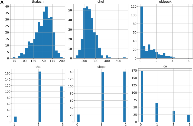
Using Matplotlib and Seaborn library with Python, we created various visualization charts, including histograms, swarm charts, and violin charts. As shown in Figure 2A, histograms of maximum exercise heart rate achieved (thalach) and cholesterol (chol) present a largely Gaussian distribution. The histogram of “oldpeak” presents a high occurrence of 0 ST depression induced by exercise relative to rest. This indicates minimal cardiac stress and is consistent with the large number of people in the database who do not have IHD, in whom we would not expect ECG changes in exercise. Categorical values and occurrence on thallium-201 stress scintigraphy (thal 1–3), slope of the peak exercise ST segment (1, 2), and number of major vessels colored by fluoroscopy (ca 0–3) are clearly presented. We can easily observe the outlier in chol above 550 mg/dL, the wrong value “0” in “slope,” and the out-of-range value “4” in “ca” attribute.

Figure 2.

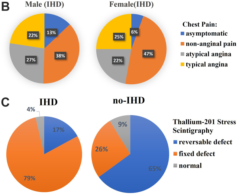
Data analysis and validation. A: Data distribution of maximum exercise heart rate achieved (thalach), cholesterol (chol), ST depression induced by exercise relative to rest (oldpeak), thallium-201 stress scintigraphy (thal) (1–3), slope of the peak exercise ST (1,2), and number of major vessels (0–3) colored by fluoroscopy (ca). B: Chest pain types for males and females with ischemic heart disease (IHD). C: Thallium-201 stress scintigraphy vs IHD.

Figure 2B shows the relative distribution of different chest pain symptoms experienced by male and female patients with diagnosed IHD. There appear to be similar proportions of men and women who experience typical and atypical angina.

As can be seen in Figure 2C, patients with IHD are more significantly likely to have a fixed defect on thallium-201 scintigraphy, whereas those without IHD are more likely to have a reversible defect. In both cases, the values for normal scintigraphy are low and almost negligible.

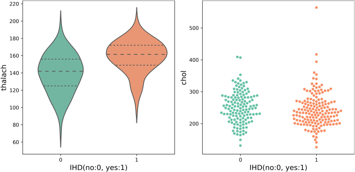
A violin plot is a hybrid of a box plot (basic summary statistics, eg, range and quartiles) and a kernel density plot to show the probability distribution of numerical data at different values. It is usually smoothed by a kernel density estimator. Figure 3 shows violin plots on maximum exercise heart rate achieved. The middle thick dashed line represents the median and 2 thin dashed lines indicate the interquartile range. We observed that people suffering from IHD have a higher average heart rate with exercise and at a higher probability (wider sections) than people without IHD.

Figure 3.

Maximum exercise heart rate achieved (thalach) (violin plot, left) and serum cholesterol (swarm chart, right), both vs ischemic heart disease (IHD) diagnosis.

A swarm chart is a scatterplot visualizing the distribution of an attribute or the joint distribution of a couple of discrete attributes. At each x location, the points are jittered based on the kernel density estimation in y; therefore the outline of each distinct shape is similar to a violin plot. In Figure 3 right, we observe that the distribution of serum cholesterol values in patients with IHD and those without is largely similar, where patients with IHD are grouped more tightly at a lower figure of around 240 mg/dL, whereas those without IHD are more spread out, with mean of around 250.

Data preprocessing using domain knowledge

To ensure the quality of learning, clinical domain knowledge is applied for preprocessing tasks, including missing data clean-up, dealing with outliers, and data standardization, as well as transforming and analyzing the data.

Missing data

Missing data are usually caused by, for example, data collection mistakes, people declining to give personal information, or an attribute that may not be applicable to all cases. With domain knowledge, missing data can be solved by (1) dropping the entire attribute when missing for more than 60% observations and this attribute is insignificant, (2) dropping instances, or (3) imputation, such as using median, mean, or a regression model to predict the missing data.

Outliers

Outliers are odd-one-out observations at an abnormal distance from the population group. Many learning algorithms are sensitive to the range and distribution of attribute values. Outliers should be excluded from the dataset when possible, since they represent different underlying behaviors or mistakes, thus skewing the training process and resulting in longer training times and less accurate models.

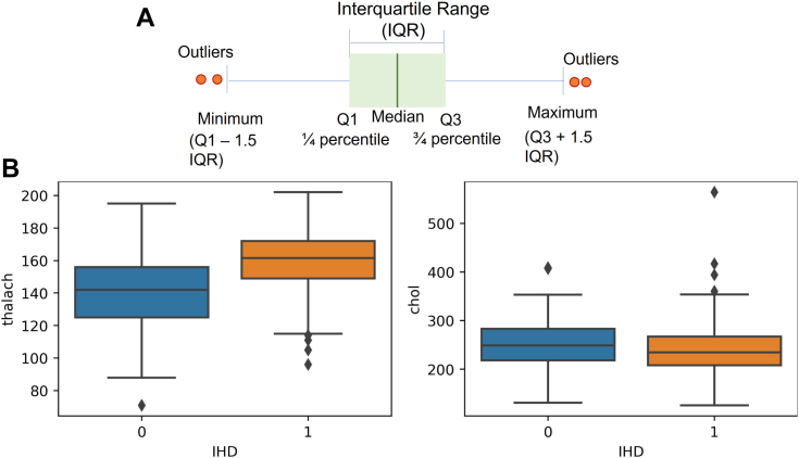
Data visualization is an effective way to identify outliers. As shown in Figure 4A, interquartile range (IQR) was used to detect outliers with numerical values. The IQR aims to represent the spread variability of the dataset. To calculate the IQR, the dataset is divided into rank-ordered even quartiles, denoted by Q1 (lower 25%), Q2 (median 50%), and Q3 (upper 75% quartile), so IQR is the median 50% (Q3 − Q1). The whiskers have an offset length of 1.5 × IQR; any data located outside of the whiskers is considered an outlier.

Figure 4.

Outlier detection using A: interquartile range (IQR) and B: box-and-whisker plots. IHD = ischemic heart disease.

Using box-and-whisker plots in Figure 4B we observed a few outliers in the “chol” and “thalach” attributes. In Figure 2A histograms, we can also easily observe the outlier in “chol” above 550 mg/dL, the wrong value “0” in “slope” (which could mean missing data), and 5 records with “ca” = 4 (number of major vessels colored by fluoroscopy) that are out the suggested database’s recording range (0,1,2,3). Based on domain knowledge, we removed some of these data points, and capped “ca” = 4 to 3 to maintain the dataset size.

In practice, we could completely remove outlier records, cap their values, or try to impute a new value. Domain knowledge and factors such as “how many” and “how far” of outliers should be considered when handling outliers.

Standardization

Some attributes have larger values and could dominate others although they are not important. Standardization aims to transform attributes to be fairly on a similar scale, thus improving model stability and speeding up training. Common techniques include min-max normalization, Z-scale, and log-scale.

For biomedical data, all attributes have a physiological range and many present as a normal or uniform distribution, such as blood pressure and heart rate. Therefore, we used Z-score standardization, since Z-score does not change the type of distribution. In practice, it is always possible to start by fitting models to raw, normalized, and standardized data, and compare the performance for best results.

Data-driven machine learning models

Machine learning–based feature selection

Recording medical data is complex and time-intensive. Irrelevant, redundant, or less discriminative variables degrade model generalization capability and accuracy. Adding more variables increases the model complexity, leading to high computational costs and overfitting risks. Feature selection aims to find the best set of informative features, and it hugely impacts the model performance.

Feature selection can be supervised or unsupervised. Supervised feature selection uses the target variable (eg, removing irrelevant variables using intrinsic, wrapper, filter, or hybrid methods). Intrinsic algorithms automatically learn feature importance during training, such as decision tree (DT) and RF. However, we did not find a consistent ranking result using such methods on the IHD dataset. Unsupervised feature selection does not involve the target variable (eg, removing redundant variables using variance threshold or correlation).

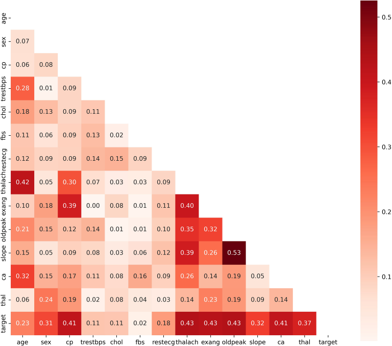
Correlation is one easy-to-implement and effective method for feature selection. It measures the linear relationship between variables. Discriminative variables should be highly correlated with the target, but less correlated with other input variables (reducing redundant information; eg, removing 1 of body mass index, weight, and height). In our experiment, Python Matplotlib and Seaborn were used to generate the correlation heat map among 13 variables, as shown in Figure 5. The Pearson threshold 0.6 was used to remove redundant features.

Figure 5.

Heat map on feature correlation in Pearson coefficients.

Meanwhile, Pandas corr() function with Pearson correlation coefficients and Scikit-learn SelectKBest() function with χ² test were used to rank the importance of 13 variables to IHD. As shown in Table 2, ranking results are very consistent. However, “fbs” has the lowest correlation to IHD, at almost 2 orders of magnitude less in χ² to the next attribute, while other features are largely within the same order of magnitude. The same applies to “fbs” under Pearson, but to a slightly lesser extent.

Table 2.

Feature correlation with ischemic heart disease using Pearson and χ² ranking

Index	Pearson		Index	χ2
	Attribute	Score [0,1]		Attribute	Score
1	oldpeak	0.4349	1	thalach	180.99
2	thalach	0.4337	2	ca	62.23
3	exang	0.4284	3	oldpeak	59.04
4	cp	0.4141	4	cp	51.82
5	ca	0.4112	5	exang	35.41
6	thal	0.3739	6	chol	29.21
7	slope	0.3246	7	age	22.81
8	sex	0.3114	8	sex	8.15
9	age	0.2278	9	slope	7.45
10	restecg	0.1820	10	trestbps	6.72
11	trestbps	0.1143	11	thal	5.72
12	chol	0.1119	12	restecg	4.69
13	fbs∗	0.0176	13	fbs∗	0.08

The attribute “fbs” measures fasting blood sugar, and thus is used to diagnose diabetes in patients. As diabetes is a known risk factor for IHD, it would be expected for a stronger correlation. However, patients with diabetes will usually be on medications/diets to control their blood sugar levels, so they correspondingly may not have elevated fbs. Only those who were undiagnosed or had poor control of blood sugars would have high fbs. Furthermore, fbs uses a binary value in the dataset through a cut-off value for blood sugar, thus degrading its representation and discriminative ability compared to a true numerical measure. Therefore, it could be argued that “fbs” could be removed from mode results using data-driven ML models

After data preprocessing, 282 patient records (70% male, 56% IHD positive) remained out of the original 303 records. The dataset is randomly split into 75% for training and 25% “hold-out” for testing. The 25% testing data was not used in model training.

Twelve selected attributes (excluding “fbs”) were used for model training. Six widely used learning algorithms, DT, RF, KNN, naïve Bayesian, SVM, and artificial neural network (ANN), were well fine-turned and evaluated to determine the best model.

Table 3 compares the performance of 6 ML models. For evaluation, 5 clinically important performance matrices were used, including accuracy, precision, sensitivity (recall), specificity, and F1 score. The average accuracy of the 6 models was improved to 85% compared with 83.5% when using the original 13 attributes. ANN achieved the best accuracy (88.7%), precision (85%), specificity (82%), and F1 score (90%), while SVM achieved the highest sensitivity (97%).

Table 3.

Comparison of learning algorithms on original 12 ischemic heart disease attributes

Models	12 original features (removing fbs)
	Accuracy	Precision	Recall	F1 score
DT	0.816	0.80	0.86	0.83
RF	0.831	0.79	0.92	0.85
KNN	0.845	0.80	0.95	0.86
Naïve Bayesian	0.845	0.82	0.89	0.86
SVM	0.873	0.82	0.97∗	0.89
ANN	0.887∗	0.85∗	0.95	0.90∗
Average	0.850	0.81	0.92	0.87

ANN = artificial neural network; DT = decision tree; KNN = k-nearest neighbor; RF = random forest; SVM = support vector machine.

^∗Indicates the highest value in accuracy, precision, recall and FI.

DT-based learning produces a hierarchical tree-like model with better interpretability. DT predicts a target variable by learning simple decision rules inferred from the inputs. At each node, it searches for the best feature and its threshold that splits the data into 2 subsets, aiming to produce the purest subsets with maximum information gain. There are different criteria to maximize information gain at each tree node, such as Gini and Entropy. As shown in Figure 6, the learned tree model can be presented graphically, thus visually and explicitly representing a piecewise constant decision-making process. Whether this ML DT is consistent with what can be explained clinically will be addressed in the Discussion section.

Figure 6.

Decision tree of top 5 layers using 12 original attributes. X index order is consistent with the top 12 attributes in Table 1, but starts from 0.

In our experiments, each model has been fine-tuned for its best performance to compare with others. For DT learning, we found that Gini overperformed Entropy to evaluate information gain, and achieved 81.6% accuracy. We experimented with different numbers of trees to determine 60 estimators for RF at its maximum accuracy of 83.1%. We found that KNN with k = 7 achieved smooth decision boundaries and the best accuracy (84.5%) compared to all others. Typical naïve Bayesian probability includes Gaussian, multinomial, and Bernoulli. According to our experiments, Bernoulli achieved the best accuracy (84.5%) among the 3 Bayesian models. We experimented with several typical SVM kernels including linear, radial basis function, Poly, and Sigmoid. The highest SVM accuracy (87.3%) was achieved by using Sigmoid.

The neural network model achieved top accuracy of 88.7% among others. The network consists of 1 input layer with 12 neurons, 1 dense hidden layer with 8 neurons activated by ReLU, and an output layer using Sigmoid activation for binary classification. Binary_crossentropy was used for the loss function with Adam as its optimizer. The network was trained with 100 epochs at a learning rate of 0.001. We found adding more hidden layers (deep neural network) degraded network accuracy, largely because the dataset is small relative to model complexity with a deep structure.

Embedding clinical knowledge into data-driven model learning

So far we have demonstrated model performance using a largely data-driven ML approach. This creates a baseline for us to compare with a more clinically engaged approach. Although some domain knowledge has been introduced in data analysis and preprocessing, feature selection has been generally based on statistical principles. In this section, we present model improvements by introducing one-hot encoding to break down features and thus allow further incorporation of clinical knowledge for crucial feature selection. Meanwhile, we also incorporate clinical input to identify and eliminate data bias in model learning.

One-hot encoding and improvements in feature selection

Clinical data attributes often include categorical data with several conceptual values. For example, thallium-201 stress scintigraphy contains 3 different conceptual values: thal_1 (normal); thal_2 (fixed defect); thal_3 (reversible defect). From clinical knowledge, we know that “thal” is very useful in diagnosing IHD, in particular the fixed and reversible defects. However, thal ranks relatively low in our statistical feature ranking in Table 2 (6th in Pearson and 11th in χ²).

To explore issues where there is discordance between clinical expectation and ML feature ranking, we introduce one-hot encoding to break down features into their constituent parts. This allows the most discriminative categorical values (ie, thal_2 and thal_3) to stand out and contribute more effectively to model learning.

At the same time, most learning algorithms require the conversion of categorical data to integers. The order of numbers naturally introduces an attribute of significance, thus adding bias to variables without ordinal relationships. In contrast, the proposed one-hot encoding converts each categorical value into a new categorical column feature and assigns a binary value of 1 or 0. One-hot encoding thus not only allows us to break down the data features to be more interpretable, but also removes feature coding bias.

In our study, one-hot encoding was applied to 3 categorical variables, including (1) chest pain cp_0–cp_3 (typical angina, atypical angina, non-anginal pain, asymptomatic, respectively); (2) slope of the peak exercise ST segment slope_0–slope_2 (upsloping, flat and downsloping); and (3) thallium-201 stress scintigraphy thal_1–thal_3 (normal, fixed defect, and reversible defect). One-hot feature ranking using Pearson and χ² test is shown in Table 4.

Table 4.

Feature ranking on one-hot encoded features using Pearson and χ² test

Index	Pearson (one-hot)		Index	χ2 (one-hot)
	Attribute	Score [0,1]		Attribute	Score
1	thal_2	0.5387	1	thalach	180.99
2	cp_0	0.5059	2	ca	62.23
3	thal_3	0.5000	3	oldpeak	59.04
4	oldpeak	0.4349	4	thal_3	44.24
5	thalach	0.4337	5	cp_0	39.16
6	exang	0.4284	6	exang	35.41
7	ca	0.4112	7	thal_2	35.40
8	slope_2	0.3751	8	chol∗	29.21
9	slope_1	0.3625	9	Age∗	22.81
10	Sex∗	0.3114	10	slope_2	20.40
11	cp_2	0.2998	11	slope_1	20.10
12	cp_1∗	0.2554	12	cp_2	17.98

^∗Indicates no overlapping attributes in Pearson and χ².

We can observe that thal_2 and thal_3 are now able to be ranked a lot higher. The attribute cp_0 can also be differentiated from the lower-ranked cp_1 and cp_2, while cp_3 did not even rank in the top 12 one-hot features. This largely fits with clinical observations. Similarly, the importance of the 3 categorical factors in “slope” can be better demonstrated. We also observe that there is a significant degree of 83% concordance between χ² and Pearson of the top 12 one-hot ranked features.

For comparison with data-driven ML models using 12 attributes, the top 12 one-hot features were used to train the 6 models. Using 12 one-hot features, average accuracy on χ² ranking achieved 88.7%, as shown in Table 5, and on Pearson ranking was 87.5%, both higher than 83.8% using original 13 attributes and 85% using selected 12 variables.

Table 5.

Comparison of learning algorithms on reduced one-hot encoded features

Models	12 one-hot features					7 one-hot features
	Accuracy	Precision	Recall	Specificity	F1 score	Accuracy	Precision	Recall	Specificity	F1-score
DT	0.761	0.83	0.72	0.81	0.77	0.775	0.82	0.78	0.77	0.79
RF	0.873	0.94	0.82	0.94	0.88	0.873∗	0.9	0.88	0.87	0.89
KNN	0.929∗	0.95∗	0.93∗	0.94∗	0.94∗	0.929	0.97	0.9	0.97∗	0.94
Naïve Bayesian	0.915	0.95	0.9	0.94	0.92	0.915	0.97	0.88	0.97∗	0.92
SVM	0.929∗	0.95∗	0.93∗	0.94∗	0.94∗	0.944∗	0.95∗	0.95∗	0.94	0.95∗
ANN	0.915	0.95	0.9	0.94	0.92	0.901	0.95	0.88	0.94	0.91
Average	0.887	0.93	0.87	0.92	0.90	0.890	0.93	0.88	0.91	0.90

ANN = artificial neural network; DT = decision tree; KNN = k-nearest neighbor; RF = random forest; SVM = support vector machine.

^∗Indicates the highest accuracy value for each measurement.

Recognizing data bias and model improvement with clinical input

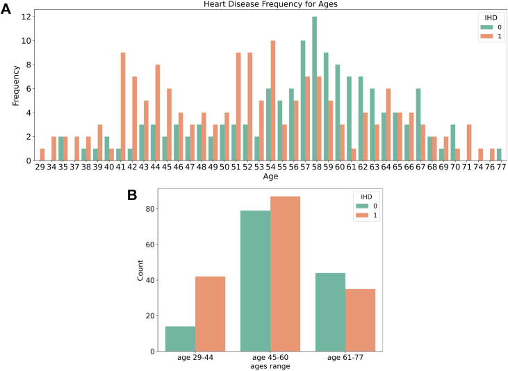
Medical domain knowledge was applied to identify possible inaccuracies and biases in the data. In Figure 7, the ages and IHD status of people in our dataset are visualized using a histogram. We observe that non-IHD patients have a normal Gaussian distribution with a mean age of around 58, while IHD patients appear to have 2 peaks around 41–44 and 54. This distribution is at odds with what might be expected clinically, as advancing age is a well-known risk factor for IHD. This demonstrates an example of data bias that was recognized using clinical expertise. Possible explanations include a lack of sufficient data points (only 303) to cover the wide range of ages and sampling errors in the original dataset, meaning the population in the dataset is not representative of the population as a whole. It may also be an artefact of the database creating a balanced sample of having roughly half of its patients having IHD and half without. Many learning algorithms are more robust with variables of limited values. For small datasets, it can thus be particularly beneficial to discretize continuous values into limited categorical values, for example, converting ages into ordinal-scale variables (eg, young adults: 29–44, middle-aged adults: 45–60, and older adults: 60+, as shown in Figure 7B).

Figure 7.

Ischemic heart disease (IHD) occurrence with age. A: IHD occurrence at different ages. B: IHD occurrence in 3 age groups.

Figure 3 (right) showed that the distribution of serum cholesterol values in patients with IHD and those without was largely similar. Cholesterol values of patients with IHD appear to be more clustered at a lower figure, around 240 mg/dL, whereas those without IHD is more spread out, with a mean of around 250. This is not what would be clinically expected, as blood cholesterol is a major contributor to build-up of atherosclerotic plaques that cause IHD. Two possible explanations may be the fact that total cholesterol is used, not differentiating between HDL (“good cholesterol”) and LDL (“bad cholesterol”); and that patients who are diagnosed with IHD are more likely to be on cholesterol-lowering medications, which may also explain why the data are more clustered than the non-IHD group. Overall, these biases in the data could degrade the consistency and stability of the model. Such biases may not be identified without clinical domain knowledge.

To combat these examples of data bias, we removed age and cholesterol from the 12 one-hot features. Furthermore, from clinical consensus, slope was deemed to be relatively less discriminative. Experiments with this clinical input of removing slope_1 and slope_2 showed improved model performance. This means a total of 4 features were removed. Further experiments were conducted with 6, 7, and 8 one-hot features. It was found the optimal set of 7 one-hot features improved average model accuracy to 89%, in comparison to 88.7% using 12 one-hot features, as shown in Table 5. The SVM (linear kernel) and KNN overperformed the other models. By using only 7 one-hot encoded features, the SVM achieved the top overall performance with accuracy 94.4%, precision 95%, sensitivity 95%, specificity 94%, and F1 95%, while the KNN achieved the highest specificity (97%).

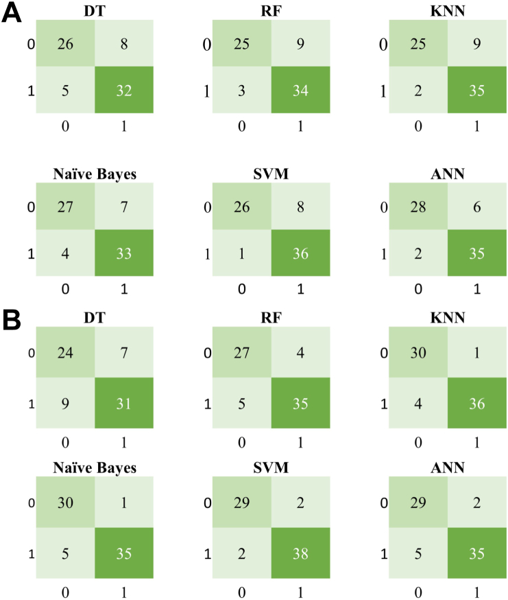
Among these experiments we found SVM, ANN, and KNN have better performance in general, eg, SVM 88.7% and ANN 87.3% on 13 original attributes; ANN 88.7% and SVM 87.3% on 12 selected features; SVM and KNN keep top on one-hot encoded reduced features (Tables 3 and 5). As shown in Figure 8, confusion matrices present how the 6 learning algorithms could be confused with IHD-positive and IHD-negative classes. Each row of the matrix represents the instances in an actual class, while each column represents the instances in a predicted class.

Figure 8.

Confusion matrices for 6 learning algorithms, with 1 indicating ischemic heart disease (IHD)-positive and 0 IHD-negative classes. A: Using 12 original IHD attributes. B: Using 7 one-hot encoded features. ANN = artificial neural network; DT = decision tree; KNN = k-nearest neighbor; RF = random forest; SVM = support vector machine.

Comparison of clinical knowledge–enhanced ML pipeline with state-of-the-art data-driven ML

To our knowledge, this is the first study that explores the mechanism of how to embed clinical expertise in an ML pipeline, and evaluates its impact on model performance. We therefore compared the proposed clinical knowledge–enhanced ML pipeline method with 6 state-of-the-art conventional data-driven ML models without clinical input. The results, based on the benchmark Cleveland Clinic Foundation dataset, are shown in Table 6. Our clinician-enhanced SVM model achieved the best accuracy of 94.4%, as well as competitive performance on precision, recall, specificity, and F1 score.

Table 6.

Comparison with existing machine learning models on benchmark Cleveland ischemic heart disease dataset

Models	Accuracy
RBF kernel-based SVM14	82.18%
Fuzzy rule-based model15	84.00%
Logistic regression SVM16	84.85%
Hybrid random forest17	88.40%
Ensemble model18	90.00%
Neural network with hyper-parameter optimization19	90.78%
Our clinical knowledge–enhanced ML model	94.40%

ML = machine learning; RBF = radial basis function; SVM = support vector machine.

Furthermore, our model used only 7 one-hot encoded IHD attributes, compared with other methods. It demonstrates that embedding clinical knowledge to select fewer, more discriminative features can improve model performance, even with fewer total features used.

Discussion

Performance metrics

Accuracy is a useful measure when false-negative and false-positive counts are similar and they have similar cost impacts. Precision indicates the level of certainty regarding true-positives; it is used when we need to be more confident about true-positives. It is about how sure we are that we do not miss any positives. F1 is the harmonic average of the precision and sensitivity; it is more meaningful if precision and recall are more balanced. In practice, F1 is a better indicator when the costs of false-positives and false-negatives are very different, or if class distribution is very uneven.

In medical tests, sensitivity is the ability of the test to correctly identify those with the disease, in this case IHD. On the flip side, specificity is the ability of the test to correctly identify those without the disease. Often, having a single test that is both highly sensitive and specific is not possible. In such cases it becomes desirable to prioritize, balancing the cost impact of missing a true diagnosis against creating a false-positive diagnosis. In the case of IHD, it could be argued that sensitivity is the more important of the two, as missing a diagnosis and not starting treatment could be considered worse than preemptively starting treatment in those without the disease. Clearly, this consideration must be modulated by the size of the difference in specificity and sensitivity, and the purpose/population that is being screened. For example, a test looking for IHD in a small but high-risk group needs to be highly sensitive, but a screening test for the whole population would require a higher specificity to prevent masses of false-positive results. Thus often in clinical medicine, 2 or more tests can be used in sequential order to produce an overall diagnosis that is more accurate.

Table 5 shows that SVM using 7 one-hot features achieved good performance, which means measured by accuracy 94.4%, precision 95%, sensitivity 95%, and F1 95%. These means the following: (1) 94.4% (accuracy) of SVM-produced IHD diagnosis results are correct; (2) on average, 95% (precision) of patients labeled by the SVM model is true IHD; and (3) 95% (sensitivity) of IHD patients in reality are flagged, but 5% IHD patients are missed.

Breaking down the “black box” and embedding clinical knowledge

Many clinicians remain cautious of AI owing to longstanding concerns about “black box” models. “Black box,” in a general sense, means that models and their operations can be very complex, not visible, and not straightforwardly interpretable to humans. Understanding how AI models work is essential to gain trustworthiness in AI decision-making in the medical domain.

To address this issue, the proposed work introduces a transparent ML pipeline, thereby breaking down the black box into its constituent parts. This allows us to identify, explain, and see if we can intervene using clinical knowledge and evaluate its impact on model performance.

A summary of how clinical input is applied, as well as the corresponding improvement in model performance, is shown in Table 7. The average shown is the average accuracy over 6 ML models in the section on experimental results using data-driven ML models. It is useful to note that the 12 one-hot encoded features contain fewer total values than the original 12 features, which have more categorical values. This allowed us to explore the impact of individual categorical attributes and reduce overall features.

Table 7.

Model improvement benefited from clinical input at different stages of the machine learning pipeline

Features	Clinical knowledge	Average accuracy
13 attributes	Clinical experts (database creators) selected 13 most relevant attributes from 72.	83.5%
12 features	Clinical knowledge was used in data preprocessing to address outlier and missing data points, as well as to remove the statistically and clinically insignificant attribute “fbs.”	85.0%
12 one-hot features	Identifying that clinically relevant features are not fully exposed (eg, thal). One-hot encoding was introduced to expand categorical attributes. The best feature set can thus be selected.	88.7%
7 one-hot features	Clinical input was used to recognize data bias (eg, age), as well as less significant features (eg, slope), and remove them from model learning.	89.0 % (94.4% with SVM)

SVM = support vector machine.

An important observation is that at each stage, while the total number of features is reduced, model performance is increased. This is generally not easy to gain from standard data-driven ML processes. This lack of accuracy decay improvement strongly suggests information gain from the clinical domain knowledge we are embedding. Furthermore, removing less discriminative features from can reduce potential clinical test costs and workload for recording these measures.

In terms of learning algorithms, DT presents better interpretability among others. As shown in Figure 6, chest pain (“cp”) is used at the first root split with information gain of 0.489, then “ca,” “thal,” “oldpeak,” etc are used in the following decision layers. This decision-making hierarchy is generally consistent with feature ranking (Table 2) as well as our final 7 one-hot selected features. These features are also consistent with the clinically most objectively reliable features. For example, the most invasive but diagnostic features, “ca” and “thal,” obtained by invasive imaging, are both placed very highly in the DT. On the other hand, less diagnostic features such as “exang” or “trestbps,” which require only a clinical history or simple bedside measurements like blood pressure, are placed lower in the tree. Features requiring a moderate amount of cost and corresponding diagnostic ability, such as “oldpeak,” which looks at ECG changes during exercise, or “thalach,” which looks at maximum exercise heart rate achieved, are generally found in the middle of the tree. The one exception is at the top of the tree, where “cp” (chest pain) is found. This is purely derived from clinical history and its position matches its position at the top of a clinician’s DT when deciding the risk of IHD when taking a clinical history. Overall, the ML DT uses the most diagnostic features first, but these are often also invasive and costly. Thus a clinician’s DT, which factors cost and risk to patients from invasive procedures, will have to consider the less invasive procedures first, relying on invasive tests at the end to confirm the diagnosis.

Conclusion

IHD has considerable impact on health, but its impact can be reduced if the possibility of heart disease occurrence can be assessed earlier. We presented the first clinical knowledge–enhanced ML model for predicting IHD. We explored the mechanisms at different stages of the ML pipeline, allowing us to incorporate clinical expertise and improve model performance. This included key steps such as data analysis, preprocessing, feature selection, and model learning evaluation. We introduced a novel one-hot encoding method, allowing us to expose hidden bias in categorical attributes and identify clinically discriminative elements and features.

Experimental results demonstrated improvement in model accuracy by embedding clinical knowledge. Using the benchmark Cleveland IHD dataset, the best model based on SVM achieved an accuracy of 94.4%, precision 95%, sensitivity 95%, and F1 95% by using 7 one-hot encoded features. This result outperforms the state-of-the-art data-driven ML models. It also represents a 63% reduction in clinical recording compared with using 13 attributes and more values for categorical attributes.

The main contribution of our work is to explore the mechanism of embedding clinical knowledge in conventional “black box” ML. Although the benchmark dataset we can currently access is relatively small, it still demonstrates the effectiveness of the proposed approach. In the future, we hope the wider research community can build on our exploratory study and adapt this approach on larger datasets, leading to a fully evaluated predictive IHD model for clinical use.

References

- 1.Dai H., Much A., Maor E., et al. Global, regional, and national burden of ischaemic heart disease and its attributable risk factors, 1990–2017: results from the Global Burden of Disease Study 2017. Eur Heart J Qual Care Clin Outcomes. 2022;8(1):50–60. doi: 10.1093/ehjqcco/qcaa076. [DOI] [PMC free article] [PubMed] [Google Scholar]
- 2.Khan M.A., Hashim M.J., Mustafa H., et al. Global epidemiology of ischemic heart disease: results from the Global Burden of Disease Study. Cureus. 2020;12(7):e9349. doi: 10.7759/cureus.9349. [DOI] [PMC free article] [PubMed] [Google Scholar]
- 3.Tavakol M., Ashraf S., Brener S.J. Risks and complications of coronary angiography: a comprehensive review. Glob J Health Sci. 2012;4(1):65. doi: 10.5539/gjhs.v4n1p65. [DOI] [PMC free article] [PubMed] [Google Scholar]
- 4.Morrow D.A. Cardiovascular risk prediction in patients with stable and unstable coronary heart disease. Circulation. 2010;121(24):2681–2691. doi: 10.1161/CIRCULATIONAHA.109.852749. [DOI] [PubMed] [Google Scholar]
- 5.Johnson K.W., Torres Soto J., Glicksberg B.S., et al. Artificial intelligence in cardiology. J Am Coll Cardiol. 2018;71(23):2668–2679. doi: 10.1016/j.jacc.2018.03.521. [DOI] [PubMed] [Google Scholar]
- 6.Cuocolo R., Perillo T., De Rosa E., Ugga L., Petretta M. Current applications of big data and machine learning in cardiology. J Geriatr Cardiol. 2019;16(8):601. doi: 10.11909/j.issn.1671-5411.2019.08.002. [DOI] [PMC free article] [PubMed] [Google Scholar]
- 7.Garcia-Canadilla P., Sanchez-Martinez S., Crispi F., Bijnens B. Machine learning in fetal cardiology: what to expect. Fetal Diagn Ther. 2020;47(5):363–372. doi: 10.1159/000505021. [DOI] [PubMed] [Google Scholar]
- 8.Cleveland Clinic Foundation heart disease dataset. https://archive.ics.uci.edu/ml/datasets/heart+disease
- 9.Kitlas Golínska A., Lesínski W., Przybylski A., Rudnicki W.R. Computational Science – ICCS 2020, 20th International Conference, Amsterdam, The Netherlands, June 3–5, 2020, Proceedings, Part VI. Springer; 2020. Towards prediction of heart arrhythmia onset using machine learning; pp. 376–389. [Google Scholar]
- 10.Uyar K., Ilhan A. Diagnosis of heart disease using genetic algorithm based trained recurrent fuzzy neural networks. Procedia Computer Science. 2017;120:588–593. [Google Scholar]
- 11.Cheng C.-A., Chiu H.-W. An artificial neural network model for the evaluation of carotid artery stenting prognosis using a national-wide database. Annu Int Conf IEEE Eng Med Biol Soc. 2017;2017:2566–2569. doi: 10.1109/EMBC.2017.8037381. [DOI] [PubMed] [Google Scholar]
- 12.Khourdifi Y., Bahaj M. Heart disease prediction and classification using machine learning algorithms optimized by particle swarm optimization and ant colony optimization. International Journal of Intelligent Engineering and Systems. 2019;12(1):242–252. [Google Scholar]
- 13.Rathnayakc B, Ganegoda G. Heart diseases prediction with data mining and neural network techniques. In: 2018 3rd International Conference for Convergence in Technology (I2CT), pp. 1–6.
- 14.Shah S.M.S., Batool S., Khan I., Ashraf M.U., Abbas S.H., Hussain S.A. Feature extraction through parallel probabilistic principal component analysis for heart disease diagnosis. Physica A: Statistical Mechanics and its Applications. 2017;482:796–807. [Google Scholar]
- 15.Marateb R., Goudarzi S. A noninvasive method for coronary artery diseases diagnosis using a clinically-interpretable fuzzy rule-based system. J Res Med Sci. 2015;20(3):214. [PMC free article] [PubMed] [Google Scholar]
- 16.Bashir S, Khan ZS, Hassan Khan F, Anjum A, Bashir K. Improving heart disease prediction using feature selection approaches. 2019 16th International Bhurban Conference on Applied Sciences and Technology (IBCAST), pp. 619–623.
- 17.Mohan S., Thirumalai C., Srivastava G. Effective heart disease prediction using hybrid machine learning techniques. IEEE Access. 2019;7:81542–81554. [Google Scholar]
- 18.Atallah R., Al-Mousa A. Heart disease detection using machine learning majority voting ensemble method. International Conference on New Trends in Computing Sciences (ICTCS) 2019;1–6 [Google Scholar]
- 19.Sharma S., Parmar M. Heart diseases prediction using deep learning neural network model. International Journal of Innovative Technology and Exploring Engineering. 2020;9(3):124–137. [Google Scholar]
Associated Data
This section collects any data citations, data availability statements, or supplementary materials included in this article.