Fluorescence lifetime image microscopy prediction with convolutional neural networks for cell detection and classification in tissues

Justin A Smolen; Karen L Wooley

doi:10.1093/pnasnexus/pgac235

. 2022 Oct 14;1(5):pgac235. doi: 10.1093/pnasnexus/pgac235

Fluorescence lifetime image microscopy prediction with convolutional neural networks for cell detection and classification in tissues

Justin A Smolen ^1,^✉, Karen L Wooley ²

Editor: Amalio Telenti

PMCID: PMC9802238 PMID: 36712353

Abstract

Convolutional neural networks (CNNs) and other deep-learning models have proven to be transformative tools for the automated analysis of microscopy images, particularly in the domain of cellular and tissue imaging. These computer-vision models have primarily been applied with traditional microscopy imaging modalities (e.g. brightfield and fluorescence), likely due to the availability of large datasets in these regimes. However, more advanced microscopy imaging techniques could, potentially, allow for improved model performance in various computational histopathology tasks. In this work, we demonstrate that CNNs can achieve high accuracy in cell detection and classification without large amounts of data when applied to histology images acquired by fluorescence lifetime imaging microscopy (FLIM). This accuracy is higher than what would be achieved with regular single or dual-channel fluorescence images under the same settings, particularly for CNNs pretrained on publicly available fluorescent cell or general image datasets. Additionally, generated FLIM images could be predicted from just the fluorescence image data by using a dense U-Net CNN model trained on a subset of ground-truth FLIM images. These U-Net CNN generated FLIM images demonstrated high similarity to ground truth and improved accuracy in cell detection and classification over fluorescence alone when used as input to a variety of commonly used CNNs. This improved accuracy was maintained even when the FLIM images were generated by a U-Net CNN trained on only a few example FLIM images.

Keywords: fluorescence lifetime imaging microscopy, convolutional neural networks, computational histology, machine learning

Significance Statement.

Computational histopathology has benefited greatly from recent advances in computer vision and deep learning, allowing for automated analysis of various cellular and tissue features. However, most of the work has been focused on improving computer-vision models for datasets using standard imaging techniques. This work explores the benefit of applying these advanced models in the domain of fluorescence lifetime imaging microscopy (FLIM). The superiority of FLIM to standard fluorescence imaging is demonstrated for common computer-vision tasks. Additionally, the possibility of generating predictions of FLIM from standard fluorescence is explored and demonstrated to also improve computer-vision model accuracy.

Introduction

The ability to accurately locate, classify, and segment cells within microscopy images is fundamental for bioimaging applications in both basic and translational biomedical research, as it enables the study of cell spatial relationships and morphologies as they pertain to physiology, drug response, and disease (1, 2). Automating these otherwise time-consuming and expert-dependent tasks has been an active area of research and development (3, 4), particularly since the advent of convolutional neural networks (CNNs), which have attained substantially higher accuracies than previous “hand-crafted,” feature-engineered methods (5). Fluorescence tissue imaging presents a number of challenges that can reduce the accuracy of CNNs in cell segmentation and classification, including auto-fluorescence, dense clustering, and variation in cell size, shape, and density among different cell types (6). Much of the effort in overcoming these challenges has been focused on improving CNN architectures or creating large datasets for pretraining CNNs so that they attain high accuracies with limited training examples (4, 6–8). However, improvements may also be made by leveraging advances in microscope technology for use in combination with CNNs or other deep-learning architectures.

Fluorescence lifetime imaging microscopy (FLIM) records the exponential fluorescence decay response following excitation with a pulsed or time-modulated light source (9). If they have different lifetime decays, multiple fluorophores can be separated by FLIM, even when they have similar excitation and emission profiles (10–12). Thus, FLIM provides an extra dimension of contrast in fluorescence imaging that may be leveraged to reduce issues with auto-fluorescence (13)—a common problem in fluorescence tissue imaging (14, 15)—as well as for multiplexing of multiple stains under the same spectral acquisition settings (16). Fluorescence lifetimes may also vary depending on the molecular environment, which can provide additional contextual information, such as the pH (17), viscosity (18), polarity (19, 20), and concentration of ionic species (21–23). In some cases, FLIM responses of various fluorophores to microenvironmental conditions have been shown to have cell and tissue-specific patterns, which may be used for detection and classification (24–28).

In this work, we explored the advantages that FLIM provides for a variety of CNN architectures for cell instance segmentation and classification in tissue imaging. FLIM images were acquired on mouse lung tissue sections stained with spectrally overlapping nuclear and cell-membrane stains in order to take advantage of FLIM contrast. FLIM raw data are typically stored in various formats that depend on the instrumentation and whether the acquisition was performed in the time domain (e.g. time-correlated single-photon counting) or frequency domain. Therefore, to provide a generalizable method for FLIM representation, acquired time-domain lifetime decays were transformed to their two phasor components (g and s), applicable for both time- and frequency-domain FLIM (29). Most CNN architectures have been developed for use with regular red, green, and blue (RGB) images, so methods to translate the phasor FLIM data to RGB were also explored. Since FLIM provides both the integrated fluorescence signal as well as the decay response, CNN accuracies when trained with and without lifetime information were compared on the same set of images. The addition of lifetime information improved CNN accuracy for both cell instance segmentation and classification across all architectures tested when compared with conventional single and dual-channel fluorescence. In many cases, the improvement in accuracy with the addition of FLIM was more pronounced for the highest-performing CNN architectures that were pretrained on publicly available datasets.

While FLIM can provide several advantages for bioimaging, it comes at the cost of longer acquisition times (30) and, in the case of time-domain FLIM, large storage requirements for the raw data (31). The throughput for imaging large sections of tissue by FLIM, for instance, for whole-slide scanning, is thus substantially lower than for conventional fluorescence imaging (30). As a proposed solution to increase throughput, a dense U-Net CNN architecture was adapted to predict the phasor FLIM images using only single or dual-channel fluorescence images as input. The U-Net CNN generated FLIM images were not only highly similar to ground-truth, but also conferred similar advantages over fluorescence alone for cell instance segmentation and classification with CNNs. In particular, FLIM images generated using dual-channel fluorescence input were almost at par with ground-truth FLIM in many instances and required few training examples. This method could, thereby, allow for only a subset of images to be acquired by FLIM during an experiment while the others are acquired via regular fluorescence, while still maintaining most of the advantages of employing FLIM for all images.

Results

FLIM acquisition was conducted upon wild-type mouse (Balb-C) lung tissues that had been cryosectioned (10 µm), mounted, fixed, and stained using a combination of propidium iodide (PI) and Alexa-Fluor 555 conjugated wheat-germ agglutinin (WGA). These stains were chosen as they have overlapping excitation and emission wavelengths but separable fluorescence lifetimes, providing FLIM contrast for the nuclei (PI) and cell membranes (WGA). FLIM acquisitions were made using a fluorescence-lifetime equipped confocal microscope (Leica SP8 FALCON) of eighty different areas of tissue at two excitation/emission wavelengths: 570/575 to 620 nm and 590/600 to 640 nm. FLIM data from each wavelength displayed contrast for both nuclei and membranes, with 570 nm excitation displaying higher fluorescence intensity for the cell membranes and 590 nm excitation highlighting the nuclei.

FLIM data were transformed from the time domain using the phasor approach, yielding three components for each pixel coordinates ( Inline graphic ):

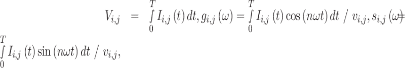where Inline graphic is the integrated intensity, and are the phasor components (x and y on the phasor plot), is the number of photons at a given decay time t, n is the harmonic frequency (, for first harmonic), and is the angular frequency (, where f is the laser repetition frequency) (32). Phasor FLIM is often calibrated with a reference fluorophore sample of known, mono-exponential lifetime (29). However, in this application, the actual lifetimes are not needed and calibration to fit the universal semicircle is redundant, as the values are all normalized to a range determined by the measured signal to convert to an RGB image (see the “Material and Methods” section).

Three methods were explored for translating phasor FLIM image data into three-channel (RGB) FLIM images for input into computer-vision models: directly to RGB from each of the three phasor-FLIM channels; via hue, saturation, value (HSV) color space transformation of the g and s components and fluorescence integrated intensity, respectively; or by first reducing the phasor components into one dimension using linear discriminant analysis (LDA) (33) and using that as the hue (H) and the fluorescence intensity as the value (V) with the saturation at maximum (LDA + HV, see the “Material and Methods” section). The HSV transformations reduce the contrast of low-intensity pixels, which have fewer photon counts and thus higher error in fluorescence lifetime. Consequently, the HSV- (Supplementary Material Appendix Fig. S1) and LDA + HV-transformed (Fig. 1A) RGB images are similar to commonly employed FLIM contrast visualization methods, while the direct RGB images display substantial levels of background noise (Supplementary Material Appendix Fig. S1).

Fig. 1. — Comparison of colorized FLIM and regular fluorescence confocal images on cell detection. (A) FLIM images of mouse lung sections stained with PI and WGA for nuclei and cell membrane, respectively, imaged for fluorescence lifetime at ex./em. 570/575 to 620 nm (top) and 590/600 to 640 nm (bottom) and visualized using LDA to reduce the phasor signal to one dimension to determine pixel hue, which was then combined with the fluorescence intensity signal to form an RGB image. (B) Evaluation of cell detection average precision by intersection over union (IoU) of Mask R-CNN with a ResNet-50 backbone trained using single (gray) or dual channel (black) regular fluorescence images or FLIM images using either direct HSV colorization of the phasor components (green), LDA then HV colorization (red), or direct conversion of phasor and fluorescence intensity to RGB channels (purple). Horizontal dot-dashed lines represent the average precision of the best model at IoU = 0.7, with the color signifying the type of training images used.

Comparison of FLIM and fluorescence images for cell detection and classification

Annotation masks on the cell nuclei and corresponding cell-class labels were made for twenty FLIM image sets. Cell detection was posed as an instance segmentation problem, such that the models must both detect the presence/location of the cell nuclei and label the pixels associated with the nuclei. Models were trained with either fluorescence intensity image inputs (single- or dual-channel) or FLIM inputs (single-channel only) using one of the RGB transformation methods. Prior to training, model weights were either randomly initialized or loaded from the same models trained on fluorescent cells from the Data Science Bowl 2018 (DSB) dataset (7). Comparisons were made for three model architectures: Mask R-CNN with a ResNet-50 backbone (Fig. 1B) and a ResNet-101 backbone (Supplementary Material Appendix Fig. S2A) (34, 35), and Stardist (Supplementary Material Appendix Fig. S2B) (36). The average precision of the instance segmentation at an IoU threshold of 0.7 was used as the accuracy metric. For all architectures tested, FLIM images yielded higher accuracy than corresponding single-channel fluorescence images for both 570 and 590 nm acquisitions. The instance segmentation accuracies for FLIM at 590 nm were also higher than those for dual-channel fluorescence with and without DSB pretraining, suggesting that FLIM for this channel provides more information relevant to detect and segment cell nuclei than the fluorescence intensity signal alone. Generally, the CNN architectures had lower accuracy training on direct RGB FLIM than with HSV and LDA + HV colorized FLIM images, particularly when employing DSB pretraining (Fig. 1B and Supplementary Material Appendix Fig. S2). DSB pretraining improved accuracy for all architectures and for all types of input images.

For cell-type classification, cells were broadly separated into four categories, including alveolar epithelial, bronchial epithelial, vascular and smooth muscle cells, and macrophages (see the “Material and Methods” section). Eight different CNNs were tested for cell classification: DenseNet-121 (37), EfficientNetB5 (38), Inception-v3 (39), ResNet-50 and ResNet-101 (40), VGG16 and VGG19 (41), and Xception (42). Cell classification performance was compared on labeled image crops centered on the cell nuclei. For almost all CNNs tested, with and without ImageNet (43) pretraining, the FLIM images acquired with 570 nm excitation yielded higher average precision across all classes than the single and dual-channel fluorescence images (Fig. 2B). The accuracy for FLIM images acquired with 590 nm excitation was lower than FLIM at 570 nm, similar to the 570 nm and dual-channel fluorescence images, but had much higher accuracy than the single-channel fluorescence images acquired at 590 nm. These results are in contrast to the cell instance segmentation performance, where 590 nm FLIM images yielded higher accuracy (Fig. 1B). The single-channel fluorescence images demonstrate the same pattern. Propidium iodide has a longer wavelength emission peak than Alexa-Fluor 555 (620 vs. 568 nm) (44), and the 590 nm FLIM images highlight the nuclei more than the cell membranes, whereas the reverse is the case for the 570 nm FLIM images. These results support the simple explanation that cell instance segmentation relies on the nuclei, while cell classification relies more on the cell membrane.

Fig. 2. — Comparison of colorized phasor FLIM and regular fluorescence confocal images on cell classification. Cells are grouped into one of four categories based on morphology and immuno-fluorescence staining: septum tissue cells, vascular tissue cells, bronchial epithelial tissue cells, and macrophage cells. (A) FLIM image of mouse lung cryosection (top) and locations of the various cell types. (B) Average precision cell-classification accuracy for various common CNN architectures trained on either single or dual channel fluorescence images (solid bars) or colorized FLIM images (hashed bars) using either randomly initialized training weights (top) or ImageNet pretrained weights (bottom).

FLIM images transformed using LDA + HV yielded the highest accuracies for the top performing models, with and without pretraining (Figs. 1B and 2B). Transforming the FLIM images to color using HSV, with the hue as the g phasor component and saturation as the s phasor component, resulted in slightly lower CNN accuracy on these top models, followed by the images directly converted to RGB. The LDA + HV images were designed to maximize contrast in a manner relevant to the cell instance segmentation task by implementing LDA to reduce the two-component phasor into one dimension, using nuclei phasor pixels vs. background as the dependent variable. HSV FLIM conversion potentially suffers from reduced contrast at low saturation values, which may explain the slight reduction in accuracy among the top models. Both the LDA + HV and HSV images reduce background FLIM noise because they assign low values to low fluorescence intensity pixels across all RGB channels, which is not the case for direct FLIM conversion to RGB. These pixels have the most FLIM noise because they have the fewest photon counts for accurate lifetime measurement. Additionally, the discrepancy between LDA + HV/HSV and RGB FLIM appears to increase when pretraining the CNNs. Dimensional reduction with uniform manifold approximation and projection (UMAP) (45) on extracted image features shows that the HSV and LDA + HV images have a higher similarity to DSB fluorescence cell images than the RGB FLIM images across most of the CNNs (Supplementary Material Appendix Fig. S3). This higher proximity to the DSB images in CNN latent space may partially explain why HSV and LDA + HV lead to higher accuracies than direct RGB FLIM images with DSB pretraining for the cell detection task.

Generation of FLIM images via a dense U-Net CNN using fluorescence image data

The prediction of FLIM images from fluorescence was explored using an implementation of a dense U-Net CNN (46). In order to generate a predictable output for the U-Net CNN, the phasor component images of the FLIM acquisitions were segmented into K clusters using K-means. The U-Net CNN was trained using the fluorescence intensity images from the FLIM acquisitions as input to predict the resulting K class segmentation of the phasor data (Fig. 3). These segmentations could then be transformed into RGB images by assigning each class the corresponding phasor cluster center values and applying the same RGB transformations used for the ground-truth FLIM. Either the 570 nm, 590 nm, or both fluorescence image channels were used as inputs to generate the corresponding FLIM images. A range of K values from 2 to 8 were explored, using various image similarity metrics for comparison. While the global F1 scores decreased with increasing K values, the structural similarity index (47), and mutual information (48) between the generated phasor images and the ground truth both plateaued near K = 5. The normalized root mean square error (49) increased and the peak signal-to-noise ratio (50) decreased at K = 7 (Supplementary Material Appendix Fig. S4). Thus, K = 6 was utilized for further studies. The resulting generated FLIM images were highly similar to their ground-truth counterparts, with the highest similarity achieved by using both fluorescence channels as input for the U-Net CNN (Supplementary Material Appendix Fig. S4).

Fig. 3. — Schematic for training a dense U-Net CNN to generate colorized FLIM images from fluorescence images. Ground-truth FLIM data are first transformed into three channels: phasor components g and s and the fluorescence intensity (top left). Paired FLIM acquisitions were made at 570 and 590 nm excitations so that single or dual-channel fluorescence intensity images can be used as the training input for the U-Net (bottom left), while the phasor images from one of the excitation wavelengths are segmented into discrete labels by k-means clustering and used as the U-Net training output. Colorization is performed on the predicted segmentation, in this case by reducing the phasor coordinates to one dimension via LDA and using hue-value color transformation to RGB, to generate colorized FLIM images (bottom right) highly similar to those of the colorized ground-truth (top right).

Generated FLIM images enhance cell-nuclei instance segmentation and cell/tissue classification over fluorescence intensity alone

The U-Net CNN-generated FLIM images were compared using the same instance-segmentation CNN architectures as the ground-truth FLIM (Fig. 4). The FLIM images that were generated using a single fluorescence input channel achieved similar CNN accuracy as training the CNNs directly with just the single-channel fluorescence images for Mask R-CNN ResNet-50 (Fig. 4A), Mask R-CNN ResNet-101 (Supplementary Material Appendix Fig. S5A), and Stardist (Supplementary Material Appendix Fig. S5B). However, training the U-Net CNN to predict the 590 nm excitation FLIM phasor from dual-fluorescence input yielded images that achieved higher CNN instance-segmentation accuracies than the dual-channel fluorescence images. As with the ground-truth FLIM images, the higher accuracy was observed for the generated FLIM images that were transformed via HSV or LDA + HV RGB colorization, but not with direct RGB transformation. The accuracy achieved was not quite as high as with the ground-truth FLIM images taken at 590 nm excitation. The result for the Mask R-CNN ResNet-50 was confirmed using four-fold cross validation (Supplementary Material Appendix Fig. S6).

For the cell-classification CNNs tested, the U-Net CNN-generated FLIM images were frequently superior to the single- and dual-channel fluorescence images (Fig. 5). In six of the eight CNN architectures, the 570 nm FLIM images generated from dual-channel fluorescence yielded the second highest accuracies, behind the ground-truth 570 nm FLIM, as determined by average precision across all cell types (Fig. 5C). This increased accuracy over dual-channel fluorescence was also observed for each individual cell type (Fig. 5A and Supplementary Material Appendix Fig. S7). In general, transforming the generated FLIM images directly to RGB resulted in lower accuracies than HSV or LDA + HV transformations when employing ImageNet pretraining (Supplementary Material Appendix Fig. S8). As with the results for the ground-truth FLIM, ResNet-101 generated the highest accuracies overall.

Fig. 5. — Comparison of U-Net generated color-FLIM images vs. regular fluorescence confocal images on cell classification. Cells are grouped into one of four categories based on morphology and immuno-fluorescence staining: septum tissue cells, vascular tissue cells, bronchial epithelial tissue cells, and macrophage cells. (A) Receiver operating characteristic curves for ResNet-101 trained on fluorescence images, or ground-truth or generated LDA + HV color-FLIM images at either 570 or 590 nm excitation. (B) Representative images of each cell type by type of fluorescence or LDA + HV color-FLIM input (570 nm excitation). (C) Average precision cell-classification accuracy for various common CNN architectures trained on either single or dual channel fluorescence images (black, orange, and blue bars), ground-truth LDA + HV color-FLIM (salmon and light blue bars), or generated LDA + HV color-FLIM images (brown and navy hashed bars) using ImageNet pretrained weights.

The relationships between image similarity and CNN model accuracy for the U-Net CNN-generated FLIM images and their ground-truth counterparts were explored for the ResNet-50 Mask R-CNN instance segmentation CNN and the ResNet-101 classification CNN. Generated FLIM images were made using a range of K from 2 to 8 and used to train these CNNs. Various metrics for image similarity were compared with the relative average precision, defined as the ratio of CNN average precision for the generated FLIM to the average precision for the ground-truth FLIM images (Supplementary Material Appendix Fig. S9). While no single image similarity metric consistently explained a high proportion of the variance in relative average precision, the image similarity metrics in combination explain a proportion of 0.849 and 0.897 of the variances for the ResNet-50 Mask R-CNN and ResNet-101, respectively. Thus, image similarity metrics may provide a straightforward way to estimate how well the generated FLIM images will compare with ground truth in CNN performance. To explore this possibility, the U-Net CNN was trained with smaller proportions of the FLIM training set (N = 60). Surprisingly, the image similarity metrics did not reduce much for any of the acquisition modes, even when training with as few as 5% of the training set (N = 3) (Supplementary Material Appendix Fig. S11). This result was verified by training these CNNs on the 5% training-set images, resulting in little reduction in CNN average precision for the cell instance segmentation task (Supplementary Material Appendix Fig. S10).

FLIM data provides high accuracy in cross-channel prediction

As a final test of the benefit of FLIM image data over traditional fluorescence for CNN prediction, we adapted the dense U-Net to predict the fluorescence or FLIM image data cross channel from the fluorescence or FLIM image data of the alternate spectral channel. For example, the U-Net could be trained to predict the FLIM images from the 590 nm excitation channel using the fluorescence images from the 570 nm excitation channel. In this way, fluorescence could be compared to FLIM with a completely unsupervised, annotation-free prediction task. Both the fluorescence and FLIM images generated by using FLIM input were much closer to the ground truth than those predicted by fluorescence input alone (Fig. 6A). In fact, the ground truth and FLIM-generated images are difficult to distinguish visually, while the fluorescence-generated images display a number of artifacts and appear washed-out. This qualitative assessment is supported by comparing image similarity metrics, which all show a substantial advantage of the FLIM input over fluorescence alone (Fig. 6B).

Fig. 6. — Image generation comparison from U-Net trained to predict the fluorescence or FLIM images of one of the acquisition channels using the other channel’s fluorescence or FLIM images as input. (A) Top row: ground-truth images of (left to right) 570 nm ex. fluorescence, 570 nm ex. LDA + HV color-FLIM, 590 nm ex. fluorescence, and 590 nm ex. LDA + HV color-FLIM. Middle row: predicted fluorescence and FLIM images generated by training the U-Net on the fluorescence images from 590 nm ex. (left two panels) and 570 nm (right two panels). Bottom row: U-Net predicted images of the same using FLIM image data from 590 nm ex. (left two panels) and 570 nm (right two panels) as input. (B) (left to right) The structural similarity index, peak signal-to-noise ratio, normalized root mean square error, and mutual information metrics of the U-Net generated fluorescence images. The x-axis represents the predicted output image type (fluorescence or FLIM from either spectral channel), solid bars represent fluorescence data training input from the alternate spectral channel, slanted hashed bars represent FLIM data training input, the error bars represent the standard deviation among the predicted images, and the y-axis represents the image similarity metric value.

Discussion

FLIM and machine learning

While efforts have been applied to designing novel computer-vision models for computational histopathology tasks (4, 6–8), there has been much less attention on alternative imaging techniques for this application. Some likely reasons for this discrepancy include the lack of large datasets, lack of access to these types of instruments, and general challenges for adopting new technologies and methods in domains that require standardization, as is the case with histopathology. This work addresses the first challenge by demonstrating that FLIM in combination with CNNs can achieve high accuracy in cell instance segmentation, over standard fluorescence imaging, while pretraining on standard fluorescence cell datasets. Thus, FLIM can directly take advantage of already existing fluorescence datasets to boost computer-vision model performance. This direct compatibility with standard fluorescence may provide FLIM with advantages over other imaging techniques, such as FT-IR (51), Raman (52), and mass spectrometry (53). Since immunofluorescence is already an established histopathological technique (54–56), adoption of FLIM for computational histopathology might not require as much groundwork as these techniques. Also, multispectral FLIM has been shown to enhance immunofluorescence multiplexing (57, 58), which is of increasing interest in histopathology research due to the wealth of information that can be derived from spatially resolving many different proteins within cells (56, 59).

Another challenge to FLIM adoption for histopathology is the slower imaging speed compared to standard fluorescence (30), which would make it particularly challenging for whole-slide imaging. To address this challenge, this work explored whether FLIM images could be accurately predicted from fluorescence intensity images. FLIM instruments are generally able to function as standard fluorescence microscopes, so imaging throughput could be increased by employing FLIM for just a subset of imaging fields and training a CNN to predict the lifetime contrast in the other fields. Training the U-Net CNN using this method requires minimal end-user effort, as it does not require annotations, and the only major hyperparameters are the K-means number and the background-intensity value for thresholding. The number of training samples needed is likely to vary depending on a variety of factors, including photon statistics, imaging noise, and the complexity of the FLIM signal (e.g. how many different distinct lifetime species are present). However, the method described in this work of combining image similarity metrics for predicting downstream CNN task accuracy may provide a direct strategy by which to determine how many training samples are needed.

This approach remains limited by the availability of FLIM instruments, which are rare compared to wide-field or confocal fluorescence microscopes. Predicting FLIM, in general, from fluorescence intensity depends upon a set of matched FLIM and fluorescence images taken under the same imaging conditions, sample type, dyes, etc. A machine-learning model is unlikely to generalize FLIM prediction from one set of imaging conditions to another. However, tissue slides could potentially be scanned anywhere using a standard fluorescence microscope and then shipped to a location with a FLIM instrument, imaged, co-registered, and then the original images could be translated to FLIM. If the imaging conditions and tissue-processing methods are standardized and sufficiently controlled, this procedure may only be necessary for a subset of slides. The benefit may derive from the powerful ability to interrogate advanced biological details that would inform diagnoses and personalized treatments.

While a similar method for predicting fluorescence lifetime from regular fluorescence images has been reported (60), the work described here differs in a few key ways. For most of the studies in this work, the dense U-Net CNN was designed to predict a discrete, multi-class output consisting of the K-means segmented phasor coordinates, as opposed to predicting a continuous output consisting of the composite HSV image composed of fitted lifetime and intensity values (60). Having the U-Net CNN perform the task of predicting phasor coordinates instead of fitted lifetime allows for direct compatibility with time-domain and frequency-domain fluorescence-lifetime instrumentation, and phasors can be used to determine multiexponential decays, which is not the case for mean lifetime (29). We also tested predicting a continuous phasor output by omitting the activation function on the final convolutional layer and using two output nodes for the g- and s-phasor components. The generated images from the continuous output are highly similar to those from the multiclass output (Supplementary Material Appendix Fig. S12). Likewise, the downstream CNN cell-detection and classification accuracies from FLIM images generated using both types of U-Net are nearly equivalent (Supplementary Material Appendix Fig. S13). However, prediction of a discrete K-means output provides two advantages. First, a discrete output allows for balancing the loss function to reduce the issue of under-predicting uncommon outcomes, in this case, phasor values found in relatively few pixels. This is a strategy that has been used previously to increase the representation of “rare colors” in grayscale image colorization (61). A similar advantage can be shown for FLIM prediction by comparing the output of the discrete U-Net against the output of the continuous U-Net partitioned into the same K-means phasor regions. The discrete U-Net provides higher accuracy relative to the ground-truth FLIM across all regions of the phasor signal at various K values while maintaining the same per-pixel (global) accuracy (Supplementary Material Appendix Fig. S14). Second, phasor K-means by itself can generate fairly accurate segmentation of tissue or cellular structures without supervision (62), which we found to be the case for segmenting cell nuclei from the 570 nm excitation phasor (Supplementary Material Appendix Fig. S15). When provided with single-channel fluorescence input, the discrete U-Net generated higher nuclei segmentation accuracy than K-means on the output from the continuous U-Net.

This work also demonstrates the utility of multi-channel fluorescence input, which was determined to substantially increase FLIM prediction accuracy and downstream CNN performance. Even with single-channel input, the number of training samples in our model could be surprisingly low (down to N = 3) while still maintaining high similarity and CNN task accuracy. In contrast, high image similarity was reported in (60) to require N >100 FLIM training examples; the final performance of these two methods is difficult to compare because earlier predicted FLIM data were not compared to ground truth beyond image similarity (60). As demonstrated in our study with downstream CNN accuracy, individual image similarity metrics do not fully capture how well ground-truth FLIM information is carried over in the prediction. While high image similarity overall predicts better CNN accuracy relative to ground-truth FLIM, no individual image similarity metric had consistent predictive capacity in this regard.

The result is perhaps surprising that CNNs perform with higher accuracy using predicted FLIM images than they do with the same grayscale images used to generate those FLIM images. However, this method of colorizing grayscale fluorescence images with predicted FLIM contrast could be viewed as an image enhancement strategy, which has been shown in other studies to improve downstream computer-vision task performance in medical images (63–67). Some of these image-enhancement strategies have included colorization of grayscale medical images (63, 66, 67). The benefit of colorizing medical images has been attributed to improved compatibility with CNNs pretraining on RGB datasets (63, 67), such as ImageNet (43). This discrepancy in the color mode between the pretraining datasets and the final training/testing datasets does not appear to strongly affect CNN accuracy, in this current study. For instance, the color FLIM images displayed a higher improvement in Mask R-CNN cell instance segmentation than the grayscale fluorescence images when pretraining with grayscale fluorescence images from the DSB challenge (7). Also, pretraining the cell-classification CNNs on ImageNet improved performance for both grayscale fluorescence and color FLIM approximately equally (Supplementary Material Appendix Fig. S8). The benefit of colorization in this study, instead, is from FLIM information added to the fluorescence intensity images and not the colorization itself. This conclusion is supported by the tests on cross-channel fluorescence and FLIM prediction. Providing the U-Net CNN FLIM data drastically improves cross-channel prediction (vide supra), which is an entirely annotation-free task. Thus, FLIM data seems to consistently provide more salient content to the CNNs beyond what is available from just the fluorescence data.

Although colorization alone did not appear to improve CNN accuracy with fluorescence images, the method of colorization did have some impact that may be related to compatibility with pretraining. The HSV and LDA + HV colorized FLIM images are closer visually to the pretraining datasets than the FLIM images colorized by direct conversion to RGB, and these images yielded a bit more CNN improvement with pretraining than the direct RGB images (Supplementary Material Appendix Fig. S8). Overall, the LDA + HV colorization method resulted in the highest accuracy for most of the CNNs tested. The main problem with HSV colorization is that low saturation reduces contrast in the hue. Transforming the 2D phasor into 1D for hue and using maximum saturation, as was done for the LDA + HV colorization, avoids this issue. Other dimensionality reduction methods are worth exploring for this purpose, such as linear methods like principal component analysis (68) or nonlinear methods like UMAP (45).

Materials and Methods

Tissue preparation and imaging

Five wild-type Balb-C mice, aged 1 to 2 y old, were obtained from the Texas A&M Comparative Medicine Program and euthanized by CO₂ asphyxiation. Lungs were perfused by PBS injection into the heart, inflated with 10% neutral buffered formalin through the trachea, and removed and fixed in the formalin for one hour. After immersion in a 15% and then 30% solution of sucrose in PBS for 4 hours each, the lungs were frozen in Tissue-Tek O.C.T. Compound (102094–104, VWR) in a -80 ºC freezer. Lungs were cryosectioned to 10 µm, mounted on slides (TruBond 360 Adhesion Slides, 63701-Bx, and Electron Microscopy Sciences), dried for 1 hour, re-fixed with 2% formalin for 30 seconds, washed with glycine buffer for 5 minutes, and briefly rinsed 2x with PBS. A subset of slides were antibody stained to cross-verify cell/tissue-type classification using anti-CD31 (1:50 dilution, 102513, BioLegend), anti-α-smooth muscle actin (1:100 dilution, 41–9760–80, ThermoFisher), anti-CD324 (1:100 dilution, 147307, BioLegend), or anti-F4/80 (1:40 dilution, 41–4801–80, ThermoFisher). These slides were held at 4 ºC in a humidified chamber for 72 hours. The other slides were stained with 20 µg/mL PI (P4170-10MG, Sigma–Aldrich) and 4 µg/mL WGA Alexa-Fluor 555 (W32464, ThermoFisher) in PBS. Slides were coverslipped with a glycerol-based mountant (S36967, ThermoFisher) and held at 4 ºC until imaging.

Slides were imaged with a 20x glycerol-immersion objective on a Leica SP8-FALCON confocal microscope, which can perform multispectral, time-domain FLIM using a pulsed white-light laser. Images were taken at various positions and focal planes, in part selected to feature regions with different tissue types (e.g. containing alveolar, vascular, and/or bronchial epithelial tissue). FLIM image pairs (1024 × 1024, N = 80) were taken with 1% laser power at a speed of 100 lines per second using two different excitation/emission acquisition settings: 570/575 to 620 nm and 590/600 to 640 nm. Phasor FLIM images were generated with the LAS X software using wavelet-transform filtering and exported as multichannel (fluorescence intensity, g phasor, and s phasor components) TIFF images for further analysis.

Software and hardware

Cell annotation masks were generated using the Labkit plugin for ImageJ (69). All coding was performed in Python (v3.9.5). Image processing and model evaluation were performed using Scikit-Image (v0.18.2), Scikit-Learn (v0.24.2), NumPy (v1.20.3), and Matplotlib (v3.4.2). Model training and prediction were performed either in Tensorflow (v1.15.3) in Google Colab or Keras (v2.4.3) on a GeForce RTX 3090 (CUDA v11.5).

Image data annotation and processing

Cell nuclei annotation masks were generated for a subset of twenty FLIM image pairs using the stacked fluorescence intensity images (570 and 590 nm excitation) to determine the location of the nuclei (9,308 total nuclei). These nuclei were assigned a cell/tissue classification by referring to images of antibody stained tissues into four categories: alveolar epithelial cells, bronchial epithelial cells, vascular and smooth muscle cells, and macrophages.

The multichannel TIFF images were transformed into either grayscale RGB fluorescence images (using the fluorescence intensities only) or RGB FLIM images of one of three types: HSV, LDA + HV, and RGB (direct). For the HSV images, the g and s phasor images and fluorescence intensity images were stacked into a 3D matrix as the “H” (hue), “S” (saturation), and “V” (value) components, respectively, and transformed in color space to RGB. For the direct RGB images, the fluorescence intensity, g-, and s-phasor images were directly used as the “R,” “G,” and “B,” respectively. To generate the LDA + HV images, phasor pixels from the labeled nucleus regions and background were converted into mean vectors:

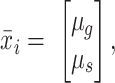where i is each class (nuclei vs. background) and µ_g and µ_s are the mean g and s phasor components, respectively. A within-class scatter matrix was then computed:

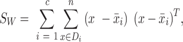where c is the number of classes (in this case 2) and D_i is the set of phasor values for each class i. The between-class scatter matrix was then computed:

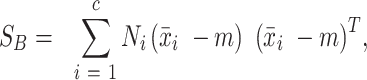where m is the mean of all classes and N_i is the number of pixels pertaining to each class i. The 1 x c matrix W was composed of the eigenvector with the highest eigenvalue as solved for the matrix:

The dot product between the phasor matrix for each image and W yielded the 1D transformed matrix:

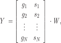where g are the g phasor values, s are the s phasor values, and N is the total number of pixels. Reshaping Y into the original 2D image shape yielded the LDA transformed image. This LDA image was then used as the “H” (hue) component, stacked with the fluorescence intensity and a “S” dummy matrix set at maximum value and transformed in color space into RGB.

Dense U-Net CNN for FLIM prediction from fluorescence intensity

K-means was used to segment the phasor images into K classes, representing pixels with similar phasor values (62). To employ the K-means algorithm, the phasor images for a given acquisition setting (i.e. 570/575 to 620 nm excitation/emission) were gathered, a background threshold value from the fluorescence intensity images was determined, and all phasor values corresponding to pixels above that threshold were pooled. The Scikit-Learn K-means algorithm was used to determine K cluster center values on the pooled data. Segmentations could then be generated for each image by determining the closest cluster center for each pixel using its g and s phasor values. These segmentations were used in combination with the background threshold to create “K + 1”-class segmentation masks for FLIM prediction.

An implementation of a dense U-Net CNN (46) was then used to predict these segmentation maps. The dense U-Net CNN, depicted in Fig. 3, is similar in architecture to the original U-Net CNN (70), but with added short skip connections at each layer. As with the original U-Net CNN (70), the architecture consists of four encoding layers, four decoding layers, and a bridge layer, employing two successive 3 × 3 kernel convolutions with ReLU activation at each layer. The encoding portion began with 64-feature channels, increasing 2-fold with each layer until a total of 1,024, while the decoding portion decreased feature channels two-fold back to the original 64. Max-pooling (2 × 2) and transposed convolutions (2 × 2) were used between layers for the encoding and decoding portions, respectively. The final convolutional block employed SoftMax activation to the “K + 1”-class mask.

For training, an official test set of five randomly selected, labeled/annotated images were set aside to be used for all experiments, except for cross-validation studies. Of the remaining seventy-five image sets, all or a random subset were randomly divided into training (80%) and validation (20%) sets. A patch size of 256 × 256 pixels from the input fluorescence intensity images (one or two channels) and output segmentation was used. Data augmentation consisted of random selection of the patch window, random flipping across the x and/or y axis, and random 0, 90, 180, or 270 degree rotation. A total loss consisting of the sum of the balanced, class-weighted dice loss and categorical focal loss (v1.0.1, https://github.com/qubvel/segmentation_models) was used for training with the Adam optimizer (base learning rate = 10⁻⁵, β₁ = 0.9, β₂ = 0.999, and ϵ = 10⁻⁸). Training was performed for 400 epochs with the model weights saved for the epoch with the lowest validation loss.

Cell instance segmentation and classification models

For all cell instance segmentation and cell classification studies, except when using cross-validation, the same randomly selected group of twelve training, three validation, and five testing image sets were used. Models were provided the RGB images as training input and cell-nuclei masks (instance segmentation) or class labels (classification) for output prediction. Additional model details are available in the Supplementary Material Appendix.

Cell instance segmentation was tested with three CNN architectures: Mask R-CNN (34, 35) with either a ResNet-50 or ResNet-101 backbone (https://github.com/matterport/Mask_RCNN) and Stardist (36) (https://github.com/stardist/stardist). Model weights were either initialized at random or from the model trained on fluorescence images of cell nuclei from the Data Science Bowl (DSB) 2018 dataset (7). The models were provided random 256 × 256 patches from the RGB images that were randomly rotated or flipped as input and the same patch of cell-nuclei masks as the ground-truth output for prediction. Training was performed over a total of 280 epochs (Mask R-CNN) or 400 epochs (Stardist) with the model weights saved for the epoch with the lowest validation loss.

Cell classification was tested with eight CNN architectures: DenseNet-121 (37), EfficientNetB5 (38), Inception-v3 (39), ResNet-50 and ResNet-101 (40), VGG16 and VGG19 (41), and Xception (42). Model weights were either initialized at random or from ImageNet (43). To generate images during training, cells were randomly selected and cropped (48 × 48) randomly within a ± 5 pixel x and y distance from the cell-nuclei center. These cropped images were further augmented by random flipping and rotation, and then resized to the input dimensions and preprocessed and normalized to the specifications of the CNN. Training was conducted over 100 epochs using the RMSprop optimizer and a learning rate of 2 × 10⁻⁶.

Cross-channel fluorescence and FLIM prediction

The same dense U-Net CNN design and parameters were implemented for cross-channel prediction of the fluorescence and FLIM data, except that the output was switched from a discrete prediction of K-means phasor classes to a continuous prediction of the fluorescence intensity and g- and s-phasor coordinates. This was accomplished by omitting the activation function in the final convolutional layer and using mean-squared error as the loss function.

Evaluation metrics

Further details of the evaluation metrics are available in the Supplementary Material Appendix.

Supplementary Material

pgac235_Supplemental_File

Click here for additional data file.^{(21.2MB, docx)}

ACKNOWLEDGEMENTS

We thank the Texas A&M Laboratory for Synthetic-Biologic Interactions (RRID: SCR_022287) and the Texas A&M Microscopy and Imaging Center (RRID: SCR_022128) for usage of instrumentation. We thank the Texas A&M Comparative Medicine Program for provision of mice and the Texas A&M Institute for Preclinical Studies for providing animal laboratory facilities.

Notes

Competing Interest: The authors declare no competing interest.

Contributor Information

Justin A Smolen, Departments of Chemistry, Chemical Engineering, and Materials Science and Engineering, Texas A&M University, College Station, TX 77842, USA.

Karen L Wooley, Departments of Chemistry, Chemical Engineering, and Materials Science and Engineering, Texas A&M University, College Station, TX 77842, USA.

Funding

The Welch Foundation is gratefully acknowledged for funding support through the W. T. Doherty-Welch Chair in Chemistry [Grant No. A-0001].

Authors' Contributions

Conception of work: J.A.S.

Data collection: J.A.S.

Data analysis and interpretation: J.A.S.

Drafting and revision of manuscript: J.A.S. and K.L.W.

Data Availability

The code to generate the RGB images from the source image data, to generate and train the dense U-Net CNN, and to train the cell classification models can be found on GitHub at https://github.com/jalexs82/flim_colorization. The datasets—including the FLIM images (Dataset S1), cell nuclei masks (Dataset S2), and the cell/tissue-type classification reference table (Dataset S3)—are available on Figshare (https://doi.org/10.6084/m9.figshare.21183517).

References

1. Gurcan MN, et al. 2009. Histopathological image analysis: a review. IEEE Rev Biomed Eng. 2:147–171. [DOI] [PMC free article] [PubMed] [Google Scholar]
2. Regev A, et al. 2018. The human cell atlas. eLife. 6:e27041. [DOI] [PMC free article] [PubMed] [Google Scholar]
3. Moen E, et al. 2019. Deep learning for cellular image analysis. Nat Methods. 16:1233–1246. [DOI] [PMC free article] [PubMed] [Google Scholar]
4. Durkee MS, Abraham R, Clark MR, Giger ML. 2021. Artificial intelligence and cellular segmentation in tissue microscopy images. Am J Pathol. 191:1693–1701. [DOI] [PMC free article] [PubMed] [Google Scholar]
5. LeCun Y, Bengio Y, Hinton G. 2015. Deep learning. Nature. 521:436–444. [DOI] [PubMed] [Google Scholar]
6. Greenwald NF, et al. 2021. Whole-cell segmentation of tissue images with human-level performance using large-scale data annotation and deep learning. Nat Biotechnol. 40(4): 555–565.. 10.1038/s41587-021-01094-0. [DOI] [PMC free article] [PubMed] [Google Scholar]
7. Caicedo JC, et al. 2019. Nucleus segmentation across imaging experiments: the 2018 Data Science Bowl. Nat Methods. 16(12):1247–1253. [DOI] [PMC free article] [PubMed] [Google Scholar]
8. Srinidhi CL, Ciga O, Martel AL. 2021. Deep neural network models for computational histopathology: a survey. Med Image Anal. 67:101813. [DOI] [PMC free article] [PubMed] [Google Scholar]
9. Bastiaens PIH, Squire A. 1999. Fluorescence lifetime imaging microscopy: spatial resolution of biochemical processes in the cell. Trends Cell Biol. 9(2): 48–52. [DOI] [PubMed] [Google Scholar]
10. Elangovan M, Day RN, Periasamy A. 2002. Nanosecond fluorescence resonance energy transfer-fluorescence lifetime imaging microscopy to localize the protein interactions in a single living cell. J Microsc. 205:3–14. [DOI] [PubMed] [Google Scholar]
11. Nothdurft R, Sarder P, Bloch S, Culver J, Achilefu S. 2012. Fluorescence lifetime imaging microscopy using near-infrared contrast agents. J Microsc. 247(2):202–207. [DOI] [PMC free article] [PubMed] [Google Scholar]
12. Grabolle M, et al. 2009. Fluorescence lifetime multiplexing with nanocrystals and organic labels. Anal Chem.81(18):7807–7813. [DOI] [PubMed] [Google Scholar]
13. Wu T-J, et al. 2013. Tracking the engraftment and regenerative capabilities of transplanted lung stem cells using fluorescent nanodiamonds. Nat Nanotechnol. 8:682–689. [DOI] [PMC free article] [PubMed] [Google Scholar]
14. del Rosal B, Benayas. A. 2018. Strategies to overcome autofluorescence In nanoprobe-driven in vivo fluorescence imaging. Small Methods. 2(9):1800075. [Google Scholar]
15. Jun YW, Kim HR, Reo YJ, Dai M, Ahn KH. 2017. Addressing the autofluorescence issue in deep tissue imaging by two-photon microscopy: the significance of far-red emitting dyes. Chem Sci. 8(11):7696–7704. [DOI] [PMC free article] [PubMed] [Google Scholar]
16. Vu T, et al. 2022. Spatial transcriptomics using combinatorial fluorescence spectral and lifetime encoding, imaging and analysis. Nat Commun. 13(1):169. [DOI] [PMC free article] [PubMed] [Google Scholar]
17. Lin H-J, Herman P, Lakowicz JR. 2003. Fluorescence lifetime-resolved pH imaging of living cells. Cytometry A. 52(2):77–89. [DOI] [PMC free article] [PubMed] [Google Scholar]
18. Kwiatek JM, et al. 2013. Characterization of a new series of fluorescent probes for imaging membrane order. PLoS One. 8(2):e52960. [DOI] [PMC free article] [PubMed] [Google Scholar]
19. Wang B, et al. 2015. Bipolar and fixable probe targeting mitochondria to trace local depolarization via two-photon fluorescence lifetime imaging. Analyst. 140:5488–5549. [DOI] [PubMed] [Google Scholar]
20. Levitt J, Chung P-H, Suhling K. 2015. Spectrally resolved fluorescence lifetime imaging of Nile red for measurements of intracellular polarity. J Biomedical Opt. 20:096002. [DOI] [PubMed] [Google Scholar]
21. Hille C, Lahn M, Löhmannsröben H-G, Dosche C. 2009. Two-photon fluorescence lifetime imaging of intracellular chloride in cockroach salivary glands. Photochem Photobiol Sci.8(3):319–327. [DOI] [PubMed] [Google Scholar]
22. Wilms CD, Eilers J. 2007. Photo-physical properties of Ca2+-indicator dyes suitable for two-photon fluorescence-lifetime recordings. J Microsc. 225:209–213. [DOI] [PubMed] [Google Scholar]
23. Despa S, Vecer J, Steels P, Ameloot M. 2000. Fluorescence lifetime microscopy of the Na+ indicator Sodium Green in HeLa cells. Anal Biochem. 281(2):159–175. [DOI] [PubMed] [Google Scholar]
24. Lee D-H, Li X, Ma N, Digman MA, Lee AP. 2018. Rapid and label-free identification of single leukemia cells from blood in a high-density microfluidic trapping array by fluorescence lifetime imaging microscopy. Lab Chip. 18(9):1349–1358. [DOI] [PubMed] [Google Scholar]
25. Chen B, et al. 2019. Support vector machine classification of nonmelanoma skin lesions based on fluorescence lifetime imaging microscopy. Anal Chem. 91(16):10640–10647. [DOI] [PubMed] [Google Scholar]
26. Tadrous PJ, et al. 2003. Fluorescence lifetime imaging of unstained tissues: early results in human breast cancer. J Pathol. 199(3):309–317. [DOI] [PubMed] [Google Scholar]
27. Yahav G, et al. 2016. Fluorescence lifetime imaging of DAPI-stained nuclei as a novel diagnostic tool for the detection and classification of B-cell chronic lymphocytic leukemia. Cytometry A. 89(7):644–652. [DOI] [PubMed] [Google Scholar]
28. Conklin MW, Provenzano PP, Eliceiri KW, Sullivan R, Keely PJ. 2009. Fluorescence lifetime imaging of endogenous fluorophores in histopathology sections reveals differences between normal and tumor epithelium in carcinoma in situ of the breast. Cell Biochem Biophys. 53(3):145–157. [DOI] [PMC free article] [PubMed] [Google Scholar]
29. Ranjit S, Malacrida L, Jameson DM, Gratton E. 2018. Fit-free analysis of fluorescence lifetime imaging data using the phasor approach. Nat Protoc. 13:1979–2004. [DOI] [PubMed] [Google Scholar]
30. Datta R, Heaster T, Sharick J, Gillette A, Skala M. 2020. Fluorescence lifetime imaging microscopy: fundamentals and advances in instrumentation, analysis, and applications. J Biomed Opt. 25:071203. [DOI] [PMC free article] [PubMed] [Google Scholar]
31. Wahl M, Orthaus-Müller S. 2014. Time tagged time-resolved fluorescence data collection in life sciences. Technical Note. PicoQuant GmbH, Germany. 2:1–10. [Google Scholar]
32. Jameson DM, Gratton E, Hall RD. 1984. The measurement and analysis of heterogeneous emissions by multifrequency phase and modulation fluorometry. Appl Spectrosc Rev. 20:55–106. [DOI] [PubMed] [Google Scholar]
33. Izenman AJ. 2013. Linear discriminant analysis. In: Casella G, Fienberg S, Olkin I. Modern multivariate statistical techniques. New York, NY. Springer. pp. 237–280. [Google Scholar]
34. He K, Gkioxari G, Dollár P, Girshick R. 2017. Mask r-cnn. In: Proceedings of the IEEE International Conference on Computer Vision. Venice, Italy. IEEE. 2961–2969. [Google Scholar]
35. Abdulla W. 2017. Mask r-cnn for object detection and instance segmentation on keras and tensorflow. [accessed 2021 Dec 6]. https://github.com/matterport/Mask_RCNN. [Google Scholar]
36. Schmidt U, Weigert M, Broaddus C, Myers G. 2018. Cell detection with star-convex polygons. In: Frangi A, Schnabel J, Davatzikos C, Alberola-López C, Fichtinger G. International Conference on Medical Image Computing and Computer-assisted Intervention. Grenada, Spain. Springer. pp. 265–273. [Google Scholar]
37. Huang G, Liu Z, Van Der Maaten L, Weinberger K Q. 2017. Densely connected convolutional networks. In: Proceedings of the IEEE Conference on Computer Vision and Pattern Recognition. Honolulu, HI. IEEE. pp. 4700–4708. [Google Scholar]
38. Tan M, Le Q. 2019. Efficientnet: rethinking model scaling for convolutional neural networks. In: Chaudhuri K, Salakhutdinov R. International Conference on Machine Learning. Long Beach, CA. PMLR. pp. 6105–6114. [Google Scholar]
39. Szegedy C, Vanhoucke V, Ioffe S, Shlens J, Wojna Z. 2016. Rethinking the inception architecture for computer vision. In: Proceedings of the IEEE Conference on Computer Vision and Pattern Recognition. Las Vegas, NV. IEEE. pp. 2818–2826. [Google Scholar]
40. He K, Zhang X, Ren S, Sun J. 2016. Deep residual learning for image recognition. In: Proceedings of the IEEE Conference on Computer Vision and Pattern Recognition. Las Vegas, NV. IEEE. pp. 770–778. [Google Scholar]
41. Simonyan K, Zisserman A. 2015. Very deep convolutional networks for large-scale image recognition. In: Bengio Y, LeCun Y. 3rd International Conference on Learning Representations. San Diego, CA. ICLR. [accessed 2022 Mar 21]. 10.48550/arXiv.1409.1556. [DOI] [Google Scholar]
42. Chollet F. 2017. Xception: deep learning with depthwise separable convolutions. In: Proceedings of the IEEE Conference on Computer Vision and Pattern Recognition. Honolulu, HI. IEEE. pp. 1251–1258. [Google Scholar]
43. Deng J, et al. 2009. ImageNet: a large-scale hierarchical image database. In: 2009 IEEE Conference on Computer Vision and Pattern Recognition. Miami FL. IEEE. 248–255. [Google Scholar]
44. ThermoFisher, Molecular Probes Fluorescence SpectraViewer. [accessed 2022 Mar 4]. http://thermofisher.com/spectraviewer. [Google Scholar]
45. McInnes L, Healy J, Melville J. 2018. Umap: uniform manifold approximation and projection for dimension reduction. arXiv. [accessed 2022 Mar 7]. 10.48550/arXiv.1802.03426. [DOI] [Google Scholar]
46. Kolařík M, Burget R, Uher V, Říha K, Dutta MK. 2019. Optimized high resolution 3D Dense-U-Net network for brain and spine segmentation. Appl Sci. 9:404. [Google Scholar]
47. Zhou W, Bovik AC, Sheikh HR, Simoncelli EP. 2004. Image quality assessment: from error visibility to structural similarity. IEEE Trans Image Process. 13:600–612. [DOI] [PubMed] [Google Scholar]
48. Maes F, Collignon A, Vandermeulen D, Marchal G, Suetens P. 1997. Multimodality image registration by maximization of mutual information. IEEE Trans Med Imaging. 16:187–198. [DOI] [PubMed] [Google Scholar]
49. Fienup J R. 1997. Invariant error metrics for image reconstruction. Appl Opt. 36:8352–8357. [DOI] [PubMed] [Google Scholar]
50. Silva E, Panetta K, Agaian S. 2007. Quantifying image similarity using measure of enhancement by entropy. In: Defense and Security Symposium. vol. 6579. Orlando, FL. SPIE. [Google Scholar]
51. Berisha S, et al. 2019. Deep learning for FTIR histology: leveraging spatial and spectral features with convolutional neural networks. Analyst. 144:1642–1653. [DOI] [PMC free article] [PubMed] [Google Scholar]
52. Zhang L, et al. 2019. Rapid histology of laryngeal squamous cell carcinoma with deep-learning based stimulated Raman scattering microscopy. Theranostics. 9(9):2541. [DOI] [PMC free article] [PubMed] [Google Scholar]
53. Beuque M, et al. 2021. Machine learning for grading and prognosis of esophageal dysplasia using mass spectrometry and histological imaging. Comput Biol Med. 138:104918. [DOI] [PubMed] [Google Scholar]
54. Betterle C, Zanchetta R. 2012. The immunofluorescence techniques in the diagnosis of endocrine autoimmune diseases. Auto Immun Highlights. 3(2):67–78. [DOI] [PMC free article] [PubMed] [Google Scholar]
55. Babu R A, et al. 2013. Immunofluorescence and its application in dermatopathology with oral manifestations: revisited. J Orofac Sci. 5(1):2. [Google Scholar]
56. Tan WCC, et al. 2020. Overview of multiplex immunohistochemistry/immunofluorescence techniques in the era of cancer immunotherapy. Cancer Commun. 40(4):135–153. [DOI] [PMC free article] [PubMed] [Google Scholar]
57. Rohilla S, Krämer B, Koberling F, Gregor I, Hocke AC. 2020. Multi-target immunofluorescence by separation of antibody cross-labelling via spectral-FLIM-FRET. Sci Rep. 10:3820. [DOI] [PMC free article] [PubMed] [Google Scholar]
58. Niehörster T, et al. 2016. Multi-target spectrally resolved fluorescence lifetime imaging microscopy. Nat Methods. 13(3):257–262. [DOI] [PubMed] [Google Scholar]
59. Stack EC, Wang C, Roman KA, Hoyt CC. 2014. Multiplexed immunohistochemistry, imaging, and quantitation: a review, with an assessment of Tyramide signal amplification, multispectral imaging and multiplex analysis. Methods. 70( 1):46–58. [DOI] [PubMed] [Google Scholar]
60. Mannam V, Zhang Y, Yuan X, Ravasio C, Howard SS. 2020. Machine learning for faster and smarter fluorescence lifetime imaging microscopy. J Phys Photonics. 2:042005. [Google Scholar]
61. Zhang R, Isola P, Efros AA. 2016. Colorful Image Colorization. Cham: Springer International Publishing, 649–666. [Google Scholar]
62. Zhang Y, et al. 2019. Automatic segmentation of intravital fluorescence microscopy images by K-means clustering of FLIM phasors. Opt Lett. 44(16):3928–3931. [DOI] [PubMed] [Google Scholar]
63. Guo J, Chen J, Lu C, Huang H. 2021. Medical image enhancement for lesion detection based on class-aware attention and deep colorization. In: 2021 IEEE 18th International Symposium on Biomedical Imaging (ISBI). Nice, France. IEEE. pp. 1746–1750. [Google Scholar]
64. Li B, Xie W. 2015. Adaptive fractional differential approach and its application to medical image enhancement. Comput Electr Eng. 45:324–335. [Google Scholar]
65. Escobar M, Castillo A, Romero A, Arbeláez P. 2020. UltraGAN: ultrasound enhancement through adversarial generation. In: Burgos N, Svoboda D, Wolterink J, Zhao C. International Workshop on Simulation and Synthesis in Medical Imaging. Lima, Peru: Springer-Verlag. pp. 120–130. [Google Scholar]
66. Teare P, Fishman M, Benzaquen O, Toledano E, Elnekave E. 2017. Malignancy detection on mammography using dual deep convolutional neural networks and genetically discovered false color input enhancement. J Digit Imaging. 30:499–505. [DOI] [PMC free article] [PubMed] [Google Scholar]
67. Morra L, Piano L, Lamberti F, Tommasi T. 2021. Bridging the gap between Natural and Medical Images through Deep Colorization. In: 2020 25th International Conference on Pattern Recognition (ICPR). Milan, Italy. IEEE. pp. 835–842. [Google Scholar]
68. Wold S, Esbensen K, Geladi P. 1987. Principal component analysis. Chemometr Intell Lab Syst.2:37–52. [Google Scholar]
69. Arzt M, et al. 2022. LABKIT: labeling and segmentation toolkit for big image data. Front Comput Sci. 4:777728. [Google Scholar]
70. Ronneberger O, Fischer P, Brox T.. 2015.; U-net: Convolutional networks for biomedical image segmentation. In: Navab N, Hornegger J, Wells W, Frangi A. International Conference on Medical Image Computing and Computer-assisted Intervention. Munich, Germany. Springer. pp. 234–241. [Google Scholar]

Associated Data

This section collects any data citations, data availability statements, or supplementary materials included in this article.

Supplementary Materials

pgac235_Supplemental_File

Click here for additional data file.^{(21.2MB, docx)}

Data Availability Statement

[bib1] 1. Gurcan MN, et al. 2009. Histopathological image analysis: a review. IEEE Rev Biomed Eng. 2:147–171. [DOI] [PMC free article] [PubMed] [Google Scholar]

[bib2] 2. Regev A, et al. 2018. The human cell atlas. eLife. 6:e27041. [DOI] [PMC free article] [PubMed] [Google Scholar]

[bib3] 3. Moen E, et al. 2019. Deep learning for cellular image analysis. Nat Methods. 16:1233–1246. [DOI] [PMC free article] [PubMed] [Google Scholar]

[bib4] 4. Durkee MS, Abraham R, Clark MR, Giger ML. 2021. Artificial intelligence and cellular segmentation in tissue microscopy images. Am J Pathol. 191:1693–1701. [DOI] [PMC free article] [PubMed] [Google Scholar]

[bib5] 5. LeCun Y, Bengio Y, Hinton G. 2015. Deep learning. Nature. 521:436–444. [DOI] [PubMed] [Google Scholar]

[bib6] 6. Greenwald NF, et al. 2021. Whole-cell segmentation of tissue images with human-level performance using large-scale data annotation and deep learning. Nat Biotechnol. 40(4): 555–565.. 10.1038/s41587-021-01094-0. [DOI] [PMC free article] [PubMed] [Google Scholar]

[bib7] 7. Caicedo JC, et al. 2019. Nucleus segmentation across imaging experiments: the 2018 Data Science Bowl. Nat Methods. 16(12):1247–1253. [DOI] [PMC free article] [PubMed] [Google Scholar]

[bib8] 8. Srinidhi CL, Ciga O, Martel AL. 2021. Deep neural network models for computational histopathology: a survey. Med Image Anal. 67:101813. [DOI] [PMC free article] [PubMed] [Google Scholar]

[bib9] 9. Bastiaens PIH, Squire A. 1999. Fluorescence lifetime imaging microscopy: spatial resolution of biochemical processes in the cell. Trends Cell Biol. 9(2): 48–52. [DOI] [PubMed] [Google Scholar]

[bib10] 10. Elangovan M, Day RN, Periasamy A. 2002. Nanosecond fluorescence resonance energy transfer-fluorescence lifetime imaging microscopy to localize the protein interactions in a single living cell. J Microsc. 205:3–14. [DOI] [PubMed] [Google Scholar]

[bib11] 11. Nothdurft R, Sarder P, Bloch S, Culver J, Achilefu S. 2012. Fluorescence lifetime imaging microscopy using near-infrared contrast agents. J Microsc. 247(2):202–207. [DOI] [PMC free article] [PubMed] [Google Scholar]

[bib12] 12. Grabolle M, et al. 2009. Fluorescence lifetime multiplexing with nanocrystals and organic labels. Anal Chem.81(18):7807–7813. [DOI] [PubMed] [Google Scholar]

[bib13] 13. Wu T-J, et al. 2013. Tracking the engraftment and regenerative capabilities of transplanted lung stem cells using fluorescent nanodiamonds. Nat Nanotechnol. 8:682–689. [DOI] [PMC free article] [PubMed] [Google Scholar]

[bib14] 14. del Rosal B, Benayas. A. 2018. Strategies to overcome autofluorescence In nanoprobe-driven in vivo fluorescence imaging. Small Methods. 2(9):1800075. [Google Scholar]

[bib15] 15. Jun YW, Kim HR, Reo YJ, Dai M, Ahn KH. 2017. Addressing the autofluorescence issue in deep tissue imaging by two-photon microscopy: the significance of far-red emitting dyes. Chem Sci. 8(11):7696–7704. [DOI] [PMC free article] [PubMed] [Google Scholar]

[bib16] 16. Vu T, et al. 2022. Spatial transcriptomics using combinatorial fluorescence spectral and lifetime encoding, imaging and analysis. Nat Commun. 13(1):169. [DOI] [PMC free article] [PubMed] [Google Scholar]

[bib17] 17. Lin H-J, Herman P, Lakowicz JR. 2003. Fluorescence lifetime-resolved pH imaging of living cells. Cytometry A. 52(2):77–89. [DOI] [PMC free article] [PubMed] [Google Scholar]

[bib18] 18. Kwiatek JM, et al. 2013. Characterization of a new series of fluorescent probes for imaging membrane order. PLoS One. 8(2):e52960. [DOI] [PMC free article] [PubMed] [Google Scholar]

[bib19] 19. Wang B, et al. 2015. Bipolar and fixable probe targeting mitochondria to trace local depolarization via two-photon fluorescence lifetime imaging. Analyst. 140:5488–5549. [DOI] [PubMed] [Google Scholar]

[bib20] 20. Levitt J, Chung P-H, Suhling K. 2015. Spectrally resolved fluorescence lifetime imaging of Nile red for measurements of intracellular polarity. J Biomedical Opt. 20:096002. [DOI] [PubMed] [Google Scholar]

[bib21] 21. Hille C, Lahn M, Löhmannsröben H-G, Dosche C. 2009. Two-photon fluorescence lifetime imaging of intracellular chloride in cockroach salivary glands. Photochem Photobiol Sci.8(3):319–327. [DOI] [PubMed] [Google Scholar]

[bib22] 22. Wilms CD, Eilers J. 2007. Photo-physical properties of Ca2+-indicator dyes suitable for two-photon fluorescence-lifetime recordings. J Microsc. 225:209–213. [DOI] [PubMed] [Google Scholar]

[bib23] 23. Despa S, Vecer J, Steels P, Ameloot M. 2000. Fluorescence lifetime microscopy of the Na+ indicator Sodium Green in HeLa cells. Anal Biochem. 281(2):159–175. [DOI] [PubMed] [Google Scholar]

[bib24] 24. Lee D-H, Li X, Ma N, Digman MA, Lee AP. 2018. Rapid and label-free identification of single leukemia cells from blood in a high-density microfluidic trapping array by fluorescence lifetime imaging microscopy. Lab Chip. 18(9):1349–1358. [DOI] [PubMed] [Google Scholar]

[bib25] 25. Chen B, et al. 2019. Support vector machine classification of nonmelanoma skin lesions based on fluorescence lifetime imaging microscopy. Anal Chem. 91(16):10640–10647. [DOI] [PubMed] [Google Scholar]

[bib26] 26. Tadrous PJ, et al. 2003. Fluorescence lifetime imaging of unstained tissues: early results in human breast cancer. J Pathol. 199(3):309–317. [DOI] [PubMed] [Google Scholar]

[bib27] 27. Yahav G, et al. 2016. Fluorescence lifetime imaging of DAPI-stained nuclei as a novel diagnostic tool for the detection and classification of B-cell chronic lymphocytic leukemia. Cytometry A. 89(7):644–652. [DOI] [PubMed] [Google Scholar]

[bib28] 28. Conklin MW, Provenzano PP, Eliceiri KW, Sullivan R, Keely PJ. 2009. Fluorescence lifetime imaging of endogenous fluorophores in histopathology sections reveals differences between normal and tumor epithelium in carcinoma in situ of the breast. Cell Biochem Biophys. 53(3):145–157. [DOI] [PMC free article] [PubMed] [Google Scholar]

[bib29] 29. Ranjit S, Malacrida L, Jameson DM, Gratton E. 2018. Fit-free analysis of fluorescence lifetime imaging data using the phasor approach. Nat Protoc. 13:1979–2004. [DOI] [PubMed] [Google Scholar]

[bib30] 30. Datta R, Heaster T, Sharick J, Gillette A, Skala M. 2020. Fluorescence lifetime imaging microscopy: fundamentals and advances in instrumentation, analysis, and applications. J Biomed Opt. 25:071203. [DOI] [PMC free article] [PubMed] [Google Scholar]

[bib31] 31. Wahl M, Orthaus-Müller S. 2014. Time tagged time-resolved fluorescence data collection in life sciences. Technical Note. PicoQuant GmbH, Germany. 2:1–10. [Google Scholar]

[bib32] 32. Jameson DM, Gratton E, Hall RD. 1984. The measurement and analysis of heterogeneous emissions by multifrequency phase and modulation fluorometry. Appl Spectrosc Rev. 20:55–106. [DOI] [PubMed] [Google Scholar]

[bib33] 33. Izenman AJ. 2013. Linear discriminant analysis. In: Casella G, Fienberg S, Olkin I. Modern multivariate statistical techniques. New York, NY. Springer. pp. 237–280. [Google Scholar]

[bib34] 34. He K, Gkioxari G, Dollár P, Girshick R. 2017. Mask r-cnn. In: Proceedings of the IEEE International Conference on Computer Vision. Venice, Italy. IEEE. 2961–2969. [Google Scholar]

[bib35] 35. Abdulla W. 2017. Mask r-cnn for object detection and instance segmentation on keras and tensorflow. [accessed 2021 Dec 6]. https://github.com/matterport/Mask_RCNN. [Google Scholar]

[bib36] 36. Schmidt U, Weigert M, Broaddus C, Myers G. 2018. Cell detection with star-convex polygons. In: Frangi A, Schnabel J, Davatzikos C, Alberola-López C, Fichtinger G. International Conference on Medical Image Computing and Computer-assisted Intervention. Grenada, Spain. Springer. pp. 265–273. [Google Scholar]

[bib37] 37. Huang G, Liu Z, Van Der Maaten L, Weinberger K Q. 2017. Densely connected convolutional networks. In: Proceedings of the IEEE Conference on Computer Vision and Pattern Recognition. Honolulu, HI. IEEE. pp. 4700–4708. [Google Scholar]

[bib38] 38. Tan M, Le Q. 2019. Efficientnet: rethinking model scaling for convolutional neural networks. In: Chaudhuri K, Salakhutdinov R. International Conference on Machine Learning. Long Beach, CA. PMLR. pp. 6105–6114. [Google Scholar]

[bib39] 39. Szegedy C, Vanhoucke V, Ioffe S, Shlens J, Wojna Z. 2016. Rethinking the inception architecture for computer vision. In: Proceedings of the IEEE Conference on Computer Vision and Pattern Recognition. Las Vegas, NV. IEEE. pp. 2818–2826. [Google Scholar]

[bib40] 40. He K, Zhang X, Ren S, Sun J. 2016. Deep residual learning for image recognition. In: Proceedings of the IEEE Conference on Computer Vision and Pattern Recognition. Las Vegas, NV. IEEE. pp. 770–778. [Google Scholar]

[bib41] 41. Simonyan K, Zisserman A. 2015. Very deep convolutional networks for large-scale image recognition. In: Bengio Y, LeCun Y. 3rd International Conference on Learning Representations. San Diego, CA. ICLR. [accessed 2022 Mar 21]. 10.48550/arXiv.1409.1556. [DOI] [Google Scholar]

[bib42] 42. Chollet F. 2017. Xception: deep learning with depthwise separable convolutions. In: Proceedings of the IEEE Conference on Computer Vision and Pattern Recognition. Honolulu, HI. IEEE. pp. 1251–1258. [Google Scholar]

[bib43] 43. Deng J, et al. 2009. ImageNet: a large-scale hierarchical image database. In: 2009 IEEE Conference on Computer Vision and Pattern Recognition. Miami FL. IEEE. 248–255. [Google Scholar]

[bib44] 44. ThermoFisher, Molecular Probes Fluorescence SpectraViewer. [accessed 2022 Mar 4]. http://thermofisher.com/spectraviewer. [Google Scholar]

[bib45] 45. McInnes L, Healy J, Melville J. 2018. Umap: uniform manifold approximation and projection for dimension reduction. arXiv. [accessed 2022 Mar 7]. 10.48550/arXiv.1802.03426. [DOI] [Google Scholar]

[bib46] 46. Kolařík M, Burget R, Uher V, Říha K, Dutta MK. 2019. Optimized high resolution 3D Dense-U-Net network for brain and spine segmentation. Appl Sci. 9:404. [Google Scholar]

[bib47] 47. Zhou W, Bovik AC, Sheikh HR, Simoncelli EP. 2004. Image quality assessment: from error visibility to structural similarity. IEEE Trans Image Process. 13:600–612. [DOI] [PubMed] [Google Scholar]

[bib48] 48. Maes F, Collignon A, Vandermeulen D, Marchal G, Suetens P. 1997. Multimodality image registration by maximization of mutual information. IEEE Trans Med Imaging. 16:187–198. [DOI] [PubMed] [Google Scholar]

[bib49] 49. Fienup J R. 1997. Invariant error metrics for image reconstruction. Appl Opt. 36:8352–8357. [DOI] [PubMed] [Google Scholar]

[bib50] 50. Silva E, Panetta K, Agaian S. 2007. Quantifying image similarity using measure of enhancement by entropy. In: Defense and Security Symposium. vol. 6579. Orlando, FL. SPIE. [Google Scholar]

[bib51] 51. Berisha S, et al. 2019. Deep learning for FTIR histology: leveraging spatial and spectral features with convolutional neural networks. Analyst. 144:1642–1653. [DOI] [PMC free article] [PubMed] [Google Scholar]

[bib52] 52. Zhang L, et al. 2019. Rapid histology of laryngeal squamous cell carcinoma with deep-learning based stimulated Raman scattering microscopy. Theranostics. 9(9):2541. [DOI] [PMC free article] [PubMed] [Google Scholar]

[bib53] 53. Beuque M, et al. 2021. Machine learning for grading and prognosis of esophageal dysplasia using mass spectrometry and histological imaging. Comput Biol Med. 138:104918. [DOI] [PubMed] [Google Scholar]

[bib54] 54. Betterle C, Zanchetta R. 2012. The immunofluorescence techniques in the diagnosis of endocrine autoimmune diseases. Auto Immun Highlights. 3(2):67–78. [DOI] [PMC free article] [PubMed] [Google Scholar]

[bib55] 55. Babu R A, et al. 2013. Immunofluorescence and its application in dermatopathology with oral manifestations: revisited. J Orofac Sci. 5(1):2. [Google Scholar]

[bib56] 56. Tan WCC, et al. 2020. Overview of multiplex immunohistochemistry/immunofluorescence techniques in the era of cancer immunotherapy. Cancer Commun. 40(4):135–153. [DOI] [PMC free article] [PubMed] [Google Scholar]

[bib57] 57. Rohilla S, Krämer B, Koberling F, Gregor I, Hocke AC. 2020. Multi-target immunofluorescence by separation of antibody cross-labelling via spectral-FLIM-FRET. Sci Rep. 10:3820. [DOI] [PMC free article] [PubMed] [Google Scholar]

[bib58] 58. Niehörster T, et al. 2016. Multi-target spectrally resolved fluorescence lifetime imaging microscopy. Nat Methods. 13(3):257–262. [DOI] [PubMed] [Google Scholar]

[bib59] 59. Stack EC, Wang C, Roman KA, Hoyt CC. 2014. Multiplexed immunohistochemistry, imaging, and quantitation: a review, with an assessment of Tyramide signal amplification, multispectral imaging and multiplex analysis. Methods. 70( 1):46–58. [DOI] [PubMed] [Google Scholar]

[bib60] 60. Mannam V, Zhang Y, Yuan X, Ravasio C, Howard SS. 2020. Machine learning for faster and smarter fluorescence lifetime imaging microscopy. J Phys Photonics. 2:042005. [Google Scholar]

[bib61] 61. Zhang R, Isola P, Efros AA. 2016. Colorful Image Colorization. Cham: Springer International Publishing, 649–666. [Google Scholar]

[bib62] 62. Zhang Y, et al. 2019. Automatic segmentation of intravital fluorescence microscopy images by K-means clustering of FLIM phasors. Opt Lett. 44(16):3928–3931. [DOI] [PubMed] [Google Scholar]

[bib63] 63. Guo J, Chen J, Lu C, Huang H. 2021. Medical image enhancement for lesion detection based on class-aware attention and deep colorization. In: 2021 IEEE 18th International Symposium on Biomedical Imaging (ISBI). Nice, France. IEEE. pp. 1746–1750. [Google Scholar]

[bib64] 64. Li B, Xie W. 2015. Adaptive fractional differential approach and its application to medical image enhancement. Comput Electr Eng. 45:324–335. [Google Scholar]

[bib65] 65. Escobar M, Castillo A, Romero A, Arbeláez P. 2020. UltraGAN: ultrasound enhancement through adversarial generation. In: Burgos N, Svoboda D, Wolterink J, Zhao C. International Workshop on Simulation and Synthesis in Medical Imaging. Lima, Peru: Springer-Verlag. pp. 120–130. [Google Scholar]

[bib66] 66. Teare P, Fishman M, Benzaquen O, Toledano E, Elnekave E. 2017. Malignancy detection on mammography using dual deep convolutional neural networks and genetically discovered false color input enhancement. J Digit Imaging. 30:499–505. [DOI] [PMC free article] [PubMed] [Google Scholar]

[bib67] 67. Morra L, Piano L, Lamberti F, Tommasi T. 2021. Bridging the gap between Natural and Medical Images through Deep Colorization. In: 2020 25th International Conference on Pattern Recognition (ICPR). Milan, Italy. IEEE. pp. 835–842. [Google Scholar]

[bib68] 68. Wold S, Esbensen K, Geladi P. 1987. Principal component analysis. Chemometr Intell Lab Syst.2:37–52. [Google Scholar]

[bib69] 69. Arzt M, et al. 2022. LABKIT: labeling and segmentation toolkit for big image data. Front Comput Sci. 4:777728. [Google Scholar]

[bib70] 70. Ronneberger O, Fischer P, Brox T.. 2015.; U-net: Convolutional networks for biomedical image segmentation. In: Navab N, Hornegger J, Wells W, Frangi A. International Conference on Medical Image Computing and Computer-assisted Intervention. Munich, Germany. Springer. pp. 234–241. [Google Scholar]

PERMALINK

Fluorescence lifetime image microscopy prediction with convolutional neural networks for cell detection and classification in tissues

Justin A Smolen

Karen L Wooley

Roles

Abstract

Significance Statement.

Introduction

Results

Fig. 1.

Comparison of FLIM and fluorescence images for cell detection and classification

Fig. 2.

Generation of FLIM images via a dense U-Net CNN using fluorescence image data

Fig. 3.

Generated FLIM images enhance cell-nuclei instance segmentation and cell/tissue classification over fluorescence intensity alone

Fig. 4.

Fig. 5.

FLIM data provides high accuracy in cross-channel prediction

Fig. 6.

Discussion

FLIM and machine learning

Materials and Methods

Tissue preparation and imaging

Software and hardware

Image data annotation and processing

Dense U-Net CNN for FLIM prediction from fluorescence intensity

Cell instance segmentation and classification models

Cross-channel fluorescence and FLIM prediction

Evaluation metrics

Supplementary Material

ACKNOWLEDGEMENTS

Notes

Contributor Information

Funding

Authors' Contributions

Data Availability

References

Associated Data

Supplementary Materials

Data Availability Statement

ACTIONS

PERMALINK

RESOURCES

Similar articles

Cited by other articles

Links to NCBI Databases