Abstract
Dealing with the ill-posed and non-unique nature of the non-linear geophysical inverse problem via local optimizers requires the use of some regularization methods, constraints, and prior information about the Earth's complex interior. Another difficulty is that the success of local search algorithms depends on a well-designed initial model located close to the parameter set providing the global minimum. On the other hand, global optimization and metaheuristic algorithms that have the ability to scan almost the entire model space do not need an assertive initial model. Thus, these approaches are increasingly incorporated into parameter estimation studies and are also gaining more popularity in the geophysical community. In this study we present the Barnacles Mating Optimizer (BMO), a recently proposed global optimizer motivated by the special mating behavior of barnacles, to interpret magnetic anomalies. This is the first example in the literature of BMO application to a geophysical inverse problem. After performing modal analyses and parameter tuning processes, BMO has been tested on simulated magnetic anomalies generated from hypothetical models and subsequently applied to three real anomalies that are chromite deposit, uranium deposit and Mesozoic dike. A second moving average (SMA) scheme to eliminate regional anomalies from observed anomalies has been examined and certified. Post-inversion uncertainty assessment analyses have been also implemented to understand the reliability of the solutions achieved. Moreover, BMO’s solutions for convergence rate, stability, robustness and accuracy have been compared with the solutions of the commonly used standard Particle Swarm Optimization (sPSO) algorithm. The results have shown that the BMO algorithm can scan the model parameter space more extensively without affecting its ability to consistently approach the unique global minimum in this presented inverse problem. We, therefore, recommend the use of competitive BMO in model parameter estimation studies performed with other geophysical methods.
Subject terms: Environmental sciences, Solid Earth sciences
Introduction
The magnetic method has so far been used in a wide range of investigations at various sites1–11. The most important task of the magnetic method is to explore subsurface geology using minor changes in the geomagnetic field caused by magnetized masses. As with other geophysical methods, magnetic anomalies are assessed by making some assumptions and generalizations. Magnetized masses are commonly analyzed using some simple-shaped source structures12,13. However, these geometrically idealized source structures cannot be considered geologically perfect, but are used in the investigation of the magnetic anomalies to simplify modelling and interpretation procedures14–17. In order to better interpret magnetized causative structures, many computational approaches have been proposed, such as matching curve18,19, Fourier and Hilbert Transforms20, characteristics points and distances21, Least-squares approximations22–24, Euler Deconvolution25, simplex algorithm26, correlation techniques27, variance analyses28, derivative-based and moving average-based algorithms29,30, spectral analysis techniques31, and local wave number techniques32. In addition to these methodologies, the most frequently used tool for interpreting magnetic anomalies is the inversion approach. In geophysics, reconstructing the appropriate subsurface model using a set of observations is known as inversion or inverse problem. Owing to the well-acknowledged ill-posed and non-unique nature of magnetic inverse problems, estimations of the model parameters of buried magnetized sources can be achieved through some challenging processes33–37. Local and global search algorithms can be applied for the inversion procedure21,38. Derivative-based local search algorithms using various regularization procedures have been routinely used for this task. Despite their very fast convergence characteristics, they have some serious disadvantages. These algorithms require prior information depending on geological conditions. Moreover, their success largely depends on the choice of initial guess and therefore they cannot scan the entire model space. They typically tend to reach a minimum in the vicinity of the initial model parameter set. Thus, these optimizers may reach any local minimum instead of the global minimum which is the deepest valley in the objective function surface topography. On the other hand, derivative-free global optimization and metaheuristic algorithms use a random walk search to reach the minimum in the given model parameter space. They can effectively scan the entire model space and therefore do not require a well-designed initial guess. Additionally, they have the ability of escaping local minima in the complex nature of the error function topography. Because of these advantages, the use of such nature-inspired algorithms in geophysical inverse problems has become very popular over the last decade. In fact, the first applications of these intelligence algorithms date back to the years before 1940, which is called the pre-theoretical period when the studies were informal39. The period between 1940 and 1980 is the early period, and these algorithms were formally studied during this period. In the method-centric period which is between 1980 and 2000 metaheuristic studies increased dramatically and numerous different approaches were introduced as an alternative tool to classical optimization algorithms40. The period from the 2000s to the present is called the framework-centric period, and the idea of describing computational intelligence algorithms as frameworks rather than methods has increased39.
Standard Particle Swarm Optimization (sPSO) and Genetic Algorithm (GA) are commonly used in geophysical inversion41. Some comparative studies have verified that sPSO outperforms GA in terms of accurateness and better convergence characteristics for various problems42–45. However, it should be noted that there is no optimal metaheuristic algorithm for solving all types of inverse problems. Therefore, new problem-specific global optimization algorithms are still being developed. Accordingly, adaptations of new nature-inspired derivative-free algorithms for the inversion of magnetic anomalies have taken their place in the literature. In most cases, the outputs obtained were not compared with the results of another metaheuristic algorithm. Besides, in most studies, possible uncertainties in the model parameters obtained were not investigated. However, it is a well-known fact that global optimization and metaheuristic algorithms allow to perform uncertainty analysis which is an essential step in understanding the reliability of the solutions obtained. The difficulty of the inverse problem is increased when multiple-source structures are used to represent the resulting magnetic anomalies. Therefore, some of the anomaly peaks are not used in most studies, and the number of source structures is reduced and attempts are made to find a solution. In addition, it is an important deficiency that the possible regional magnetic anomaly effect is mostly ignored. Table 1 lists information about magnetic anomaly inversion studies carried out in recent years with global optimization algorithms and the presented study. It is clear that comparative tests, uncertainty analyses and regional effect investigations were not performed together in previous studies. In this study, we present a novel bio-inspired algorithm called Barnacles Mating Optimizer (BMO) for the inversion of magnetic anomalies. This optimization algorithm imitates the unique mating character of barnacles. Three theoretical cases with different scenarios were used to understand the proficiency of the proposed algorithm. Besides, three real data sets, including a chromite ore anomaly (India), an uranium ore anomaly (India) and an intrusive Mesozoic dyke anomaly (Brazil) were taken into consideration. Prior to the inversion experiments, we performed some modal analyses by mapping the surface topographies of the objective function for the model parameter pairs. Thuswise the resolvabilities of model parameters and their effects on objective function were explored. Following the previous works9,46 we also investigated the regional background effect through the second moving average (SMA) technique. Consistency and credibility of the solutions obtained were assessed by performing some uncertainty appraisal analyses. Finally, the performances of the BMO and sPSO algorithms in our case were compared.
Table 1.
Magnetic anomaly inversion studies carried out in recent years with global optimization algorithms and the presented study.
| Algorithm | Inspiration | Compared with | Uncertainty analyses | Regional analyses | Magnetic anomaly |
|---|---|---|---|---|---|
| Ant-Colony Optimization (ACO)47 | Strategies of ant colonies to find the shortest path | PSO | No | No | Six sources |
| Simulated Annealing Optimization (SAO)34 | Metal annealing process | None | Yes | No | Single source |
| Genetic Algorithm (GA)48 | Evolutionary procedures | None | No | No | Single source |
| Differential Evolution Algorithm (DEA)49 | Evolutionary procedures | None | No | No | Two sources |
| Grey Wolf Optimization (GWO)50 | Hierarchical behaviors of grey wolves for hunting | PSO | No | No | Four sources |
| Particle Swarm Optimization (PSO)51 | Behaviors of foraging birds and fish | None | No | No | Two sources |
| Genetic Price Algorithm (GPA)52 | Genetic random search procedure | None | No | No | Three sources |
| Whale Optimization (WO)53 | Strategies of humpback whales seeking prey | None | No | No | Single source |
| Differential Search Algorithm (DSA)54 | Superorganism migrations | None | Yes | No | Two sources |
| Adaptive Differential Evolution (ADE)55 | Evolutionary procedures | None | No | No | Two sources |
| Bat Algorithm Optimization (BAO)56 | Echolocation behaviors of microbats | None | No | No | Two sources |
| Manta-Ray Foraging Optimization (MFO)57 | Intelligent behaviors of manta-rays | PSO, SA, GA | No | No | Two sources |
| Social Spider Optimization (SSO)58 | Foraging strategies of social spiders | None | Yes | No | Two sources |
| Hybrid PSO-GA59 | Behaviors of foraging birds and fish with genetic operators | None | No | No | Single source |
| Barnacles Mating Optimizer (BMO) | Mating behavior of barnacles | PSO | Yes | Yes | Four sources |
Methodology
Forward modeling
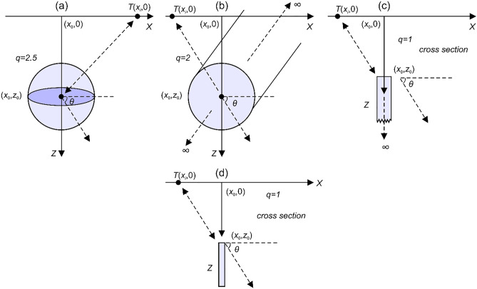
The magnetic anomaly equations for some idealized sources (Fig. 1) such as a sphere60,61, an infinitely long horizontal cylinder62, a thin dyke23,63,64 and a thin sheet63 are given below, respectively.
| 1 |
| 2 |
| 3 |
| 4 |
Figure 1.
Illustrations of geometries and parameters of (a) a sphere, (b) an infinitely long horizontal cylinder, (c) a thin dyke, and (d) a thin sheet.
In the definitions given above, T is the total field magnetic anomaly, xi is the observation point on a profile, z0 (m) represents the depth to the center of the buried magnetic source (spheres and cylinders) and the top of dykes and thin sheets, θ denotes the effective magnetization angle (degree), q represents the shape factor (dimensionless), x0 defines the origin of the anomaly or the horizontal center coordinate of the magnetic source (m), and K denotes the coefficient of amplitude (nT × m2q−2), which is related to the model shape. The shape factors 2.5, 2, 1, and 1 are used for spheres, horizontal cylinders, thin dykes, and thin sheets, respectively12. On the basis of principle of superposition, composite magnetic anomalies of multiple-source are calculated easily using the following definition12.
| 5 |
where Tj and P are the magnetic anomaly of j-th source and the number of sources, respectively.
Undesired regional effect and local interruption
It is well-acknowledged that, due to the heterogeneity of the Earth’s interior, the measured residual magnetic anomaly of a certain shallow source is mostly corrupted by undesired regional effects and some local interferences. The mathematical definitions of these effects are given as follows9:
| 6 |
where Tgen(xi) denotes the composite anomaly, Tre(xi) is the undesired regional effect (c0–c3 are predefined constants), and Tlocal(xi) represents the local perturbations originated from interfering sources.
SMA method
A residual magnetic response of a shallow source can be calculated by removing the regional effect from the observed data set. A recent study9 reported the efficiency of the SMA method to achieve this goal using the following definition:
| 7 |
where R2(x) is the approximated residual magnetic anomaly, and s (m) denotes the window length. Typically, in order to provide a reasonable estimate of the true model parameters we can simply use the mean output produced by delimiting the SMA magnetic anomalies, which is controlled by s values (window length).
BMO
BMO is a novel algorithm65, which is used to simulate the special mating behaviors of barnacles for the optimization of some engineering problems. Barnacles are mostly hermaphrodites and live in shallow and tidal waters. These fantastic individuals can attach themselves temporarily to substratum or symbionts in the water. For this purpose, they mostly use whales, sea snakes or any other crustaceans. In order to survive, barnacle mating groups surround neighbors and potential competitors within reach of their penises.
The reported65 satisfactory results of BMO in 23 challenging benchmark functions and power system analyses motivated us to apply it to nonlinear geophysical problems. Applications with many different scenarios are presented to show how the proposed algorithm can reach the global optimum without suffering from the local optima entrapments and without being affected by the ill-posed nature of the magnetic inverse problem. The steps of the algorithm are given in brief as follows.
Initialization
In BMO, it is assumed that barnacles are the solutions65. Thus, in the inverse problem presented here barnacles can be treated as the model parameters (K, θ, x0, z0, q). The matrix of population X is defined as follows:
| 8 |
where dim is the number of control variables (dim = 5 in this study) and N denotes the number of barnacles (population size). The (the i-th control variable of the j-th barnacle. Here, i = 1, 2, 3... dim, j = 1, 2, 3... N) given above is subject to the upper and lower bounds [lbi, ubi]. The appraisal of X is terminated primarily, and the sorting process based on the obtained fitness values is carried out to detect the best solution (K, θ, x0, z0, q) at the top of X.
Selection process
BMO uses a different system compared to other evolution-based systems such as Genetic algorithm66, Differential Evolution67 etc. As the selection of two barnacles is relied on the length of their penises (pl) a simple case can be presented65 to illustrate this special mating behavior assuming that the best solution is located at the top of X at a particular iteration and the maximum penis length of barnacles pl = 7. Therefore, barnacle #1 is only able to mate with one of barnacles #2 and #7 (selected barnacles are located within pl). Hence, the following simple mathematical forms to achieve the selection process is proposed65:
| 9 |
where randperm(N) is a function that returns a row vector that contains a random permutation of the integers from 1 to N inclusive. The barnacled and barnaclem are the parents to be mated and they should locate within pl. However, if one of them does not fulfill this requirement, the normal mating process is therefore postponed. The next generation is updated using the sperm casting process instead.
Reproduction
BMO’s reproduction progression differs from other evolution-based algorithms. There is no explicit formula for developing the reproduction of barnacles, so BMO produces offspring based on the principle of the Hardy–Weinberg68,69. The following expression is given for this procedure:
| 10 |
where p represents random numbers in the range of [0, 1], q = (1 − p), and are selected parents using Eq. (9). p and q denote the percentage of characteristics of the mating objects implanted in the next generation. The offspring, therefore, inherits the behaviors depending on the probability of the random number in the range of [0, 1].
In the BMO algorithm pl has an important impact on the exploitation (normal mating process) and exploration stages. The exploitation process occurs if the selected barnacle to be mated is within the penis length of the male barnacle. If not, the sperm cast is implemented and considered as an exploration process of BMO as given below:
| 11 |
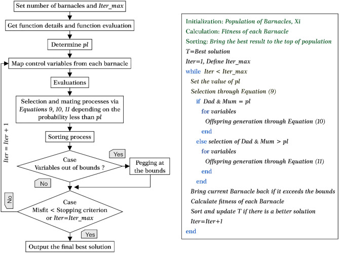
where rand() denotes random numbers between [0, 1]. Along with Eq. (11), the new offspring is formed by the female barnacle because the female barnacle retrieves the sperm from the water left by the other barnacles. As can be seen from the brief introduction to BMO, pl is the algorithm-based control parameter, which needs to be selected before employing BMO. The tuning process of pl will be discussed later. Figure 2 describes the basic workflow and pseudocode of BMO algorithm.
Figure 2.
Workflow and pseudocode of the BMO (modified from the original study65).
Objective function and stopping criterion
Basically, the BMO algorithm uses model parameters as search agents, and then quantitatively simulated specific matching behaviors guide these search agents to converge iteratively. Finally, if the root-mean-square-error (RMSE) is minimized to a predefined small value or the iteration number reaches the predefined maximum number (Iter_max), the iteration cycle is terminated. Subsequently, the model parameter set (K, θ, x0, z0, q) obtained at the last iteration is considered to be the optimal solution. The definition of RMSE used in our case is given as follows:
| 12 |
where Tobs is the observed data, Tcal denotes the data calculated from the model solution, xi is the i-th data measuring point along the profile aforementioned, and M represents the number of observed points. The relative error between the true and estimated parameter sets is determined by:
| 13 |
where abs() is an absolute function, Strue and Spre denote the true and the estimated model parameter set.
Synthetic applications
Model analysis of the objective function
The ill-posedness characteristics of the geophysical inverse problem makes the model parameter estimation process suspect and error-prone70,71. Hence, pre- and post-inversion uncertainty appraisal studies play a crucial role in the detection of the ambiguities and consistencies in the obtained source parameters36. Commonly used pre-inversion analyses in geophysical inverse problems is the study of the modal type of the objective function used. These analyzes allow us to make a preliminary assessment of the mathematical solvability of the inverse problem of interest. We used the following definition as the objective function in the applications.
| 14 |
where is the simulated magnetic anomaly generated by a multiple-source model, where its true parameter set (K, θ, x0, z0, q) is presented in Table 2. The following definition were used to generate the synthetic data set:
| 15 |
Table 2.
True model parameters of the multi-source model. Parameter variation ranges are also given.
| Spherical source | Horizontally-placed infinite cylindrical body | Semi-infinite thin dyke | Semi-infinite thin sheet | |
|---|---|---|---|---|
| True parameters | ||||
| K (nT × m2q−2) | 60 | 2000 | 50 | 800 |
| θ (degree) | 60 | 30 | 10 | 50 |
| x0 (m) | 30 | − 25 | 120 | − 100 |
| z0 (m) | 8 | 5 | 20 | 12 |
| q (dimensionless) | 2.5 | 2 | 1 | 1 |
| Variation range | ||||
| 30 ~ 90 | 1000 ~ 3000 | 25 ~ 75 | 400 ~ 1200 | |
| 30 ~ 90 | 15 ~ 45 | 5 ~ 15 | 25 ~ 75 | |
| 15 ~ 45 | − 37.5 ~ − 12.5 | 60 ~ 180 | − 150 ~ − 50 | |
| 4 ~ 12 | 2.5 ~ 7.5 | 10 ~ 30 | 6 ~ 18 | |
| 1.25 ~ 3.75 | 1 ~ 3 | 0.5 ~ 1.5 | 0.5 ~ 1.5 | |
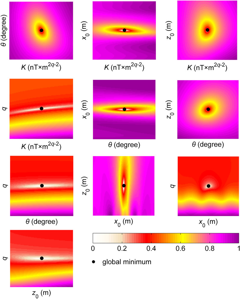
Synthetic magnetic anomaly was generated along a 400 m long profile with 10 m data intervals. We considered a range of values that are half and twice (50% perturbations) the true model parameter values to produce a wide search space for the modal analyses. Figure 3 shows the distributions of the cost function. The middle points of these surface topography maps locate the true values of the source parameter pairs (the global minimum). The distribution maps of θ − K, z0 − K and z0 − θ pairs clearly revealed that the global minima values are enclosed with almost rounded contours and no local ones are situated, which indicates the uni-modal feature72. In short, the parameter pairs are uncorrelated and can most likely be estimated individually by executing an efficient inversion code. However, some elongated valleys and basins with different flat bottoms representing the lowest error function regions displaying the multi-modal73 characteristics were observed in other maps (θ − x0, θ − q, z0 − q, q − x0, q − K, θ − K, and x0 − z0 in Fig. 3), which make the problem complicated, decrease the resolvability characteristics of the source parameters, and increase the uncertainties in the solutions. This means that parameter pairs are correlated with each other. It is well-known fact that banana-shaped contours in objective function surface topographies around the global minimum make precise estimations almost impossible. In our case, we did not observe this kind of topographic features. Thus, model parameters of the non-linear inverse problem presented here can most likely be resolved. Based on these findings, it is clear that the objective function yields the composite modality74 since the uni-modality and multi-modality exist together regarding all model parameter pairs. Error surface topographies of the objective function used indicate the characteristics of non-linearity, high dimensionality and various shapes in paired model spaces, which means that estimations of the model parameters are challenging. However, these difficulties can be overcome with a powerful inversion algorithm which has sufficient ability to approach the global minimum as close as possible without compromising its robustness in order not to be captured by the local minima.
Figure 3.
Modal analyses of the defined objective function for model parameter pairs.
Parameter tuning process
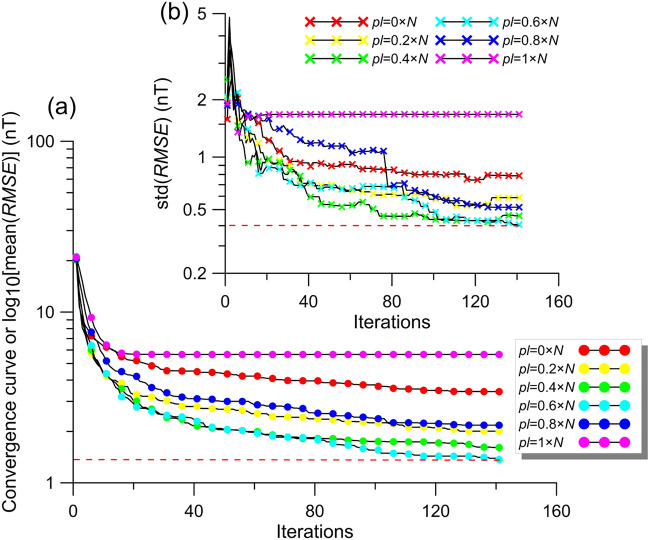
The efficiency of the global optimization algorithm largely depends on fine-tuned control parameters. However, the control parameters proposed by the developers for their own problems or reported ones in previous studies are commonly used for many types of optimization problems. It must be noted that there is no algorithm-based control parameter value that can be successful for all types of inverse problems. These optimal values may vary depending on the nature of inverse problems49,70,75. Hence, a vital step of applying a metaheuristic effectively is to appropriately determine the best user-defined control parameter value/s. As already mentioned, pl plays a key role in defining the exploitation (normal mating process) and exploration stages (sperm cast process) of BMO. To understand the effect of pl values on the solutions a composite noise-free magnetic anomaly due to a multiple-source model was inverted (model parameters are given in Table 2). The search space values used in modal analyses were considered. We used 30 independent runs to suppress the stochastic nature of the metaheuristics so that a more objective evaluation and estimation can be achieved. The optimization processes were performed using 140 iterations and N = 80. As the pl of the BMO varies successively (from 0 × N to 1 × N), the obtained mean RMSE values are displayed in Fig. 4a. Figure 4b demonstrates the variation of the standard deviations (stds) of the calculated RMSE values, indicating the uncertainty of inversion. The variations in the curves (Fig. 4a,b) obtained via various pl values clearly showed that an ill-defined pl value can reduce the performance of the BMO significantly in terms of affecting the solution correctness and the stableness of searching the true parameter values. Additionally, contrary to our expectations, both smaller (e.g., pl = 0 × N) and larger (e.g., pl = 1 × N) pl values caused insufficient performances. By this way, instead of making a random guess based on intuition, the importance of determining the optimum control parameter value/s for the problem of interest was revealed. By performing many trial-and-error tests, we determined that 0.65 is the optimum value for the pl.
Figure 4.
Analyzing the effect of various pl values. (a) Variation behavior of the mean RMSE values obtained via the increment of pl, (b) uncertainties of BMO via the variation of pl.
Inversion studies
We used three synthetic cases with different scenarios to investigate the performance of BMO. The first case discusses a residual magnetic anomaly originated from a multiple-source model given in Table 2. In the second case, we added a regional background effect using a 3rd order polynomial and a local anomaly caused by a near-surface interference (spherical source) to the first case anomaly. In the last case, the second case anomaly was contaminated with a certain degree of random noise (40%). The solutions obtained through the BMO algorithm were compared with those of the sPSO algorithm that uses the suggested9,51 control parameters. Besides, we investigated the performance of the SMA operator in reducing the effect of the regional background. All experiments were conducted on a Windows 10 operating system with Intel(R) Core (TM) i5-6300HQ CPU (2.30 GHz) and 3.8 GB of RAM.
Case 1
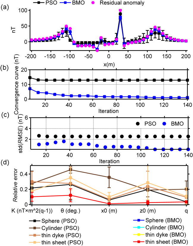
The synthetic magnetic anomaly generated and the causative sources are shown in Fig. 5. We performed 30 independent runs using 80 search agents and 140 iterations for both BMO and sPSO. Table 3 lists the model parameters search spaces and the solutions obtained. Note that the run-time of sPSO and BMO were 74 s and 67 s, respectively. The magnetic anomaly responses calculated through the BMO and sPSO algorithms were compared with the residual magnetic anomaly (Fig. 6a). Figure 6b,c show the behaviors of the mean value and the std of the calculated RMSE values against the iteration number. Figure 6d shows the calculated relative errors of the model parameters recovered via BMO and sPSO approaches. As seen from Fig. 6 and Table 3, the application of BMO algorithm produced stable, accurate, and robust performance. Model parameters with larger error values were obtained with the sPSO application. On the other hand, sPSO showed a faster convergence rate when using large population of search agents. sPSO and BMO converged to global minimum within 20 and 60 iterations, respectively. Although sPSO showed a faster rate of convergence, the resulting RMSE values showed that BMO better achieved an adequate trade-off to balance the exploration and exploitation stages.
Figure 5.
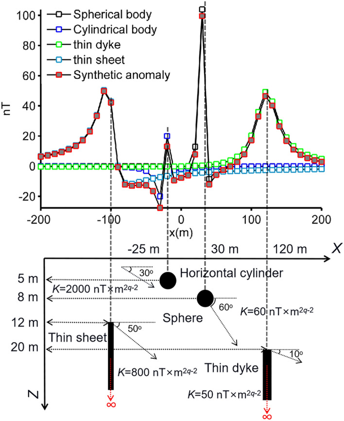
Simulated magnetic anomaly of multiple-source and the causative subsurface model.
Table 3.
Inversion results of the pure residual and contaminated magnetic anomaly caused by multiple-sources using BMO and PSO without and with the implementation of the SMA technique. The order of source structures is as in Table 2.
| Without the implementation of the SMA technique | ||||||
|---|---|---|---|---|---|---|
| Case 1 | ||||||
| Parameter set | True parameters | Search space | PSO results | Relative error | BMO results | Relative error |
| K (nT × m2q−2) | 60/2000/50/800 | 30 ~ 90/1000 ~ 3000/25 ~ 75/400 ~ 1200 | 67.157 ± 18.836/2194.3 ± 630.56/50.053 ± 19.537/766.41 ± 180.01 | 0.21731 ± 0.2215/0.2747 ± 0.0177/0.2998 ± 0.1334/0.1770 ± 0.07898 | 63.058 ± 7.3722/2101.9 ± 245.79/52.549 ± 6.1425/840.77 ± 98.298 | 0.1017 ± 0.0589/0.1017 ± 0.0589/0.1017 ± 0.0589/0.1017 ± 0.0589 |
| θ (degree) | 60/30/10/50 | 30 ~ 90/15 ~ 45/5 ~ 15/25 ~ 75 | 64.14 ± 22.427/25.437 ± 15.857/8.8022 ± 3.6846/38.486 ± 18.097 | 0.2643 ± 0.2050/0.4561 ± 0.0437/0.2769 ± 0.2056/0.3509 ± 0.16049 | 67.292 ± 5.124/33.647 ± 2.5618/11.216 ± 0.85386/56.078 ± 4.27 | 0.1215 ± 0.0854/0.1215 ± 0.0853/0.1215 ± 0.0853/0.1215 ± 0.0853 |
| x0 (m) | 30/− 25/120/− 100 | 15 ~ 45/− 37.5 ~ − 12.5/60 ~ 180/− 150 ~ − 50 | 30.69 ± 2.2587/− 21.693 ± 10.679/117.39 ± 9.9492/− 110.11 ± 5.7627 | 0.0594 ± 0.0340/0.3564 ± 0.1345/0.0699 ± 0.0160/0.1011 ± 0.0576 | 30.008 ± 0.4415/− 24.993 ± 0.3680/120.03 ± 1.7642/− 99.975 ± 1.4717 | 0.0104 ± 0.0073/0.0104 ± 0.0073/0.0104 ± 0.0073/0.0104 ± 0.0073 |
| z0 (m) | 8/5/20/12 | 4 ~ 12/2.5 ~ 7.5/10 ~ 30/6 ~ 18 | 6.4271 ± 0.1128/5.9484 ± 0.4432/21.301 ± 6.8666/10.973 ± 4.8138 | 0.1966 ± 0.0141/0.1896 ± 0.0886/0.2363 ± 0.2011/0.2861 ± 0.2215 | 8.0844 ± 0.2987/5.053 ± 0.1864/20.211 ± 0.7461/12.127 ± 0.4479 | 0.0251 ± 0.0246/0.0251 ± 0.0247/0.0251 ± 0.0246/0.0251 ± 0.0246 |
| q | 2.5/2/1/1 | 1.25 ~ 3.75/1 ~ 3/0.5 ~ 1.5/0.5 ~ 1.5 | 2.4683 ± 0.1031/2.4027 ± 0.2159/1.0848 ± 0.1071/1.1085 ± 0.1109 | 0.035874 ± 0.0035773/0.20137 ± 0.10795/0.096601 ± 0.090866/0.1085 ± 0.11097 | 2.5871 ± 0.0354/2.0697 ± 0.0284/1.0348 ± 0.01420/1.0348 ± 0.0142 | 0.0348 ± 0.0141/0.0348 ± 0.0142/0.0348 ± 0.0142/0.0348 ± 0.0142 |
| RMSE between the uncontaminated magnetic anomaly and the obtained residual responses | 12.8836 ± 2.5283 | 5.3159 ± 0.2323 | ||||
| Case 2 | ||||||
| K (nT × m2q−2) | 54.578 ± 34.758/1194.9 ± 275.63/30.162 ± 7.3005/444.88 ± 63.473 | 0.4096 ± 0.1278/0.4025 ± 0.1378/0.3967 ± 0.1460/0.4439 ± 0.07934 | 66.914 ± 4.0545/1693.8 ± 143.63/55.618 ± 11.24/675.77 ± 56.635 | 0.1152 ± 0.0675/0.1530 ± 0.0718/0.1589 ± 0.1589/0.1552 ± 0.0707 | ||
| θ (degree) | 30 ± 0/30 ± 21.213/14.145 ± 1.2094/41.359 ± 23.135 | 0.5 ± 0/0.5 ± 0/0.4144 ± 0.1209/0.3271 ± 0.2444 | 67.36 ± 13.165/24.475 ± 9.178/11.321 ± 0.58428/48.068 ± 7.3699 | 0.1551 ± 0.1734/0.2163 ± 0.2604/0.1320 ± 0.0584/0.1042 ± 0.0546 | ||
| x0 (m) | 30.529 ± 0.9287/− 28.526 ± 0.5461/155.81 ± 12.113/− 75.298 ± 35.776 | 0.02189 ± 0.0249/0.1410 ± 0.0218/0.298 ± 0.1009/0.2529 ± 0.3493 | 31.016 ± 2.3547/− 21.053 ± 6.1831/142.89 ± 14.63/− 93.811 ± 3.8708 | 0.0555 ± 0.0479/0.1748 ± 0.2232/0.1907 ± 0.1219/0.0618 ± 0.0387 | ||
| z0 (m) | 8.5367 ± 4.8979/7.5 ± 0/16.661 ± 9.4195/6 ± 0 | 0.4329 ± 0.0948/0.5 ± 0/0.3330 ± 0.2361/0.5 ± 0 | 9.1818 ± 1.5044/5.103 ± 0.5569/18.28 ± 0.88362/10.437 ± 5.0416 | 0.1477 ± 0.1880/0.0787 ± 0.0291/0.0860 ± 0.0441/0.2970 ± 0.1841 | ||
| q | 2.9844 ± 0.7070/2.8102 ± 0.2684/0.7169 ± 0.1668/1.2422 ± 0.1495 | 0.2 ± 0.2740/0.4050 ± 0.1342/0.2831 ± 0.1668/0.2421 ± 0.1495 | 2.7649 ± 0.1359/2.2638 ± 0.1980/0.9693 ± 0.05981/1.1929 ± 0.087333 | 0.1059 ± 0.05436/0.1318 ± 0.0990/0.0422 ± 0.0434/0.1929 ± 0.0873 | ||
| RMSE between the contaminated magnetic anomaly and the obtained responses | 40.9405 ± 0.0534 | 45.4893 ± 3.2635 | ||||
| RMSE between the uncontaminated magnetic anomaly and the obtained residual responses | 37.4692 ± 14.9365 | 21.7046 ± 6.7316 | ||||
| With the implementation of the SMA technique (the calculated mean results using different s values are given) | ||||||
| Case 2 | ||||||
| K (nT × m2q−2) | 60/2000/50/800 | 30 ~ 90/1000 ~ 3000/25 ~ 75/400 ~ 1200 | 58.534 ± 11.944/1816.7 ± 328.01/52.685 ± 8.6997/797.78 ± 105.75 | 0.2365 ± 0.0746/0.2241 ± 0.0808/0.2053 ± 0.1000/0.1786 ± 0.0878 | 60.623 ± 1.7993/2037.3 ± 74.326/48.386 ± 1.9889/777.27 ± 43.932 | 0.0607 ± 0.0212/0.0638 ± 0.0373/0.0608 ± 0.0258/0.0684 ± 0.0276 |
| θ (degree) | 60/30/10/50 | 30 ~ 90/15 ~ 45/5 ~ 15/25 ~ 75 | 63.913 ± 7.9871/31.838 ± 5.4413/10.933 ± 2.0296/49.247 ± 9.219 | 0.2168 ± 0.0727/0.1842 ± 0.03944/0.1938 ± 0.0939/0.1845 ± 0.0957 | 58.764 ± 4.401/28.553 ± 2.3802/9.7616 ± 0.79822/48.119 ± 3.4934 | 0.0532 ± 0.0575/0.0772 ± 0.0568/0.0681 ± 0.0513/0.0775 ± 0.0458 |
| x0 (m) | 30/− 25/120/− 100 | 15 ~ 45/− 37.5 ~ − 12.5/60 ~ 180/− 150 ~ − 50 | 30.041 ± 0.60487/− 24.432 ± 1.2435/115.59 ± 17.989/− 98.297 ± 8.158 | 0.0199 ± 0.0119/0.0483 ± 0.0645/0.1867 ± 0.0797/0.0672 ± 0.0707 | 29.965 ± 0.2545/− 24.801 ± 0.5644/120.37 ± 3.3909/− 99.84 ± 2.0854 | 0.0193 ± 0.0080/0.0205 ± 0.0118/0.0273 ± 0.0166/0.02417 ± 0.0109 |
| z0 (m) | 8/5/20/12 | 4 ~ 12/2.5 ~ 7.5/10 ~ 30/6 ~ 18 | 7.1768 ± 1.0318/4.7307 ± 0.7216/17.265 ± 2.3129/11.51 ± 1.6127 | 0.2029 ± 0.0524/0.1721 ± 0.097/0.2195 ± 0.0881/0.2103 ± 0.0602 | 7.9239 ± 0.4027/5.0283 ± 0.3071/19.856 ± 0.8801/12.324 ± 0.578 | 0.0590 ± 0.0234/0.0791 ± 0.0329/0.0561 ± 0.0244/0.056511 ± 0.02568 |
| q | 2.5/2/1/1 | 1.25 ~ 3.75/1 ~ 3/0.5 ~ 1.5/0.5 ~ 1.5 | 2.4956 ± 0.0287/2.1173 ± 0.1719/1.0472 ± 0.0861/1.0499 ± 0.10461 | 0.0166 ± 0.0076/0.0849 ± 0.0607/0.1906 ± 0.0991/0.1164 ± 0.0629 | 2.5159 ± 0.0232/2.0363 ± 0.0286/1.0108 ± 0.0194/1.011 ± 0.0212 | 0.0089 ± 0.0076/0.0210 ± 0.0135/0.0283 ± 0.0227/0.0286 ± 0.0273 |
| RMSE between the calculated SMA magnetic anomalies and the inverted ones | 18.3725 ± 0.2184 | 15.8042 ± 0.5604 | ||||
| RMSE between the uncontaminated magnetic anomaly and the obtained residual responses | 23.9215 ± 10.1662 | 5.5187 ± 0.8829 | ||||
| Case 3 | ||||||
| K (nT × m2q−2) | 64.628 ± 13.693/2251 ± 214.83/50.535 ± 5.3922/811.02 ± 205.46 | 0.2133 ± 0.0741 /0.2104 ± 0.0787/0.2299 ± 0.0646/0.2368 ± 0.0511 | 60.135 ± 3.6594/2005.6 ± 168.49/50.706 ± 2.5656/788.2 ± 63.652 | 0.0823 ± 0.0498/0.0760 ± 0.0312/0.0741 ± 0.0199/0.0748 ± 0.0271 | ||
| θ (degree) | 66.58 ± 8.3505/31.9 ± 6.9616/10.052 ± 1.3155/54.51 ± 8.1819 | 0.2119 ± 0.0837/0.2022 ± 0.0979/0.1883 ± 0.0935/0.2179 ± 0.0574 | 59.292 ± 3.9508/29.679 ± 1.3942/9.884 ± 0.26552/49.094 ± 3.2371 | 0.0618 ± 0.0380/0.0493 ± 0.0324/0.0408 ± 0.0203/0.06890 ± 0.0390 | ||
| x0 (m) | 29.58 ± 0.68447/− 25.127 ± 1.1433/127.74 ± 21.46/− 91.905 ± 10.83 | 0.0277 ± 0.0219/0.0491 ± 0.0385/0.1754 ± 0.119/0.0810 ± 0.1082 | 29.978 ± 0.5206/− 24.901 ± 0.7025/120.3 ± 3.157/− 99.408 ± 0.4812 | 0.0217 ± 0.0082/0.0311 ± 0.0167/0.0302 ± 0.0183/0.01188 ± 0.01176 | ||
| z0 (m) | 8.683 ± 0.6031/5.3544 ± 0.7323/19.928 ± 2.6287/11.909 ± 1.2843 | 0.1785 ± 0.0674/0.1855 ± 0.0517/0.1735 ± 0.0820/0.1779 ± 0.05247 | 8.2001 ± 0.3039/5.0115 ± 0.2916/19.23 ± 1.3641/12.113 ± 0.32479 | 0.0636 ± 0.0105/0.0704 ± 0.0345/0.0660 ± 0.0548/0.0566 ± 0.0383 | ||
| q | 2.5001 ± 0.0561/2.0916 ± 0.1450/1.0016 ± 0.1319/1.0419 ± 0.1449 | 0.0186 ± 0.0133/0.074481 ± 0.0449/0.15597 ± 0.0725/0.1537 ± 0.0612 | 2.5211 ± 0.0486/2.0138 ± 0.0402/0.9876 ± 0.0299/0.9944 ± 0.0207 | 0.0160 ± 0.0124/0.0188 ± 0.0097/0.0339 ± 0.0221/0.02533 ± 0.0171 | ||
| RMSE between the calculated SMA magnetic anomalies and the inverted ones | 23.1848 ± 0.8570 | 21.2171 ± 0.4926 | ||||
| RMSE between the uncontaminated magnetic anomaly and the obtained residual responses | 28.1128 ± 6.7413 | 7.0089 ± 2.5616 | ||||
Significant values are in bold.
Figure 6.
Inversion results of case 1. (a) fittings between the simulated residual magnetic anomaly and the responses obtained via BMO and sPSO, (b) the variation behavior of the mean RMSE values against iterations after 30 runs, (c) the variation behavior of the std of RMSE values against iterations after 30 runs, (d) calculated relative errors of model parameter solutions using BMO and sPSO for four causative sources. Error bars are given in (a) and (d).
Case 2
In this experiment we added regional and local effects to the synthetically generated magnetic anomaly using the following expressions:
| 16 |
| 17 |
| 18 |
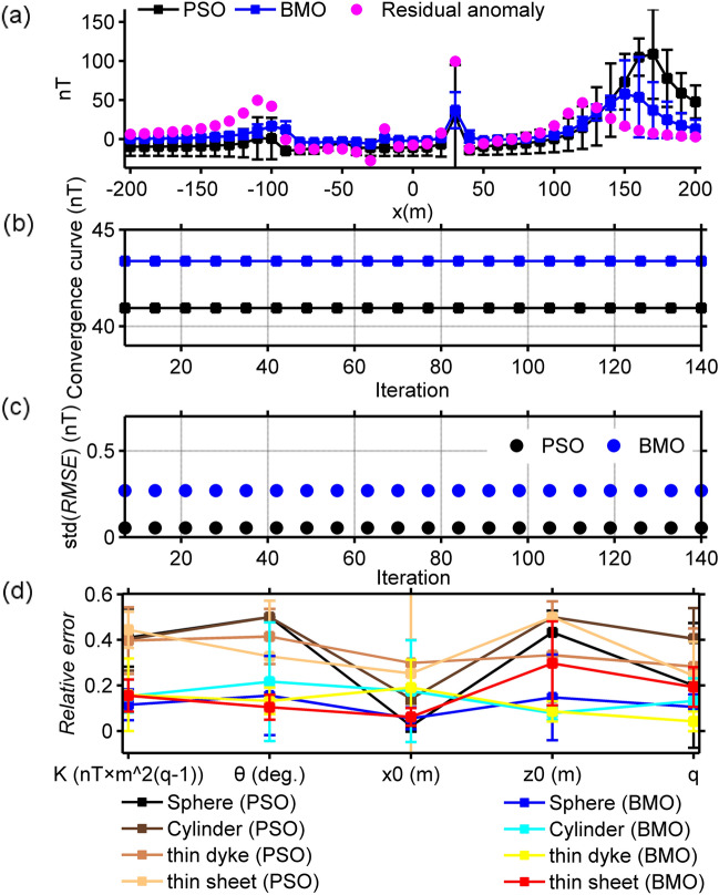
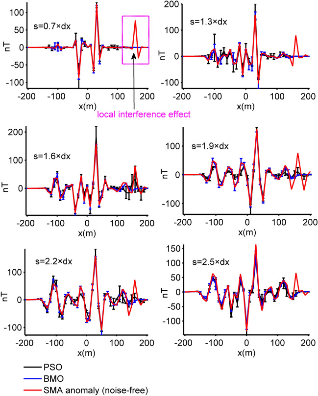
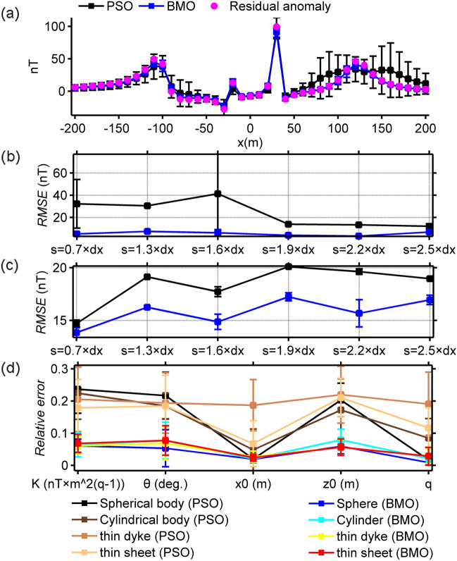
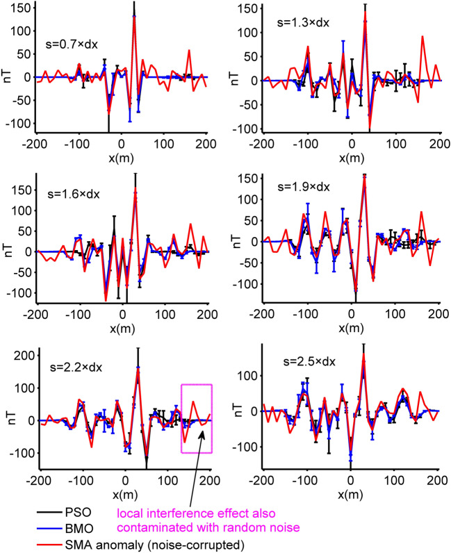
where denotes the composite anomaly, Tre(xi) is the regional background effect and Tlocal(xi) represents the local perturbation originated from a near-surface spherical interference. Figure 7 illustrates the subsurface magnetized sources and the resulting magnetic responses. BMO and sPSO were applied using 30 independent runs with 80 search agents and 140 iterations. The control parameters of both optimizers were kept unchanged, and applications were performed without using the SMA technique. Search space bounds consistent with the first case were used. After each iteration, the mean, std of RMSE values, and the relative errors of estimated parameters were recorded to observe the performances (Fig. 8). Table 3 stores the quantitative results of estimations. The run-time of sPSO and BMO algorithms were 69 s and 66 s, respectively. It is clear that the mean RMSE value increased significantly with the final iteration. Moreover, the error values between the calculated and the true model parameters of four causative sources increased too. It is clear that both algorithms underperformed due to the presence of external effects incorporated. Subsequently, we experienced the effectiveness of the SMA technique in reducing the regional effects. Figure 9 illustrates the calculated SMA magnetic anomalies (red lines) for some s values (0.7, 1.3, 1.6, 1.9, 2.2, and 2.5 × dx, dx equals the data spacing interval). Blue and black lines represent the calculated responses obtained through BMO and sPSO, respectively and are generally in well agreement with the red lines except for the anomalies generated from the interfering shallow spheric source. In this scenario, the running times of the sPSO and BMO algorithms are equal to the product of the times given previously and the s-values used, namely 69 s and 66 s. Hence, we will solely present the computational time considering the circumstance of delineating the residual anomaly. Outputs of this synthetic experiment and the detailed inversion results are shown in Fig. 10 and Table 3, respectively. It is clear that the SMA technique proved useful in eliminating the regional effect from the composite magnetic anomaly and therefore both algorithms yielded relatively agreeable results. However, examining the results in detail, it is seen that the mathematical nature of simulating the special mating behaviors of barnacles yielded lower fitness errors, more accurate model parameter values, and higher inversion stability than sPSO.
Figure 7.
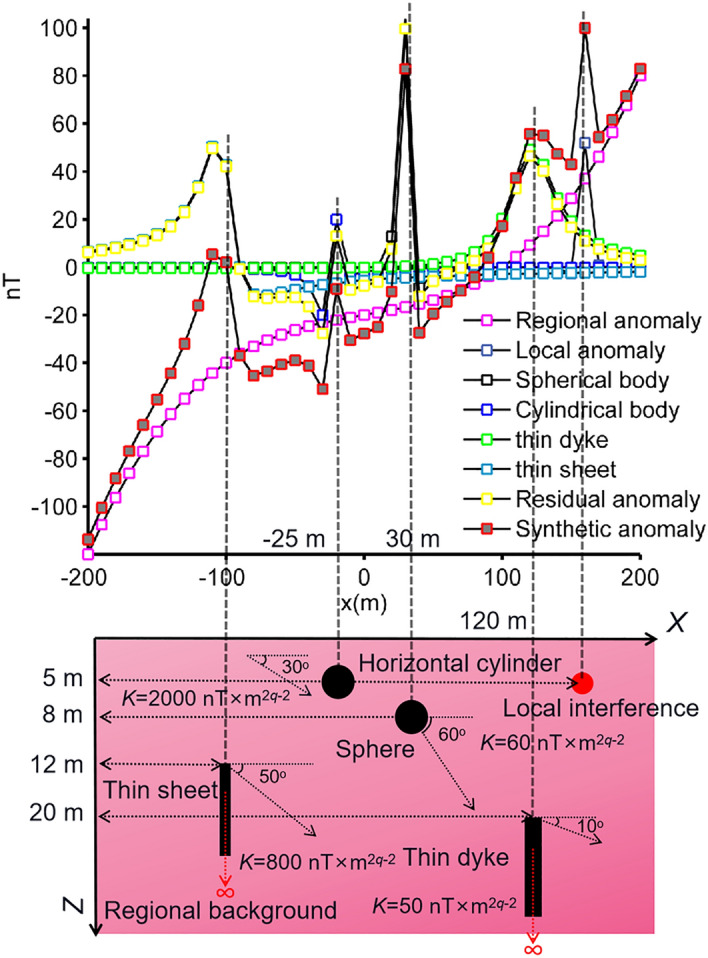
Synthetic residual magnetic anomaly of the multiple-source model (case 2) superposed on a regional background and local interference, and the causative subsurface model.
Figure 8.
Inversion results of case 2 without the implementation of the SMA technique. (a) fittings between the pure residual magnetic anomaly and the responses obtained via BMO and sPSO, (b) the variation behavior of the mean RMSE values against iterations after 30 runs, (c) the variation behavior of the std of RMSE values against iterations after 30 runs, (d) calculated relative errors of model parameter solutions using BMO and sPSO for four causative sources. Error bars are given in (a) and (d).
Figure 9.
The calculated SMA magnetic anomalies of case 2 and estimated SMA magnetic responses using BMO and sPSO for different s values (0.7, 1.3, 1.6, 1.9, 2.2, and 2.5 × dx, dx = 10 m).
Figure 10.
Inversion results of case 2 with the implementation of the SMA technique. (a) fittings between the pure residual magnetic anomaly and the responses obtained via BMO and sPSO, (b) variation behavior of the calculated RMSE values between the uncontaminated magnetic anomaly of case 1 and the residual responses obtained via BMO and sPSO for different s values, (c) variation behaviors of the computed RMSE values between the calculated SMA magnetic anomalies of case 2 and the estimated SMA magnetic responses of BMO and sPSO for different s values, (d) relative errors of the calculated average estimation of the obtained model parameters using BMO and sPSO for four causative sources from the SMA magnetic anomalies for several s values. Error bars are given in (a)–(d).
Case 3
In order to make the work of both algorithms more difficult, a noise content of 40% was added to the magnetic anomaly of case 2 by using the definition below:
| 19 |
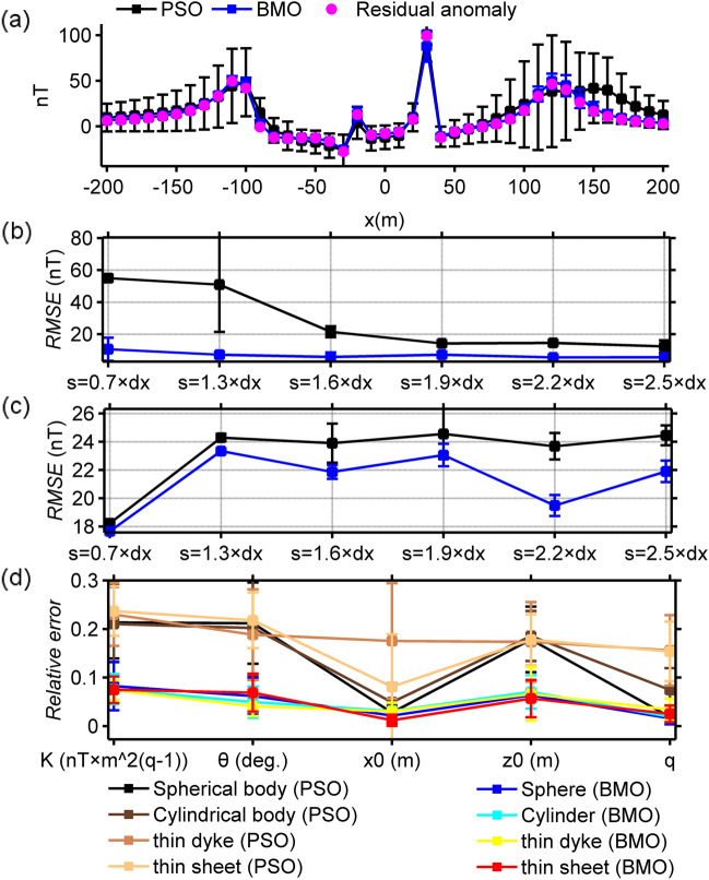
where mean() is the average value of the input, rand1() and rand2() return an array containing pseudorandom values between [0, 1] of a given size. Using the same computation procedures, we inverted the synthetic magnetic anomaly through both algorithms. The SMA noisy anomaly and estimated SMA magnetic responses obtained by means of BMO and sPSO (blue and black solid lines) for different s values are demonstrated in Fig. 11. Figure 12 and Table 3 show the outputs of the optimization via both algorithm and detailed inversion results, respectively. Applications showed that the added 40% random noise only produced minor perturbations to the SMA residual anomalies (red lines in Fig. 11). Both algorithms produced satisfactory solutions, but the details revealed the superiority of BMO in terms of lower error values, more accurate model parameter values, and more stable optimization.
Figure 11.
The SMA results of 40% random noise-corrupted magnetic anomalies of case 2 and estimated SMA magnetic responses via BMO and sPSO for different s values (0.7, 1.3, 1.6, 1.9, 2.2, and 2.5 × dx, dx = 10 m).
Figure 12.
Inversion results of case 3 with the implementation of the SMA technique. (a) fittings between the residual magnetic anomaly and the responses obtained via BMO and sPSO, (b) variation behaviors of the calculated RMSE values between the uncontaminated magnetic anomaly of case 1 and the residual responses obtained via BMO and sPSO for different s values, (c) variation behaviors of the computed RMSE values between the calculated SMA magnetic anomalies of case 3 and the estimated SMA magnetic responses of BMO and sPSO for different s values, (d) relative errors of the calculated average estimation of the obtained model parameters using BMO and sPSO for four causative sources from the SMA magnetic anomalies for different s values. Error bars are also given in (a)–(d).
Post-inversion uncertainty appraisal analysis of synthetic case
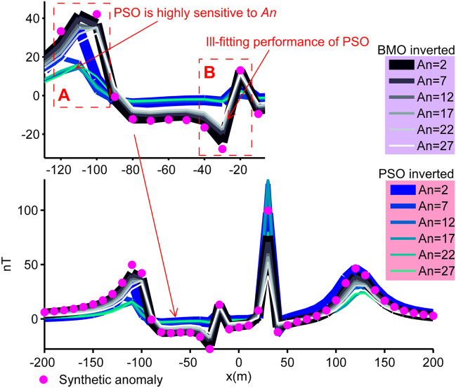
As mentioned previously in the modal analysis section, the optimization problem presented here is mostly unstable and error-prone because of the extreme complexity of escaping massive local minima while effectively exploiting the unique global minimum. Therefore, post-inversion uncertainty assessment analyses are crucial for understanding the credibility of the model parameters recovered. To practice the uncertainty appraisal studies, we used the solutions obtained in the first case experiment. Best model parameters obtained in each independent runs were listed and then sorted in ascending order of their misfit values. We assumed An as a variable in order to determine the number of sorted parameters. That we used to compute the final results by calculating the mean responses. We considered An as a variable to determine the number of parameters sorted. We then calculated the mean of each sorted parameter values. Lastly, the mean magnetic anomaly response was obtained with the mean model parameter set. Figure 13 exhibits that BMO showed low sensitivity to the increment of An, however, the performance of sPSO was significantly affected with the use of larger An values (pointed part A). Consistently, this phenomenon is correlated with the larger std values in the inversion results of sPSO. On the other hand, the superiority of the anomaly-fitting ability of BMO regardless the value of An is clearly observed in pointed part B (Fig. 13). These findings clearly revealed that BMO is more capable than sPSO in obtaining more robust solutions for this inverse problem presented.
Figure 13.
Post-inversion uncertainty appraisal analyses. Calculated mean responses of both algorithms varying with An (case 1).
Real data applications
The performance of BMO in the inversion of real magnetic anomalies was tested using three field cases from India and Brazil. These magnetic anomalies were considered as residual responses and were studied by some researchers using several data processing techniques. Based on this information, we initially treated these data sets as residual magnetic anomalies and applied the BMO algorithm using pl = 0.65 × N. We applied sPSO using the same algorithm-based control parameters to obtain outputs for the comparison tests. In the experiments, both algorithms were run independently 30 times using 80 search agents and 140 iterations. We then applied BMO procedure to SMA anomalies to understand if these anomalies are contaminated by regional background effect and/or local interference. Finally, the model parameter solutions obtained were interpreted in an integrated manner with the known geological data and/or previous geophysical estimates given in Table 4.
Table 4.
Reported results of the field cases.
| Chromite Ore, Tangarparha, Odisha, India | |||||
|---|---|---|---|---|---|
| Parameter set | K (nT × m2q−2) | x0 (m) | z0 (m) | θ (degree) | q |
| Biswas (2018) | − 118.93 ± 0.69/370.01 ± 05/− 143.22 ± 1.04 | 45.77 ± 0.57/825.20 ± 0.20/1062.16 ± 1.22 | 150.36 ± 0.31/344.30 ± 0.70/261.43 ± 2.17 | 163.75 ± 0.34/0.00 ± 0.5/4.64 ± 0.39 | 2.5/2.5/2.5 |
| Uranium Ore, Beldih Mine, Purulia, West Bengal, India | |||||
| Biswas (2018) | 779.86 ± 1.17/3183.15 ± 8.71/1760.56 ± 10.80 | 110.74 ± 0.03/166.14 ± 0.21/255.71 ± 1.38 | 8.39 ± 0.02/34.26 ± 0.10/25.72 ± 0.67 | 57.95 ± 0.15/54.89 ± 0.37/− 2.45 ± 4.83 | 1/1/1 |
| Parnaiba anomaly, Brazil | |||||
| Biswas (2018) | − 1541.27 ± 16.05 | 0.57 ± 0.02 | 3.47 ± 0.03 | 59.24 ± 0.30 | 2 |
| Tlas and Asfahani (2015) | − 645.6 | 0 | 3.4 | 41.3 | 2 |
| Abdelrahman and Essa (2015) | – | – | 2.35 | – | 1.02 |
| Asfahani and Tlas (2007) | − 59.8 | – | 2.3 | 47.1 | – |
| Asfahani and Tlas (2004) | − 59.81 | – | 2.26 | 47.11 | – |
| Abdelrahman and Sharafeldin (1996) | − 58.6 | – | 3.5 | 33.3 | – |
| Silva (1989) | – | – | 3.5 | – | – |
Chromite Ore Anomaly, India
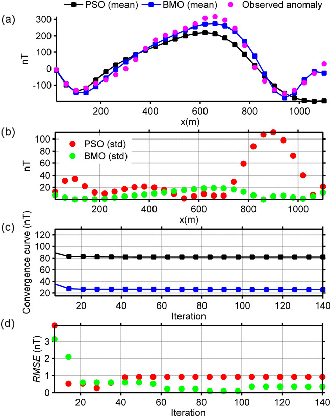
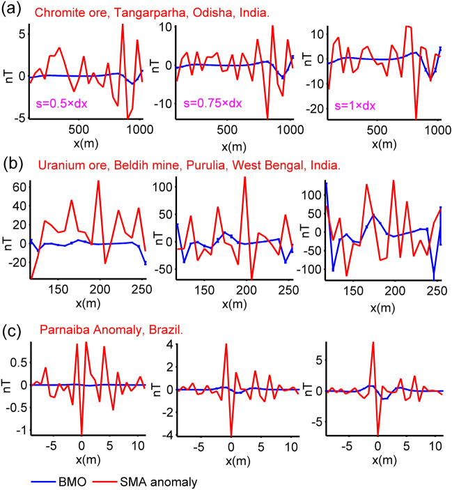
The studied chromite ores are located in Tangarparha, Odisha, India. According to prior information, the ore bodies in this area are known to have a pod-type structure that is more reminiscent of a sphere-shaped source12. The magnetic anomaly response12,76 of these magnetized sources is presented in Fig. 14a with pink circles. The data sampling interval is 40 m for this anomaly. This anomaly was studied previously by using Very Fast Simulated Annealing (VFSA) technique with various source assumptions such as single spherical-shaped body, cylinder, dyke, and sheet12. This magnetic anomaly was interpreted to originate from three spherical source bodies12. Model parameter solutions revealed in that study are given in Table 4. First, we considered this finding and applied the BMO and sPSO algorithms to estimate the model parameters. Search space bounds for model parameters are given in Table 5. Figure 14a displays the comparison between the observed data and the reconstructed mean responses. Figure 14b shows the calculated std values of obtained responses at each station. The mean value and std of RMSE against the iterations for 30 independent runs are shown in Fig. 14c,d. Table 5 lists the obtained model solutions (K, θ, x0, z0, q) and RMSEs. The run-time of sPSO and BMO were 65 s and 59 s, respectively. The inversion results indicated that the assumed three spherical bodies approximate the sources effectively. Despite the faster convergence rate of sPSO, BMO outperformed in terms of response-fitting and stability. In the next step, we applied BMO to the SMA anomaly (s = 0.5, 0.75, and 1 × dx, dx = 40 m). Figure 17a displays the SMA results (red lines) for various s values and obtained responses (blue lines). Notably, model parameters obtained using the SMA technique (Table 5) are in well agreement with the results accomplished from considering the acquired data as a pure residual response. This finding indicates that the observed magnetic response does not contain undesired structural information such as regional background and near-surface source effects, but may contain random noise. The solutions obtained here are relatively in well agreement with the ones achieved via VFSA (Table 5).
Figure 14.
Inversion results of the chromite ore anomaly, India. (a) fittings between the observed magnetic anomaly and the mean responses obtained via BMO and sPSO, (b) calculated std values of obtained responses at each station, (c) variation behavior of the mean RMSE values against iterations of BMO and sPSO after 30 independent runs, (d) variation behavior of the std of RMSE values against iterations of BMO and sPSO after 30 runs.
Table 5.
Inversion results of the field magnetic anomalies using BMO and PSO without and with the implementation of the SMA technique.
| Chromite Ore, Tangarparha, Odisha, India | |||
|---|---|---|---|
| Without the implementation of the SMA technique | |||
| Parameter set | Search spaces | PSO results | BMO results |
| K (nT × m2q−2) | − 124.88 ~ − 41.626/230.91 ~ 692.74/− 150.15 ~ − 50.05 | − 89.911 ± 0/532.39 ± 33.388/− 108.11 ± 0 | − 83.456 ± 0.5482/460.69 ± 3.0421/− 100.35 ± 0.6592 |
| θ (degree) | 80.154 ~ 240.46/0 ~ 0/1.2652 ~ 3.7957 | 156.14 ± 0.8431/0 ± 0/2.7927 ± 0.7742 | 158.86 ± 1.115/0 ± 0/2.5077 ± 0.017604 |
| x0 (m) | 24.259 ~ 72.777/477.53 ~ 1432.6/494.74 ~ 1484.2 | 49.481 ± 0.9878/841.03 ± 56.92/1081.3 ± 317.91 | 48.976 ± 0.1202/964.07 ± 2.3662/998.81 ± 2.4534 |
| z0 (m) | 112.4 ~ 337.21/254.18 ~ 762.53/103.96 ~ 311.89 | 181.3 ± 27.483/457.75 ± 129.73/272.66 ± 2.5461 | 224.57 ± 1.906/507.82 ± 4.3115/207.7 ± 1.7627 |
| q | 1.213 ~ 3.6391/1.2523 ~ 3.757/1.1962 ~ 3.588 | 2.4537 ± 0.0038/2.5574 ± 0.0048/2.8354 ± 0.0289 | 2.43 ± 0.0042/2.5087 ± 0.0043/2.3961 ± 0.0042 |
| RMSE between the observed magnetic anomaly and the obtained residual responses | 82.0409 ± 0.9173 | 29.6877 ± 0.6917 | |
| With the implementation of the SMA technique (the mean output of various dx) | |||
| K (nT × m2q−2) | − 83.42 ± 0.2328/508.09 ± 1.3828/− 100.18 ± 0.2201 | ||
| θ (degree) | 160 ± 0.4774/0 ± 0/1.2748 ± 0.0046261 | ||
| x0 (m) | 38.92 ± 0.12763/968.77 ± 3.514/993.73 ± 3.3938 | ||
| z0 (m) | 320.11 ± 1.6701/540.34 ± 2.2061/247.09 ± 1.1117 | ||
| q | 2.4318 ± 0.0187/2.5016 ± 0.0195/2.3785 ± 0.0197 | ||
| RMSE between the calculated SMA magnetic anomalies and the inverted one | 4.2777 ± 0.0010 | ||
| Uranium Ore, Beldih Mine, Purulia, West Bengal, India | |||
| Without the implementation of the SMA technique | |||
| K (nT × m2q−2) | 500.71 ~ 1502.1/1887 ~ 5660.9/761.75 ~ 2285.2 | 1072.1 ± 174.09/3614.6 ± 1287.4/1934.5 ± 293.66 | 1018.1 ± 1.5033/3836.9 ± 5.7627/1548.9 ± 2.2656 |
| θ (degree) | 18.261 ~ 54.783/30.131 ~ 90.393/− 1.8007 ~ − 0.600 | 40.125 ± 3.3586/61.178 ± 24.724/− 1.1525 ± 0 | 36.585 ± 0.0702/60.365 ± 0.1153/− 1.1984 ± 0.0023 |
| x0 (m) | 55.468 ~ 166.4/83.652 ~ 250.96/129.37 ~ 388.11 | 98.389 ± 26.253/165.61 ± 12.337/221.96 ± 53.706 | 110.61 ± 0.2385/166.81 ± 0.3524/257.97 ± 0.5643 |
| z0 (m) | 6.97 ~ 20.91/16.086 ~ 48.258/5.8273 ~ 17.482 | 15.849 ± 5.9752/44.571 ± 2.4841/7.459 ± 0 | 13.957 ± 0.2744/32.21 ± 0.6317/11.669 ± 0.22926 |
| q | 0.4635 ~ 1.3908/0.5155 ~ 1.5466/0.57816 ~ 1.7345 | 1.0296 ± 0.15337/1.0319 ± 0.0465/1.3087 ± 0.0335 | 0.9303 ± 0.0010/1.0346 ± 0.0012/1.1602 ± 0.00125 |
| RMSE between the observed magnetic anomaly and the obtained residual responses | 262.6028 ± 63.7970 | 119.7986 ± 2.7188 | |
| With the implementation of SMA technique (the mean output of various dx) | |||
| K (nT × m2q−2) | 1135.2 ± 5.4598/4474.1 ± 32.224/1402.1 ± 7.4276 | ||
| θ (degree) | 32.261 ± 0.1291/55.003 ± 0.1336/− 0.8413 ± 0.0025 | ||
| x0 (m) | 111.21 ± 0.1963/168.96 ± 0.5606/259.28 ± 1.4854 | ||
| z0 (m) | 13.646 ± 0.0696/33.115 ± 0.1668/11.665 ± 0.0575 | ||
| q | 0.9786 ± 0.0012/1.0582 ± 0.0046/1.1005 ± 0.0036 | ||
| RMSE between the calculated SMA magnetic anomalies and the inverted one | 41.0148 ± 0.1821 | ||
| Mesozoic dyke anomaly, Brazil | |||
| Without the implementation of the SMA technique | |||
| K (nT × m2q−2) | − 2003.3 ~ − 1078.7 | − 1195.3461 ± 160.9861 | − 1518.7165 ± 4.3658 |
| θ (degree) | 41.468 ~ 77.012 | 41.7885 ± 0.1377 | 36.0851 ± 0.1544 |
| x0 (m) | 0.399 ~ 0.741 | 0.6333 ± 0.0131 | 0.6598 ± 0.0590 |
| z0 (m) | 2.429 ~ 4.511 | 4.5077 ± 0.0025 | 5.7835 ± 0.0166 |
| q | 1.4 ~ 2.6 | 2.0248 ± 0.0348 | 1.9700 ± 0.0030 |
| RMSE between the observed magnetic anomaly and the obtained residual responses | 7.8110 ± 0.0174 | 4.7079 ± 0.0442 | |
| With the implementation of the SMA technique (the mean output of various dx) | |||
| K (nT × m2q−2) | − 1531.4377 ± 84.6412 | ||
| θ (degree) | 32.3969 ± 0.8404 | ||
| x0 (m) | 0.84221 ± 0.0061 | ||
| z0 (m) | 5.2524 ± 0.0488 | ||
| q | 2.1250 ± 0.0342 | ||
| RMSE between the calculated SMA magnetic anomalies and the inverted one | 1.0191 ± 0.0001 | ||
Significant values are in bold.
Figure 17.
Inversion results of three field cases obtained via BMO with the implementation of the SMA technique, (a) the calculated SMA magnetic anomalies of the chromite ore anomaly, India and estimated response of BMO for different s values (0.5, 0.75, and 1 × dx, dx = 40 m), (b) the calculated SMA magnetic anomalies of the uranium ore anomaly, India and estimated response of BMO for different s values (0.5, 0.75, and 1 × dx, dx = 8 m), (c) the calculated SMA magnetic anomalies of the Mesozoic dyke anomaly, Brazil and estimated response of BMO for different s values (0.5, 0.75, and 1 × dx, dx = 0.8 m).
Uranium Ore Anomaly, India
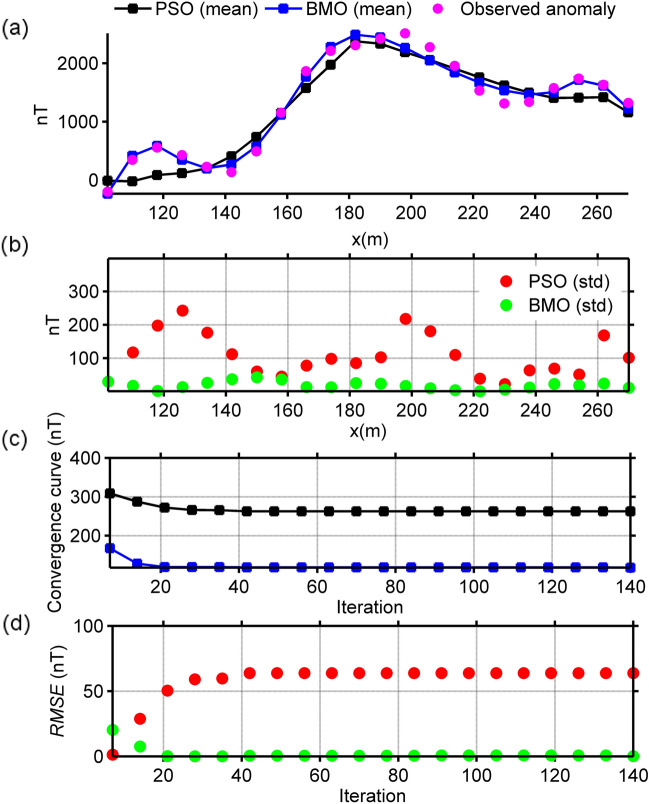
The magnetic anomaly sampled at 8 m interval in the Beldih mine (Purulia, West Bengal, India) is caused from uranium ore bodies77. Some previous studies revealed that the uranium ore bodies in this part can be represented with vertical thick-sheet-like structures as deciphered from spontaneous-potential data interpretation78–80. This interpretation was validated by drilling results81, which disclosed that mineralization begins from the near-surface and extends to the depths of 10–20 m and which are approximately vertical and dipping northerly to southerly12. Additionally, gravity and resistivity responses were also used to understand subsurface nature of the source structures77,82,83. Lastly, this magnetic anomaly was interpreted12 using the VFSA technique considering dyke-like source as equal to thick-sheet-type source (Table 4). Similarly, we considered it as a residual response due to multiple dyke-like structures and implemented BMO and sPSO algorithms for reinterpretation. The model parameter ranges of assumed dykes and the results obtained are listed in Table 5. The run-time of sPSO and BMO were 54 s and 48 s, respectively. The comparison of the calculated magnetic responses with the observed one is illustrated in Fig. 15a. Figure 15b depicts the calculated std values of the obtained responses at each measurement point. Figure 15c,d demonstrates the mean value and std values of RMSE against the iteration number. It can be clearly seen that the anomaly of the assumed multiple dyke-like structures matches well with the observed one and BMO provides appealing results in terms of escaping local minima, fitting errors and stability of the inversion compared to those obtained via sPSO. Figure 17b illustrates the SMA anomalies (red lines) for s = 0.5, 0.75, and 1 × dx (dx = 8 m) and reconstructed responses via BMO (blue lines). An obvious difference between the calculated and the reconstructed responses is seen. Nevertheless, recovered model parameters given in Table 5 are correspond to the solutions obtained without the implementation of the SMA scheme. Thus, it was verified that the observed anomaly is most likely corrupted by the local interference effect and/or random noise.
Figure 15.
Inversion results of the uranium ore anomaly, India. (a) fittings between the observed magnetic anomaly and the mean responses obtained via BMO and sPSO, (b) calculated std values of obtained responses at each station, (c) variation behavior of the mean RMSE values against iterations of BMO and sPSO after 30 independent runs, (d) variation behavior of the std of RMSE values against iterations of BMO and sPSO after 30 runs.
Mesozoic dyke Anomaly, Brazil
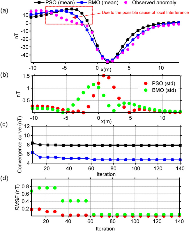
Figure 16a shows a magnetic anomaly observed on a Mesozoic dyke that intruded into Paleozoic sedimentary rocks in the Parnaiba basin, Brazil84. The data sampling interval is 0.8 m. This anomaly was previously interpreted using different approaches12,26,84,85 assuming a horizontal cylinder along with thin-sheet structure. Solutions reported in those studies are given in Table 4. Here, this magnetic anomaly was studied using BMO and sPSO algorithms, considering it the response of a cylindrical body. Model parameter search bounds used are listed in Table 5. The run-time of sPSO and BMO were 20 s and 18 s, respectively. Estimated mean responses through BMO and sPSO are displayed in Fig. 16a, which closely match with the measured one (pink circles). However, the unsatisfactory performances of sPSO and BMO are observed at the pointed part shown in Fig. 16a. The possible explanation for this case is the presence of the local interference effect. Figure 16b demonstrates the calculated std values of obtained responses at each measurement station. Figure 16c,d display the mean value and std values of RMSE against the iterations. Table 5 gives the estimated model parameters. Findings showed that BMO yields better performance in terms of relatively lower misfit values and higher stability again. Figure 17c shows a comparison between the calculated SMA results for various s values (s = 0.5, 0.75, and 1 × dx, dx = 0.8 m), and regenerated responses using BMO. The estimated source parameters are listed in Table 4 along with misfits. Accordingly, it can be mentioned that BMO produced steady solutions with those delineated from considering the observed data as a pure residual response. Calculated anomalies of the BMO, however, revealed obvious differences most likely due to the existence of local interference effects and/or random noises. Thus, we concluded that the observed magnetic anomaly does not contain remarkable regional component, but may contain some amount of local perturbation and/or random noise.
Figure 16.
Inversion results of the Mesozoic dyke anomaly, Brazil. (a) fittings between the observed magnetic anomaly and the mean responses obtained via BMO and sPSO, (b) calculated std values of obtained responses at each station, (c) variation behavior of the mean RMSE values against iterations of BMO and sPSO after 30 independent runs, (d) variation behavior of the std of RMSE values against iterations of BMO and sPSO after 30 runs.
Post-inversion uncertainty appraisal analyses of real data cases
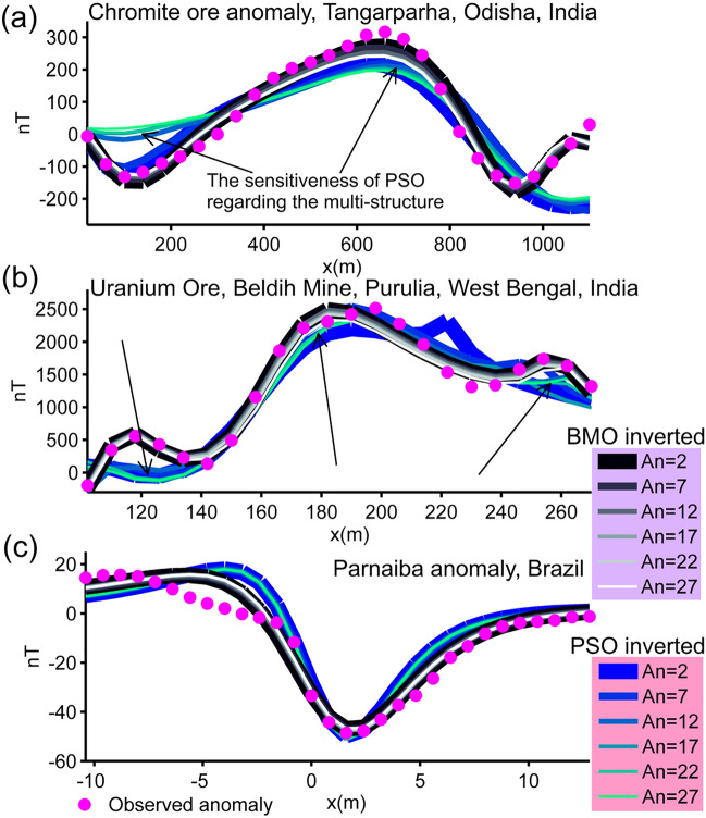
The reliability of the model parameters obtained was investigated, as in the synthetic experiments on the basis of the solutions of 30 independent runs for all real data cases. Figure 18 shows the variation characteristics of computed responses using different An values. It can be easily observed that the performance of the sPSO was affected with a larger An regarding the first two multiple-source model, especially in the pointed parts. This fact correlates with the large std values as discussed before. On the contrary, BMO is generally insensitive to a larger An, which indicates the superiority of the BMO in handling more complicated cases. Notably, as for the single structure model, only minor variations occurred in the responses of BMO and sPSO. However, when comparing the best performances of both approaches using An = 2 it is again apparent that BMO provided better fitting performance in these real data cases, since it offers sufficient opportunities to escape massive local minima while effectively exploiting the global minimum.
Figure 18.
Post-inversion uncertainty appraisal analyses of field data sets using computed mean responses of BMO and sPSO with different An. (a) chromite ore anomaly, India, (b) uranium ore anomaly, India, (c) Mesozoic dyke anomaly, Brazil.
Conclusions
BMO, a novel nature-inspired derivative-free global optimizer, was presented for the inversion of magnetic anomalies. Modal analyses helped us understand the characteristic of the inverse problem. Finely-tuned control parameter increased the effectiveness of the optimizer. Satisfactory solutions were obtained in both synthetic and real data cases. SMA technique successfully suppressed the regional background effects. The effectiveness of BMO was compared with sPSO, the most widely used metaheuristic in geophysical inverse problems. The reliability of the results produced by both algorithms was tested with uncertainty analysis. Applications showed that BMO produced more stable and more robust solutions for the cases used in this study. It was also observed that BMO completed the optimizations in relatively less run-time than sPSO. Besides, the model parameters obtained for the real data cases are in agreement with the available geologic and/or geophysical information. Based on these findings, we concluded that BMO is more efficient than sPSO in balancing global exploration (the ability to explore the search space extensively and escape the capture of massive local minima) and the local exploitation (intensively approximating the global minimum) processes in this type of inverse magnetic problem. The proposed optimizer quantitatively simulates the specific mating behavior of barnacles leads to a suitable trade-off between these two significant key processes. This study therefore represents an entirely new and competing tool for the efficient interpretation of causative sources from a variety of geophysical anomalies.
On the other hand, similar to other metaheuristic algorithms, one of the weaknesses of the BMO is that it uses an algorithm-based control parameter (pl) whose optimum value may change according to each inverse problem. Therefore, parameter tuning studies are needed for each inverse problem in order to get the most out of the algorithm. Another weak point is that it requires more run-time than derivative-based local search algorithms. In addition, the increase in the number of model parameters to be estimated or the studies in which dense anomaly equations are used increase the run-times even more. However, the use of powerful and capable computers produced in line with technological developments can easily reduce this disadvantage.
Acknowledgements
We would like to thank the editor, Prof. Dr. Hisashi Utada, and the anonymous reviewers for their comments and suggestions that increased the quality of our paper.
Author contributions
All authors: writing the original manuscript draft, conceptualization, methodology, figures and tables preparations, revisions. First author: coding and validation.
Data availability
The data are available upon request from the first author.
Competing interests
The authors declare no competing interests.
Footnotes
Publisher's note
Springer Nature remains neutral with regard to jurisdictional claims in published maps and institutional affiliations.
References
- 1.Nykänen V, Raines GL. Quantitative analysis of scale of aeromagnetic data raises questions about geologic-map scale. Nat. Resour. Res. 2006;15:213–222. doi: 10.1007/s11053-006-9023-4. [DOI] [Google Scholar]
- 2.Abdelrahman EM, El-Araby TM, Soliman KS, Essa KS, Abo-Ezz ER. Least-squares minimization approaches to interpret total magnetic anomalies due to spheres. Pure Appl. Geophys. 2007;164(5):1045–1056. doi: 10.1007/s00024-007-0207-6. [DOI] [Google Scholar]
- 3.Ekinci YL, Yiğitbaş E. A geophysical approach to the igneous rocks in the Biga Peninsula (NW Turkey) based on airborne magnetic anomalies: Geological implications. Geodin. Acta. 2012;25(3–4):267–285. doi: 10.1080/09853111.2013.858945. [DOI] [Google Scholar]
- 4.Ekinci YL, Balkaya Ç, Şeren A, Kaya MA, Lightfoot C. Geomagnetic and geoelectrical prospection for buried archaeological remains on the upper city of Amorium, a Byzantine city in Midwestern Turkey. J. Geophys. Eng. 2014;11(1):015012. doi: 10.1088/1742-2132/11/1/015012. [DOI] [Google Scholar]
- 5.Ekinci YL. MATLAB-based algorithm to estimate depths of isolated thin dike-like sources using higher-order horizontal derivatives of magnetic anomalies. Springerplus. 2016;5:1384. doi: 10.1186/s40064-016-3030-7. [DOI] [PMC free article] [PubMed] [Google Scholar]
- 6.Afshar A, Norouzi GH, Moradzadeh A, Riahi MA. Application of magnetic and gravity methods to the exploration of sodium sulfate deposits, case study: Garmab mine, Semnan, Iran. J. Appl. Geophys. 2018;159:586–596. doi: 10.1016/j.jappgeo.2018.10.003. [DOI] [Google Scholar]
- 7.Essa KS, Nady AG, Mostafa MS, Elhussein M. Implementation of potential field data to depict the structural lineaments of the Sinai Peninsula, Egypt. J. Afr. Earth Sci. 2018;147:43–53. doi: 10.1016/j.jafrearsci.2018.06.013. [DOI] [Google Scholar]
- 8.Ekinci YL, Büyüksaraç A, Bektaş Ö, Ertekin C. Geophysical investigation of Mount Nemrut stratovolcano (Bitlis, Eastern Turkey) through aeromagnetic anomaly analyses. Pure Appl. Geophys. 2020;177:3243–3264. doi: 10.1007/s00024-020-02432-0. [DOI] [Google Scholar]
- 9.Essa KS, Elhussein M. Interpretation of magnetic data through particle swarm Optimization: Mineral exploration cases studies. Nat. Resour. Res. 2020;29:521–537. doi: 10.1007/s11053-020-09617-3. [DOI] [Google Scholar]
- 10.Lu N, Liao G, Xi Y, Zheng H, Ben F, Ding Z, Du L. Application of airborne magnetic survey in deep iron ore prospecting—A case study of Jinling area in Shandong Province, China. Minerals. 2021;11:1041. doi: 10.3390/min11101041. [DOI] [Google Scholar]
- 11.Essa KS, Munschy M, Youssef MAS, Khalaf EA. Aeromagnetic and radiometric data interpretation to delineate the structural elements and probable precambrian mineralization zones: A case study, Egypt. Min. Metall. Explor. 2022 doi: 10.1007/s42461-022-00675-0. [DOI] [Google Scholar]
- 12.Biswas A. Inversion of source parameters from magnetic anomalies for mineral/ore deposits exploration using global optimization technique and analysis of uncertainty. Nat. Resour. Res. 2018;27:77–107. doi: 10.1007/s11053-017-9339-2. [DOI] [Google Scholar]
- 13.Abdelrahman EM, El-Araby TM, Essa KS. A least-squares minimisation approach to depth, index parameter, and amplitude coefficient determination from magnetic anomalies due to thin dykes. Explor. Geophys. 2003;34:241–248. doi: 10.1071/EG03241. [DOI] [Google Scholar]
- 14.Abdelrahman EM, Abo-Ezz ER, Essa KS. Parametric inversion of residual magnetic anomalies due to simple geometric bodies. Explor. Geophys. 2012;43:178–189. doi: 10.1071/EG11026. [DOI] [Google Scholar]
- 15.Biswas A. Interpretation of gravity and magnetic anomaly over thin sheet-type structure using very fast simulated annealing global optimization technique. Model. Earth Syst. Environ. 2016;2:30. doi: 10.1007/s40808-016-0082-1. [DOI] [Google Scholar]
- 16.Essa KS, Elhussein M. Magnetic interpretation utilizing a new inverse algorithm for assessing the parameters of the buried inclined dike-like geologic structure. Acta Geophys. 2019;67:533–544. doi: 10.1007/s11600-019-00255-9. [DOI] [Google Scholar]
- 17.Mehanee S, Essa KS, Diab ZE. Magnetic data interpretation using a new r-parameter imaging method with application to mineral exploration. Nat. Resour. Res. 2021;30:77–95. doi: 10.1007/s11053-020-09690-8. [DOI] [Google Scholar]
- 18.Gay P. Standard curves for magnetic anomalies over long horizontal cylinders. Geophysics. 1965;30:818–828. doi: 10.1190/1.1439656. [DOI] [Google Scholar]
- 19.McGrath PH, Hood PJ. The dipping dike case: A computer curve matching method of magnetic interpretation. Geophysics. 1970;35:831–848. doi: 10.1190/1.1440132. [DOI] [Google Scholar]
- 20.Nuamah DOB, Dobroka M. Inversion-based Fourier transformation used in processing non-equidistantly measured magnetic data. Acta Geod. Geophys. 2019;54:411–424. doi: 10.1007/s40328-019-00266-4. [DOI] [Google Scholar]
- 21.Dondurur D, Pamuku OA. Interpretation of magnetic anomalies from dipping dike model using inverse solution, power spectrum and Hilbert transform methods. J. Balk. Geophys. Soc. BGS. 2003;6:127–139. [Google Scholar]
- 22.Asfahani J, Tlas M. A robust nonlinear inversion for the interpretation of magnetic anomalies caused by faults, thin dikes and spheres like structure using stochastic algorithms. Pure Appl. Geophys. 2007;164:2023–2042. doi: 10.1007/s00024-007-0254-z. [DOI] [Google Scholar]
- 23.Abdelrahman EM, Soliman KS, El-Araby TM, Abo-Ezz ER, Essa KS. A least-squares standard deviation method to interpret magnetic anomalies due to thin dikes. Near Surf. Geophys. 2009;7:41–46. doi: 10.3997/1873-0604.2008032. [DOI] [Google Scholar]
- 24.Abo-Ezz ER, Essa KS. A least-squares minimization approach for model parameters estimate by using a new magnetic anomaly formula. Pure Appl. Geophys. 2016;173:1265–1278. doi: 10.1007/s00024-015-1168-9. [DOI] [Google Scholar]
- 25.Reid AB, Ebbing J, Webb SJ. Avoidable Euler errors—The use and abuse of Euler deconvolution applied to potential fields. Geophys. Prospect. 2014;62:1162–1168. doi: 10.1111/1365-2478.12119. [DOI] [Google Scholar]
- 26.Tlas M, Asfahani J. The simplex algorithm for best-estimate of magnetic parameters related to simple geometric-shaped structures. Math. Geosci. 2015;47:301–316. doi: 10.1007/s11004-014-9549-7. [DOI] [Google Scholar]
- 27.Ma G, Liu C, Xu J, Meng Q. Correlation imaging method based on local wavenumber for interpreting magnetic data. J. Appl. Geophys. 2017;138:17–22. doi: 10.1016/j.jappgeo.2017.01.003. [DOI] [Google Scholar]
- 28.Essa KS, Mehanee S, Elhussein M. Magnetic data profiles interpretation for mineralized buried structures identification applying the variance analysis method. Pure Appl. Geophys. 2021;178:973–993. doi: 10.1007/s00024-020-02553-6. [DOI] [Google Scholar]
- 29.Abdelrahman EM, El-Araby HM, El-Araby HM, Essa KS. A least-squares minimization approach to depth determination from magnetic data. Pure Appl. Geophys. 2003;160:1259–1271. doi: 10.1007/s000240300005. [DOI] [Google Scholar]
- 30.Essa KS, Elhussein M. A new approach for the interpretation of magnetic data by a 2-D dipping dike. J. Appl. Geophys. 2017;136:431–443. doi: 10.1016/j.jappgeo.2016.11.022. [DOI] [Google Scholar]
- 31.Kelemework Y, Fedi M, Milano M. A review of spectral analysis of magnetic data for depth estimation. Geophysics. 2021;86:J33–J58. doi: 10.1190/geo2020-0268.1. [DOI] [Google Scholar]
- 32.Ekinci YL. Application of enhanced local wave number technique to the total field magnetic anomalies for computing model parameters of magnetized geological structures. Geol. Bull. Turk. 2017;61:163–174. [Google Scholar]
- 33.Zhdanov, M. S. GeophysicalInverseTheoryandRegularizationProblem (Elsevier, 2002).
- 34.Biswas A, Acharya T. A Very fast simulated annealing (VFSA) method for inversion of magnetic anomaly over semi-infinite vertical rod-type structure. Model. Earth Syst. Environ. 2016;2:198. [Google Scholar]
- 35.Wang, Y. SeismicInversion:TheoryandApplications:SeismicInversion:TheoryandApplications (Wiley, 2016).
- 36.Ekinci YL, Balkaya Ç, Göktürkler G, Özyalın Ş. Gravity data inversion for the basement relief delineation through global optimization: A case study from the Aegean Graben System, Western Anatolia, Turkey. Geophys. J. Int. 2021;224:923–944. doi: 10.1093/gji/ggaa492. [DOI] [Google Scholar]
- 37.Ekinci YL, Balkaya Ç, Göktürkler G. Parameter estimations from gravity and magnetic anomalies due to deep-seated faults: Differential evolution versus particle swarm optimization. Turk. J. Earth Sci. 2019;28(6):860–881. [Google Scholar]
- 38.Biswas A, Rao K, Mondal TS. Inverse modeling and uncertainty assessment of magnetic data from 2D thick dipping dyke and application for mineral exploration. J. Appl. Geophys. 2022 doi: 10.1016/j.jappgeo.2022.104848. [DOI] [Google Scholar]
- 39.Sörensen, K., Sevaux, M. & Glover, F. A history of metaheuristics. In HandbookofHeuristics (eds. Martí, R., Panos, P., Resende, M.) (Springer, 2018).
- 40.Sörensen, K. & Glover, F. W. Metaheuristics. In EncyclopediaofOperationsResearchandManagementScience, 663 3rd ed. (eds. Gass, S. I. & Fu, M. C.) 960–970 (2013).
- 41.Pace F, Santilano A, Godio A. A review of geophysical modeling based on Particle Swarm Optimization. Surv. Geophys. 2021;42:505–549. doi: 10.1007/s10712-021-09638-4. [DOI] [PMC free article] [PubMed] [Google Scholar]
- 42.Yuan S, Wang S, Tian N. Swarm intelligence optimization and its application in geophysical data inversion. Appl. Geophys. 2009;6:166–174. doi: 10.1007/s11770-009-0018-x. [DOI] [Google Scholar]
- 43.Fernández Martínez JL, García Gonzalo E, Fernández Álvarez JP, Kuzma HA, Menéndez Pérez CO. PSO: A powerful algorithm to solve geophysical inverse problems. J. Appl. Geophys. 2010;71:13–25. doi: 10.1016/j.jappgeo.2010.02.001. [DOI] [Google Scholar]
- 44.Song X, Tang L, Lv X, Fang H, Gu H. Application of particle swarm optimization to interpret Rayleigh wave dispersion curves. J. Appl. Geophys. 2012;84:1–13. doi: 10.1016/j.jappgeo.2012.05.011. [DOI] [Google Scholar]
- 45.Pace F, Godio A, Santilano A, Comina C. Joint optimization of geophysical data using multi-objective swarm intelligence. Geophys. J. Int. 2019;218:1502–1521. doi: 10.1093/gji/ggz243. [DOI] [Google Scholar]
- 46.Abdelrahman EM, Abo-Ezz ER, Soliman KS, El-Araby TM, Essa KS. A least-squares window curves method for interpretation of magnetic anomalies caused by dipping dikes. Pure Appl. Geophys. 2007;164:1027–1044. doi: 10.1007/s00024-007-0205-8. [DOI] [Google Scholar]
- 47.Srivastava S, Datta D, Agarwal BNP, Mehta S. Applications of ant colony optimization in determination of source parameters from total gradient of potential fields. Near Surf. Geophys. 2014;12:373–390. doi: 10.1002/nsg.123001. [DOI] [Google Scholar]
- 48.Kaftan İ. Interpretation of magnetic anomalies using a genetic algorithm. Acta Geophys. 2017;65:627–634. doi: 10.1007/s11600-017-0060-7. [DOI] [Google Scholar]
- 49.Ekinci YL, Özyalın Ş, Sındırgı P, Balkaya G, Göktürkler G. Amplitude inversion of 2D analytic signal of magnetic anomalies through differential evolution algorithm. J. Geophys. Eng. 2017;14(6):1492–1508. doi: 10.1088/1742-2140/aa7ffc. [DOI] [Google Scholar]
- 50.Agarwal A, Chandra A, Shalivahan S, Singh RK. Grey wolf optimizer: A new strategy to invert geophysical data sets. Geophys. Prospect. 2018;66:1215–1226. doi: 10.1111/1365-2478.12640. [DOI] [Google Scholar]
- 51.Essa KS, Elhussein M. PSO (particle swarm optimization) for interpretation of magnetic anomalies caused by simple geometrical structures. Pure Appl. Geophys. 2018;175:3539–3553. doi: 10.1007/s00024-018-1867-0. [DOI] [Google Scholar]
- 52.Di Maio R, Milano L, Piegari E. Modeling of magnetic anomalies generated by simple geological structures through Genetic-Price inversion algorithm. Phys. Earth Planet. Interiors. 2020;305:106520. doi: 10.1016/j.pepi.2020.106520. [DOI] [Google Scholar]
- 53.Essa KS, Diab ZE. An automatic inversion approach for magnetic data applying the global bat optimization algorithm (GBOA): Application to ore deposits and basement rock intrusion. Geomech. Geophys. Geo-energ. Geo-resour. 2022;8:185. doi: 10.1007/s40948-022-00492-1. [DOI] [Google Scholar]
- 54.Balkaya A, Kaftan I. Inverse modelling via differential search algorithm for interpreting magnetic anomalies caused by 2D dyke-shaped bodies. J. Earth Syst. Sci. 2021;130:135. doi: 10.1007/s12040-021-01614-1. [DOI] [Google Scholar]
- 55.Du W, Cheng L, Li Y. lp Norm smooth inversion of magnetic anomaly based on improved Adaptive Differential Evolution. Appl. Sci. 2021;11:1072. doi: 10.3390/app11031072. [DOI] [Google Scholar]
- 56.Essa KS, Diab ZE. Magnetic data interpretation for 2D dikes by the metaheuristic bat algorithm: Sustainable development cases. Sci. Rep. 2022;12:14206. doi: 10.1038/s41598-022-18334-1. [DOI] [PMC free article] [PubMed] [Google Scholar]
- 57.Ben UC, Ekwok SE, Akpan AE, Mbonu CC, Eldosouky AM, Abdelrahman K, Gómez-Ortiz D. Interpretation of magnetic anomalies by simple geometrical structures using the manta-ray foraging optimization. Front. Earth Sci. 2022;10:849079. doi: 10.3389/feart.2022.849079. [DOI] [Google Scholar]
- 58.Ben UC, Akpan AE, Urang JG, Akaerue EI, Obianwu VI. Novel methodology for the geophysical interpretation of magnetic anomalies due to simple geometrical bodies using social spider optimization (SSO) algorithm. Heliyon. 2022;8:e09027. doi: 10.1016/j.heliyon.2022.e09027. [DOI] [PMC free article] [PubMed] [Google Scholar]
- 59.Sohouli AN, Molhem H, Zare-Dehnavi N. Hybrid PSO-GA algorithm for estimation of magnetic anomaly parameters due to simple geometric structures. Pure Appl. Geophys. 2022;179:2231–2254. doi: 10.1007/s00024-022-03048-2. [DOI] [Google Scholar]
- 60.Rao PTKS, Subrahmanyam M. Characteristic curves for inversion of magnetic anomalies of spherical ore bodies. Pure Appl. Geophys. 1988;126:69–83. doi: 10.1007/BF00876915. [DOI] [Google Scholar]
- 61.Rao BSR, Rao TKSP, Murthy ASK. A note on magnetized spheres. Geophys. Prospect. 2006;25:746–757. doi: 10.1111/j.1365-2478.1977.tb01201.x. [DOI] [Google Scholar]
- 62.Rao T, Subrahmanyam M, Murthy AS. Nomogram for the direct interpretation of magnetic anomalies due to long horizontal cylinders. Geophysics. 1986;51:2156–2159. doi: 10.1190/1.1442067. [DOI] [Google Scholar]
- 63.Gay P. Standard curves for interpretation of magnetic anomalies over long tabular bodies. Geophysics. 1963;28:161–200. doi: 10.1190/1.1439164. [DOI] [Google Scholar]
- 64.Atchuta Rao D, Ram Babu HV, Sankar Narayan PV. Relationship of magnetic anomalies due to surface features and the interpretation of sloping contacts. Geophysics. 1980;45:32–36. doi: 10.1190/1.1441037. [DOI] [Google Scholar]
- 65.Sulaiman MH, Mustaffa Z, Saari MM, Daniyal H. Barnacles Mating Optimizer: A new bio-inspired algorithm for solving engineering optimization problems. Eng. Appl. Artif. Intell. 2020;87:103330. doi: 10.1016/j.engappai.2019.103330. [DOI] [Google Scholar]
- 66.Zwickl, D. J. Genetic algorithm approaches for the phylogenetic analysis of large biological sequence datasets under the maximum likelihood criterion. PhD Thesis. The University of Texas at Austin, 115 (2006).
- 67.Price K, Storn RM, Lampinen JA. Differential Evolution: A Practical Approach to Global Optimization. 1. Springer; 2005. [Google Scholar]
- 68.Crow JFH. Weinberg and language impediments. Genetics. 1999;152:821–825. doi: 10.1093/genetics/152.3.821. [DOI] [PMC free article] [PubMed] [Google Scholar]
- 69.Jia H, Sun K. Improved barnacles mating optimizer algorithm for feature selection and support vector machine optimization. Pattern Anal. Appl. 2021;24:1249–1274. doi: 10.1007/s10044-021-00985-x. [DOI] [PMC free article] [PubMed] [Google Scholar]
- 70.Ekinci YL, Balkaya Ç, Göktürkler G. Backtracking Search Optimization: A novel global optimization algorithm for the inversion of gravity anomalies. Pure Appl. Geophys. 2021;178:4507–4527. doi: 10.1007/s00024-021-02855-3. [DOI] [Google Scholar]
- 71.Balkaya Ç, Ekinci YL, Göktürkler G, Turan S. 3D non-linear inversion of magnetic anomalies caused by prismatic bodies using differential evolution algorithm. J. Appl. Geophys. 2017;136:372–386. doi: 10.1016/j.jappgeo.2016.10.040. [DOI] [Google Scholar]
- 72.Deb K, Gupta H. Introducing robustness in multi-objective optimization. Evol. Comput. 2006;14:463–494. doi: 10.1162/evco.2006.14.4.463. [DOI] [PubMed] [Google Scholar]
- 73.Ray, T. Constrained robust optimal design using a multiobjective evolutionary algorithm. In Proceedingsofthe2002IEEECongressonEvolutionaryComputation, vol. 1 419–424 (IEEE Press, 2002).
- 74.Mirjalili S, Lewis A. Obstacles and difficulties for robust benchmark problems: A novel penalty-based robust optimisation method. Inf. Sci. 2016;328:485–509. doi: 10.1016/j.ins.2015.08.041. [DOI] [Google Scholar]
- 75.Ekinci YL, Balkaya Ç, Göktürkler G, Turan S. Model parameter estimations from residual gravity anomalies due to simple-shaped sources using differential evolution algorithm. J. Appl. Geophys. 2016;129:133–147. doi: 10.1016/j.jappgeo.2016.03.040. [DOI] [Google Scholar]
- 76.Mandal A, Mohanty WK, Sharma SP, Gupta S. Laterite covered mafic-ultramafic rocks: potential target for chromite exploration—A case study from southern part of Tangarparha, Odisha. J. Geol. Soc. India. 2015;86:519–529. doi: 10.1007/s12594-015-0342-0. [DOI] [Google Scholar]
- 77.Mandal A, Biswas MS, et al. Geophysical anomalies associated with uranium mineralization from Beldih mine, South Purulia Shear Zone, India. J. Geol. Soc. India. 2013;82:601–606. doi: 10.1007/s12594-013-0197-1. [DOI] [Google Scholar]
- 78.Biswas A, Sharma SP. Integrated geophysical studies to elicit the subsurface structures associated with Uranium mineralization around South Purulia Shear Zone, India: A review. Ore Geol. Rev. 2014;72:1307–1326. doi: 10.1016/j.oregeorev.2014.12.015. [DOI] [Google Scholar]
- 79.Biswas A, Mandal A, Sharma SP, Mohanty WK. Delineation of subsurface structures using self-potential, gravity, and resistivity surveys from South Purulia Shear Zone, India: Implication to uranium mineralization. Interpretation. 2014;2:T103–T110. doi: 10.1190/INT-2013-0170.1. [DOI] [Google Scholar]
- 80.Biswas A, Mandal A, Sharma SP, Mohanty WK. Integrating apparent conductance in resistivity sounding to constrain 2d gravity modeling for subsurface structure associated with uranium mineralization across south Purulia Shear Zone, West Bengal, India. Int. J. Geophys. 2014;2014:691521. [Google Scholar]
- 81.Katti, V. J., Sen, J., & Bhatt, A. K. Uranium potentiality of South Purulia Shear Zone, Eastern India Shield. In PresentedinTechnicalCommitteeMeetingonLowGradeUraniumDeposits (IAEA, March 29–31, 2010).
- 82.Sharma SP, Biswas A, Mittal S. Delineation of extension of uranium mineralization zone using resistivity and very low frequency electromagnetic surveys around South Purulia Shear Zone, India. J. Geol. Soc. India. 2014;84:645–656. doi: 10.1007/s12594-014-0175-2. [DOI] [Google Scholar]
- 83.Mandal A, Mohanty WK, Sharma SP, Biswas A, Sen J, Bhatt AK. Geophysical signatures of uranium mineralization and its subsurface validation at Beldih, Purulia District, West Bengal, India: A case study. Geophys. Prospect. 2015;63:713–726. doi: 10.1111/1365-2478.12205. [DOI] [Google Scholar]
- 84.Silva J. Transformation of nonlinear problems into linear ones applied to the magnetic field of a two-dimensional prism. Geophysics. 1989;54:114–121. doi: 10.1190/1.1442568. [DOI] [Google Scholar]
- 85.Abdelrahman EM, Essa KS. A new method for depth and shape determinations from magnetic data. Pure Appl. Geophys. 2015;172:439–460. doi: 10.1007/s00024-014-0885-9. [DOI] [Google Scholar]
Associated Data
This section collects any data citations, data availability statements, or supplementary materials included in this article.
Data Availability Statement
The data are available upon request from the first author.


