Imaging the Local Nonlinear Viscoelastic Properties of Soft Tissues: Initial Validation and Expected Benefits

Abstract

Imaging tissue mechanical properties has shown promise in non-invasive assessment of numerous pathologies. Researchers have successfully measured many linear tissue mechanical properties in laboratory and clinical settings. Currently, multiple complex mechanical effects such as frequency-dependence, anisotropy and nonlinearity are being investigated separately. However, a concurrent assessment of these complex effects may enable a more complete characterization of tissue biomechanics and offer improved diagnostic sensitivity. In this work we report for the first time a method to map the frequency-dependent nonlinear parameters of soft tissues on a local scale. We recently developed a nonlinear elastography model that combines strain measurements from arbitrary tissue compression with radiation-force based broadband shear wave speed measurements. Here, we extended this model to incorporate local measurements of frequency-dependent shear modulus. This combined approach provides a local frequency dependent nonlinear parameter that can be obtained with arbitrary, clinically realizable tissue compression. Initial assessments using simulations and phantoms validate the accuracy of this approach. We also observed improved contrast in nonlinearity parameter at higher frequencies. Results from ex-vivo liver experiments show 32 dB, 25 dB, dB, 34 dB, and 38 dB higher contrast in elastograms than traditional linear elasticity, elastic nonlinearity, viscosity and strain imaging methods, respectively. A lesion, artificially created by injection of glutaraldehyde into a liver specimen, showed a 59% increase in the frequency dependent nonlinear parameter and 17% increase in contrast ratio.

I. Introduction

SHEAR wave elastography [1]-[4] has been widely used as a noninvasive imaging technique for diagnosing diseases including breast cancer and liver fibrosis. This method relies on acoustic radiation force [1] to induce elastic shear waves in the medium. By measuring the shear wave speed (V_s), the underlying tissue shear modulus is quantified using the relation $\mu =\rho V_S^2$, where V_S, μ are the shear wave (SW) speed, linear shear modulus, respectively. However, the single estimation of linear shear modulus is not a perfect standalone criterion for a safe diagnosis [5]-[6], particularly in tumor classification, where the general convention of cancerous tumor having higher stiffness can give false positive and false negative results [7]. Recently, many complex mechanical effects such as frequency dependence (viscosity) [8]-[9], anisotropy [10], third order shear modulus (nonlinearity) [13] are being studied separately, and the evidence of diagnostic capability of these parameters beyond linear stiffness is gaining momentum.

In clinical settings, linear stiffness or shear modulus measurement of tissue has been found to be highly correlated with operator probe pressure [11]-[12]. This operator dependency is caused by elastic nonlinearity of tissues. Researchers have started investigating this elastic nonlinear parameter as an opportunity to decouple operator dependency in shear modulus measurement. With the advancement of acoustoelastic theory [13], nonlinear shear modulus has been quantified in tissues like breast, liver and kidney by measuring strain and linear shear modulus under incremental uni-axial compressions [14]-[15], [18]. This approach was later made clinically realizable under freehand operator deformation with development of a deformation unconstrained nonlinear elasticity estimation technique by our group [16]-[17]. Additionally, mapping of nonlinear shear modulus, by combining strain and shear wave elastography and using unconstrained deformation model, provided contrast in elastograms [17], that tend to correlate with changes in tissue properties during disease processes [18].

Tissue viscoelasticity [19] also contributes to the bias of elasticity measurements. This phenomenon is related to the time dependent behavior of soft tissues. Using strain elastography, viscoelastic attributes can be recovered from time dependent strain following stress application [19]. However, very long acquisition times are necessary to observe this time dependence making the in vivo feasibility using handheld force stimulus extremely difficult. As an alternative, shear wave elastography [20]-[21] can quantify elasticity and viscosity from the measurement of shear wave speed dispersion-the shear wave phase velocity as a function of frequency. Imaging advancement has led to the mapping of local phase velocity [22] features that provide contrast for applications such as breast cancer or liver fibrosis staging.

A recent study revealed that both viscoelastic and nonlinear features can also contribute to bias in elasticity measurements in clinical diagnosis [23]. Hence, a concurrent evaluation of these multiple complex mechanical biomarkers could enhance diagnostic capability in elastography and enable a better characterization of tissue biomechanics. Despite the current developments in elastography, achieving a precise local mapping of these complex mechanics concurrently remains challenging. Previously, nonlinear viscoelastic properties were studied in breast and kidney using external monochromatic vibrations [24], however this method was limited to global qualitative characterization. Acoustoelastic theory and shear wave dispersion were used to quantify the nonlinear shear modulus as a function of shear wave excitation frequency [25]. This method was again limited to uni-axial tissue compression and measurement of global tissue properties, making in-vivo application with freehand scanning very difficult.

Local mapping of these concurrent complex mechanics will help us to understand the local variation in mechanical properties during tumor progression. Tumor stroma cells are activated in the tumor micro-environment to promote tumor progression. The extracellular matrix (ECM), which is a critical component of the tumor stroma, is altered in cancer. Changes in the collagen and fibrin content, and thus tissue stiffness and viscosity, promote invasion and angiogenesis, and hinder drug delivery [26]. Concurrent imaging of elastic nonlinearity and viscoelasticity will allow for better visualization and therapy of specific targeted stroma components during tumor progression. Toward this goal, herein we image the shear wave broadband frequency dependent nonlinear shear modulus (spectral NLSM) parameter which can be obtained with arbitrary, clinically realizable tissue deformation. We validate our approach with phantom experiments and a novel dynamic shear wave-based frequency dependent NLSM simulation. We estimated the frequency dependent NLSM parameter in ex-vivo liver tissues and in lesions created with exposure of glutaraldehyde solution. Additionally, we observed higher contrast of this frequency dependent NLSM parameter compared to the contrast of NLSM, linear elastic and viscosity parameters separately.

II. Theory

The principle of acoustoelastic theory in soft solids is based on the effect of uni-axial stress on the speed of shear waves in elastic, isotropic, homogeneous, quasi-incompressible medium [13] and experimentally this requires the estimation of non-linear shear modulus defined as A. In our previous study [17] we extended this model to incorporate the measurement of A with compound deformation of the medium. The nonlinear shear modulus (A) is related to the shear wave speed (V), linear shear modulus (μ), axial strain (c=1-a, a being the ratio of final length to initial length of material) and shear strain (k) at each compound deformation step (i) by:

$$\begin{gathered} {\mu }_i={\rho }_0{V}_i^2=\mu -\frac{1}{3\mu }\left(\mu \left(2a_i^2+\frac{2}{a_i}\right)+A\left(a_i^4+a_i+\frac{1}{a_i^2}\right)\right) \\ \hspace{0.17em}\hspace{0.17em}\hspace{0.17em}\hspace{0.17em}\hspace{0.17em}\hspace{0.17em}\hspace{0.17em}\hspace{0.17em}\hspace{0.17em}\hspace{0.17em}\hspace{0.17em}\hspace{0.17em}\hspace{0.17em}\hspace{0.17em}\hspace{0.17em}\hspace{0.17em}\hspace{0.17em}\hspace{0.17em}\hspace{0.17em}\hspace{0.17em}\hspace{0.17em}\hspace{0.17em}\hspace{0.17em}\hspace{0.17em}\hspace{0.17em}\hspace{0.17em}\hspace{0.17em}\hspace{0.17em}\hspace{0.17em}\hspace{0.17em}\hspace{0.17em}\hspace{0.17em}\hspace{0.17em}\hspace{0.17em}\hspace{0.17em}\hspace{0.17em}\hspace{0.17em}\left(4k_i^2{a}_i^2\mu +8a_i^2\mu -8a_i^{-1}\mu +2a_i^{2}A-2a_i^{-1}A\right) \end{gathered}$$ (1)

The detailed derivations of NLSM for compound deformation comprising axial compression and lateral shear is given in Supplementary Materials (SM) of [17]. This equation reduces to two different equations for simple shearing in (Eqn.2) and uni-axial compression in (Eqn.3)

$${\rho }_0{V}_i^2=\mu -k_i^2\left(\frac{16}{3}\mu +4A\right)$$ (2)

$${\rho }_0{V}_i^2=\mu -\frac{\left[{\sum }_{j=1}^{i}3{\mu }_j\mathrm{\Delta }{c}_j\right]}{12\mu }A$$ (3)

where ∆c_j is the differential axial strain between different steps to get the apparent shear modulus μ_j. Shear wave speed shows dispersive behavior due to viscoelastic nature of tissue. The phase velocity dispersion using the Kelvin-Voigt spring-dashpot viscoelastic model [41] is given by

$$V(\omega )=\sqrt{\frac{2\left({\mu }^2+{\omega }^2{\eta }^2\right)}{{\rho }_0\left(\mu +\sqrt{{\mu }^2+{\omega }^2{\eta }^2}\right)}}$$ (4)

where ρ₀, η are density, shear viscosity, respectively. Eqn. 1 represents the closed form solution for nonlinear shear modulus under the effect of compound deformation comprising compression and shear deformation. Owing to the broadband characteristics of induced SW, SW spectral content could be coupled with acoustoelastic measurements to obtain frequency dependent and strain dependent SW measurements [25]. The frequency-dependent effects of NLSM or NLSM as a function of shear wave frequency (ω) for a compound deformation model can be obtained from fitting the phase velocity into (Eqn.1) which yields

$$\begin{gathered} {\rho }_0{V}_i{\left(\omega \right)}^2=\mu (\omega )-\frac{1}{3\mu (\omega )}\left(\mu (\omega )\left(2a_i^2+\frac{2}{a_i}\right)+A(\omega )\left(a_i^4+a_i+\frac{1}{a_i^2}\right)\right) \\ \hspace{0.17em}\hspace{0.17em}\hspace{0.17em}\hspace{0.17em}\hspace{0.17em}\hspace{0.17em}\hspace{0.17em}\hspace{0.17em}\hspace{0.17em}\hspace{0.17em}\hspace{0.17em}\hspace{0.17em}\hspace{0.17em}\hspace{0.17em}\hspace{0.17em}\hspace{0.17em}\hspace{0.17em}\hspace{0.17em}\hspace{0.17em}\hspace{0.17em}\hspace{0.17em}\hspace{0.17em}\hspace{0.17em}\hspace{0.17em}\hspace{0.17em}\hspace{0.17em}\hspace{0.17em}\hspace{0.17em}\hspace{0.17em}\hspace{0.17em}\hspace{0.17em}\hspace{0.17em}\hspace{0.17em}\hspace{0.17em}\hspace{0.17em}\hspace{0.17em}\hspace{0.17em}\hspace{0.17em}\hspace{0.17em}\hspace{0.17em}\hspace{0.17em}\hspace{0.17em}\hspace{0.17em}\hspace{0.17em}\hspace{0.17em}\hspace{0.17em}\hspace{0.17em}\left(4k_i^2{a}_i^2\mu (\omega )+8a_i^2\mu (\omega )-8a_i^{-1}\mu (\omega )+2a_i^{2}A(\omega )-2a_i^{-1}A(\omega )\right) \end{gathered}$$ (5)

Here we limit our analysis to maximum of 700–800 Hz of shear wave frequency. Note, here we neglect the attenuation coefficient for the shear waves and hence the shear storage modulus is approximated as the shear modulus. A complete evaluation of frequency dependent NLSM would consider the shear wave dispersion effects and shear wave attenuation effects. However, local estimation of shear wave attenuation is challenging owing to the geometrical diffraction in heterogeneous medium [27].

In this study, we used the compound deformation NLSM estimator (Eqn.5) for analysis unless stated otherwise. By fitting apparent phase velocity (V (ω)), undeformed shear modulus (μ), axial (c) and shear (k) strain to (Eqn.5), the NLSM (A (ω)) was estimated for each shear wave frequency.

III. Materials and methods

A. Experimental methods

1). Experimental Setup and Data Acquisition:

All imaging experiments were implemented using a ATL L7–4 linear array driven by a Verasonics Vantage 64LE ultrasound system. A compression plate was coupled to the transducer, itself mounted on a 5-axis position controller (VELMEX Inc., Bloomfield, NY) used to give compound deformation (up to 18% global strain) comprising 18 % axial compression and 18% lateral shear in 1% controlled incremental steps. A 120-grit sand paper (Zirconia Alumina, Dura-Gold) was applied to the compression plate and table surface to prevent slipping of the phantom under lateral shear. Raw channel data were captured at a ultrasound frequency of 5 MHz, 60% bandwidth. We acquired data from successive plane wave transmissions at 30 different transmission angles between −5° and 5° and used plane wave compounding [28] to improve lateral motion estimation. Delay-and-sum (DAS) beamforming was applied to the raw channel data. We also evaluated the spectral NLSM maps under uni-axial compressional deformation and simple shearing experiments separately.

2). Strain Mapping with 2D motion registration:

Axial and lateral displacements were estimated at each of the deformation steps using a 2D cross-correlation-based similarity search algorithm [29]-[32] with a 3mm x 3mm spatial kernel. The displacements were then accumulated over all the frames and registered with respect to the initial state of the medium. The axial strain (c) and shear strain (k) [33] were quantified using first derivative least squares strain.

3). SWEI Processing:

SW particle velocity data were collected using a coherent plane-wave compounding based SW elasticity imaging sequence [28], [34]. The push duration was 200 μs and push frequency was 5 MHz. Three frames at different steering angles (−5°, 0°, 5°) were used to obtain each imaging frame, resulting in an effective frame rate of 4.166 kHz. The SW particle velocity versus time at every depth in the region of interest was estimated using 2-D auto-correlation method of Loupas [35]. We applied 2-D directional filters [36] to SW wave data to suppress reflection artifacts. The SW arrival time difference was estimated from cross-correlation of velocity vs time profile. The distance between track elements divided by difference in SW arrival times provides the group shear wave speed (V_S), which is related to the linear shear modulus (μ) by $\mu =\rho \cdot V_S^2$ where ρ is medium density.

4). Phase Velocity Imaging:

We used a local wavenumber imaging method [22] to create images of phase velocity in soft tissue. This method uses short-space Fourier transform on SW traces to obtain a space-frequency wave-number representation. A spatial kernel of 2.5 mm x 2.5 mm was used for short-space Fourier transform. Spatial map of SW phase velocity is reconstructed from the wavenumber spectra for each component of SW broadband frequency. We reconstruct the phase velocity map for a frequency range of 100–800 Hz for each of the deformation steps. For each frequency of SW excitation, by fitting the phase velocity, shear strain and axial strain to (Eqn.5), the frequency-dependent (spectral) NLSM map is obtained (Fig.1). Alongside the spectral NLSM maps, we also produced group SWS based NLSM maps for each case.

Fig. 1.

Representative block diagram showing the process of spectral NLSM imaging. SWS and raw RF data acquired, phase velocity and strain image reconstructed and finally NLSM map A(w) at each SW frequency is obtained.

5). Gelatin Phantom:

Homogeneous and heterogeneous phantoms were fabricated from 200-bloom type A (Custom Collagen, Addison, IL) gelatin. Cylindrical inclusion phantoms were constructed with inclusion of diameter 0.65 cm. Three types of gel-gel inclusion phantoms were fabricated; first, an elastic inclusion of 11.5 % gel in an elastic surrounding, 7 % gel medium; second, an oil-in-gel inclusion of 7 % gel, 10 % castor oil (Laboratory Grade, Aqua Solutions, Inc., Jasper, Georgia) in elastic background of 7 % gel; and third, an elastic inclusion of 7 % gel in an oil-in-gel surrounding medium of 7 % gel, 10 % castor oil.

6). Gelatin Phantom with Ex-vivo Porcine Liver Inclusion:

Gelatin phantom with an excised porcine liver inclusion was used to test the robustness of the frequency dependent non-linear elasticity imaging method. The porcine liver tissues were initially submerged in pre-warmed 0.9% saline solution overnight to remove air bubbles. Small samples of liver tissue from each of its lobes were cut and embedded in gelatin medium. These liver inclusion phantoms were fabricated to evaluate the difference in nonlinear viscoelastic properties between gel and liver tissues. Three different types of liver-gel phantoms were made; a surrounding medium of similar linear stiffness (7 % gel) as that of liver inclusion; a softer viscoelastic oil-in-gel surrounding medium (6 % gel, 10 % castor oil) and a stiffer viscoelastic oil in gelatin (8 % gel, 10 % castor oil) medium. Moreover, homogeneous whole liver samples were studied to quantify the spectral NLSM. These large liver samples (half the size of the lobe) were placed in a large water tank during scanning and were free to move laterally sides under deformation. Furthermore, liver samples were treated with 10 % glutaraldehyde (50 % aqueous solution, Alfa Aesar by Thermo Fisher Scientific, Massachusetts) to create artificial lesions in the tissue. Cross-linking of extracellular matrix following glutaraldehyde treatment alters its mechanical properties [43]. We estimate the frequency dependent NLSM before and after glutaraldehyde treatment for comparison.

7). Freehand deformation experiment:

Experiments were performed with freehand deformations to the medium to reconstruct spectral NLSM images. It is challenging to acquire data at multiple freehand deformation levels while maintaining the speckle correlation within a plane. For freehand scanning, we developed acquisition sequences [44] that allow rapid acquisition of strain and shear wave elastographic data supplemented with real-time display of B-mode imaging for ensuring in-plane speckle correlation.

B. Finite Element Simulation of Frequency dependent NLSM

This section shows a finite element simulation of dynamic shear wave based frequency dependent NLSM imaging model using COMSOL Multiphysics 5.3 (r-5.3, Burlington, MA). To our knowledge, this is the first study that uses dynamic shear wave to estimate NLSM; previous studies estimate NLSM based on static stress-strain. Homogeneous and heterogeneous material models were meshed using rectangular elements of dimension 0.25×0.25 mm². A grid size of 44 mm by 44 mm was generated using a FEM containing 31080 elements. The values, used herein, minimized simulation runtime and gave results nearly close to the convergent solution. We incorporated push beam focused at 25 mm with F# of 2 and push frequency of 5 MHz, generated using Field II software [37]. This push pressure spatial distribution was adjusted to give a body load in COMSOL material model, of comparable amplitude as in experimental case, for a duration of 200 μs. We apply a boundary deformation to the material to mimic the experimental compound deformations and then use the body force to generate shear wave displacements. A 100 ms delay was allowed between the boundary deformation and push pulse to ensure that the large external boundary deformation does not interfere with the comparatively smaller deformations due to the shear wave propagation. This mimics the condition of slow deformation in our experimental setup.

1). Hyperelastic material model:

A three-term Ogden hyperelastic material model [38] was used to fit the nonlinear tissue-like material parameters. The Ogden hyperelastic material model has been chosen owing to its higher accuracy under large strain problems than other heperelastic models like Mooney-Rivlin, Arruda-Boyce as indicated in literature [39]. For each of the phantom data to be validated, we used the uni-axial compression ultrasound data to fit the Ogden material parameters. The cumulative stress (T_i) from the experimental uni-axial compression data is estimated using

$$T_i=\sum _{j=1}^{i}3{\mu }_j\mathrm{\Delta }{c}_j,$$ (6)

where ∆c_j and μ_j are the differential axial strain and apparent shear modulus obtained from strain and shear wave elastography, respectively, at each compression level. The stress (T_i) and compressional strain (c) data are fit to the Ogden model using MATLAB (MathWorks, Natick, MA) least squares to estimate the material parameters (μ_p, α_p)

$$T=\sum _{i=1}^2{\mu }_p\left({\lambda }^{{\alpha }_p-1}-{\lambda }^{-\frac{1}{2}{\alpha }_p-1}\right),\hspace{1em}2\mu =\sum _{i=1}^2{\mu }_p{\alpha }_p$$ (7)

where λ is the stretch ratio (λ = 1 + c) and μ_p, α_p are the Ogden material constants. A bulk modulus of 2.4 GPa and density of 1000 kg/m² were fixed for the material. In addition to the Ogden parameters, we also specify the external cumulative axial stress. Viscous damping was specified with a shear viscosity (η) parameter obtained by fitting the experimental shear wave phase velocity data (V (ω)) as a function of SW frequency to the Voigt model in (5). These Ogden hyperelastic and Voigt shear viscosity parameters were estimated separately for the surrounding medium and inclusion by taking two different ROI’s.

2). Boundary deformation:

A perfectly matched layer was used at the bottom of the material and low reflecting boundary was assigned to the two lateral sides to prevent SW reflection. For external compressional deformation, the displacement of the lower face of the samples was constrained along y-axis and allowed to move freely in x-direction. The top surface was displaced in y-direction to give 18% global strain and allowed to move freely in x-direction. For pure shearing motion, the top surface was constrained along y-axis and displaced by 18% global strain along x-axis. For compound deformation, the top surface of the sample was displaced along the vertical and horizontal axes. The resulting axial y-direction velocity is simulated for a total time of 10 ms in steps of 0.1 ms. This SW particle velocity data is used in phase velocity imaging. By fitting the estimated phase velocity image, the estimated linear shear modulus from the group SWS and the strain images directly obtained from COMSOL to (Eqn.5), we obtain the spectral NLSM. Note, to obtain the linear shear modulus, we used direct shear modulus (DSM ) image from COMSOL as well as the estimated shear modulus image (ESM ) obtained from simulated SW traces to validate our results.

IV. Results

A. Simulation Results

Fig. 2 shows simulated SW particle velocity in three heterogeneous models at different time instants. The SW particle velocity in a linear elastic inclusion with linear elastic background, with the same SWS of 2.16 m/sec, illustrated in Fig. 2(a), does not change with strain. For the nonlinear elastic inclusion in linear elastic background in Fig. 2(b), the SW propagates faster in the inclusion with strain. For the nonlinear viscoelastic inclusion model in linear elastic background medium shown in Fig. 2(c), the shear wave is attenuated and distorted by the inclusion. This shows that both nonlinear elasticity and viscosity alter the SW speed. SW phase velocity images were generated for the nonlinear inclusion (Fig. 3a) and nonlinear viscoelastic inclusion (Fig. 3b), both in linear elastic medium. The contrast in phase velocity images of the nonlinear inclusion phantom increases with increasing strain but remains constant with SW frequency. On the other hand, contrast increases with strain as well as with increasing frequency in nonlinear viscoelastic inclusion.

Fig. 2.

Effect of nonlinearity and viscoelasticity of material on simulated SW propagation. Simulated SW particle velocity images at different time instants after SW body force given at two different external compressional strain levels for (a) Elastic inclusion elastic medium (b) Nonlinear Elastic inclusion elastic medium (c) Nonlinear viscoelastic inclusion elastic medium. The group SWS is set up at 2.16 m/sec. Note, red stripes in the figures are due to numerical simulation noises. For 10% strain, at the top of the images, the blue region indicates the external compressional deformation wave.

Fig. 3.

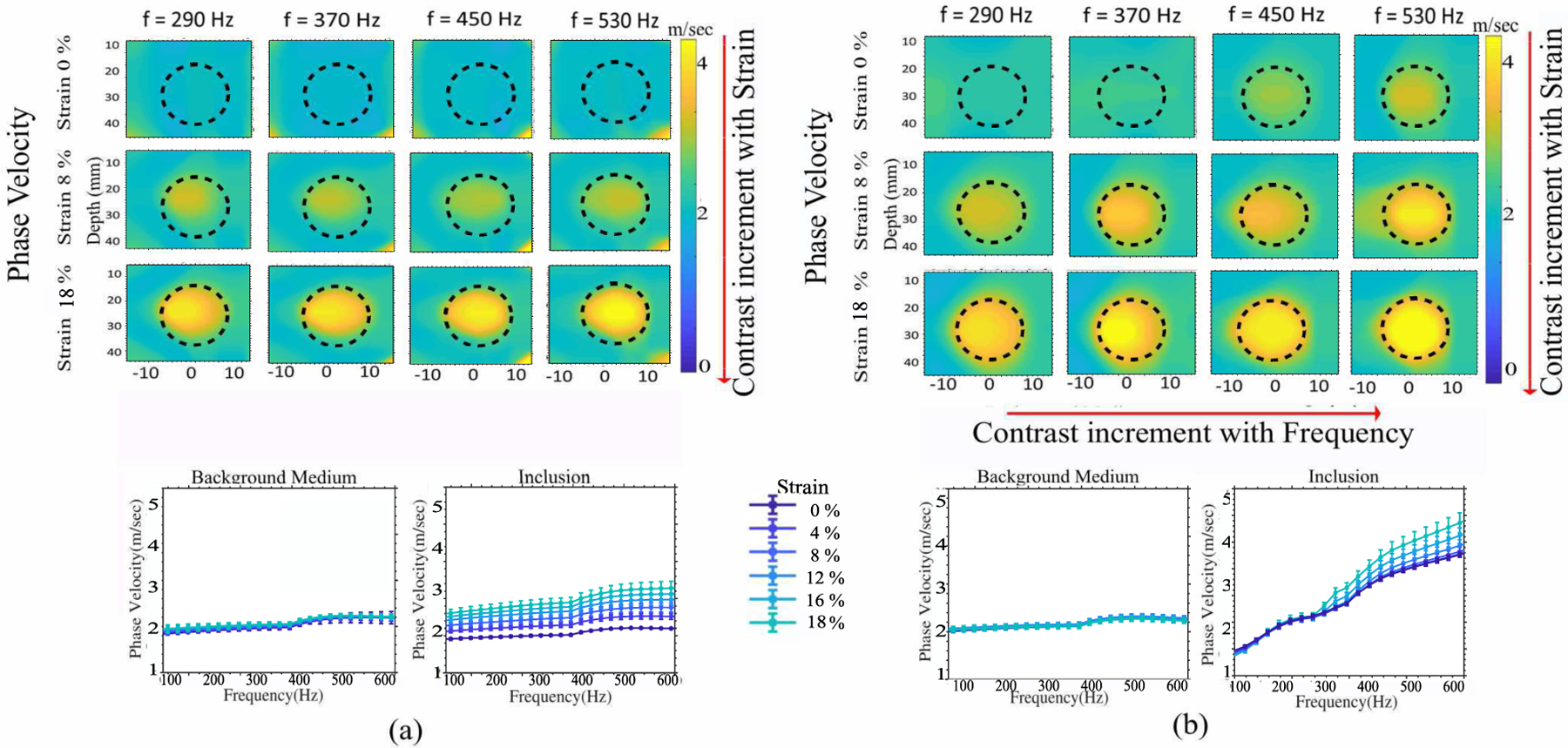
Contrast enhancement in simulated phase velocity images with higher nonlinearity and viscoelasticity of material. Representative simulated phase velocity images and quantitative plots of SWS vs frequency for (a) Nonlinear elastic inclusion-Linear Elastic medium (b) Nonlinear viscoelastic inclusion-Linear elastic medium. For (a) SWS increases with strain but consistent with frequency. For (b) SWS increases with frequency & strain.

Fig. 4 shows the three term hyperelastic parameters and the Voigt viscosity parameters used to simulate NLSM vs frequency. The solid line is the reference spectral NLSM curve based on simulation parameters. The shaded lines are reconstructed spectral NLSM by directly obtaining the simulated stress from COMSOL simulation and by estimating stress from the simulated SW velocity traces. The two homogeneous models show good agreement of reconstructed spectral NLSM with reference curves. The second homogeneous model has higher spectral NLSM than the first model owing to its higher nonlinearity and higher viscosity parameters. For the heterogeneous model with same model parameters as that of homogeneous one, the inclusion spectral NLSM reconstructed curve shows a higher deviation from the reference curve than the background. The reconstructed DSM and ESM simulated spectral NLSM show similar behavior as that of the reference NLSM curve from model parameters. From Fig. 4, we observe that the DSM spectral NLSM shows a deviation of 2–9% and 4–12 % from experimental values at 200 Hz and 500 Hz SW excitation frequency, respectively. The ESM simulated spectral NLSM shows deviation of 2–10% and 5–14% deviation at 200 Hz and 500 Hz frequency, respectively. Errors in estimation of shear modulus from SW traces result in higher deviation of ESM spectral NLSM from reference values.

Fig. 4.

Quantitative spectral NLSM plots showing reference NLSM vs frequency curve (solid lines) calculated based on model parameters and reconstructed curve through proposed approaches (DSM-direct stress obtained from simulation and ESM-estimated stress from simulated velocity traces). Two homogeneous models were simulated, and then a heterogeneous model with the same material parameters as that of the homogeneous ones (one for the background and one for inclusion) were simulated. The simulation models were generated with 18 % compound deformation comprising 18 % axial strain & 18% shearing.

1). Separate effect of elastic nonlinearity and viscosity on spectral NLSM:

Fig. 5 shows spectral NLSM simulated for three different homogeneous models. The first model has same nonlinearity as that of the second one but different viscosity. We observed a higher increase (15 % at 600 Hz ) in NLSM with frequency for the second model compared to the first one. This increment in spectral NLSM is due to effect of viscosity alone. The third model has different nonlinear parameters but has similar viscosity parameters. The third model shows a 16% higher increase in spectral NLSM compared to the second one. This is attributed to the effect of higher elastic nonlinearity of third model on spectral NLSM.

Fig. 5.

Quantitative NLSM vs frequency plots for three homogeneous models. The solid violet & black lines are reference curves based on simulation model parameters; and the blue & grey lines are curves reconstructed through proposed method with 18 % compound deformation for spectral NLSM and group SWS based NLSM, respectively. First model has same nonlinear hyperelastic parameter as that of second model but different viscosity. Second model has same viscosity that of third model but different nonlinearity. The second model has 15 % higher spectral NLSM at 600 Hz than the first model and this is due to the effect of viscosity difference on spectral NLSM. The third model has 16 % higher spectral NLSM than the second model owing to its higher elastic nonlinear parameters. Slope of NLSM vs frequency are 0.1 kPa/Hz, 0.158 kPa/Hz and 0.163 kPa/Hz for the three models respectively.

2). Strain effects on spectral NLSM reconstruction:

Here, we evaluate the effect of different types of deformations on spectral NLSM. Table. I shows spectral NLSM at four different SW frequencies for three different deformation types; compressional deformation (18 %), shearing deformation (18 %) and compound deformation (18 % axial compression and 18 % lateral shear). The reconstructed spectral NLSM has good correspondence for different strain types, with percent error from input values of 2.3–8.1%, 1.2–9%, 2–10.4% for compressional, shear, compound deformation types, respectively.

TABLE I.

Table represents simulated NLSM for different SW frequencies for different strain types. The strain types are compression strain (18%), shearing strain (18%) and compound deformation compression of 18 % and shearing 18 %. Model 1,2 and 3 are three models from Fig. 8 left to right. The reference NLSM vs frequency values can be found from Fig. 8

NLSM (kPa) vs SWS frequency for different strain types		200 Hz	300 Hz	400 Hz	500 Hz
Model 1	Compressional strain	123±8	129±7.2	143±9.8	149±10.4
	Shearing strain	124±6.5	126±6.9	134.8±7.7	142±8.4
	Compound deformation	116±9.6	123±9.3	136.4±11.3	146±15.1
	Reference model parameters	126	133	142	156
Model 2	Compressional strain	126.5±8.4	141±9.1	156.2±10.5	172±9.3
	Shearing strain	129±8	147±7.8	162±9	180±9.5
	Compound deformation	120±9.2	147±7.3	158±12	176±9.9
	Reference model parameters	134	150	170	187
Model 3	Compressional strain	147±10.3	177±11.9	189±13.4	205±14.5
	Shearing strain	151±7.8	182±9.5	193±11.1	209±11.5
	Compound deformation	150±11	175±12	191±13	206±15.3
	Reference model parameters	165	179	195	215

B. Experimental Results

1). Gelatin Phantoms:

Fig. 6 shows the representative B-mode, axial strain image, SWS, Group SWS-NLSM and frequency dependent NLSM for each of the three heterogeneous phantoms tested. Contrast Ratio (CR) was calculated and shown as a function of SW excitation frequency. The CR is given by $CR=20lo{g}_{10}\frac{{\mu }_I}{{\mu }_B}$, where μ_I and μ_B are the mean NLSM of the inclusion and the background, respectively. For quantitative analysis, both the background and inclusion ROI were chosen to be near the focal length [40] of the push beam. For the stiffer linear elastic inclusion in elastic background shown in Fig. 6(a), the group SWS based NLSM (SWS-NLSM) shows 6.5 dB higher contrast compared to linear SWS image, however both group SWS-NLSM and spectral NLSM shows relatively same CR of 12.5 dB. Phase velocity remains constant with SW excitation frequency and thus gives the same CR of 6 dB as that of SWS image. For the viscoelastic inclusion in elastic medium with similar initial SWS of 2.16 m/sec in Fig. 6(b), the linear SWS image and the group SWS based NLSM maps reconstruct the inclusion with poor contrast ( both around CR = 4 dB). This could be attributed to the fact that the group SWS based NLSM image does not consider the viscoelastic behavior of the material. Here, both the inclusion and surrounding medium have similar type of nonlinear behavior so the inlcusion is not well reconstructed in the group SWS-NLSM elastogram. The contrast of the inclusion in phase velocity images increases from 2 dB to 7.2 dB with SW excitation frequency. However, the contrast increment in spectral NLSM images is significantly higher, from 3 dB to 18.3 dB with increasing frequency. For the elastic inclusion in viscoelastic medium, the group SWS-NLSM gives 5 dB higher CR than the linear SWS image. Spectral NLSM images were obtainable up to a maximum of SW frequency of 450–500 Hz due to the increased SW attenuation of viscoelastic medium.

Fig. 6.

NLSM images as a function of SW frequency for different combinations of nonlinear viscoelastic inclusion gel phantoms. B-mode, axial strain image, linear SWS, Phase velocity, group SWS-NLSM, spectral NLSM images for (a) Elastic medium - Elastic inclusion (b) Elastic medium - Viscoelastic inclusion (c) Viscoelastic medium - Elastic inclusion phantoms. CR plots shown by taking rectangular and circular ROI’s shown in background and inclusion, respectively. The standard deviation was evaluated from 10 repeatable measurements. These experiments were performed under 18 % compound deformation comprising 18% compression and 18 % shearing. The experimental results are validated with reconstructed curves from model simulation parameters shown in dashed lines. The simulation model parameters were obtained by fitting a three term Ogden hyperelastic model to the cumulative stress-vs strain response as described in Section III B1.

2). Gel Phantom with Ex-vivo Liver Inclusion:

Fig. 7 presents the B-mode, axial strain image, linear SWS, group SWS based NLSM, spectral NLSM images and CR plots for three different small liver inclusion embedded in gelatin phantoms. The liver inclusion shows a spectral NLSM of 100–200 kPa at 150 Hz to 700–1600 kPa at 500 Hz SWS excitation frequency. The gelatin medium shows spectral NLSM of 40–60 kPa at 150 Hz to 100–150 kPa at 500 Hz frequency. This indicates that liver tissues are more nonlinear and viscoelastic compared to gelatin medium. For a liver inclusion of equal stiffness as that of gel medium in Fig. 7(a), the group SWS-NLSM shows 18 dB higher CR compared to linear SWS. Contrast of phase velocity images increases to 9.5 dB at 700 Hz SW excitation frequency. Spectral NLSM contrast rises to 36 dB at 700 Hz which is 10 dB higher than group SWS-NLSM image. The spectral NLSM of liver tissue rises to 1600 kPa compared to group SWS-NLSM of 760 kPa. For a liver inclusion in a softer viscoelastic gelatin medium illustrated in Fig. 7(b), the CR of spectral NLSM is 35 dB and 20 dB higher than phase velocity images and group SWS-NLSM images respectively. Furthermore, the CR of spectral NLSM in the liver-viscoelastic medium phantom is 17 dB higher than liver-elastic medium phantom in Fig. 7(a). For the liver inclusion in stiffer viscoelastic medium, the group SWS-NLSM of liver is higher than group SWS-NLSM of gelatin unlike the linear SWS. The phase velocity values are significantly higher in the liver tissue than the surrounding gelatin. Similar characteristics are observed for the spectral NLSM images with significantly higher contrast in spectral NLSM of liver tissue with frequency compared to gelatin.

Fig. 7.

NLSM image as a function of SW frequency, reconstructed for different combinations of liver inclusion surrounded by gelatin phantoms (a) Equal stiffness Liver inclusion in Elastic medium (b) Softer viscoelastic medium (c) Stiffer Viscoelastic medium. Quantitative NLSM and CR plots are shown by taking rectangular ROI in background and red-marked ROI in liver. The standard deviation was evaluated from 10 repeatable measurements. The experimental results are validated with reconstructed curves from model simulation parameters shown in dashed lines.The simulation model parameters were obtained by fitting A Ogden hyperelastic model to the cumulative stress-vs strain response as described in Section III B1.

3). Effect of Glutaraldehyde-treatment on Liver Tissue:

Fig. 8 show the effect in spectral NLSM with glutaraldehyde treatment. Prior to treatment, the gelatin medium has same linear SWS as liver tissue shown in Fig. 8(a). The group SWS-NLSM gives better contrast of liver tissue due to higher nonlinearity of liver, and the spectral NLSM further improves the contrast with frequency in Fig. 8(a). Following glutaraldehyde treatment, the linear SWS image in Fig. 8(b) shows higher SWS of liver, particularly, at the point of injection. The group SWS-NLSM also shows increased nonlinearity of the liver sample with glutaraldehyde treatment. The spectral NLSM images show marked increment in NLSM values following glutaraldehyde treatment increasing from of 850 kPa to 1370 kPa at 425 Hz. Exposure to glutaraldehyde results in a significant increase in stiffness of the tissue, thus increasing the elastic nonlinearity values. Moreover, the introduction of cross-links by glutaraldehyde creates resistance to the rearrangement of collagen in the applied stress direction, thus increasing viscous effect of the tissue [43].

Fig. 8.

Spectral NLSM images before (a) and after (b) glutaraldehyde treatment on liver inclusions. Position of glutaraldehyde treatment in the liver tissue is marked. Spectral NLSM images provide higher CR after glutaraldehyde treatment owing to increased nonlinearity and viscosity of liver tissue. Note, although we inject glutaraldehyde at two positions, it diffuses and we determined the ROI (red) by comparing SWS images before and after treatment.

4). Lateral resolution of spectral NLSM imaging:

We used the R₈₀₋₂₀ performance metric [45] to measure the lateral resolution in a transition region of heterogeneous medium, which was defined as R₈₀₋₂₀ = 2ln(4)w; where w is the width of the transition region. We estimated w by fitting a sigmoid function to the transition layer. The sigmoid curve was defined as $c(x)=c_2+\frac{c_1-c_2}{1+e^{\frac{x-x_1}{w}}}$ where c₁ and c₂ are SWS at two sides of the region and x₁ is the transition boundary. For a given SWS profile at a transition region, c₁, c₂, x₁, and w are estimated from nonlinear least squares fitting. Fig. 9 shows the effect of kernel (square window) length of strain and phase velocity estimation on lateral resolution of spectral NLSM imaging. Higher kernel length of strain and phase velocity estimation resulted in reduced lateral resolution.

Fig. 9.

(a) and (b) showing the lateral resolution of spectral NLSM imaging at two SW frequencies of 160 Hz and 430 Hz for different kernel (square window) length of strain and phase velocity estimation, respectively.

C. Spectral NLSM with freehand scan

Fig. 10 shows spectral NLSM images obtained by controlled compound deformation and freehand scanning in an oil-in gelatin inclusion embedded in gelatin medium phantom. While spectral NLSM images obtained by freehand scan shows distortion in the reconstruction of the inclusion, the mean spectral NLSM values have good correspondence with the NLSM values obtained by controlled deformation. The estimated standard deviation of NLSM measurements was 13–22 kPa with freehand scan compared to 6–12 kPa for controlled.

Fig. 10.

Spectral NLSM images with Controlled compound deformation and freehand scanning in an oil-in-gelatin inclusion in gelatin medium phantom. Quantitative spectral NLSM values of the inclusion for controlled deformation and freehand scan are shown (right side).

V. Discussion

In this study we present a new technique to concurrently image the tissue nonlinear elastic and viscoelastic properties locally, to aid in improved characterization of tissue biomechanics. Linear elasticity imaging alone does not provide a complete characterization as most biological tissues are nonlinear and viscoelastic. Nonlinear elasticity imaging has been difficult owing to the limitation of fixed controlled axial deformation needed to be given to the tissue. Linear viscoelasticity imaging has its own limitations because of the assumptions needed which are not well defined for tissue nonlinearity. Hence viscoelasticity and elastic nonlinearity cannot be decoupled and imaging of the two concurrently is more challenging. This study solves this problem by imaging the elastic nonlinearity (NLSM) as a function of SW excitation frequency at a local scale and with compound deformation. Effectively, we are studying the local effects of tissue viscoelasticity on nonlinear elastic properties. We did not study in this paper the effect of tissue nonlinearity on local higher order viscoelastic properties. This is a separate, interesting topic that was studied previously by Sinkus et al., however, their study was limited to a global scale. Similarly the effect of SW frequency dispersion on NLSM was studied by Otesteanu et al. that again was limited to global scale and uni-axial compression of the tissue. Our method of imaging local NLSM as a function of SW excitation frequency with compound deformation is more clinically realizable. Additionally, we observe increased contrast in elastograms due to concurrent evaluation of these parameters, rather than separate evaluation of them. Another observation, that, the spectral NLSM values are positive for the materials we used to make oil-in-gelatin phantoms and liver inclusion phantoms.

The inclusion phantom experiments from Figs. 6 and 7 show that spectral NLSM obtained for biological liver inclusions are significantly higher compared to linear elastic gel medium. This indicates higher nonlinearity and viscoelasticity of liver tissues compared to gelatin medium. The maximum SW frequency range captured by this spectral NLSM imaging method is limited for liver tissue to 450–500 Hz compared to 600–700 Hz for gelatin medium due to high frequency SW attenuation in the more viscous liver tissue. However, 450–500 Hz is large enough to capture the spectral NLSM behavior as illustrated in Fig. 7. Future studies would be directed towards incorporating the SW attenuation factor in the method to improve the maximum frequency range as well as the CNR of elastogram. The artifacts in spectral NLSM images in Fig. 7, particularly on the right hand side, could be attributed to the shear wave attenuation in both the viscous background medium and viscous liver inclusion. Our focused beam was on the left side of phantom, hence frequency dependent attenuation becomes more dominant with increase of distance from the source, distorting the shear-wave profile and introducing artifacts.

The spatial resolution of our spectral NLSM imaging method is determined by the spatial wavelengths (spatial kernel length) of the LPVI imaging, the spatial kernel used for the axial & lateral displacement estimation methods as shown in Fig. 9. High frequency (400–500 Hz) estimates of spectral NLSM are preferred as the shorter wavelength at higher frequency is suitable for resolving small inclusions (as indicated by higher resolution of spectral NLSM at 430 Hz than 160 Hz in Fig. 9).

Although the spectral NLSM images obtained by freehand scan in Fig. 10 show good agreement in mean NLSM values compared to that obtained by controlled deformation, the freehand scan elastograms are noiser. This could be attributed to the tracking errors due to the out-of-plane speckle decorrelation while giving freehand deformation. The time of total data acquisition needs to be reduced to limit the speckle de-correlation. The time of data acquisition mainly constitutes the SWEI acquisition time which could be reduced by a shorter push pulse and reduced angles of plane-wave compounding for SW tracking. However, shorter push duration reduces SNR of SWEI elastogram, which further affects reconstruction of phase velocity and spectral NLSM images. Future studies will be directed towards developing a fast integrated non-diffractive bessel beam based SWEI [42] and strain elastography acquisition scheme that captures more deformation level data rapidly, suitable for freehand spectral NLSM imaging. Feng et. al. [42] showed that bessel beam SWEI demonstrates improved depth of field, improved image quality with shorter push duration, accurate SWS estimates, and less energy usage. Furthermore, studies will be conducted towards spectral NLSM reconstruction with different random compound deformation types in in-vivo tissues.

This study proposes a novel dynamic shear wave based spectral NLSM simulation method. Previous studies were limited to static stress-strain simulation for NLSM imaging. The differences in SW propagation for different combinations of elastic, nonlinear elastic and nonlinear viscoelastic models with same group SWS are shown in Fig. 2. The NLSM estimation from simulated data were carried out in two ways; first, by directly using the apparent shear modulus from COMSOL (DSM) and second, by estimating the apparent shear modulus from simulated shear wave traces (ESM). The results obtained by both the proposed methods are in good agreement with the experimental spectral NLSM behavior and the reference spectral NLSM behavior obtained from simulated model parameters Fig. 3. However, the deviation increases with higher SW frequency as seen in Fig.3 and Fig. 5. This is because we are separately estimating the nonlinear elastic parameter by fitting the experimentally measured stress-strain behavior to the Ogden model and shear viscosity parameter by fitting the phase velocity as a function of SW frequency to the Voigt model. While fitting the phase velocity estimates to the Voigt model to obtain the setup shear viscosity for simulation, we used the phase velocity estimates at unstressed condition. However, we have also used experimental phase velocity estimates at highest strain of 18% to obtain shear viscosity. We observed that shear viscosity parameter does not change with deformation.

Exposure to glutaraldehyde increases both elastic nonlinearity and viscosity of liver tissue [43] as observed in spectral NLSM values of Fig. 8. In this study, we used large liver inclusion samples with 10 % glutaraldehyde treatment at the two positions of the liver inclusion as shown in Fig. 8(b). We restricted the amount of glutaraldehyde treatment to prevent its diffusion in the gelatin medium. By comparing the SWS image before and after glutaraldehyde treatment, we identified the treated zone by the red ROI (Fig. 8) and used for quantitative analysis. We also performed our spectral NLSM imaging method on whole liver tissue and obtained similar estimates as that of small liver samples in gelatin medium. Simulations of spectral NLSM with shearing deformation, compressional deformation and compound deformation show good agreement of spectral NLSM values (Table.I). Shearing deformation shows higher increment in simulated phase velocity with frequency and strain. Thus spectral NLSM can be obtained at lower shearing strain compared to compressional strain which will be studied in future.

VI. Conclusion

We have developed a novel frequency dependent nonlinear shear modulus imaging technique that concurrently images nonlinear elastic and viscoelastic behavior of tissues with compound deformation. Additionally, this imaging method provides improved contrast of the elastogram based on viscoelastic and nonlinear characterization compared to linear SWS imaging, phase velocity imaging and group SWS based NLSM imaging. Results from different combinations of linear elastic, nonlinear elastic and viscoelastic inclusion phantoms show that spectral NLSM magnitude increases with nonlinearity and viscosity of tissues. With this method we obtained maximum contrast ratio 32 dB, 25 dB, 34 dB and 25 dB higher than linear elasticity, group SWS-NLSM, phase velocity and strain imaging methods, respectively. Artificially cross-linked tissue showed enhanced spectral NLSM and nonlinear viscoelastic properties. Hence we can hypothesise that spectral NLSM properties are associated with degree of cross-linkage. Further clinical validation is required to demonstrate whether concurrent imaging of these properties might yield diagnostic information for lesion characterization.

REFERENCES

- [1].Nightingale K, McAleavey S and Trahey G, “Shear-wave generation using acoustic radiation force: In vivo and ex vivo results,” Ultrasound Med. Biol, vol. 29, no. 12, pp. 1715–1723,2003. [DOI] [PubMed] [Google Scholar]
- [2].McAleavey SA, Menon M, and Orszulak J, “Shear-modulus estimation by application of spatially-modulated impulsive acoustic radiation force,” Ultrasonic Imaging, vol. 29, no. 2, pp. 87–104,2007. [DOI] [PubMed] [Google Scholar]
- [3].Elegbe E, and McAleavey SA, “Single tracking location methods suppress speckle noise in shear wave velocity estimation,” Ultrasonic Imaging, vol. 35, no. 2, pp. 109–125,2013. [DOI] [PMC free article] [PubMed] [Google Scholar]
- [4].Ahmed R, Gerber S, McAleavey SA, Schifitto G, and Doyley M, “Plane wave imaging improves single track location shear wave elasticity imaging,” IEEE Trans. Ultrason., Ferroelectr., Freq. Control, vol. 65, no. 8, pp. 1402–1414, Aug. 2018. [DOI] [PMC free article] [PubMed] [Google Scholar]
- [5].Sickles EA, “The subtle and atypical mammographic features of invasive lobular carcinoma.” Radiology, vol. 178, no. 1, pp. 25–26, 1991. [DOI] [PubMed] [Google Scholar]
- [6].Arpino G, Bardou VJ, Clark GM, and Elledge RM, “Infiltrating lobular carcinoma of the breast: Tumor characteristics and clinical outcome,” Breast Cancer Res, vol. 6, no. 3, pp. 149–156, 2004. [DOI] [PMC free article] [PubMed] [Google Scholar]
- [7].Ricci P, Maggini E, Mancuso E, Lodise P, Cantisani V, and Catalano C, “Clinical application of breast elastography: state of the art.,” European journal of radiology, vol. 83, no. 3, pp. 429–437, 2014. [DOI] [PubMed] [Google Scholar]
- [8].Barry CT, Mills B, Hah Z, Mooney RA, Ryan CK, Rubens DJ, and Parker KJ, “Shear wave dispersion measures liver steatosis.,” Ultrasound in medicine & biology, vol. 38, no. 2, pp. 175–182, 2012. [DOI] [PMC free article] [PubMed] [Google Scholar]
- [9].Nightingale KR, Rouze NC, Rosenzweig SJ, Wang MH, Abdelmalek MF, Guy CD, and Palmeri ML. “Derivation and analysis of viscoelastic properties in human liver: impact of frequency on fibrosis and steatosis staging.,” IEEE transactions on ultrasonics, ferroelectrics, and frequency control, vol. 62, no. 1, pp. 165–175, 2015. [DOI] [PMC free article] [PubMed] [Google Scholar]
- [10].Brum J, Bernal M, Gennisson JL, and Tanter M, “In vivo evaluation of the elastic anisotropy of the human Achilles tendon using shear wave dispersion analysis.,” Physics in Medicine & Biology, vol. 59, no. 3, pp. 505, 2014. [DOI] [PubMed] [Google Scholar]
- [11].Rominger MB, Kälin P, Mastalerz M, Martini K, Klingmüller V, Sanabria S, and Frauenfelder T, “Influencing factors of 2D shear wave elastography of the muscle–an ex vivo animal study.,” Ultrasound international open, vol. 4, no. 2, pp. E54–E60, 2018. [DOI] [PMC free article] [PubMed] [Google Scholar]
- [12].Krouskop TA, Wheeler TM, Kallel F, Garra BS, and Hall T, “Elastic moduli of breast and prostate tissues under compression,” Ultrason. Imag, vol. 20, no. 4, pp. 260–274, 1998. [DOI] [PubMed] [Google Scholar]
- [13].Gennisson J-L, Catheline S, Bari C, Bercoff J, Tanter M, and Fink M, “Acoustoelasticity in soft solids: Assessment of the nonlinear shear modulus with the acoustic radiation force,” J. Acoust. Soc. Am, vol. 122 no. 6 pp. 3211–3219, 2007. [DOI] [PubMed] [Google Scholar]
- [14].Aristizabal S, Carrascal CA, Nenadic IZ, Greenleaf JF, and Urban MW, “Application of Acoustoelasticity to Evaluate Nonlinear Modulus inEx VivoKidneys,” IEEE transactions on ultrasonics, ferroelectrics, and frequency control, vol. 65, no. 2, pp 188–200, 2017. [DOI] [PMC free article] [PubMed] [Google Scholar]
- [15].Goswami S, Ahmed R, Doyley MM, and McAleavey SA, “Non-linear Shear Modulus Estimation with Bi-axial Motion Registered Local Strain,” IEEE Trans. Ultrason., Ferroelect., Freq. Control, vol. 66, no. 8, pp. 1292–1303, Aug. 2019. [DOI] [PMC free article] [PubMed] [Google Scholar]
- [16].Goswami S, Khan S, Ahmed R, Doyley MM, and McAleavey SA, “Deformation Independent Non-linearity Estimation: Studies and Implementation in Ultrasound Shear Wave Elastography,” 2019 IEEE International Ultrasonics Symposium (IUS), pp. 217–220. IEEE, 2019. [Google Scholar]
- [17].Goswami S, Ahmed R, Khan S, Doyley MM, and McAleavey SA. “Shear Induced Non-linear Elasticity Imaging: Elastography for Compound Deformations.”, IEEE Transactions on Medical Imaging, vol. 39, no. 11, pp. 3559–3570, 2020. [DOI] [PMC free article] [PubMed] [Google Scholar]
- [18].Bernal M, Chamming’s F, Couade M, Bercoff J, Tanter M, and Gennisson J-L, “In vivo quantification of the nonlinear shear modulus in breast lesions: Feasibility study,” IEEE Trans. Ultrason., Ferroelect., Freq. Control, vol. 63, no. 1, pp. 101–109, Jan. 2016. [DOI] [PubMed] [Google Scholar]
- [19].Insana MF, Pellot-Barakat C, Sridhar M, and Lindfors KK, “Viscoelastic imaging of breast tumor microenvironment with ultrasound.,” Journal of mammary gland biology and neoplasia, vol. 9, no. 4, pp. 393–404, 2004. [DOI] [PMC free article] [PubMed] [Google Scholar]
- [20].Bhatt M, AC Moussu M, Chayer B, Destrempes F, Gesnik M, Allard L, Tang A, and Cloutier G, “Reconstruction of viscosity maps in ultrasound shear wave elastography.,” IEEE Transactions on Ultrasonics, Ferroelectrics, and Frequency Control, vol. 66, no. 6, pp. 1065–1078, 2019. [DOI] [PubMed] [Google Scholar]
- [21].Hossain MM, and Gallippi CM, “Viscoelastic Response Ultrasound Derived Relative Elasticity and Relative Viscosity Reflect True Elasticity and Viscosity: In Silico and Experimental Demonstration.,” IEEE Transactions on Ultrasonics, Ferroelectrics, and Frequency Control, vol. 67, no. 6, pp. 1102–1117, 2019. [DOI] [PMC free article] [PubMed] [Google Scholar]
- [22].Kijanka P, and Urban MW, “Local phase velocity based imaging: A new technique used for ultrasound shear wave elastography.,” IEEE transactions on medical imaging, vol. 38, no. 4, pp. 894–908, 2018. [DOI] [PMC free article] [PubMed] [Google Scholar]
- [23].Rus G, Faris IH, Torres J, Callejas A, and Melchor J, “Why Are Viscosity and Nonlinearity Bound to Make an Impact in Clinical Elastographic Diagnosis?.,” Sensors, vol. 20, no. 8, pp. 2379, 2020. [DOI] [PMC free article] [PubMed] [Google Scholar]
- [24].Sinkus R, Bercoff J, Tanter M, Gennisson J, El Khoury C, Servois V, Tardivon A, and Fink M. “Nonlinear viscoelastic properties of tissue assessed by ultrasound.,” IEEE transactions on ultrasonics, ferroelectrics, and frequency control, vol. 53, no. 11, pp. 2009–2018, 2006. [DOI] [PubMed] [Google Scholar]
- [25].Otesteanu CF, Chintada BR, Rominger MB, Sanabria SJ, and Goksel O, “Spectral quantification of nonlinear elasticity using acoustoelasticity and shear-wave dispersion.,” IEEE transactions on ultrasonics, ferroelectrics, and frequency control, vol. 66, no. 12, pp. 1845–1855, 2019. [DOI] [PubMed] [Google Scholar]
- [26].Coussens LM and Werb Z, “Inflammation and cancer,” Nature, vol. 420, pp. 860–867, Dec. 2002. [DOI] [PMC free article] [PubMed] [Google Scholar]
- [27].Lipman SL, Rouze NC, Palmeri ML, and Nightingale KR, “Impact of acoustic radiation force excitation geometry on shear wave dispersion and attenuation estimates,” Ultrasound in medicine & biology, vol. 44, no. 4, pp. 897–908, 2018. [DOI] [PMC free article] [PubMed] [Google Scholar]
- [28].Montaldo G, Tanter M, Bercoff J, Benech N, and Fink M, “Coherent plane-wave compounding for very high frame rate ultrasonography and transient elastography,” IEEE Trans. Ultrason., Ferroelectr., Freq. Control, vol. 56, no. 3, pp. 489–506, 2009. [DOI] [PubMed] [Google Scholar]
- [29].Korshunov VA, Wang H, Ahmed R, Mickelsen DM, Zhou Q, Yan C, and Doyley MM, “Model-based vascular elastography improves the detection of flow-induced carotid artery remodeling in mice,” Scientific reports, Nature Publishing group, vol. 7, no. 1, PP. 12081, Feb. 2017. [DOI] [PMC free article] [PubMed] [Google Scholar]
- [30].Napoli ME, Freitas C, Goswami S, McAleavey S, Doyley M and Howard TM, “Hybrid Force/Velocity Control With Compliance Estimation via Strain Elastography for Robot Assisted Ultrasound Screening,” 7th IEEE International Conference on Biomedical Robotics and Biomechatronics (Biorob), Enschede, 2018, pp. 1266–1273. [Google Scholar]
- [31].Napoli ME, Goswami S, McAleavey SA, Doyley MM, and Howard TM, “Enabling quantitative robot-assisted compressional elastography via the extended Kalman filter,” Physics in Medicine & Biology, vol. 66, no. 22, pp. 225014, 2021. [DOI] [PubMed] [Google Scholar]
- [32].Napoli ME, Goswami S, McAleavey S, Doyley M, and Howard TM, “Probabilistic Mapping of Tissue Elasticity for Robot-Assisted Medical Ultrasound,” International Symposium on Robotics Research, Oct. 2019, forthcoming. [Google Scholar]
- [33].Rao M, Varghese T, and Madsen EL, “Shear strain imaging using shear deformations,” Medical physics vol 35, no. 2, pp. 412–423, 2008. [DOI] [PMC free article] [PubMed] [Google Scholar]
- [34].Ahmed R, and Doyley MM, “Distributing Synthetic Focusing Over Multiple Push-Detect Events Enhances Shear Wave Elasticity Imaging Performance,” IEEE transactions on ultrasonics, ferroelectrics, and frequency control, vol. 66, no. 7, pp.1170–1184, 2019. [DOI] [PMC free article] [PubMed] [Google Scholar]
- [35].Loupas T, Powers J, and Gill RW, “An axial velocity estimator for ultrasound blood flow imaging based on a full evaluation of the Doppler equation by means of a two-dimensional autocorrelation approach,” IEEE Trans. Ultrason. Ferroelectr. Freq. Control, vol. 42 no. 4, pp. 672–688, 1995. [Google Scholar]
- [36].Lipman SL, Rouze NC, Palmeri ML, and Nightingale KR, “Evaluating the improvement in shear wave speed image quality using multidimensional directional filters in the presence of reflection artifacts,” IEEE Trans. Ultrason. Ferroelectr. Freq. Control, vol. 63 no. 8, pp.1049–1063, 2016. [DOI] [PMC free article] [PubMed] [Google Scholar]
- [37].Jensen JA, “Field: A Program for Simulating Ultrasound Systems,” 10th Nordic-Baltic Conference on Biomedical Imaging, pp. 351–353, Vol. 34, Supplement 1, Part 1, 1996. [Google Scholar]
- [38].Ogden RW, “Non-Linear Elastic Deformations,” Courier Corporation, 1997. [Google Scholar]
- [39].Kim B, Lee SB, Lee J, et al. , “A comparison among Neo-Hookean model, Mooney-Rivlin model, and Ogden model for chloroprene rubber.,” Int. J. Precis. Eng. Manuf, vol. 13, pp. 759–764, 2012. [Google Scholar]
- [40].Lu J, Zou H, and Greenleaf J, “Biomedical Ultrasound Beam Forming.,” Ultrasound Med. Biol, vol. 20, pp. 403–428, 1994. [DOI] [PubMed] [Google Scholar]
- [41].Parker KJ, Szabo T, and Holm S, “Towards a consensus on rheological models for elastography in soft tissues.,” Physics in Medicine & Biology, vol. 64, no. 21, pp.215012, 2019. [DOI] [PMC free article] [PubMed] [Google Scholar]
- [42].Feng F, Goswami S, Khan S, and McAleavey SA, “Shear Wave Elasticity Imaging Using Nondiffractive Bessel Apodized Acoustic Radiation Force.,” IEEE Transactions on Ultrasonics, Ferroelectrics, and Frequency Control, July 8, 2021. [DOI] [PMC free article] [PubMed] [Google Scholar]
- [43].Van Noort R, Yates SP, Martin TRP, Barker AT, and Black MM, “A study of the effects of glutaraldehyde and formaldehyde on the mechanical behaviour of bovine pericardium.,” Biomaterials, vol. 3, no. 1, pp. 21–26, 1982. [DOI] [PubMed] [Google Scholar]
- [44].Goswami S, Ahmed R, Doyley MM, and McAleavey SA, “Quantitative nonlinear shear modulus mapping using freehand scanning.,” IEEE International Ultrasonics Symposium (IUS), pp. 1–3. IEEE, 2020. [Google Scholar]
- [45].Rouze NC, Wang MH, Palmeri ML, and Nightingale KR, “Parameters affecting the resolution and accuracy of 2-D quantitative shear wave images.,” IEEE transactions on ultrasonics, ferroelectrics, and frequency control, vol. 59, no. 8, pp.1729–1740, 2012. [DOI] [PMC free article] [PubMed] [Google Scholar]