A large-scale neural network training framework for generalized estimation of single-trial population dynamics

Abstract

Achieving state-of-the-art performance with deep neural population dynamics models requires extensive hyperparameter tuning for each new dataset. AutoLFADS is a model-tuning framework that produces high-performing autoencoding models on data from a variety of brain areas and tasks, automatically, without behavioral or task information. We demonstrate its broad applicability via an array of rhesus macaque datasets: motor cortex during free-paced reaching, somatosensory cortex during reaching with perturbations, and dorsomedial frontal cortex during a cognitive timing task.

Ongoing advances in neural interfacing technologies allow the activity of large neural populations to be monitored, across a wide variety of brain areas and behaviors (1–5). Several approaches have been developed to infer underlying latent dynamical neural structure from this activity on individual trials, including a growing number that leverage artificial neural networks (ANNs) (6–11). One particularly successful method, latent factor analysis via dynamical systems (LFADS), is a sequential variational autoencoder (SVAE) that uses recurrent neural networks (RNNs) to model neuronal population dynamics. ANN models like LFADS can be difficult to optimize because they generally require thorough hyperparameter (HP) tuning to achieve good performance. High-performing LFADS models are typically identified through evaluation with behavioral data, which further complicates optimization when behavioral correlates are limited (e.g., in cognitive areas). Here we present AutoLFADS, an unsupervised framework for automated model tuning that enables accurate single-trial inference of neural population dynamics across a range of brain areas and behaviors. Because it does not require behavioral correlates as labels, AutoLFADS avoids introducing representational biases and enables dynamical modeling of neural data lacking explicit behavioral correlates. We demonstrate that AutoLFADS provides improved representations of neural activity for rhesus macaque datasets spanning motor, somatosensory, and cognitive areas during a variety of tasks.

Enabling robust hyperparameter tuning for LFADS

The LFADS architecture (Fig. 1a and Methods) has been detailed previously (8,10,12). LFADS is an SVAE that approximates the latent dynamical system underlying observed neural population activity using an RNN (the “Generator”). It treats sequences of binned spike counts as noisy observations of an underlying Poisson process. Given an observed sequence, the model infers an underlying firing rate for each neuron at each time step. The training objective maximizes a lower bound on the marginal likelihood of the observed spiking activity, given the inferred rates (see Methods for details).

Figure 1 |. Combining a novel regularization technique with a large-scale framework for automated HP optimization.

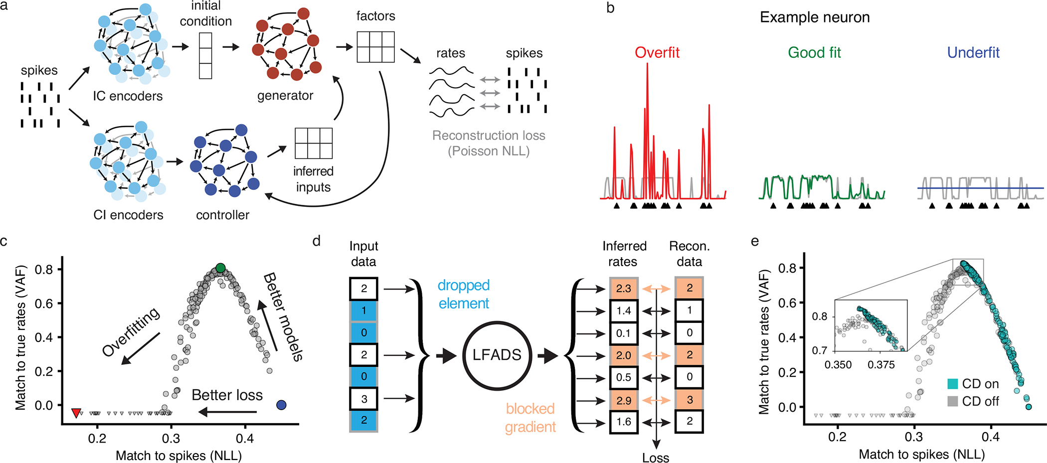
(a) The LFADS architecture, which infers the firing rates that underlie observed spikes. (b) Examples of LFADS-inferred rates (colored), the corresponding synthetic input data (spikes, shown as black triangles), and the data-generating distribution (ground truth rates, shown as gray traces) for three models of differing quality. (c) Performance of 200 LFADS models with random HPs for a synthetic dataset. Performance is computed via two metrics: how well the models match spikes (i.e., validation negative log-likelihood; NLL) and how well they match the synthetic firing rates that generated the spikes (i.e., variance accounted for; VAF). Gray points indicate random search models and colored points indicate the models that produced the rates in the previous panel. Triangles indicate models with negative VAF. All metrics were computed on validation data. (d) Schematic of coordinated dropout (CD) regularization. Random elements of the input data tensor are zeroed and the rest are scaled up, as in the standard dropout layer. Loss gradients are blocked for these elements to prevent overfitting to spikes (indicated with colored arrows). (e) Same as in (c), but including models trained with CD.

It is imperative to train and regularize the model properly for accurate inference of firing rates (Fig. 1b) (12). This can be achieved through optimization of a variety of hyperparameters (e.g., scaling factors for KL and L2 penalties, dropout probability, and learning rate, all described in Methods). The optimal values of these HPs could depend on various factors, including the dataset size, the dynamical structure of the relevant brain area, and the behavioral task.

A critical challenge to proper training and regularization of high-capacity SVAEs on spiking neural data is that their recognition models may allow them to find trivial solutions that simply pass individual spikes from input to output, akin to an identity transformation of the input, without modeling any meaningful structure underlying the data (Fig. 1b, left). Importantly, this failure mode cannot be detected via the standard validation metric, i.e., evaluating validation loss on held-out trials, because the identity-like transformation performs similarly on training and validation data. We term this failure mode “identity overfitting” and distinguish it from the standard notion of overfitting to training data. We demonstrated identity overfitting using a synthetic dataset with known firing rates (Fig. 1c; see Methods). As shown, models that appear to have the best likelihoods actually exhibit poor inference of underlying firing rates.

The lack of a reliable validation metric has prevented automated HP searches because it is unclear how one should select between models when underlying firing rates are unavailable or non-existent. While comparing likelihoods for data seen and not seen by the encoders (e.g. via co-smoothing (13) or sample validation (12)) may give some indication of the degree of identity overfitting, these metrics alone are insufficient for model selection because they don’t measure identity overfitting to heldin neurons. To address this issue we developed a novel regularization technique, coordinated dropout (CD), that prevents identity overfitting altogether (12). At each training step, standard dropout is applied to the input data elements (i.e., spike count bins). At the model’s output, where reconstruction loss is computed, the complement of the dropout mask is used to block gradient flow corresponding to reconstruction of data elements that were kept at the input (Fig. 1d). This strategy effectively prevents the network from learning an identity transformation because individual data elements cannot be used for self-reconstruction. Note that since CD is a regularization strategy, it is only applied during model training. By preventing identity overfitting, CD restores the correspondence between validation likelihood and rate reconstruction, rendering likelihood a suitable metric for model selection (Fig. 1e). Summary metrics for these and all subsequent analyses are aggregated in Supp. Table 1.

Our regularization strategy enables large-scale HP searches and unsupervised, fully-automated selection of high-performing autoencoders on real neuroscientific data, despite having no access to ground truth firing rates. To tune HPs, we use Population-based Training (PBT; Extended Data Figure 1a), which distributes training over dozens of workers simultaneously and uses evolutionary algorithms to adjust HPs dynamically over the course of training (14,15). PBT matches the scalability of parallel search methods like random or grid search, while achieving higher performance with the same compute cost in our tests (Extended Data Figure 1b). PBT also enables discovery of dynamic HP tuning schedules and allows exploration outside the search initialization ranges (Extended Data Figure 1c).

Outperforming LFADS on benchmark data

We first evaluated AutoLFADS on the “maze” delayed-reaching dataset used to develop and assess the original LFADS method (8,16). This dataset consisted of recordings from primary motor (M1) and dorsal premotor (PMd) cortex as a monkey made a variety of straight and curved reaches following target presentation and a delay period (Fig. 2a). The dataset contained multiple highly stereotyped trials per condition.

Figure 2 |. Applying AutoLFADS to four diverse datasets.

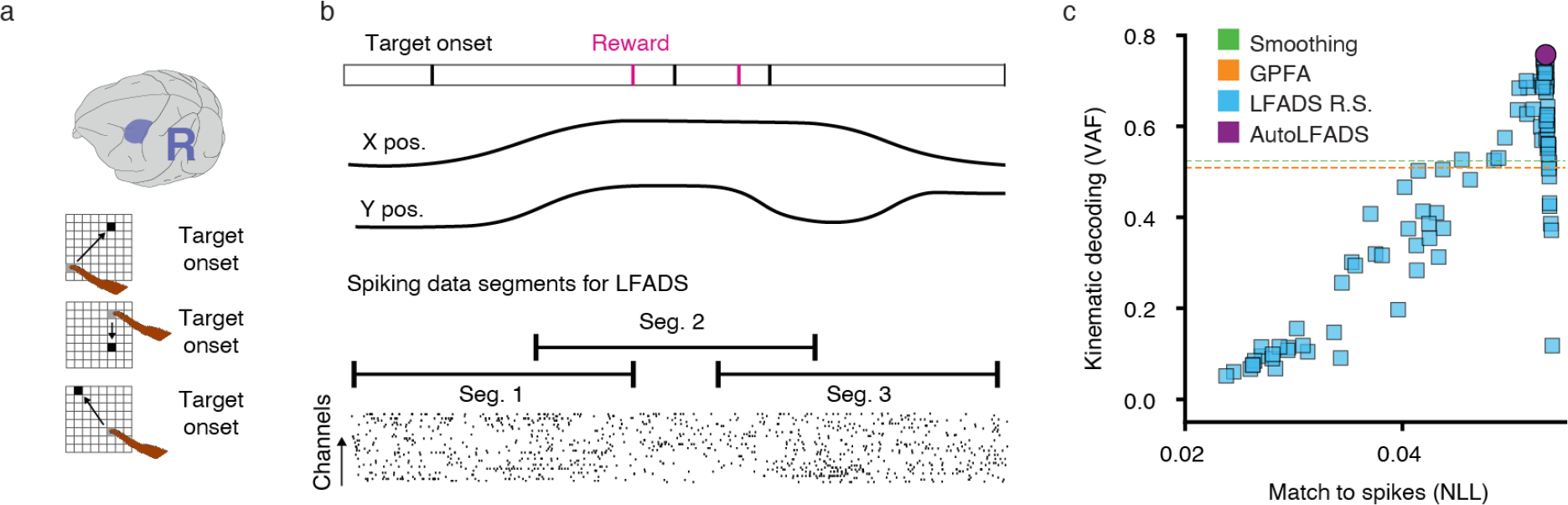
(a) Brain area and task schematics for the motor cortex maze dataset, MM. (b) Hand velocity decoding performance (VAF, mean of x- and y-directions) from firing rates as a function of training dataset size for AutoLFADS in comparison to smoothing and LFADS M.T (manually tuned) baselines. Lines and shading denote mean +/− standard error across 7 models trained on randomly-drawn trial subsets. (c) Same as (a), for the motor cortex random target dataset, MR. (d) Top three principal components of neural activity on single trials colored by angle to the target. (e) Hand velocity decoding performance for AutoLFADS in the random target task in comparison to smoothing, GPFA, and LFADS R.S. (random search) baselines. For LFADS R.S., error bars denote upper and lower quartiles (N=100). (f) Same as (a), for the area 2 dataset, A. (g) Joint angular velocity decoding performance from firing rates inferred using smoothing, GPFA, and AutoLFADS. Bars indicate mean and error is standard error of the mean across cross-validation splits (N=5). Joint abbreviations: shoulder adduction (SA), shoulder rotation (SR), shoulder flexion (SF), elbow flexion (EF), wrist radial pronation (RP), wrist flexion (WF), and wrist adduction (WA). (h) Same as (a), for the DMFC dataset, D. (i) PSTHs for an example neuron during the Set-Go period of rightward trials for two response modalities and all values of t_s. Vertical scale bars denote spikes / sec. (j) Distributions of correlation coefficients across 40 different task conditions. Horizontal lines denote medians. For LFADS, the distribution includes correlation values for all 96 models with random HPs (40×96 values). (k) Comparison between performance of AutoLFADS and random search on a 184-trial subset, as measured by two supervised metrics (kinematic decoding and PSTH reconstruction). Arrows indicate direction of better performance for each metric. (l) Same as (k), for the full area 2 dataset (decoding from active trials only). (m) Same as (k), for the full DMFC dataset. The kinematic decoding metric is replaced by the correlation between neural speed and the produced interval.

As shown in previous applications of LFADS on this dataset (8,12), the firing rates inferred by AutoLFADS had a consistent structure across trials (Extended Data Figure 2a) that captured features of the smoothed and trial-averaged neural responses (Extended Data Figure 3b).

While manually-tuned LFADS models and AutoLFADS models inferred rates with similar hand-velocity decoding accuracy when trained on the full 1836-trial training set (Fig. 2b), most neuroscientific datasets consist of far fewer trials. To simulate this scenario, we trained models on subsets of trials and found that AutoLFADS significantly outperformed manual tuning on the small datasets (Fig. 2b; p<0.05 for all three sizes, paired, one-tailed Student’s t-test).

Modeling population dynamics without structured trials

To-date, most experiments that tie dynamics to neural computations have used constrained tasks and repeated, highly structured trials. However, such paradigms may not be good proxies for everyday behaviors and may impose artificial limits on the properties of the uncovered dynamics (17). To address these limitations, we applied AutoLFADS to neural activity from a monkey performing a continuous, self-paced random target reaching task (Fig. 2c), in which each movement started and ended at a random position (18). Analysis of data without consistent temporal structure across trials is challenging, as trial-averaging is not feasible. Further, the strong simplifying assumptions that are typically used for single-trial analyses - for example, that the arm is in a consistent starting point, and that data windows are aligned to behavioral events such as target or movement onset (7,11,12,19–23) - are not applicable when analyzing less structured tasks.

Since typical fixed-length, trial-aligned data segments were not an option for this dataset, we divided the data into overlapping segments without regard to trial boundaries (Extended Data Figure 4b). After modeling with AutoLFADS, we merged inferred firing rates from individual segments into a continuous window, using a weighted combination of rates at overlapping time points. We then analyzed the inferred rates by aligning the data to movement onset for each trial (see Methods). Even though the dataset was modeled without the use of trial information, inferred firing rates during reconstructed trials exhibited consistent progression in an underlying state space, with clear structure that corresponded with the monkey’s reach direction on each trial (Fig 2d). Again, we demonstrate that AutoLFADS outperforms a random search in hand velocity decoding (Fig. 2e and Extended Data Figure 4c). Further, we show that AutoLFADS learns to infer rates that clearly reveal velocity, position, and target subspaces without any information about task structure (Supp. Note 1 and Supp. Fig. 1).

Modeling population dynamics in somatosensory cortex

Brodmann’s area 2 of somatosensory cortex (area 2) provides a valuable test case for generalization of AutoLFADS to more strongly input-driven brain areas. Area 2 receives afferent input from both cutaneous and muscle receptors and is robustly driven by mechanical perturbations to the arm (19,24,25). We applied AutoLFADS to recordings made during active (reaching) and passive (perturbations) arm movements in eight directions (Fig. 2f).

The single-trial rates inferred by AutoLFADS for passive trials exhibited clear and structured responses to the unpredictable perturbations (Extended Data Figure 2c), highlighting the model’s ability to approximate input-driven dynamics. The inferred rates also had a close correspondence to PSTHs aligned to movement onset during both types of trials (Extended Data Figure 5c). Additionally, the inferred inputs revealed structure corresponding to trials, directions, and perturbation types (Supp. Note 2, Supp. Fig. 2, & Supp. Video 1).

Sensory brain regions like area 2 are typically characterized in terms of how neural activity encodes sensory stimuli (19,24,25). For the vast majority of neurons across two datasets, AutoLFADS rates achieved better likelihoods on binned spike counts than generalized linear models (GLMs) based on hand position, hand velocity, and force applied to the handle (Extended Data Figure 5b; p<0.05 for 110/121 neurons, bootstrap; see Methods). This indicates that representations inferred by AutoLFADS go beyond simple kinematics and could provide insight into the computational dynamics of area 2. Example GLM predictions are shown in Extended Data Figure 5c.

The AutoLFADS rates formed subspaces that represented hand velocity more clearly than smoothed spikes, for both active and passive movements and across all conditions (Extended Data Figure 5d). On a second dataset that included whole-arm motion tracking, joint angle velocity decoding from AutoLFADS rates was more accurate than from rates obtained by smoothing or GPFA (Fig. 2g; p<0.05 for all joints, paired, one-sided Student’s t-Test).

Modeling cognitive population dynamics in frontal cortex

We further tested the generality of AutoLFADS by applying it to data collected from dorsomedial frontal cortex (DMFC) as a macaque attempted to reproduce a given time interval (t_s) by waiting (t_p) before initiating a response movement (Fig. 2h; see Methods) (26). The task requires both sensory input processing and internal timing and includes 40 task conditions—10 intervals (t_s), two response modalities (joystick and saccade), and two target locations (left and right). Population dynamics in DMFC are tied to behavioral correlates such as the movement production time, t_p (26–28).

AutoLFADS rates for this dataset showed consistent, denoised structure at the single-trial level (Extended Data Figure 2e). Notably, AutoLFADS captured the t_s-dependent ordering of PSTHs observed in previous work for both response modalities (Fig. 2i and Extended Data Figure 6b) (26). We found similar results in a qualitative characterization of AutoLFADS latent factors (Supp. Note 3 and Supp. Fig. 3).

Previous studies used PSTHs to show that, on average, the speed at which neural trajectories evolve during the waiting interval is negatively correlated with the time to initiate a response (t_p) (26,27). Using AutoLFADS, we found that this correspondence held for single trials: speed computed from AutoLFADS rates was more strongly correlated with t_p on a single trial basis than speed computed from rates obtained by smoothing, GPFA, and LFADS random search. We show results for individual trials across two timing conditions (Extended Data Figure 6c) and summarize across all 40 task conditions (Fig. 2j and Extended Data Figure 6d). Correlations from rates inferred by AutoLFADS were significantly better than all unsupervised approaches and comparable with supervised model selection, despite using no task information.

Comparison to supervised model selection

A significant drawback of supervised model selection is that it’s unclear whether models selected using one criterion will also be high-performing with respect to other criteria. We evaluated AutoLFADS models and LFADS random searches using supervised performance metrics across a 184-trial maze subset (Fig. 2k, Extended Data Figures 2b and 3c), the area 2 dataset (Fig. 2l and Extended Data Figures 2d and 5e), and the DMFC dataset (Fig. 2m and Extended Data Figure 2f and 6d). For random search models, the metrics often show substantial disagreement over which models are highest-performing. As a result, supervised model selection can introduce bias to the resulting rates. For example, selecting a random search model based on kinematic decoding for area 2 would result in suboptimal PSTH reconstruction and vice-versa. On the other hand, AutoLFADS models learn representations that perform as well as or better than the best random search models across all of our supervision metrics.

Discussion

The original LFADS work (8) provided a method for inferring latent dynamics, underlying firing rates, and external inputs from the activity of large populations of neurons, producing representations that were more informative of behavior than previous approaches (29). However, application to datasets with unpredictable external inputs, complex neural population dynamics, or unconstrained behavior required time-consuming and subjective manual tuning. This process was further complicated by identity overfitting, which made supervised model selection necessary for systematic HP optimization. This could be achieved by (1) decoding an external behavioral variable from inferred rates or (2) comparing inferred rates to empirical PSTHs. The first option required measured behavioral data, biased evaluation toward representational hypotheses, and only evaluated a handful of potentially low-variance dimensions in the population activity. The second required structured tasks with repeated trials, relied on hand-tuned parameters like smoothing width, and biased evaluation towards trial-averaged responses.

In the current work, we show that AutoLFADS enables training of high-performing LFADS models in an unsupervised fashion for neural spiking datasets of arbitrary size, trial structure, and dynamical complexity. This was achieved by combining a novel regularization technique and efficient hyperparameter tuning. Critically, AutoLFADS is both less restrictive and higher performing than the aforementioned supervised evaluation approaches. It does not require repeated trials or behavioral variables for model selection, yet consistently outperforms models selected via the same supervised criteria.

We demonstrated several other properties of AutoLFADS that have broad implications. On the maze task, we showed that AutoLFADS models are more robust to dataset size, opening up new lines of inquiry on smaller datasets and reducing the number of trials that must be conducted in future experiments. Using the random target task, we demonstrated that AutoLFADS needs no task information in order to generate rich dynamical models of neural activity. This enables the study of dynamics during richer tasks and reuse of datasets collected for other purposes. With the perturbed reaching task, we demonstrated for the first time the application of dynamical modeling to the highly input-driven somatosensory cortex. Finally, in the timing task we showed that AutoLFADS revealed single-trial representations for neural data without overt behavioral correlates, opening the door to new applications in cognitive areas. It is worth noting that in all the above scenarios, AutoLFADS models matched or outperformed the best LFADS models in terms of behavioral metrics, despite not using any behavioral information during training or model selection. Some comparisons to other methods are already available in the recently introduced Neural Latents Benchmark (see AutoLFADS metrics in Supp. Table 2), and more are forthcoming (13). We provide further information on running AutoLFADS in the cloud and extending PBT in Supp. Note 4 and more flexible deployment strategies for ad-hoc and managed computing clusters are under development (30).

AutoLFADS inherits some basic assumptions of LFADS—for example, the linear-exponential-Poisson observation model, which is likely an oversimplification. We used this architecture as a starting point to show that a large-scale hyperparameter search is feasible and beneficial, but recent applications to EMG and calcium imaging data demonstrate that AutoLFADS is reasonably straightforward to extend (31–33). By enabling large-scale searches, we can be reasonably confident that any performance benefits achieved by future architecture changes are due to real differences in modeling capabilities rather than a lack of HP optimization. AutoLFADS does still require the user to select HP ranges for initialization, but these ranges are more relevant to optimization speed than to final performance, as evolutionary algorithms guide HP trajectories outside of the initialization ranges if this leads to higher-performing models. If the user has no prior for reasonable search ranges, we recommend using a large initialization range at the risk of requiring more compute time.

Taken together, these results show that AutoLFADS provides an extensible framework for inference of single-trial neural dynamics with unprecedented accuracy. Its accessibility and generality allows a single framework to be used to study computation through dynamics across brain areas and tasks.

Methods

Non-human primates

Our research complies with all relevant ethical regulations. The studies that collected the data were approved by Institutional Animal Care and Use Committees at Stanford University (maze dataset), UCSF (random target dataset), Northwestern University (area 2 dataset), and MIT (DMFC dataset). For more information about the animals used in those experiments, please see publications where the relevant data were originally published (16,18,19,26).

LFADS architecture and training

A detailed overview of the LFADS model is given in (8). Briefly: at the input to the model, a pair of bidirectional RNN encoders read over the spike sequence and produce initial conditions for the generator RNN and time-varying inputs for the controller RNN. All RNNs were implemented using gated recurrent unit (GRU) cells. The first generator state is computed with a linear mapping from the initial condition, such that the dimensionality of the inferred initial conditions is not constrained to be the same as the number of units in the generator RNN. At each time step, the generator state evolves with input from the controller and the controller receives delayed feedback from the generator. The generator states are linearly mapped to factors, which are mapped to the firing rates of the original neurons using a linear mapping followed by an exponential. The optimization objective is to minimize the negative log-likelihood of the data given the inferred firing rates, and includes KL and L2 regularization penalties.

Identical architecture and training hyperparameter values were used for most runs, with a few deviations. We used a generator dimension of 100, initial condition dimension of 100 (50 for area 2 runs), initial condition encoder dimension of 100, factor dimension of 40, controller and controller input encoder dimension of 80 (64 for DMFC runs), and controller output dimension of 4 (10 for overfitting runs).

We used the Adam optimizer with an initial learning rate of 0.01 and, for non-AutoLFADS runs, decayed the learning rate by a factor of 0.95 after every 6 consecutive epochs with no improvement to the validation loss. Training was halted for these runs when the learning rate reached 1e-5. The loss was scaled by a factor of 1e4 immediately before optimization for numerical stability. GRU cell hidden states were clipped at 5 and the global gradient norm was clipped at 200 to avoid occasional pathological training.

We used a trainable mean initialized to 0 and fixed variance of 0.1 for the Gaussian initial condition prior and set a minimum allowable variance of 1e-4 for the initial condition posterior. The controller output prior was autoregressive with a trainable autocorrelation tau and noise variance, initialized to 10 and 0.1, respectively.

Memory usage for RNNs is highly dependent on the sequence length, so batch size was varied accordingly (100 for maze and random target datasets, 500 for synthetic and area 2 datasets, and 300/400 for the DMFC dataset). KL and L2 regularization penalties were linearly ramped to their full weight during the first 80 epochs for most runs to avoid local minima induced by high initial regularization penalties. Exceptions were the runs on synthetic data, which were ramped over 70 epochs and random searches on area 2 and DMFC datasets, which used step-wise ramping over the first 400 steps.

Random searches and AutoLFADS runs used the architecture parameters described above, along with regularization HPs sampled from ranges (or initialized with constant values) given in Supp. Table 4 and Supp. Table 5. Most runs used a default set of ranges, with a few exceptions outlined in the table. Dropout was sampled from a uniform distribution and KL and L2 weight HPs were sampled from log-uniform distributions. In general, more coservative hyper-HP settings (e.g., low learning rates and very wide initialization and search ranges) will work consistently across datasets. This approach is recommended in general, but as the experimenter becomes familiar with training AutoLFADS on the dataset, they may want to improve optimization speed by limiting exploration to relevant parts of the HP space.

During PBT, weights were used to control maximum and minimum perturbation magnitudes for different HPs (e.g. a weight of 0.3 results in perturbation factors between 0.7 and 1.3). The dropout and CD HPs used a weight of 0.3 and KL and L2 penalty HPs used a weight of 0.8. CD rate, dropout rate, and learning rate were limited to their specified ranges, while the KL and L2 penalties could be perturbed outside of the initial ranges. Each generation of PBT consisted of 50 training epochs. AutoLFADS training was stopped when the best smoothed validation NLL improved by less than 0.05% over the course of four generations.

Validation NLL was exponentially smoothed with α = 0.7 during training. For non-AutoLFADS runs, the model α = 0. 7 checkpoint with the lowest smoothed validation NLL was used for inference. For AutoLFADS runs, the checkpoint with the lowest smoothed validation NLL in the last epoch of any generation was used for inference. Firing rates were inferred 50 times for each model using different samples from initial condition and controller output posteriors. These estimates were then averaged, resulting in the final inferred rates for each model.

Overfitting on synthetic data

Synthetic data were generated using a 2-input chaotic vanilla RNN (γ = 1.5) as described in the original LFADS work (8, 10). The only modification was that the inputs were white Gaussian noise. In brief, the 50-unit RNN was run for 1 second (100 time steps) starting from 400 different initial conditions to generate ground-truth Poisson rates for each condition. These distributions were sampled 10 times for each condition, resulting in 4000 spiking trials. Of these trials, 80% (3200 trials) were used for LFADS training and the final 20% (800 trials) were used for validation. Detailed parameters for all datasets used in the paper can be found in Supp. Table 3.

We sampled 200 HP combinations from the distributions specified in Supp. Table 4 and used them to train LFADS models on the synthetic dataset. We then trained 200 additional models with the same set of HPs using a CD rate of 0.3 (i.e., using 70% of data as input and remaining 30% for likelihood evaluation) (12). The coefficient of determination between inferred and ground truth rates was computed across all samples and neurons on the 800-sample validation set.

M1 maze task

We used the previously-collected maze dataset (16) described in detail in the original LFADS work (8). Briefly, a male macaque monkey performed a two-dimensional center-out reaching task by guiding a cursor to a target without touching any virtual barriers while neural activity was recorded via two 92-electrode arrays implanted into M1 and dorsal PMd. The full dataset, collected from Jenkins on September 18th, 2009, consisted of 2,296 trials, 108 reach conditions, and 202 single units.

The spiking data were binned at 1 ms and smoothed by convolution with a Gaussian kernel (30 ms s.d.). Hand velocities were computed using second order accurate central differences from hand position at 1kHz. An antialiasing filter was applied to hand velocities and all data were then resampled to 2 ms. Trials were created by aligning the data to 250 ms before and 450 ms after movement onset, as calculated in the original paper.

Datasets of varying sizes were created for LFADS by randomly selecting trials with 20, 10, and 5% of the original dataset using seven fixed seeds, and then splitting each of these into 80/20 training and validation sets for LFADS (22 total, including the full dataset). As a baseline for each data subset, we trained LFADS models with fixed HPs that had been previously found to result in high-performing models for this dataset, with the exception of controller input encoder and controller dimensionalities (see LFADS architecture and training and Supp. Table 4). We increased the dimensionality of these components to allow improved generalization to the datasets from more input-driven areas while keeping the architecture consistent across all datasets. We also trained AutoLFADS models (40 workers) on each subset using the search space given in Supp. Table 5. Additionally, we ran a random search using 100 HPs sampled from the AutoLFADS search space on one of the 230-trial datasets (see Supp. Table 5).

We used rates from spike smoothing, manually tuned LFADS models, random search LFADS models, and AutoLFADS models to predict x and y hand velocity delayed by 90 ms using ridge regression with a regularization penalty of λ = 1. Each data subset was further split into 80/20 training and validation sets for decoding. To account for the difficulty of modeling the first few time points of each trial with LFADS, we discarded data from the first 50 ms of each trial and did not use that data for model evaluation. Decoding performance was evaluated by computing the coefficient of determination for predicted and true velocity across all trials for each velocity dimension. The result was then averaged across the two velocity dimensions.

To evaluate PSTH reconstruction for random search and AutoLFADS models, we first computed the empirical PSTHs by averaging smoothed spikes from the full 2296-trial dataset across all 108 conditions. We then computed model PSTHs by averaging inferred rates across conditions for all trials in the 230-trial subset. We computed the coefficient of determination between model-inferred PSTHs and empirical PSTHs for each neuron across all conditions in the subset. We then averaged the result across all neurons.

M1 random target task

The random target dataset consists of neural recordings and hand position data recorded from macaque M1 during a self-paced, sequential reaching task between random elements of a grid (18). For our experiments, we used only the first 30% (approx. 9 minutes) of the dataset recorded from Indy on April 26th, 2016.

We started with sorted units obtained from M1 and binned their spike times at 1 ms. To avoid artifacts in which the same spikes appeared on multiple channels, we computed cross-correlations between all pairs of neurons over the first 10 sec and removed individual correlated neurons (n = 34) by highest firing rate until there were no pairs with correlation above 0.0625, resulting in 181 uncorrelated neurons. We remove these neurons because correlated spike artifacts can cause overfitting issues, despite the protection afforded by CD. We applied an antialiasing filter to hand velocities and smoothed the spikes by convolving with a Gaussian kernel (50 ms s.d.), a width which yields good decoding performance on this dataset. We then downsampled spikes and smoothed spikes to 2 ms to make the amount of data manageable for LFADS training. The continuous neural spiking data were chopped into overlapping segments of length 600 ms, where each segment shared its last 200 ms with the first 200 ms of the next. This overlap helps in reassembling the continuous data, as data at the ends of LFADS sequences is typically modeled better than data at the beginning. The resulting 1321 segments were split into 80/20 training and validation sets for LFADS, where the validation segments were chosen in blocks of 3 to minimize the overlap between training and validation subsets. The position data were provided at 250 Hz, so we upsampled to 500 Hz using cubic interpolation to match the neural data sampling rate.

The chopped segments were used to train an AutoLFADS model and to run a random search using 100 HPs sampled from the AutoLFADS search space (see Supp. Tables 4 and 5). After modeling, the chopped data were merged using a quadratic weighting of overlapping regions that placed more weight on the rates inferred at the ends of the segments. The merging technique weighted the ends of segments as w = 1 − x² and the beginnings of segments as 1 − w, with x ranging from 0 to 1 across the overlapping points. After weights were applied, overlapping points were summed, resulting in a continuous ~9-minute stretch of modeled data.

We computed hand velocity from position using second-order accurate central differences and introduced a 120 ms delay between neural data and kinematics. We used ridge regression (λ = 1e-5) to predict hand velocity across the continuous data using smoothed spikes, random search LFADS rates, and AutoLFADS rates. We computed coefficient of determination for each velocity dimension individually and then averaged the two velocity dimensions to compute decoding performance.

To prepare the data for subspace visualization, the continuous activity for each neuron was soft-normalized by subtracting its mean and dividing by its 90th quantile plus an offset of 0.01. Trials were identified in the continuous data as the intervals over which target positions were constant (314 trials). To identify valid trials, we computed the normalized distance from the final position. Trials were removed if the cursor exceeded 5% of this original distance or overshot by 5%. Thresholds (n = 100) were also created between 25 and 95% of the distance and trials were removed if they crossed any of those thresholds more than once. We then computed an alignment point at 90% of the distance from the final position for the remaining trials and labeled it as movement onset (227 trials). For each of these trials, data were aligned to 400 ms before and 500 ms after movement onset. The first principal component of AutoLFADS rates during aligned trials was computed and activation during the first 100 ms of each trial was normalized to [0, 1]. Trials were rejected if activation peaked after 100 ms or the starting activation was more than 3 standard deviations from the mean. The PC1 onset alignment point was calculated as the first time that activity in the first principal component crossed 50% of its maximum in the first 100 ms (192 trials). This alignment point was used for all neural subspace analyses.

Movement-relevant subspaces were extracted by ridge regression from neural activity onto x-velocity, y-velocity, and speed. Similarly, position-relevant subspaces involved regression from neural activity onto x-position and y-position. For movement and position subspaces, neural and behavioral data were aligned to 200 ms before and 1000 ms after PC1 onset. Target subspaces were computed by regressing neural activity onto time series that represented relative target positions. As with the movement and position subspaces, the time series spanned 200 ms before to 1000 ms after PC1 onset. A boxcar window was used to confine the relative target position information to the time period spanning 0 to 200 ms after PC1 onset, and the rest of the window was zero-filled. For kinematic prediction from neural subspaces, we used a delay of 120 ms and 80/20 trial-wise training and validation split. For each behavioral variable and neural data type, a 5-fold cross-validated grid search (n = 100) was used on training data to find the best-performing regularization across orders of magnitude between 1e-5 and 1e4.

Single subspace dimensions were aligned to 200 ms before and 850 ms after PC1 onset for plotting. Subspace activations were calculated by computing the norm of activations across all dimensions of the subspace and then rescaling the min and max activations to 0 and 1, respectively. Multidimensional subspace plots for the movement subspace were aligned to 180 ms before and 620 ms after PC1 onset and for target subspace 180 ms before and 20 ms after.

Area 2 bump task

The sensory dataset consisted of two recording sessions during which a monkey moved a manipulandum to direct a cursor towards one of eight targets (active trials). During passive trials, the manipulandum induced a mechanical perturbation to the monkey’s hand prior to the reach. Activity was recorded via an intracortical electrode array embedded in Brodmann’s area 2 of the somatosensory cortex. For the second session, joint angles were calculated from motion tracking data collected throughout the session. The first session was used for PSTH, GLM, subspace, and velocity decoding analyses and the second session was only used for pseudo-R² comparison to GLM and joint angle decoding. More details on the task and dataset are given in the original paper (19).

For both sessions, only sorted units were used. Spikes were binned at 1 ms and neurons that were correlated over the first 1000 sec were removed (n = 2 for each session) as described for the random target task, resulting in 53 and 68 neurons in the first and second sessions, respectively. Spikes were then rebinned to 5 ms and the continuous data were chopped into 500 ms segments with 200 ms of overlap. Segments that did not include data from rewarded trials were discarded (kept 9,626 for the first session and 7,038 for the second session). A subset of the segments (30%) were further split into training and validation data (80/20) for LFADS. An AutoLFADS model (32 workers) was trained on each session and a random search (96 models) was performed on the first session (see Supp. Tables 4 and 5). After modeling, LFADS rates were then reassembled into their continuous form, with linear merging of overlapping data points.

Empirical PSTHs were computed by convolving spikes binned at 1 ms with a half-Gaussian (10 ms s.d.), rebinning to 5 ms, and then averaging across all trials within a condition. LFADS PSTHs were computed by similarly averaging LFADS rates. Passive trials were aligned 100 ms before and 500 ms after the time of perturbation, and active trials were aligned to the same window around an acceleration-based movement onset (19). Neurons with firing rates lower than 1 Hz were excluded from the PSTH analysis. To quantitatively evaluate PSTH reconstruction, the coefficient of determination was computed for each neuron and passive condition in the four cardinal directions, and these numbers were averaged for each model.

As a baseline for how well AutoLFADS could reconstruct neural activity, we fit generalized linear models (GLMs) to each individual neuron’s firing rate, based on the position and velocity of and forces on the hand (see (19) for details of the hand kinematic-force GLM). Notably, in addition to fitting GLMs using the concurrent behavioral covariates, we also added 10 bins of behavioral history (50 ms) to the GLM covariates, increasing the number of GLM parameters almost tenfold. Furthermore, because we wanted to find the performance ceiling of a behavioral-encoder-based GLMs to compare with the dynamics-based AutoLFADS, we purposefully did not cross-validate the GLMs. Instead, we simply evaluated GLM fits on data used to train the model.

To evaluate AutoLFADS and GLMs individually, we used the pseudo-R² (pR²), a goodness-of-fit metric adapted for the Poisson-like statistics of neural activity. Like variance-accounted-for and R², pR² has a maximum value of 1 when a model perfectly predicts the data, and a value of 0 when a model predicts as well as a single parameter mean model. Negative values indicate predictions that are worse than a mean model. For each neuron, we compared the pR² of the AutoLFADS model to that of the GLM (Extended Data Figure 5b). To determine statistically whether AutoLFADS performed better than GLMs, we used the relative-pR² (rpR²) metric, which compares the two models against each other, rather than to a mean model (see (34) for full description of pR² and rpR²). In this case, a rpR² value above 0 indicated that AutoLFADS outperformed the GLM (indicated by filled circles in Extended Data Figure 5b). We assessed significance using a bootstrapping procedure, after fitting both AutoLFADS and GLMs on the data. On each bootstrap iteration, we drew a number of trials from the session (with replacement) equal to the total number of trials in the session, evaluating the rpR² on this set of trials as one bootstrap sample. We repeated this procedure 100 times. We defined neurons for which at least 95 of these rpR² samples were greater than 0 as neurons that were predicted better by AutoLFADS than a GLM. Likewise, neurons for which at least 95 of these samples were below 0 would have been defined as neurons predicted better by GLM (though there were no neurons with this result).

For the subspace analysis, spikes were smoothed by convolution with a Gaussian (50 ms s.d.) and then rebinned to 50 ms. Neural activity was scaled using the same soft-normalization approach outlined for the random target task subspace analysis. Movement onset was calculated using the acceleration-based movement onset approach for both active and passive trials. For decoder training, trials were aligned to 100 ms before to 600 ms after movement onset. For plotting, trials were aligned to 50 ms before and 600 ms after movement onset. The data for successful reaches in the four cardinal directions was divided into 80/20 trial-wise training and validation partitions. Separate ridge regression models were trained to predict each hand velocity dimension for active and passive trials using neural activity delayed by 50 ms (total 4 decoders). The regularization penalty was determined through a 5-fold cross validated grid search of 25 values from the same range as the random target task subspace decoders.

For hand velocity decoding, spikes during active trials were smoothed by convolution with a half-Gaussian (50 ms s.d.) and neural activity was delayed by 100 ms relative to kinematics. The data were aligned to 200 ms before and 1200 ms after movement onset and trials were split into 80/20 training and validation sets. Simple regression was used to estimate kinematics from neural activity and the coefficient of determination was computed and averaged across x- and y-velocity.

GPFA was performed on segments from all rewarded trials using a latent dimension of 20 and Gaussian smoothing kernel (30 ms s.d.). Decoding data were extracted by aligning data from active trials to 200 ms before and 500 ms after movement onset. Data were split into 80/20 training and validation sets and neural activity was lagged 100 ms behind kinematics. Ridge regression (λ = 0. 001) was used to decode all joint angle velocities from smoothed spikes (half-Gaussian, 50 ms kernel s.d.), rates inferred by GPFA, and rates inferred by AutoLFADS.

DMFC timing task

The cognitive dataset consisted of one session of recordings from the dorsomedial frontal cortex (DMFC) while a monkey performed a time interval reproduction task. The monkey was presented with a “Ready” visual stimulus to indicate the start of the interval and a second “Set” visual stimulus to indicate the end of the sample timing interval, t_s. Following the Set stimulus, the monkey made a response (“Go”) so that the production interval (t_p) between Set and Go matches the corresponding t_s. The animal responded with either a saccadic eye movement or a joystick manipulation to the left or right depending on the location of a peripheral target. The two response modalities, combined with 10 timing conditions (t_s) and two target locations, led to a total of 40 task conditions. A more detailed description of the task is available in the original paper (26).

To prepare the data for LFADS, the spikes from sorted units were binned at 20 ms. To avoid artifacts from correlated spiking activity, we computed cross-correlations between all pairs of neurons for the duration of the experiment and sequentially removed individual neurons (n = 8) by the number of above-threshold correlations until there were no pairs with correlation above 0.2, resulting in 45 uncorrelated neurons. Data between the “Ready” cue and the trial end was chopped into 2600 ms segments with no overlap. The first chop for each trial was randomly offset by between 0 and 100 ms to break any link between trial start times and chop start times. The resulting neural data segments (1659 total) were split into 80/20 training and validation sets for LFADS. An AutoLFADS model (32 workers) and random search (96 models) were trained on these segments see Supp. Tables 4 and 5.

For all analyses of smoothed spikes, smoothing was performed by convolving with a Gaussian kernel (widths described below) at 1 ms resolution.

Empirical PSTHs were computed by trial-averaging smoothed spikes (25 ms kernel s.d., 20 ms bins) within each of the 40 conditions. LFADS PSTHs were computed by similarly averaging LFADS rates. The coefficient of determination was computed between inferred and empirical PSTHs across all neurons and time steps during the “Ready-Set” and “Set-Go” periods for each condition and then averaged across periods and conditions.

To visualize low-dimensional neural trajectories, demixed principal component analysis (dPCA; (35)) was performed on smoothed spikes (40 ms kernel s.d., 20 ms bins) and AutoLFADS rates during the “Ready-Set” period. The two conditions used were rightward and leftward hand movements with t_s = 1000ms.

Besides LFADS/AutoLFADS, three alternate methods were applied for speed-t_p correlation comparisons: spike smoothing, GPFA, and PCA. For spike smoothing, analyses were performed by smoothing with a 40 ms s.d.. For GPFA, a model was trained on the concatenated training and validation sets with a latent dimension of 9. Principal component analysis (PCA) was performed on smoothed spikes (40 ms kernel s.d., 20 ms bins) and 5–7 top PCs that explained more than 75% of data variance across conditions were included in the later analysis.

Neural speed was calculated by computing distances between consecutive time bins in a multidimensional state space and then averaging the distances across the time bins for the production epoch. The number of dimensions used to compute the neural speed was 45, 5–7, 9, and 45 for smoothing, PCA, GPFA and LFADS, respectively. The Pearson’s correlation coefficient between neural speed and the produced time interval was computed across trials within each condition.

Extended Data

Extended Data Figure 1 |. Training AutoLFADS models with Population-Based Training.

(a) Schematic of the PBT approach to HP optimization. Each colored circle represents an LFADS model with a certain HP configuration and partially filled bars represent model performance (higher is better). In our case, performance is measured by exponentially-smoothed validation log-likelihood at the end of each generation. Models are trained for fixed intervals (generations), between which poorly-performing models are replaced by copies of better-performing models with perturbed HPs. (b) True rate recovery performance of AutoLFADS vs. best random search model (no CD) for a given number of workers. We did not run AutoLFADS with more than 20 workers. Instead, we extrapolate with a dashed line for comparison. Random searches were simulated by drawing from the pool of runs shown in Fig. 1c. Center line denotes median and shaded regions denote upper and lower quartiles for 100 draws. (c) Hyperparameter progressions for the 20-worker AutoLFADS run shown in the previous panel. Initialization values are shown as gray points and initialization ranges are shown as gray lines.

Extended Data Figure 2 |. Single-trial and PSTH recovery in diverse brain areas.

Results are shown for M1 (a, b), Area 2 (c, d) and DMFC (e, f). (a) Average reach trajectories (top), PSTHs (second row) and single-trial firing rates (bottom) obtained by smoothing (Gaussian kernel, 30 ms s.d.) or AutoLFADS for a single neuron across 4 reach conditions. Data is modeled at 2 ms bins. Dashed lines indicate movement onset and vertical scale bars denote rates (spikes/s). (b) Performance in replicating the empirical PSTHs computed on all trials using rates inferred from a 184-trial training set using AutoLFADS and LFADS with random HPs (100 models; no CD). (c) PSTHs and single-trial firing rates for a single neuron across 4 passive perturbation directions. Smoothing was performed using a Gaussian kernel with 10 ms s.d.. Dashed lines indicate movement onset. (d) Comparison of AutoLFADS vs. random search (no CD) in matching empirical PSTHs. (e) PSTHs and single-trial firing rates for an example neuron during the Set-Go period of leftward saccade trials across 4 different values of t_s (vertical scale bar: spikes/sec). Smoothing was performed using a Gaussian kernel with 25 ms s.d.. (f) Performance in replicating the empirical PSTHs.

Extended Data Figure 3 |. Further characterization of maze modeling.

(a) Brain area and task schematics for the maze dataset, M. (b) Example PSTHs, aligned to movement onset (dashed line). Colors indicate reach conditions, shaded regions denote standard error, and vertical scale bars denote rates (spikes/s). (c) Hand velocity decoding performance from a 184-trial training subset of the maze dataset in comparison to smoothing, GPFA, and LFADS R.S. (100 models; no CD) baselines.

Extended Data Figure 4 |. Further characterization of random target modeling.

(a) Brain area and task schematics for the random target dataset, R. (b) Schematic of the random target task (top), revealing the unstereotyped trial structure. Continuous neural spiking data was divided into overlapping segments for modeling (bottom). After modeling, the inferred rates were merged using a weighted average of data at overlapping time points. (c) Hand velocity decoding performance for AutoLFADS in the random target task in comparison to smoothing, GPFA, and LFADS R.S. (random search) baselines.

Extended Data Figure 5 |. Further characterization of area 2 dataset modeling.

(a) Brain area and task schematics for the area 2 dataset, A. (b) Comparison of spike count predictive performance for AutoLFADS and GLMs. Filled circles correspond to neurons for which AutoLFADS pR² was significantly higher than GLM pR², and open circles correspond to neurons for which there was no significant difference. Arrows (left) indicate neurons for which GLM pR² was outside of the plot bounds. (c) PSTHs produced by smoothing spikes (top), AutoLFADS (middle), or GLM predictions (bottom) for 3 example neurons for the area 2 dataset. (d) Subspace representations of hand x-velocity during active and passive movements extracted from smoothed spikes and rates inferred by AutoLFADS for the area 2 dataset. (e) Hand velocity decoding performance for AutoLFADS during active trials of the area 2 dataset in comparison to smoothing, GPFA, and LFADS R.S. (random search) baselines.

Extended Data Figure 6 |. Further characterization of DMFC dataset modeling.

(a) Brain area and task schematics for the DMFC dataset, D. (b) PSTHs for three additional example neurons during the Set-Go period of rightward trials for two response modalities and all values of t_s. Vertical scale bars denote spikes / sec. (c) Example plots showing correlations between neural speed and behavior (i.e., production time, t_p) for individual trials across two timing intervals (red: 640 ms blue: 1000 ms). Neural speed was obtained based on the firing rates inferred from smoothing, GPFA, the LFADS model (no CD) with best median speed-t_p correlation across the 40 different task conditions (Best LFADS), and AutoLFADS. (j) Distributions of correlation coefficients across 40 different task conditions. Horizontal lines denote medians. For LFADS, the distribution includes correlation values for all 96 models with random HPs (40×96 values).

Data Availability

Highly similar maze, random target, area 2, and DMFC datasets have been made publicly available in a standardized format through the Neural Latents Benchmark (NLB) (13), though those are different recording sessions from the specific sessions used in this paper. We encourage readers to use the NLB sessions to reproduce results and compare to available benchmark numbers. The specific maze and random target sessions used in this paper are available at https://dandiarchive.org/dandiset/000070 and http://doi.org/10.5281/zenodo.3854034, respectively. We can make the specific area 2 and DMFC sessions available upon reasonable request.

References

- 1.Jun JJ, Steinmetz NA, Siegle JH, Denman DJ, Bauza M, Barbarits B, et al. Fully integrated silicon probes for high-density recording of neural activity. Nature. 2017. Nov;551(7679):232–6. [DOI] [PMC free article] [PubMed] [Google Scholar]
- 2.Stevenson IH, Kording KP. How advances in neural recording affect data analysis. Nat Neurosci. 2011. Feb;14(2):139–42. [DOI] [PMC free article] [PubMed] [Google Scholar]
- 3.Stringer C, Pachitariu M, Steinmetz N, Carandini M, Harris KD. High-dimensional geometry of population responses in visual cortex. Nature. 2019. Jul;571(7765):361–5. [DOI] [PMC free article] [PubMed] [Google Scholar]
- 4.Berger M, Agha NS, Gail A. Wireless recording from unrestrained monkeys reveals motor goal encoding beyond immediate reach in frontoparietal cortex. Elife. 2020;9:e51322. [DOI] [PMC free article] [PubMed] [Google Scholar]
- 5.Steinmetz NA, Aydin C, Lebedeva A, Okun M, Pachitariu M, Bauza M, et al. Neuropixels 2.0: A miniaturized high-density probe for stable, long-term brain recordings. Science. 2021. Apr 16;372(6539):eabf4588. [DOI] [PMC free article] [PubMed] [Google Scholar]
- 6.Hernandez D, Moretti AK, Wei Z, Saxena S, Cunningham J, Paninski L. Nonlinear Evolution via Spatially-Dependent Linear Dynamics for Electrophysiology and Calcium Data. NBDT. 2020. Jun 25;3(3). [Google Scholar]
- 7.Koppe G, Toutounji H, Kirsch P, Lis S, Durstewitz D. Identifying nonlinear dynamical systems via generative recurrent neural networks with applications to fMRI. PLoS computational biology. 2019;15(8):e1007263. [DOI] [PMC free article] [PubMed] [Google Scholar]
- 8.Pandarinath C, O’Shea DJ, Collins J, Jozefowicz R, Stavisky SD, Kao JC, et al. Inferring single-trial neural population dynamics using sequential auto-encoders. Nat Methods. 2018. Oct;15(10):805–15. [DOI] [PMC free article] [PubMed] [Google Scholar]
- 9.She Q, Wu A. Neural Dynamics Discovery via Gaussian Process Recurrent Neural Networks. In: Proceedings of The 35th Uncertainty in Artificial Intelligence Conference [Internet]. PMLR; 2020. p. 454–64. (Proceedings of Machine Learning Research; vol. 115). Available from: https://proceedings.mlr.press/v115/she20a.html [Google Scholar]
- 10.Sussillo D, Jozefowicz R, Abbott LF, Pandarinath C. LFADS - Latent Factor Analysis via Dynamical Systems. arXiv:160806315 [cs, q-bio, stat] [Internet]. 2016. Aug 22 [cited 2020 Oct 2]; Available from: http://arxiv.org/abs/1608.06315 [Google Scholar]
- 11.Gao Y, Archer EW, Paninski L, Cunningham JP. Linear dynamical neural population models through nonlinear embeddings. In: Lee D, Sugiyama M, Luxburg U, Guyon I, Garnett R, editors. Advances in Neural Information Processing Systems [Internet]. Curran Associates, Inc.; 2016. Available from: https://proceedings.neurips.cc/paper/2016/file/76dc611d6ebaafc66cc0879c71b5db5c-Paper.pdf [Google Scholar]
- 12.Keshtkaran MR, Pandarinath C. Enabling hyperparameter optimization in sequential autoencoders for spiking neural data. In: Advances in Neural Information Processing Systems. 2019. p. 15937–47. [Google Scholar]
- 13.Pei F, Ye J, Zoltowski D, Wu A, Chowdhury RH, Sohn H, et al. Neural Latents Benchmark ‘21: Evaluating latent variable models of neural population activity. In: Proceedings of the Neural Information Processing Systems Track on Datasets and Benchmarks [Internet]. 2021. Available from: https://datasets-benchmarks-proceedings.neurips.cc/paper/2021/file/979d472a84804b9f647bc185a877a8b5-Paper-round2.pdf [Google Scholar]
- 14.Jaderberg M, Dalibard V, Osindero S, Czarnecki WM, Donahue J, Razavi A, et al. Population based training of neural networks. arXiv preprint arXiv:171109846. 2017; [Google Scholar]
- 15.Jaderberg M, Czarnecki WM, Dunning I, Marris L, Lever G, Castaneda AG, et al. Human-level performance in 3D multiplayer games with population-based reinforcement learning. Science. 2019;364(6443):859–65. [DOI] [PubMed] [Google Scholar]
- 16.Kaufman MT, Seely JS, Sussillo D, Ryu SI, Shenoy KV, Churchland MM. The Largest Response Component in the Motor Cortex Reflects Movement Timing but Not Movement Type. eNeuro [Internet]. 2016. Jul 1 [cited 2020 Dec 28];3(4). Available from: https://www.eneuro.org/content/3/4/ENEURO.0085-16.2016 [DOI] [PMC free article] [PubMed] [Google Scholar]
- 17.Gao P, Trautmann E, Yu B, Santhanam G, Ryu S, Shenoy K, et al. A theory of multineuronal dimensionality, dynamics and measurement. BioRxiv. 2017;214262. [Google Scholar]
- 18.O’Doherty JE, Cardoso MMB, Makin JG, Sabes PN. Nonhuman Primate Reaching with Multichannel Sensorimotor Cortex Electrophysiology [Internet]. Zenodo; 2020. [cited 2020 Aug 21]. Available from: https://zenodo.org/record/3854034#.Xz_iqpNKhuU [Google Scholar]
- 19.Chowdhury RH, Glaser JI, Miller LE. Area 2 of primary somatosensory cortex encodes kinematics of the whole arm. Makin TR, Gold JI, Makin TR, editors. eLife. 2020. Jan 23;9:e48198. [DOI] [PMC free article] [PubMed] [Google Scholar]
- 20.Kaas JH, Nelson RJ, Sur M, Lin CS, Merzenich MM. Multiple representations of the body within the primary somatosensory cortex of primates. Science. 1979. May 4;204(4392):521–3. [DOI] [PubMed] [Google Scholar]
- 21.Jennings VA, Lamour Y, Solis H, Fromm C. Somatosensory cortex activity related to position and force. Journal of Neurophysiology. 1983. May 1;49(5):1216–29. [DOI] [PubMed] [Google Scholar]
- 22.Nelson RJ. Activity of monkey primary somatosensory cortical neurons changes prior to active movement. Brain Res. 1987. Mar 17;406(1–2):402–7. [DOI] [PubMed] [Google Scholar]
- 23.Padberg J, Cooke DF, Cerkevich CM, Kaas JH, Krubitzer L. Cortical connections of area 2 and posterior parietal area 5 in macaque monkeys. J Comp Neurol. 2019. 15;527(3):718–37. [DOI] [PMC free article] [PubMed] [Google Scholar]
- 24.Prud’homme MJ, Kalaska JF. Proprioceptive activity in primate primary somatosensory cortex during active arm reaching movements. J Neurophysiol. 1994. Nov;72(5):2280–301. [DOI] [PubMed] [Google Scholar]
- 25.London BM, Miller LE. Responses of somatosensory area 2 neurons to actively and passively generated limb movements. J Neurophysiol. 2013. Mar;109(6):1505–13. [DOI] [PMC free article] [PubMed] [Google Scholar]
- 26.Sohn H, Narain D, Meirhaeghe N, Jazayeri M. Bayesian Computation through Cortical Latent Dynamics. Neuron. 2019. Sep 4;103(5):934–947.e5. [DOI] [PMC free article] [PubMed] [Google Scholar]
- 27.Remington ED, Narain D, Hosseini EA, Jazayeri M. Flexible Sensorimotor Computations through Rapid Reconfiguration of Cortical Dynamics. Neuron. 2018. Jun 6;98(5):1005–1019.e5. [DOI] [PMC free article] [PubMed] [Google Scholar]
- 28.Wang J, Narain D, Hosseini EA, Jazayeri M. Flexible timing by temporal scaling of cortical responses. Nat Neurosci. 2018;21(1):102–10. [DOI] [PMC free article] [PubMed] [Google Scholar]
- 29.Yu BM, Cunningham JP, Santhanam G, Ryu SI, Shenoy KV, Sahani M. Gaussian-Process Factor Analysis for Low-Dimensional Single-Trial Analysis of Neural Population Activity. Journal of Neurophysiology. 2009. Jul;102(1):614–35. [DOI] [PMC free article] [PubMed] [Google Scholar]
- 30.Patel Aashish, Sedler Andrew, Huang Jingya, Pandarinath Chethan, Gilja Vikash. Deployment strategies for scaling AutoLFADS to model neural population dynamics [Internet]. Zenodo; 2022. [cited 2022 Jul 1]. Available from: https://zenodo.org/record/6786931 [Google Scholar]
- 31.Zhu F, Sedler A, Grier HA, Ahad N, Davenport M, Kaufman M, et al. Deep inference of latent dynamics with spatio-temporal super-resolution using selective backpropagation through time. In: Ranzato M, Beygelzimer A, Dauphin Y, Liang PS, Vaughan JW, editors. Advances in Neural Information Processing Systems [Internet]. Curran Associates, Inc.; 2021. p. 2331–45. Available from: https://proceedings.neurips.cc/paper/2021/file/1325cdae3b6f0f91a1b629307bf2d498-Paper.pdf [Google Scholar]
- 32.Zhu F, Grier HA, Tandon R, Cai C, Agarwal A, Giovannucci A, et al. A deep learning framework for inference of single-trial neural population dynamics from calcium imaging with sub-frame temporal resolution. bioRxiv [Internet]. 2022; Available from: https://www.biorxiv.org/content/early/2022/05/17/2021.11.21.469441 [DOI] [PMC free article] [PubMed]
- 33.Wimalasena LN, Braun JF, Keshtkaran MR, Hofmann D, Gallego JÁ, Alessandro C, et al. Estimating muscle activation from EMG using deep learning-based dynamical systems models. J Neural Eng. 2022. Jun 1;19(3):036013. [DOI] [PMC free article] [PubMed] [Google Scholar]
- 34.Perich MG, Gallego JA, Miller LE. A Neural Population Mechanism for Rapid Learning. Neuron. 2018. Nov 21;100(4):964–976.e7. [DOI] [PMC free article] [PubMed] [Google Scholar]
- 35.Kobak D, Brendel W, Constantinidis C, Feierstein CE, Kepecs A, Mainen ZF, et al. Demixed principal component analysis of neural population data. eLife. 2016. Apr 12;5:e10989. [DOI] [PMC free article] [PubMed] [Google Scholar]
Associated Data
This section collects any data citations, data availability statements, or supplementary materials included in this article.
Supplementary Materials
Data Availability Statement