Multiparametric Quantitative Imaging Biomarker as a Multivariate Descriptor of Health: A Roadmap

Abstract

Multiparametric quantitative imaging biomarkers (QIBs) offer distinct advantages over single, univariate descriptors because they provide a more complete measure of complex, multidimensional biological systems. In disease, where structural and functional disturbances occur across a multitude of subsystems, multivariate QIBs are needed to measure the extent of system malfunction. This paper, the first Use Case in a series of articles on multiparameter imaging biomarkers, considers multiple QIBs as a multidimensional vector to represent all relevant disease constructs more completely. The approach proposed offers several advantages over QIBs as multiple endpoints and avoids combining them into a single composite that obscures the medical meaning of the individual measurements. We focus on establishing statistically rigorous methods to create a single, simultaneous measure from multiple QIBs that preserves the sensitivity of each univariate QIB while incorporating the correlation among QIBs. Details are provided for metrological methods to quantify the technical performance. Methods to reduce the set of QIBs, test the superiority of the mp-QIB model to any univariate QIB model, and design study strategies for generating precision and validity claims are also provided. QIBs of Alzheimer’s Disease from the ADNI merge data set are used as a case study to illustrate the methods described.

1.0. INTRODUCTION

Quantitative imaging biomarkers (QIBs) are objectively measured, ratio or interval scale characteristics derived from one or more in vivo images that indicate a normal biological process, a pathogenic process, or a response to a therapeutic intervention.¹. The Quantitative Imaging Biomarker Alliance (QIBA) initiates and leads efforts to improve the value and practicality of QIBs by developing biomarker profiles that clearly define the properties of the biomarkers as reliable and robust measures of the pathophysiology of disease². QIBA published a series of papers in 2015 to specifically address the use of metrological standards to validate a single QIB, including a detailed review of methods to measure the technical performance^{1, 3–6}. When combined, multiple QIBs form a multiparametric QIB (mp-QIB), which can provide additional clinical utility over each single QIB for characterizing tissue, detecting disease, identifying phenotypes, detecting longitudinal change, predicting outcomes, among other potential intended uses. Recognizing the growing importance of multiple QIBs in complex diseases, QIBA leadership created a metrology group to discuss multiparametric imaging⁷. The result is a new series of papers that address establishing the profiles for mp-QIBs in four different use cases^8–11.

In the introductory paper to the series, Obuchowski et al.¹⁰ describe four use cases for mp-QIBs. This paper focuses on Use Case 1, wherein p QIBs, (X₁, …, X_p), are treated as a p-dimensional multivariate descriptor of a specified medical condition. In contrast, considering the QIBs separately as multiple endpoints does not consider their interrelationship within subjects and introduces multiplicity issues. However, combining them ad hoc could result in a composite that might obscure their medical meaning. Use Case 2 combines (X₁, …, X_p) into a categorical model for classifying a patient-specific phenotype⁹. Use Case 3 combines (X₁, …, X_p) into a score for forecasting the risk of occurrence of a future event of interest such as death, disease progression, or recurrence⁸. Finally, Use Case 4 involves deriving data-driven imaging markers, which may or may not be biomarkers as defined by the Biomarkers Definitions Working Group^{11, 12} because they may lack a mechanistic association with a biological or pathogenic process, yet nonetheless may identify patterns that relate to clinical outcomes and therefore have potential clinical use.

In many, if not most, diseases, univariate measurements do not entirely address the need for an overall assessment of treatment efficacy¹³, leading the way to using multiple endpoints and multivariate models to evaluate efficacy. A simple PubMed search, conducted in June 2022, using the terms (“Multiparametric” OR “Multivariate”) AND (Quantitative Imaging Biomarker) over the last ten years resulted in 767 published papers that span a broad range of diseases from kidney tissue characterization¹⁴ to glioma¹⁵. The search results show a sharp increase in multiparametric use from 2012, when 20 papers were published, to 2021, when 147 articles were published, clearly demonstrating the continuing and growing interest in developing a complete description of complex diseases.

Multiple endpoints are often used because there is little consensus in many diseases on which of the biomarkers represents the primary manifestation of the disease or even if there is a primary signal of disease response to treatment¹⁶. For example, progression in solid tumor cancers is primarily measured by estimated changes in whole-body tumor burden. However, fluorodeoxyglucose (FDG) PET imaging measurements of glycolytic activity, MRI measurements of necrosis, and Hounsfield units of density offer additional information on the status of the tumor burden. Furthermore, different disease manifestations add to the entire complexity of assessing changes in the disease due to treatments that, while targeting a specific component of the disease, can affect endpoints both upstream and downstream of the primary mechanism of action.

The use of imaging in the description of disease status has expanded beyond measuring size to the evaluation of morphological evolution, texture, and cellular function. One of the most commonly recognized QIBs is the use of tumor size to evaluate cancer response to treatment. However, oncology imaging is quickly moving toward a more complex description of tumors and their response to more complex treatments^17–20. Bosca points out that using multiple QIBs to determine treatment response is essential to capture the numerous dimensions of cancer progression²¹.

The evolution of cardiac imaging also shows the field’s growth from manual size estimates to tissue characterization and measures of cardiac function^22–25. Additionally, cardiovascular plaque evolved from simple carotid intima-media thickness and luminal diameter measurements to a full tissue characterization of the arterial plaque^26–28.

In central nervous system neurodegenerative disease research, objective measures of brain size or volume are now accompanied by measures of connectivity, functional activity, and perfusion^{29, 30}. Other therapeutic areas have followed suit.

Combining these QIBs into a single determination of longitudinal change has been primarily limited to using multiple endpoints or as a composite endpoint for staging, disease categorization, or risk^{17, 31–38}. The use of multiple endpoints in clinical trials is so common that the Food and Drug Administration (FDA) has issued guidance on their use³⁹. Less common is the use of multiple QIBs as correlated descriptors of the disease to arrive at a single, simultaneous, quantitative assessment of longitudinal change.

The mp-QIB concept as a multidimensional vector of QIBs has much in common with artificial intelligence (AI) systems that use vector-based similarity to a training set of biomarkers to determine a disease state. The mp-QIB and AI-based bioinformatics approaches both consider a pool of candidate QIBs from which a final set is selected that, together, associate more highly with or better predict treatment effect on the clinical outcome than any single QIB. While the multidimensional mp-QIB descriptor explicitly measures the disease by a vector function, an AI approach considers the QIBs as inputs into a model that produces an output that measures similarity to a known disease state or a future treatment effect, usually as a diagnostic. Different or additional training sets could modify the AI function even for a specified intended use, while the component QIBs explicitly define the mp-QIB.

This manuscript establishes statistically rigorous methods to mathematically create and evaluate a single, subject-specific, simultaneous assessment of multiple QIBs as a multidimensional descriptor. The mp-QIB can be used at a single time point to measure disease severity or longitudinally to measure change, for example. The mp-QIB is contrasted to other types of multivariate methods, such as multivariate analysis of variance (MANOVA), repeated measures, and composite biomarkers.

2.0. THE CASE FOR A MULTIPARAMETRIC BIOMARKER

Complex decisions on treatment efficacy are increasing as drug development focuses on mechanistically confounding causal pathways⁴⁰. Capturing information about multiple pathological processes potentially increases both sensitivity and specificity to longitudinal changes from therapeutic combinations⁴¹. Recognizing the case for using multiple endpoints in treatment effect evaluation, the Multiple Endpoints Expert Team in 2007⁴² focused on multiple univariate disease descriptors (co-primary endpoints), the reverse multiplicity problem of requiring statistical significance for all univariate analyses, and the resulting corrections that preserved study wise Type 1 (i.e., false positive) error rate.

Alternatively, consistent with AI, multiple QIBs can be regarded as a set of independent and correlated descriptors to express a multivariate magnitude and direction of change. Each of the p QIBs acquired on each subject is a vector in a p-dimensional space. Each QIB can change on its own or be accompanied by changes in other, possibly correlated, QIBs to fully describe the state of the disease and better measure longitudinal changes which may result from a therapeutic intervention. To illustrate, Figure 1 is a multivariate depiction of the distribution of two QIBs. Figure 2 is a 3D depiction of the change in three QIBs across baseline (mp-QIB₀) and follow-up (mp-QIB₁).

Figure 1.

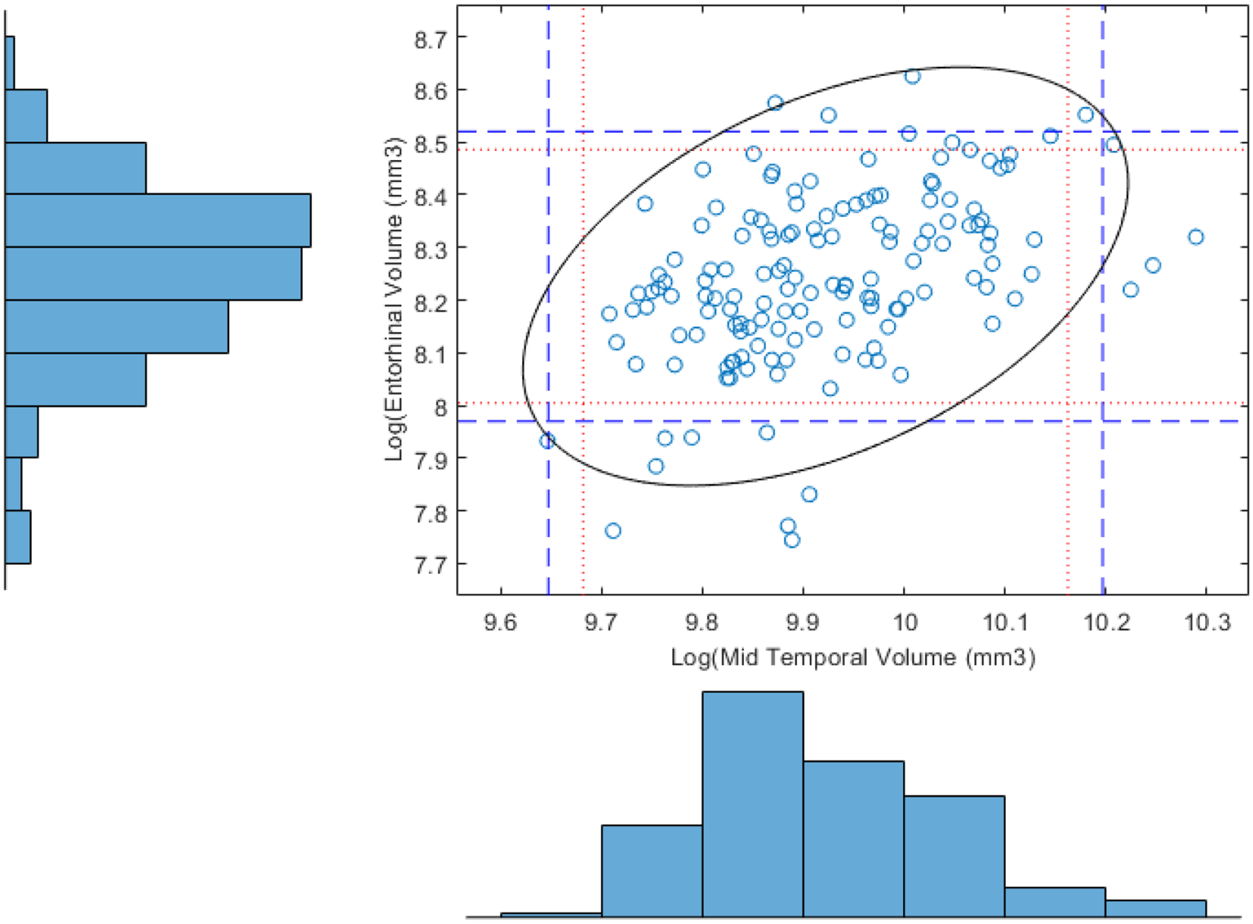
Multivariate distribution of two QIBs, Middle Temporal Volume and Entorhinal Cortex volume with multivariate (black ellipse) and univariate (red dotted lines) 95% confidence bounds. A second set of confidence bound (blue dashed lines) show a Bonferroni-corrected set of univariate confidence bounds.

Figure 2.

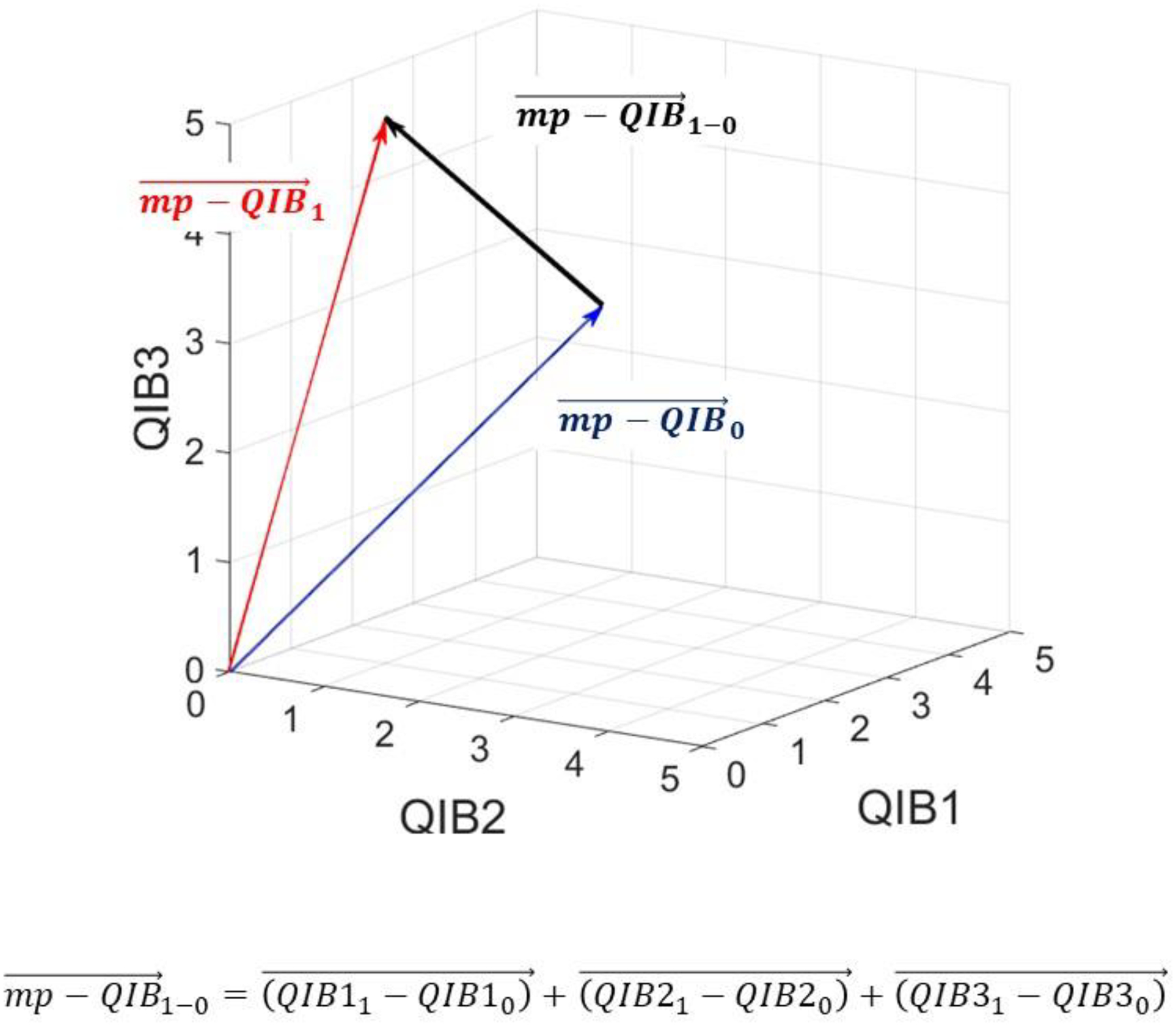
Vector depiction of the multivariate change in QIB orthogonal vectors over two time points and the difference vector

We present a method to mathematically combine two or more QIBs in a manner that does not degrade the performance of any single QIB while considering the complementary information from all QIBs that measure different, medically meaningful constructs of the disease. These constructs are disease characteristics that are not measured directly (otherwise known as latent) but are described by one or more QIBs. Examples of latent constructs of disease are metabolic activity measured by FDG-PET and cell death measured by volume or size. These constructs and the validity of the QIB to measure these constructs, otherwise referred to as construct validity, should be established with a validated QIB profile⁴³ before the development of the mp-QIB.

A well-defined and statistically rigorous multivariate function can combine the QIBs into a single mp-QIB that meets the definition of a QIB provided by Kessler et al.¹, which has the same metrological properties as a univariate QIB as outlined in Raunig et al.³.

2.1. Limitations of Current Multiple Biomarkers Solutions

Currently, the solutions to multiple quantitative measurements of disease most commonly use multiple endpoints (e.g., co-primary endpoints) or composites that use logic operators (i.e., AND and OR) to determine an event based on thresholds. These methods are described briefly and contrasted with the mp-QIB.

2.1.1. Multiple Co-Primary Endpoints

When using multiple co-primary endpoints univariately to evaluate treatment effects in a clinical trial, a common success criterion is that they all must be statistically significant to declare treatment efficacy^{39, 44–47}. The statistical implications are that for all of the co-primary endpoints, the treatment is expected to have an effect in the same direction, although each may evaluate a different disease construct at the same or different stages of disease progression. The directional hypotheses tested for the co-primary endpoints are

$$H_0:\left|{\Delta }_i\right|=0\mathit{\text{ for at least one of the }}I\mathit{\text{ biomakers}},$$

$$H_1:\left|{\Delta }_i\right|>0\mathit{\text{ for all of the }}I\mathit{\text{ biomakers}},$$

Where i = {1, 2, … I} indicates the i^th endpoint in the set of I endpoints, and Δ_i is the treatment versus placebo difference of the i^th endpoint. The null hypothesis H₀ can be rejected in favor of H₁ if each component null hypothesis H_0i: |Δ_i| = 0 is rejected in favor of H_1i: |Δ_i| > 0. However, unless the endpoints are highly correlated, this procedure can have very little power, known as the reverse multiplicity problem⁴³. To avoid lack of power, it is sometimes clinically acceptable to identify the most important of the co-primary endpoints as the single primary endpoint on which trial success is based, with all others considered as secondary and evaluated only if the primary endpoint is statistically significant based on a gatekeeping procedure^{47, 48}

The above hypotheses are contrasted to the classical hypothesis test of H₀: |Δ_i| = 0 for all I biomarkers vs. H₁: |Δ_i| ≥ 0 with strict inequality for at least one i. For this hypothesis test, O’Brien proposed a global test statistic (GTS) which, under H₀, is standard normal (mean 0, variance 1) when the endpoints are multivariate normal¹³. Pocock et al. extended O’Brien’s GTS to binary and survival data⁴⁹.

2.1.2. Composite Endpoints and Their Limitations

Cordoba defines a composite endpoint as “… two or more component outcomes” and “patients who have experienced any one of the events specified by the components are considered to have experienced the composite outcome.”⁵⁰. A composite endpoint can be attractive clinically since each endpoint describes the disease burden within each subject. Typically, composite endpoint decision rules are designed from the medical perspective and determine a binary outcome or event from a priori-defined thresholds applied to continuous QIBs and any hierarchical relationships. Continuous composite endpoints are also increasingly used as clinical trial endpoints^51–53. Examples of composite endpoints that use thresholds to define events are shown in Table 1.

Table 1.

Imaging techniques where use multiple QIBs are used as a composite to assess longitudinal change or response of a disease to treatment. The biomarkers are combined using rule-based combinations or as descriptor variables in a model of risk and are not considered as a multi-dimensional descriptor of disease change over time.

Reference	QIBs / Modality	Disease	Response	Comments
Choi13	CT Tumor size & Tumor density	Gastrointestinal stromal tumors (GIST)	Progression : size increase > 10% & change in density > - 15% Partial response	Rule based decision with multiple throesholds for response
Cheson14	PET CT	Lymphoma	CT: RECIST PET: 5-Point Scale	Rule based response without fully combining CT and PET
PI-RADS15	MRI PET Ultrasound	Prostate Cancer	T2, DWI, DCE, H-MRSI (PI-RADS) PET and ultrasound (aspirational)
Selmeryd16	Echocardiograph	Cardiac health	Multiple region velocities Mitral valve, early inflow, late inflow, mitral annular diastolic tissue velocity	Multiple endpoint determination of response
PI-RADS V 2.117,18	Multiparametric MRI (mpMRI)	Prostate Cancer	T2 and DCE Volume and Apparent Diffusion Coefficient	Multiple univariate MRI endpoints Volumes from multiple image types (T2, DCE-subtraction and ADC volume)
Eskildsen19	MRI	Alzheimer’s disease discrimination between MCI converters	Hippocampal grading Cortical Thickness of precuneus, superior temporal sulcas, parahippocampal gyrus	Linear Discriminant Classifier
Dennis20	MRI	NASH cTAG (cT1-AST-Glucose	Composite biomarker for detection compared to NAS Ordinal scores (ballooning, etc.)	Not a true composite. Biomarkers included as explanatory variables in a logistic regression model to derive a risk score.

The most common criticisms of composite endpoints are an implied assumption of uniform directionality of the components and component weights that are not clearly defined and often ad hoc⁵⁴. Another common critique of composite endpoints is that they obscure the relative clinical importance of the component endpoints. Hierarchical composites of prioritized endpoints have been proposed to emphasize composite components that may be medically more meaningful^55–62. However, these methods may not be appropriate when there are imbalances between treatment arms, the interpretation of the results is not completely clear, or the null hypothesis tests for non-inferiority rather than superiority^{63, 64}.

2.1.3. Multivariate techniques

Several multivariate methods exist that simultaneously provide a multivariate analysis of disease. Each method listed in Table 2 uses multiple endpoints to arrive at a simultaneous inference of the effects of the covariate(s). In Section 7.2 we will address the last listed test, the use of a single, vector-based metric derived by a pre-defined distance function that considers the correlation between endpoints in the derivation. A full description of the use of p-multiple vectors in statistical inference is beyond the scope of this paper and is detailed in Johnson and Wichern⁶⁵.

Table 2.

Multivariate methods for simultaneous inferential determination of longitudinal change

Test	Description	Advantages	Disadvantages
O’Brien’s OLS33	Ordinary Least Squares test for m=2 multiple endpoints	Simultaneous inference; controls false positive rate	More difficult to interpret than univariate; Requires knowledge of different test statistic Requires homoscedasticity
O’Brien’s GLS33	Generalized Least Squares test for m>2 multiple endpoints	Simultaneous inference; controls false positive rate; Correlated response variables accounted for	Difficult to interpret Loss of degrees of freedom; May still need to run univariate model
Joint Mixed Models34	Mixed models joint modeling using maximum likelihood estimation or related techniques	Includes variable correlation; Can use standard SAS or R procedures; Less computational problems for high dimensional data; Linear and non-linear models	Calculation of standard errors requires careful data manipulation
Traditional MANOVA / MANOVA-RM35	Test of m>=2 independent variables that are normally distributed	Allows for heteroscedasticity; Equivalent inference as Mahalanobis Distance for differences	Sensitive to collinearity and scaling; No single, intuitive measure of the disease outside of the test F-statistic or linearly averaged differences
Multiple Co-primary endpoints5,36	Test of m>=2 endpoints	Control of Type I error is well-studied and common; Medically determined endpoints;	No explicit consideration of endpoint correlation (typically); Reverse multiplicity and control of Type 2 error; Requires either that all endpoints are interchangeable or that there is a well-defined and prespecified hierarchy;
Hierachical composites of prioritized endpoints25–28	Within subject hierarchical assessment of endpoints in order of their priority	Non-parametric hypothesis test; Relatively powerful, especially in lieu of showing superiority in some endpoints and non-inferiority (NI) in others, because in general showing NI requires a large sample size.	Composite less interpretable clinically than individual endpoints; counter-examples exist in which a difference between groups in a hierarchical composite is driven by lower priority endpoints32
Mahalanobis Distance (Euclidean Distance)37	Test of m>=2 variables between 2 groups/treatments	Multivariate test of significance between treatments; Well established; Intuitive as an overall disease distance from 0, i.e., no disease; Simultaneous multivariate inference of all QIBs	Requires normal distribution with common covariance matrix; Can be sensitive to near-collinearity and QIB scaling

3.0. QIB COMPONENT PROPERTIES

Each QIB should be validated univariately as a reliable measure of its associated disease construct. Selection of each component QIB should consider the following:

• Medical importance, including disease construct being measured,

• Image acquisition,

• QIB measurement,

• QIB normality assumptions, and

• QIB technical performance characteristics (bias, precision, linearity, limit of quantitation, potential for cross-reaction, etc¹).

3.1. Medical importance

An initial pool of QIBs widely considered medically important in measuring disease progression should be compiled. These QIBs may include one or more data-derived radiomic QIBs addressed in Use Case 4¹¹. Examples of radiomics markers that may be associated with disease severity are surface texture, or “spicularity,” for solid tumors⁶⁶, and gray-level variance of the left hippocampus and gray-level cooccurrence matrix correlation of the right precuneus for Alzheimer’s Disease⁶⁷.

3.2. Image acquisition

Importantly, QIB candidate selection should also consider scanner availability, scanner settings, standard operating procedures, subject preparation, subject positioning, scanner settings, and other conditions for image acquisition. The ease of image acquisition needed to extract a complete set of component QIBs impacts the ability to limit missing QIBs. Methods to impute one or more missing QIBs are discussed later in Section 3.4. Still, imputed data, even when using the widely recommended method of multiple imputation, are uncertain and thus do not completely reduce the impact of missing data, especially at the patient level⁶⁸.

3.3. QIB Measurements

A QIB measurement is a quantitative variable with a meaningful zero (i.e., a ratio variable) or one that can be used to measure change (i.e., an interval variable). Each QIB may be continuous or discretized but cannot be ordinal. For example, researchers may wish to group QIB measurements into categories defined by empirical quantiles, e.g., quartiles. However, the categorical scores of a Likert scale (e.g., 0-None /1-Mild /2-Moderate /3-Severe) are ordinal and thus do not meet the definition of a QIB.

Very often, rounded or truncated data often occur when the image data output is taken from a user display system where the displayed value is primarily for clinical use. When possible, it is best to use unrounded or untruncated data when available to avoid bias or inaccurate variance estimations⁶⁹

For the development of the mp-QIB, the set of QIBs must be multivariate normal, in which case each QIB component must be normally distributed or transformable to a normal distribution. Normality transforms may be defined canonically (e.g., log transform) or by using a power transform method⁷⁰.

3.4. Missing Data and Data Below the Limit of Quantification

It’s possible and even likely that there will be missing QIB data among the multiple QIB components of the mp-QIB. A QIB component may be missing for several reasons, including a missing or unacceptably poor quality scan, a calculated value beyond what is physically possible, scanner availability, or measurements outside the QIB profiled measurement interval. Most often, this last reason is due to a QIB value below the lower limit of quantification (BLOQ)⁷¹, which the scanner manufacturer usually defines as a quality control measure.

For novel or specialized imaging modalities, widespread unavailability for the context of use may preclude the use of that QIB for the mp-QIB model development. Missing QIB values due to a more random occurrence can be addressed by either casewise deletion of the multivariate observation or imputation of the missing values⁷². In general, casewise deletion is discouraged unless missing values are rare or the unlikely assumption holds that the data are missing completely at random (MCAR), that is, the probability of missing data does not depend on any data^{73, 74}. Any mp-QIB profile should address missing data with a sensitivity analysis of different missing data scenarios.

Data are missing at random (MAR) when the probability of missing values depends on the observed data. When data are MAR, casewise deletion introduces bias into the statistical analysis. Under MAR, multiple imputation, among other imputation techniques, is a quickly implemented alternative to casewise deletion that accounts for missing data and their uncertainty. An abbreviated list of the imputation methods and their advantages and disadvantages are shown in Table 3. Deep learning imputation models⁷⁵, not shown in Table 3, are promising but are not commonly used and are not discussed further.

Table 3.

Multivariate imputation methods and their advantages and disadvantages for Use Case 1, the multivariate descriptor of health.

Method	Description	Advantages	Disadvantages
Multivariate Imputation by Chained Equations (MICE)43	A multiple imputation method using a set of iterative regression models.	Continuous data handling Regressors can also be incomplete Widely used and accepted	Longitudinal data can be a problem Specification of conditional models which may be difficult to know a priori
Nearest Neighbor (NN) estimation	A supervised pattern recognition method based on the distance to each pair of observations based on non-missing variables and imputing based on a weighted mean	Continuous data handling May outperform MICE when transformed data are slightly skewed Consistent with Euclidean distance mp-QIB function Requires only one non-missing value Several modifications and versions to accommodate missingness patterns	Requires specification of a tuning parameter that can have a large effect on the results
Random Forest (RF)44	A sequential, machine learning imputation process that predicts missing data from a training set consisting of observed data	Robust / Non-parametric Good performance in high dimensional QIBs Handles non-linear relationships	Training on observed data Can be severely biased44
Multivariate Normal Imputation (MVNI)45,46	An iterative process that imputes missing data from multivariate normal distribution parameters using an expectation-maximization algorithm.	Performance equal to MICE when data are multivariate normal and no missing patterns Assumption of multivariate normal is given for this Use Case Robust to distribution misspecification	Performance may be degraded for misspecification of multivariate normal data
Selection Model:	Joint distribution of data Y and missingness indicator M is partititioned into f(M,Y|θ, ψ) = f(Y|θ)f(M|Y, ψ).	Under MAR, inference can be based on the likelihood ignoring the missing data mechanism, that is, on f(Yobs|θ) where Yobs are the observed data.	May not be clinically as easily understood as a pattern mixture model because distribution of data not stratified by whether it is missing or not.
Pattern Mixture Model:.	Joint distribution of data Y and missingness indicator M is partititioned into f(M,Y|ξ,ω) = f(Y|M,ξ)f(M|ω)	PMM can be useful for modeling the distribution of data missing not at random (MNAR).	Not as well understood as selection models.
Bayesian inference:	Likelihood given observed data is augmented with draws of missing data from their full conditional posterior predictive distribution given observed data and a sample of the parameter values from their full conditional distribution	Data augmentation simplifies the likelihood and thus the Gibbs sampler or other Monte Carlo Markov Chain algorithm for computing the joint posterior distribution.	Unfamiliarity of Bayesian inference; modeling is required, in particular specification of the prior distribution.
Bootstrap imputation47–49	Methods for bootstrapping after multiple imputation or imputation following bootstrap.	Principled, non-parametric approach for incorporating missing observation uncertainty into analysis.	Implementation varies

Some multivariate methods for multiple imputation rely on multivariate normality; therefore, imputation for calculating the mp-QIB should be conducted using the normal transformed QIBs when appropriate. Importantly, imputations for missing QIBs should be checked for reasonableness at the subject and cohort levels.

When QIB values are below the manufacturer-specified quality control (QC) lower limit, the value recorded by the scanner is “BLOQ” or “<LOQ” or simply as missing. Some examples are lower limits of iodine and iron content for dual-energy computed tomography (DECT)⁷⁶ and the wall filter settings for Doppler ultrasound frequencies^{77, 78}. Consequently, calculating the mp-QIB must consider the existence of BLOQ values. Therefore, when BLOQs occur often, some consideration should be given to removing that QIB from the choice of QIB components, at least for the intended subject population..

These values are very often actually measured by the scanner and only output as “BLOQ” or “<LOQ.” It is recommended that the actual measured values be used if it is possible to recover these from the scanner output.^{79, 80}. If they cannot be recovered, the BLOQ values can be imputed using multiple imputation or Bayesian methods^81–85. Often, LOQ/2 is used to impute BLOQ values for ease of implementation. However, Harel et al. and others have demonstrated that this method can result in a significant bias for even modest incidences of BLOQ values^{81, 85–87}. In addition to imputation schemes, maximum likelihood models assuming a truncated normal distribution are also good at reducing bias in mean and variance estimation⁸⁷.

It is recommended that if single imputation by LOQ/2 is used for convenience, as a first step in developing an mp-QIB, additional analyses should be conducted using the methods included in Table 3 to verify or confirm the results.

3.5. QIB Technical Performance

The technical performance of the mp-QIB will follow that of a single QIB with differences due to the multivariate distribution of the component QIBs, the requirement of the covariance of the QIBs to be positive definite, and the robustness of the mp-QIB to missing QIB components. Additionally, newly finalized FDA guidance for industry and FDA staff on quantitative imaging in radiological devices offers guidance for metrological performance metrics⁸⁸.

The technical performance of each component QIB should be profiled before the selection of the QIB from the pool of QIB candidates. Each component QIB should meet the following conditions:

• Normally distributed or transformable to a normal distribution

• Linear relationship to the measurand (linearity)

• Linear measurement interval; and

• Longitudinal change is observed or known for the intended disease.

The linear relationship to the measurand is critical to demonstrate mp-QIB linearity in the absence of a multiparametric measurand. The linearity of each QIB to its respective measurand should have a slope of 1 to avoid the interpretability of non-constant bias. A non-zero intercept for the individual QIB will be canceled when mean-centering or evaluating differences occur. See Supplemental Material 1 for proof of the use of QIB linearity to define mp-QIB linearity.

4.0. THE MP-QIB MODEL

4.1. Concept

For QIBs that describe a set of n constructs of overall health, Ψ, the set of QIBs, can be represented as

$$\Psi =\left\{{\psi }_{11},{\psi }_{12},\dots ,{\psi }_{1k(1)},\dots {\psi }_{n1},{\psi }_{n2},\dots {\psi }_{nk(n),}\right\}$$

where there are k(n) variables per construct and k>0 for all n constructs (see Figure 3). In this example, different imaging modalities provide quantitative biomarkers for different constructs of chronic liver disease⁸⁹.

Figure 3.

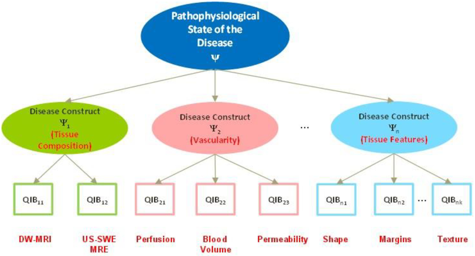
Depiction of the variables that describe the different constructs that define the total disease pathophysiology (ψ). The imaging examples shown provide biomarkers of liver disease

In contrast to a multiparametric risk model⁸, the mp-QIB descriptor described here provides a measure of the state of the disease rather than acting as a predictor of risk or phenotype. The multivariate variable for the ith subject with p QIBs is

$$X_i=\left(X_{i,1},\dots ,X_{i,p}\right).$$ Equation 1

Harrell recommends the number of subjects during the model development phase of the mp-QIB to be n≥15p, which is feasible in most cases due to the limited number of available QIBs⁹⁰.

As shown in Figure 3, the latent state of the patient, Ψ, is measured as a function of the set of the multivariate QIBs

$$\Psi (X)=g(X)+v$$ Equation 2

where g mathematically combines the n × p array of QIBs and v is measurement error. For clarity, in the sections to follow,

$$\text{mp-QIB}\stackrel{\text{def}}{=}\Psi (X)$$ Equation 3

In its simplest form, g is defined as the vector sum of X for a set of orthonormal vectors, X, with magnitude ‖X‖ and direction Φ where

$$\Vert X_i\Vert =\sqrt{{\text{X}}_{\text{i},1}^2+\dots +{\text{X}}_{\text{i},\text{p}}^2}$$ Equation 4

$$\Phi =\text{arccosine}\left\{\frac{X_1}{\parallel X\parallel },\dots ,\frac{X_p}{\parallel X\parallel }\right\}$$ Equation 5

In reality, the vector components of X are likely and even expected to be at least moderately correlated. A Euclidean distance function must also consider the degrees of similarity (i.e., correlations) between the multivariate set of vectors. This similarity takes the form of the correlation matrix, which can be easily shown to be equal to cosine similarity, defined as

$$cos(\alpha )=\frac{X_i\cdot X_j}{\Vert X_i\Vert \Vert X_j\Vert },$$ Equation 6

often used in multivariate neural networks for similar feature selection^{91, 92}.

The mathematical function, g, maps each multivariate vector, X_i, to a unique mp-QIB_i. However, a unique mapping is not guaranteed for all distance functions. For example, Kullback-Leibler divergence often used in AI models is intrinsically asymmetric, does not have a unique mapping, and does not satisfy triangle inequality⁹³. Details of the function g(X) are described in Section 4.2.

4.2. The mp-QIB model function

For the simplest example of two independent and uncorrelated QIBs, each is distributed marginally as standard normal or symbolically as ~N(0,1). The Euclidean distance of a multivariate vector from a multivariate reference vector defines the function, g as

$$g\left(X_i\right)=\sqrt{{\left(X_{i,1}-X_{i,\text{r}1}\right)}^2+{\left(X_{i,2}-X_{i,\text{r}2}\right)}^2}$$ Equation 7

Where X_i,j is the j^th QIB of the i^th subject, and X_irj is the j^th QIB reference vector

The covariance-normalized Euclidean distance between two multivariate vectors is referred to as the Mahalanobis Distance (DM)⁹⁴. Alternately, the squared Mahalanobis Distance (DM2) is commonly used in multivariate pattern recognition and clustering⁹⁵.

DM2 can be used to describe the disease states of subjects sampled from a population. For example, QIBs X, Y, and Z can be used to characterize subjects as cognitively normal (CN), having mild cognitive impairment (MCI), or having Alzheimer’s Disease (AD). For DM2, the reference vector is the zero vector $\overrightarrow{0}$. DM2 is understood to be the squared distance from 0 and is defined as

$$\text{DM}2={\text{X}}^{\text{T}}{\Sigma }^{-1}\text{X},$$ Equation 8

where,

$$\Sigma =E\left[[\text{X}-\text{E}[X]]{[X-\text{E}[\text{X}]]}^{\text{T}}\right]$$ Equation 9

is the population covariance matrix of the QIBs, and E[X] = (μ₁, μ₂, …, μ_p) is the array of QIB population means. Since the population variance is not typically known, the sample covariance matrix, S, is used instead and defined as,

$$S=\frac{1}{n-1}{\sum }_{i=1}^n\left(X_i-\overline{X}\right){\left(X_i-\overline{X}\right)}^T,$$ Equation 10

where $\overline{X}=\frac{1}{n}{\sum }_{i=1}^n{X}_i=\left({\overline{X}}_1,{\overline{X}}_2,\dots ,{\overline{X}}_p\right)$ is the array of QIB sample means. Therefore, the DM2 statistic will be hereafter defined as DM2 = X^TS⁻¹X. Since DM2 is only defined for a multivariate normal set of QIBs, (n − p)DM2/p(n − 1) follows a non-central F distribution. In large sample sizes, this distribution can be closely approximated as non-central ${\chi }_{\text{df}=\text{p}}^2$ with non-centrality parameter ${\lambda }^2={\sum }_{i=1}^p{\mu }_i^2$⁹⁶. Sufficient numbers for large sample sizes depend on both p and n and will be discussed further in Section 7.4.

To reduce the need to consider the non-centrality parameter in the development of the mp-QIB model, X is centralized as

$$\text{X}\leftarrow \text{X}-E[\text{X}]$$ Equation 11

to simplify the calculation of the sample means and variances⁹⁷ (see Section 8.3.1). The difference between two subject-paired mp-QIB endpoints is defined as the DM2 of the differences between vectors (i.e., ‖X₂ − X₁‖) and not as DM₂ − DM₁ since two identical values for DM can be defined by two entirely different sets of QIB vectors. Thus

$$D{M}_{2-1}=\sqrt{{\left(X_2-X_1\right)}^T{\mathit{S}}_{2-1}{}^{-1}\left({\text{X}}_2-{\text{X}}_1\right)},$$ Equation 12

where

$$S=\frac{1}{n-1}{\sum }_{i=1}^n\left(X_2-X_1\right){\left(X_2-X_1\right)}^T,$$ Equation 13

If change over time is the interest, for example, treatment effects, Equation 11 is modified slightly to measure the average vector distance between two populations as follows:

$$DM{(\mathit{\text{trt effect }})}_{2-1}=\sqrt{\frac{n_{trt}{n}_{pbo}}{n_{trt}+n_{pbo}}{(DX)}^T{S_{\text{pooled }}}^{-1}(DX)}$$ Equation 14

where

$$S_{\mathit{\text{pooled}}}=\frac{\left(n_{trt}-1\right)S_{2-1,trt}+\left(n_{pbo}-1\right)S_{2-1,pbo}}{n_{trt}+n_{pbo}-2}.$$ Equation 15

and

$$DX=\left(\left(\overline{X{(\text{t}=\text{T})}_{\text{trt}}}-\overline{X{(\text{t}=0)}_{\text{trt}}}\right)-\left(\overline{X{(\text{t}=\text{T})}_{\text{pbo}}}-\overline{X{(\text{t}=0)}_{\text{pbo}}}\right)\right)$$ Equation 16

5.0. CHOOSING THE QIB COMPONENTS OF THE MP-QIB

The initial candidate pool of QIBs should be chosen based on medical relevance and intended use. Once the candidate pool is selected, it should then be reduced to a more parsimonious set based on medical, imaging, and technical performance. Reasons to exclude a QIB include but are not limited to scanner availability, inability to transform to normality, poor reliability for measuring change, missingness, difficult or uncommon image acquisition, and frequent outliers.

Many commonly used methods for multiple feature reduction treat the QIBs as multiple variables used to explain or predict a dependent variable. Here, the dependent or descriptor variable is the mp-QIB; therefore, multivariate methods such as principle components better serve the development of the mp-QIB. The steps shown in the following section describe the selection of QIBs when the true state of the disease is unknown or unavailable.

5.1. Steps for Multiple QIB Selection

5.1.1. Step 1: Build an mp-QIB candidate pool.

• Build a candidate QIB pool based on expert opinions without necessarily relying on a consensus opinion

• Example: Tumor progression⁹⁸

  • Tumor burden: Objective measure of size (CT/MRI)
  • Tumor viability: Temporal perfusion (MRI)
  • Tumor metabolism: FDG-PET
  • Dynamic susceptibility: DCE-MRI and DSC
  • Diffusion characteristics: MRI-DTI

5.1.2. Step 2: Review the QIB pool by all experts:

The Delphi or a Delphi-like method can help arrive at a medical consensus for a reduced QIB candidate pool^99–101.

5.1.3. Step 3: Evaluate QIB pool variables for selection and dimension reduction:

Once the medically relevant candidate QIBs are collected, this pool can be further reduced based on the mathematical and practical concerns that include the following.

• QIB profile: The QIBs should have use profiles that reliably measure changes in the intended subject population.

• QIB distribution properties: Each candidate QIB should be a ratio variable with a meaningful zero or interval variable when only the difference vector is used.

• QIB measurement interval: The dynamic range or measurement interval should be sufficient for the intended use.

• Medical confidence: Changes in the QIB correspond to a change in the disease severity, and conversely, changes in the disease are reflected in changes in the QIB.

• Image acquisition: Calibrated scanners and imaging availability reduce the need for missing data imputation.

• Image Quantitation: Quantitation algorithms should be validated and equivalent⁵.

• Missingness: Missing QIB components should be MAR or MCAR.

Each QIB should measure a construct or specific disease feature (see Figure 3). The following are high-level functional considerations for QIB selection from the initial candidate QIB pool:

• Highly correlated QIBs: Highly correlated QIBs indicate that they essentially measure the same thing and may result in problems when inverting the covariance, S (see Equation 10). As a general rule, correlations between two QIBs that exceed 0.8 should choose one QIB over the other

• Disease construct measurement: Each disease construct should be measured by at least one QIB and, ideally, more than three QIBs. The maximum number of QIBs per construct greatly depends on the complexity of a particular construct. Therefore, the limitation of QIBs is a more practical concern.

• Cross-construct QIBs: As a general rule, a QIB that covers multiple disease constructs should be avoided, though there will be exceptions when the constructs describe a higher-level latent construct.

• Repeatable: Each candidate QIB should demonstrate the ability to obtain the same measurement under identical (or near identical) conditions. The repeatability variance should be small enough to determine a clinically meaningful minimum detectable difference.

• Reproducible: Each candidate QIB should demonstrate the ability to obtain the same measurement under different imaging conditions, such as different scanners, sites, or readers.

• Ability to measure change: Each candidate QIB should be expected to change with changes in the disease severity.

5.1.4. Step 4: Exploratory Factor Analysis (EFA) and dimension reduction:

This step is primarily meant to reduce the set of QIBs to those that measure the originally-intended disease constructs. The multiple QIBs are not used to predict or describe a clinical outcome; instead, they are evaluated in this step as latent construct descriptors. Each QIB loads primarily to only one construct or factor. Highly correlated QIBs that describe the same construct should be reviewed for possibly excluding one of them^{65, 102–104}.

The result of an EFA should determine

• Whether the factors match the a priori determination of the constructs;

• That the QIBs are primarily associated with only one factor;

• That the factors and associated QIBs minimize the correlation between latent constructs; and

• That the interpretation of the factors is medically consistent.

A complete set of steps and instructions for using SAS/PROC FACTOR is provided by O’Rourke and Hatcher¹⁰⁴, which can also be used to guide the user in R/factanal.

5.1.5. Step 5: Confirmatory Factor Analysis (CFA)

A confirmatory factor analysis (CFA) uses the estimated structure from EFA to test the hypothesis that the relationship between QIBs and the factors or constructs exists. CFA differs from EFA since the variables and number of factors are known¹⁰⁵93. Confirmatory factor analysis will be discussed in more detail in the next section as a method for model validation.

6.0. MODEL EVALUATION

Evaluation for the mp-QIB model will primarily demonstrate the mp-QIB model’s superiority to any univariate QIBs to lower or minimum detectable effect size. Cross-validation helps to ensure against overfitting when finalizing the component QIBs. Typically, model cross-validation is conducted using a known clinical outcome or state as the dependent variable, such as survival in a risk model or a known phenotype in a classification model^{8, 9}. Profiling the mp-QIB will have no comparable clinical reference to evaluate performance. In addition, multiple QIB change scenarios and QIB covariance can make the option of a multivariate phantom unlikely. Therefore, mp-QIB validation should be conducted in three phases:

1. Internal cross-validation of the constructs/factors and QIBs for each factor;

2. Internal confirmation of the QIB component selection using CFA; and

3. External validation of the superior ability of the mp-QIB to detect change.

6.1. QIB Selection Cross-Validation

Cross-validation of the QIB selection results from the EFA should be conducted to help ensure that the results can be generalized for the intended use. For example, a k-fold cross-validation method is best when datasets are moderate to small and hold-out datasets can be considered when the dataset is large. Additionally, bootstrap methods for factor identification and QIB selection allow for ensemble-averaging for loading factor determination.

6.2. mp-QIB Model QIB Component Confirmation

The CFA acts to confirm and test that the QIBs load onto the now-defined constructs, that the model meets parsimony requirements based on the covariance structure of the QIBs, and that the QIBs actually measure the constructs of interest. The CFA analysis solves the linear equation

$$y=\Lambda \eta +\epsilon$$

where y is a vector of observed indicators, Λ is the common standardized loading factor matrix, η is a vector of latent factor scores that are normally distributed and uncorrelated, and ε is a vector of unique QIB errors. CFA allows the latent factors to covary, whereas the EFA assumes that the latent factors were not correlated.

A general rule for conducting CFA is at least three variables per factor. However, in reality, the number of QIBs will be limited by technology, cost, and patient burden, and it may not be possible to meet this criterion. Therefore, while the overall results may be consistent with EFA, the fit statistics in these cases should consider this limitation and any impact of small sample sizes on the asymptotic test statistics^{106, 107}.

CFA is traditionally used for multivariate psychometric instrument development when multiple manifest variables, such as scale items, are used to provide measures of a specific latent disease construct. Similarly, the mp-QIB component QIBs are measured quantitative variables determined by the latent disease constructs. Since the CFA assumptions include multivariate normality of the variables and covariance between the factors, CFA may also prove helpful in developing the mp-QIB. Confirmatory factor analysis may be conducted using either PROC CALIS with SAS® or with R using the “lavaan.r” package. The procedures for the conduct of CFA are provided in detail by O’Rourke and Hatcher¹⁰⁴ and will not be detailed further.

6.2.1. Known Groups Analysis

The use of groups in which the disease is known to affect a specific disease construct may be used to validate the mp-QIB by detecting known or predictable changes. Examples may include a known genetic mutation or known changes due to age. Modeling disease progression may be best measured by multiple QIBs that could be followed through the different states of the disease by the progressive inclusion of different constructs. Conversely, a therapeutic response may be defined by the resolution of the progression in reverse. Importantly, a known-groups analysis must not define the groups using any component QIBs.

7.0. STUDY DESIGN

7.1. Study Design

The study designs for mp-QIB development will be similar to those provided in Raunig et al.³. They should follow the same considerations for longitudinal data and repeatability/reproducibility estimates precision. Due to the increased likelihood of missing data from multiple imaging modalities, study designs should also consider sample sizes under the expectation of increased missingness.

7.2. Tests of Hypotheses

The goal of the mp-QIB is to be more sensitive to changes in the disease than any single QIB. Achieving this goal can best be demonstrated by requiring that any test for superiority compare standardized differences, such as that between two longitudinal visits, shown below as Cohen’s d

$$d=\frac{\left|X-X_1\right|}{\sigma }$$ Equation 17

where σ is the population standard deviation of the error. More commonly, the sample standard deviation is used instead (Hedge’s g) as

$$g=\sqrt{2}\frac{\left|\overline{X_2-X_1}\right|}{s_{2-1}}$$ Equation 18

where s₂₋₁ is the standard deviation of the difference of the repeated measurements X₁ and X₂ under no-change conditions. If explanatory covariates are used, the repeated measures within-subject variance can be determined as a maximum-likelihood estimate from a mixed model with repeated measures.

When used for measuring longitudinal change, the mp-QIB may test the null hypothesis that the mp-QIB is not better than any component QIB, stated as the following null and alternative hypotheses

$$H_0:{\delta }_{mp-QIB}\le {\delta }_{QI{B}_i},\mathit{\text{ for any }}i=1,\dots ,p$$

$$H_A:{\delta }_{mp-QIB}>{\delta }_{QI{B}_i},\mathit{\text{ for all }}i=1,\dots ,p$$

where δ is the mean effect size. The challenge of demonstrating the superiority of the mp-QIB is known as “reverse multiplicity,” or that the mp-QIB must be better than all QIBs to reject the null hypothesis.

In terms of sub-hypotheses for each QIB,

$$H_0:\bigcup _{i=1}^p{H}_{0i},H_{0i}:{\delta }_{mp-QIB}\le {\delta }_{QI{B}_i}$$

$$H_A:\bigcap _{i=1}^p{H}_{Ai},H_{Ai}:{\delta }_{mp-QIB}>{\delta }_{QI{B}_i}$$

The intersection-union test (IUT) of H₀ is carried out by testing each H_0i at the nominal significance level (e.g., 2.5%). If all are rejected, then H₀ is rejected. Though there is no inflation of the Type 1 error rate under the IUT, the procedure is conservative, resulting in low power (inflated Type II error)⁴⁴.

Since each candidate QIB should be fully profiled, a hierarchically clinical or medical level of importance may provide an alternative set of hypotheses to demonstrate that the mp-QIB is more sensitive than the clinically most important QIB.

If the QIBs are ranked in a predetermined order of importance such that d₁ > d₂ > … > d_p, then the null and alternative hypotheses used to demonstrate mp-QIB superiority become the following:

$$H_0:d_{mp-QIB}\le d_1,\text{ and }$$

$$H_A:d_{mp-QIB}>d_{QI{B}_i},\mathit{\text{ for all }}i=1,\dots ,p.$$

In fixed sequence multiple endpoint hypothesis tests, such as that described above, the fallback method provides an opportunity to test endpoints later to de-risk misspecification of the QIB order when there is no clear number one^{108, 109}.

Because ${\widehat{d}}_{mp-QIB}$ and ${\widehat{d}}_{QI{B}_i}$ are correlated and likely and non-normal, tests of H_0i may need to use non-parametric paired tests such as the Wilcoxon Sign Test¹¹⁰.

7.3. Retrospective versus Prospective Data

Data to develop, test, and validate an mp-QIB biomarker can be acquired in a prospectively designed study or, often more likely, using previously acquired epidemiological natural history data. The advantages of retrospective data include cost, time, and number and breadth of subjects, while the major disadvantage is the lack of control over the subject population. The Alzheimer’s Disease Neuroimaging Initiative (ADNI) is a well-known example of a source of multiple neuroimaging modalities¹¹¹. A list of the advantages and disadvantages of each type of study is shown in Table 4.

Table 4.

Advantages and disadvantages of the use of retrospective and prospective data in mp QIB development.

Type of Study	Advantages	Disadvantages
Retrospective	Large databases that include patients over a broad range of disease severity and patient demographics Existence of healthy normal controls in a known-groups proof-of-concept analysis Data collection already done Ability to use other analyses to inform on the desired objectives Can sometimes use patient data to match the desired intended use patient profile Cost may be less than the cost of a prospectively designed study. May be only method of acquiring sufficient data on rare disease populations	Databases may be private with restricted access and restrictions on use Subjects are not typically randomized and control of biases not guaranteed or may not even be possible Healthy controls not always available requiring a prospective collection that would match the database Influenced by other analyses Patient population may not be equivalent for the intended use of the mp-QIB May not be able to conduct an external cross-validation requiring prospectively acquired data with different patient population
Prospective	Can specify the subject population(s) Greater control of bias if the sample size is sufficiently large Greater trust in the results Piggyback on current therapeutic intervention study can provide data for known-groups validity on measuring disease progression versus known or standard of care intervention (SOC)	Does not require external organizational approval with restricted use. Expensive and requires all of the costs with study start-up and recruiting that can be Slow recruitment when there is no therapeutic benefit can stop a study
Combination Retrospective-then-Prospective85	Uses available data for mp-QIB development and prospectively acquired data for validation Retrospective data analysis can provide information on the optimal patient inclusion/exclusion criteria in the prospective study Prospective numbers and data costs minimized when used as validation compared to use as both development, testing and validation	Requires that both types of data be available

7.4. Sample Size

The samples should span the measurement range of each QIB. Also, the size should be large enough to provide sufficient degrees of freedom to estimate repeatability and reproducibility variances. Also, sample sizes should provide adequate power to detect superiority to the component QIBs for differences.

In addition to sample size for precision, the number of QIBs should also consider the following items.

• Exploratory Factor Analysis should ideally have more than 3 QIBs per construct¹⁰⁴ but may need to be relaxed due to limitations of available QIBs.

• Sample size estimates for EFA and CFA can be calculated based on the bounds of the root mean square error of approximation (RMSEA) of the resulting model¹¹². Typical values for factor analysis sample sizes are approximately 200, though smaller sample sizes may be adequate for typical numbers of QIBs. For comparison, multiple co-primary endpoints sample size determination methods described by Kolampally and Kohl¹¹³ and Yang et al.¹¹⁴, provide a general approach for multiple correlated endpoints (See Supplement 4).

• Sample sizes needed to treat the mean-centered DM2 as a central χ² distribution with p degrees of freedom depend on both p and n. Results shown by Rencher provide approximate asymptotic sample sizes for different p¹¹⁵. For a feasible p=5 QIBs, Rencher shows, with some caution, that a large sample size is n=100.

7.5. Inclusion / Exclusion criteria

The criteria for subject inclusion should identically reflect the claim and context of intended use as well as the impact of missing data.

8.0. TECHNICAL PERFORMANCE

The technical performance metrics of the mp-QIB closely follow those for univariate QIBs³ with differences due to the distribution properties.

8.1. Estimation of the multivariate sample variance, S

The QIB covariance matrix, S, must be positive definite to be inverted when calculating DM2. When including two or more QIBs that are highly correlated, inverting S may fail due to the inclusion of near-collinear QIBs. Highly unbalanced scaling of the variables can also result in an unstable inverse covariance matrix that cannot be directly inverted. Covariance matrices that cannot be directly inverted may be regularized using the Hubert method of singular value decomposition, which sets problematic eigenvalues to a small number and then reconstructs S¹¹⁶. More commonly, the generalized inverse or pseudo-inverse of square matrices are used to avoid singularity problems^{117, 118}.

Extensive data sets may require large amounts of computational time to calculate S. Methods to overcome long computation times include Cholesky (LU) decomposition and the minimum covariance determinant (MCD) method using the FAST-MCD algorithm of Rousseeuw and VanDriessen^{116, 119}. The FAST-MCD algorithm can be found in R (rrcov, robust and robustbase), S-PLUS (cov.mcd), and SAS (Proc RobustReg). The MCD algorithm is a robust estimator resistant to outliers that can significantly affect the variance and covariance estimations. Additionally, caution should be exercised when using LU decomposition due to limitations associated with numerical integration, and double formatted numbers are preferred to floating point number format.

8.2. Linearity/Bias Monotonicity of the model function g

The model function, g, must meet the requirement that for two vectors, X₁ and X₂, the distance to the sum of the vectors from the origin is less than or equal to the sum of the magnitudes of the vectors, known as the triangle inequality theorem. For two QIBs, defined as vectors from the origin (re the requirement to be a ratio variable),

$$\Vert X_{i,1}+X_{i,2}\Vert \le \Vert X_{i,1}\Vert +\Vert X_{i,2}\Vert$$ Equation 19

Satisfaction of triangle inequality will be the basis for establishing linearity to a virtual mp-QIB measurand.

Since there is no measurand for the mp-QIB to be compared against for linearity and bias, the functional requirements to meet the triangle inequality will be met when each of the QIBs has a linear relationship to its respective measurand (See Supplement 1). A non-zero intercept will be canceled for mean-centered DM or when difference vectors are used. When a single time point measures a disease status, a QIB constant bias will be included in the noncentrality parameter. Slopes not equal to 1 translate to a QIB-dependent non-constant noncentrality parameter.

8.3. Repeatability / Reproducibility

The following sections describe estimation for S under repeatable and reproducible conditions.

8.3.1. Repeatability

8.3.1.1. Univariate Repeatability Coefficient-RC

The univariate repeatability coefficient (RC) is the least significant difference, at the 5% significance level, between two repeated measurements of a QIB taken under identical conditions^{3, 5}.

$$RC=1.96\sqrt{2}{\sigma }_W=2.77{\sigma }_W$$ Equation 20

where σ_w is the within-subject standard deviation of the repeated QIB measurements. The formula for RC above is valid when the degrees of freedom, v, is large for estimating σ_w. However, when v is not large, σ_w is estimated as s_w with error and the more general formula

$$RC=\sqrt{2}{t}_{0.975}(v)s_W$$ Equation 21

applies, where t_q(v) is the qth quantile of a Student’s t distribution with v degrees of freedom.

RC is a special case of the total deviation index TDI_q, which is a quantile q in the distribution of absolute differences between a measurement and another measurement obtained by a different measurement procedure¹²⁰.

8.3.1.2. Multivariate Repeatability Coefficient-RC_mp

The multiparametric repeatability coefficient (RC_mp) can be defined analogously by considering the multivariate generalization of the t-statistic, the Hotelling T² statistic where

$$T^2=D{M}_{2-1}^2$$ Equation 22

and DM₂₋₁ is defined as in Equation 12. Under the null hypothesis that E(DX) = 0,

$$\frac{T^2}{v}\frac{v-p+1}{2p}~F(p,v-p+1),$$ Equation 23

where v is the degrees of freedom for estimating the covariance matrix as S and F(v₁, v₂) is the F distribution with v₁ and v₂ degrees of freedom. For example, in test-retest studies of n subjects with two repeated measures per subject, v = 2n − n = n. Therefore, at significance level α = 0.05, the multiparametric repeatability coefficient for DM₂₋₁ is

$$R{C}_{mp}\left(D{M}_{2-1}\right)=\sqrt{\frac{2pv}{v-p+1}{F}_{0.95}(p,v-p+1)}$$ Equation 24

If v is very large compared with p, then, approximately, T²~2χ²(p), where χ²(p) is the chi-square distribution with p degrees of freedom, and

$$R{C}_{mp}\left(D{M}_{2-1}\right)=\sqrt{2{\chi }_{0.95}^{\mathbf{2}}(p)}$$ Equation 25

The multiparametric limits of agreement (mp-LOA) are then defined as

$$LO{A}_{mp}(\mathit{\text{repeatability}})=\left(0,R{C}_{mp}\right).$$ Equation 26

which can be interpreted as the 95% prediction region for the true differences of DM_2–1 under identical image acquisition conditions.

A complete description of the derivation of RC_mp for any number of repeated measures per subject and any significance level is shown in Supplements 2 and 3.

The agreement between two repeated measures of mp-QIBs can be measured in the aggregate using the multivariate concordance correlation coefficient (MCCC), extending Lin’s CCC beyond the agreement of univariate QIBs.

$$\mathit{\text{MCCC}}=1-\frac{\sqrt{\mathit{\text{trace}}((I-M)(I-M))}}{\sqrt{\mathit{\text{trace}}(I)}}$$

Where I is the identity matrix and M is the multivariate ratio of variances¹²¹. Details for the calculation of MCCC are found in Supplement 5

When combining repeatability from different groups, e.g., different sites, if a common covariance is assumed, the pooled covariance will define S_w for repeatability as follows:

$$S_{w,p}={\sum }_{i=1}^k\left(v_i-1\right)S_{w,i}/{\sum }_{i=1}^k\left(v_i-1\right)$$ Equation 27

Test-retest repeatability may be tested for homogeneous covariance between test and retest scans. A modification to Levene’s test by Browne and Forsythe is driven by the data and has desirable operating characteristics for both size and power¹²². Also, procedures developed by O’Brien and by Tiku and Balakrishnan are robust to possible small departures from normality and may provide more reliable results^{123, 124}.

8.3.2. Reproducibility

In metrology, Reproducibility is the closeness of agreement among replicate measurements on the same or similar objects under specified conditions¹²⁵. Thus, The question is again whether a realization d = x₂ – x₁ of DX is significantly different from the expected difference E(D) = 0 = (0,0, … 0)_1×p, where x₁ and x₂ are QIB vector observations for reproducibility factors 1 and 2, respectively. Therefore, Under the null hypothesis that E(DX) ≡ E(X_factor1 − X_factor2) = 0, Equations 23 through 25 can be used to similarly for two replicates per subject and define reproducibility as

$$RD{C}_{mp}\left(D{M}_{2-1}\right)=\sqrt{\frac{2p(v)}{v-p+1}{F}_{0.95}(p,v-p+1)}$$ Equation 28

If v is very large compared with p, then, approximately, T²~2χ²(p), where χ²(p) is the chi-square distribution with p degrees of freedom, and

$$RD{C}_{mp}\left(D{M}_{2-1}\right)=\sqrt{2{\chi }_{0.95}^{\mathbf{2}}(p)}$$ Equation 29

The multiparametric limits of agreement (mp-LOA) are then defined as

$$LO{A}_{mp}(\mathit{\text{reproducibility}})=\left(0,RD{C}_{mp}\right).$$ Equation 30

For test-retest.

In practice, though, different subjects from the same population are more likely due to the logistics and cost-wise difficulties of scanning subjects at different facilities and possible issues with ionizing radiation. Therefore, when repeated measurements are not possible, DM_2–1 no longer applies to measure reproducibility. Instead, to demonstrate reproducibility, we must use the definition of DM as defined in Equation 12, and “trt” and “pbo” exchanged for “factor1” and “factor2” and $DX=\left({\overline{X}}_{\mathit{\text{factor}}1}-{\overline{X}}_{\mathit{\text{factor}}2}\right)$ is defined for the difference between the reproducibility factor means. Therefore, when different subjects are used in a reproducibility study, the null hypothesis tests that $E\left({\overline{X}}_{\mathit{\text{factor}}1}-{\overline{X}}_{\mathit{\text{factor}}2}\right)=0$, and the appropriate test statistic is the two sample T² statistic defined by Johnson and Wichern⁶⁵ as

$$\frac{T^2}{n_1+n_2-2}\frac{n_1+n_2-1-p}{p}~F\left(p,n_1+n_2-1-p\right),$$ Equation 31

Since the same subjects will not be measured by both factor1 and factor2, it is critical for this scenario to define the inclusion criteria such that the subjects are from the population for the intended use of the mp-QIB and that the criteria are stringent enough to ensure homogeneity among subjects as much as practical.

Additionally, a test for equal covariance matrices should be included as measure of reproducibility. Several methods for testing for equality of covariance matrices are available, including the Wald statistic, the likelihood ratio test, and other normal-theory tests. However, these tests can be sensitive to even minor departures from the normality assumption of appropriately powered tests¹²⁴. Schott provides a generalized Wald statistic for elliptical multivariate distributions, the assumed QIB distribution¹²⁶. Robust and powerful methods proposed by both O’Brien¹²³ and by Schott¹²⁶ are also recommended as well as an eigenvalue-based comparison method by Garcia that is well-powered to detect modest differences in small sample sizes but avoids the sensitivity to differences due only to sample sizes^{123, 126, 127}.

8.3.3. Variance estimate confidence bounds

While the sample variance of a normally distributed random variable follows a central χ² distribution, the sample variance of the χ² distributed random variable, DM2, will be calculated from the moments and adjusted for population and sample size. The sample DM2 variance estimate for repeatability or reproducibility is derived in detail for finite and infinite populations by Cho and Cho¹²⁸ as

$$Var(S)=\left[{\mu }_4(n-1)-{\mu }_2^2(n-3)\right]/[n(n-1)],$$ Equation 32

where μ₄ and μ₂ are the fourth and second moments of a central χ² distribution. From the definitions of the moments, this reduces to

$$Var(S)=[8p(np+6n-6)]/[n(n-1)].$$ Equation 33

The sample variance for small p is not χ² distributed, and the degrees of freedom must be corrected for kurtosis of the mp-QIB distribution¹²⁹. O’Neill¹²⁹ shows that

$$S_n~\frac{{\chi }^2(DFn)}{DFn}{\sigma }^2$$ Equation 34

where σ² = 2p is the population variance and DFn is the degrees of freedom corrected for kurtosis, k, of the sample DM2 distribution, as follows:

$$DFn=\frac{2n}{\kappa -(n-3)/(n-1)}$$ Equation 35

and

$$\kappa =3+12/p.$$ Equation 36

The 95% coverage for S is

$$CI(\alpha =0.05)=2p*\frac{\left({\chi }^2{}_{1-\raisebox{1ex}{$\alpha $}\!\left/ \!\raisebox{-1ex}{$2$}\right.,DFn},{\chi }^2{}_{\raisebox{1ex}{$\alpha $}\!\left/ \!\raisebox{-1ex}{$2$}\right.,DFn}\right)}{DFn}$$ Equation 37

Alternately, for small sample sizes where n<20, S_n~F(DFn, ∞)σ² and

$$CI(\alpha =0.05)=2p*(F(.025,DFn,\infty ),F(.975,DFn,\infty ))$$ Equation 38

The results of a simulation for p=(2, 4, 6, 8) and n = (20, 100, 200) are shown in Figure 4. The coverage for the confidence intervals for both the χ² and F distributions are shown in Supplement 6. When n<100, the confidence limits for S are recommended to use the F-statistic.

Figure 4.

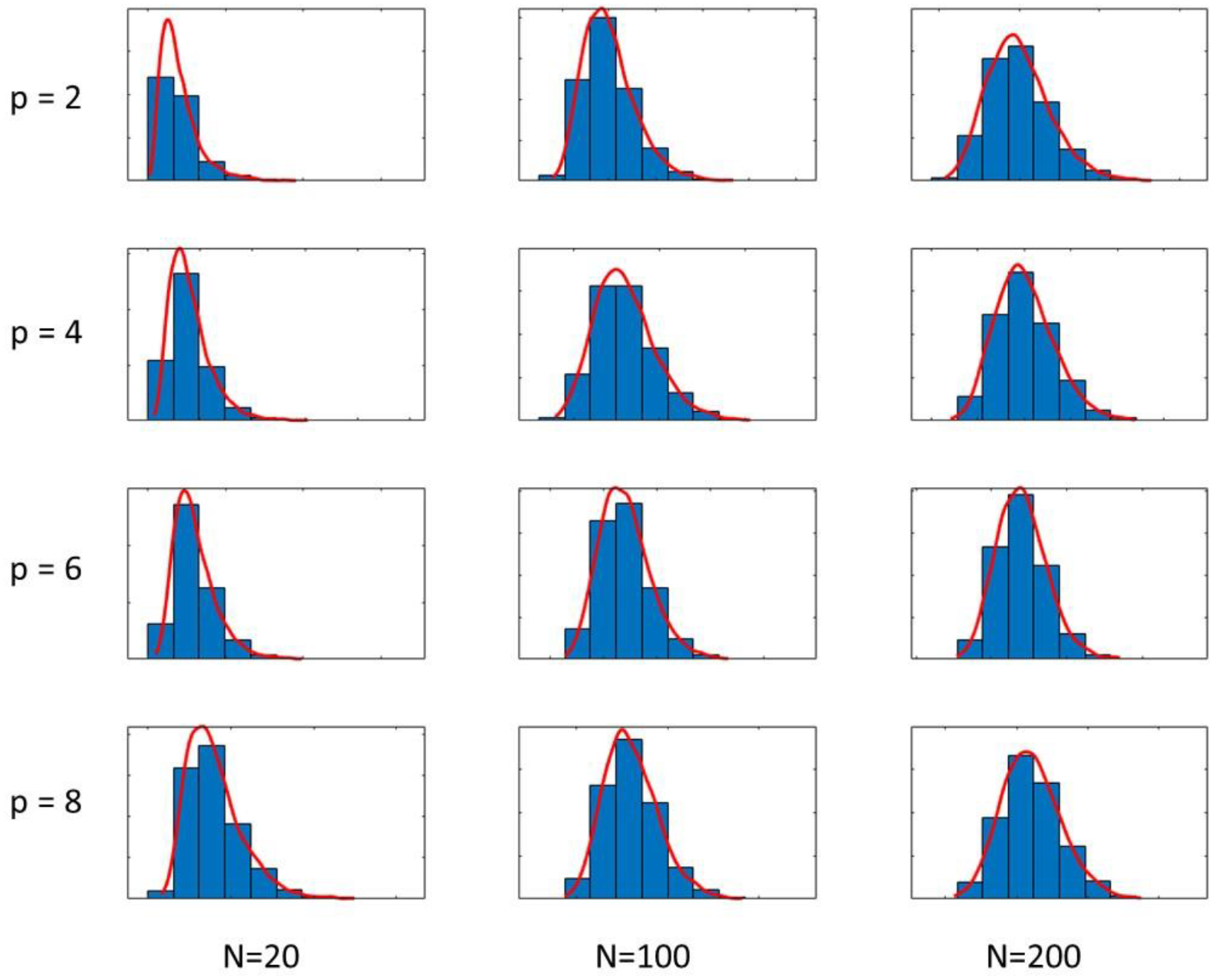
Simulated sample distributions of the mp-QIB variance estimates for different numbers of QIBs (p) and for different sample sizes (N).

9.0. ESSENTIAL CLAIM COMPONENTS FOR A MP-QIB

The claim components that are essential to the entire mp-QIB profile are provided in detail in Supplement 7.

10.0. CASE STUDY

10.1. Background

Alzheimer’s Disease (AD) is characterized by amyloid plaque deposition on several different brain regions as well as neuronal loss resulting in loss of metabolic activity and structural loss of regional and whole brain volume. Guerrero-Gonzalez et al. used the Mahalanobis Distance to classify subjects to a known multivariate distribution¹³⁰ and several authors used multiple imaging QIBs to predict time-to-event^{131, 132}. Sur et al.¹³³ evaluated the change over time due to a BACE inhibitor from six different brain volumes univariately and Schwarz et al. evaluated annualized univariate changes in five regional brain volumes as well as conducting an exploratory analysis of individual structures in four major brain regions¹³⁴. However, to our knowledge, a vector-based estimation of longitudinal change has not been conducted.

One continuing issue for clinical trials is that enrollment has to tread a fine line between enrolling subjects who are actively progressing for the endpoint(s) being evaluated. Enrolling subjects too early in the disease may not progress or see changes in the endpoints during the study duration (placebo), and subjects too late in the disease may not be able to respond to any therapeutic intervention. Additionally, disease progression in AD is noted for several stages that correspond to different endpoints¹³⁵, and uncertainty of the stage upon enrollment makes it difficult to rely on a single QIB. Therefore, using a mp-QIB for a multivariate assessment of AD may overcome the limitations of univariate QIBs.

10.2. Case study data

ADNI includes subjects between the ages of 55 to 90 from institutions in the US and Canada. The ADNI data consists of imaging from multiple modalities as well as other measures of neurodegeneration. This case study used the multiple QIB imaging data from the ADNIADNIMERGE dataset consisting of data from ADNI1, ADNI2, and ADNI GO databases¹³⁶ to extract data from eight QIBs for assessing the effect of AD on the brain. No treatment information is available, and no analysis of treatment effect is conducted. Therefore, the hypotheses to test for the superiority of the mp-QIB, described in Section 7.2, are to measure change in AD over time due to neurodegeneration. No consideration was made for the use of different therapeutic interventions.

As explained in Section 8, there is no mp-QIB measurand; therefore, the mp-QIB will be evaluated for superior sensitivity to measure change over time by comparing the mp-QIB to the univariate QIBs for change from baseline of the Month 24 results. No perceived medical order of importance was assumed for a multiple endpoints assessment, and rejecting the null hypothesis will require significant superiority over all of the QIBs included in the final model.

To download the data and the SAS/R/SPSS code necessary to create the ADNIMERGE data set, the following steps should be taken:

1. Register or log into the IDA.LONI.USC.EDU website;

2. Go to the “Download Study Data” tab;

3. Choose “Study Info” on the menu and choose “Data & Database;”

4. Choose the appropriate method, SAS/R/SPSS/Stata, for downloading the data and the code for merging the data sets; and

5. Run the code to create the ADNIMERGE dataset.

10.3. Subject Selection

The inclusion criteria consisted of all ADNIMERGE subjects with any diagnosis who had Baseline and Month 24 scans for both PET and MRI. Subjects with no MRI scans data were not included. Missing QIBs for either visit were imputed using multiple imputation procedures in SAS Ver. 9.4. The following four diagnostic subgroups were used in the mp-QIB development:

• Cognitively Normal (CN);

• Early Mild Cognitive Impairment (EMCI);

• Late Mild Cognitive Impairment (LMCI); and

• Alzheimer’s Disease (AD).

The QIB initial candidate pool consisted of all QIBs within the data set except for intracranial volume (ICV), which is not expected to change. The QIBs included the following: FDG-PET, Amyloid PET (AV45), and structural MRI volumes for the entorhinal cortex, fusiform gyrus, middle temporal, ventricles, hippocampus, and whole brain. Covariables such as age, race, gender, ICV, and ApoE4 status were not considered in this analysis, but if included in a linear model, the QIB covariance for each subgroup would be estimated from a mixed effects model with repeated measures. Each QIB was determined to have a right-skewed distribution, and the log transform was used for multiple imputation, EFA and CFA, and mp-QIB calculation. A summary depiction of the workflow followed in this case study is found in Figure 5.

Figure 5.

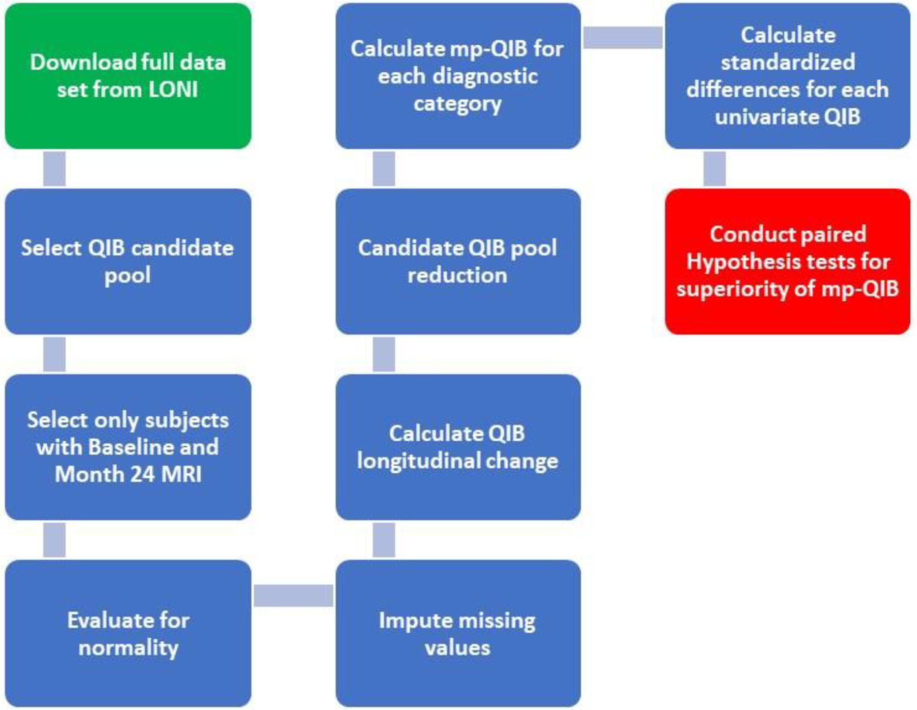
Case Study Workflow to develop a mp-QIB

The EFA was conducted for each of the seven imputation runs. The mean factor loadings used to reduce the QIB candidate set to four QIBs as component QIBs and two factors as latent constructs of neurodegeneration. The baseline diagnoses were used to identify different stages of the disease; however, if the intended population for the mp-QIB extends from CN to AD, then the mp-QIB workflow should also consider using all subjects as one group. The EFA used the Procrustes method of rotation. Other methods, such as Varimax, had similar results.

10.4. Results

Using all subjects and diagnoses, the EFA identified two factors that explained almost all of the total variance (See Figure 6). The loading threshold of 0.4 was used in this illustrative example to allow for at least two QIBs per factor. However, there is no universal rule for an appropriate threshold, and one should be chosen based on the QIBs being evaluated, the number of latent disease constructs expected, and the intended use of the mp-QIB.

Figure 6.

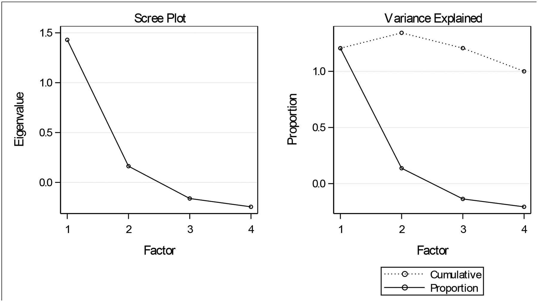
Scree plot for the multivariate Exploratory Factor Analysis identifying 2 major factors

The final path diagram is shown in Figure 7. Ventricle and Whole Brain volumes were chosen to define Factor 1 and Entorhinal and Fusiform volumes to define Factor 2. There is also a considerable correlation between factors (ρ(F1,F2) = 0.7) which is consistent with the progression stages of dementia related to AD¹³⁵. The comparison of the mp-QIB to the standardized differences, also known as the effect sizes, for each QIB is shown in Figure 8 and also in Supplement 8 for paired QIB-to-mp-QIB comparisons. SAS^® and MATLAB^™ code used in this case study are provided in Supplements 9 and 10.

Figure 7.

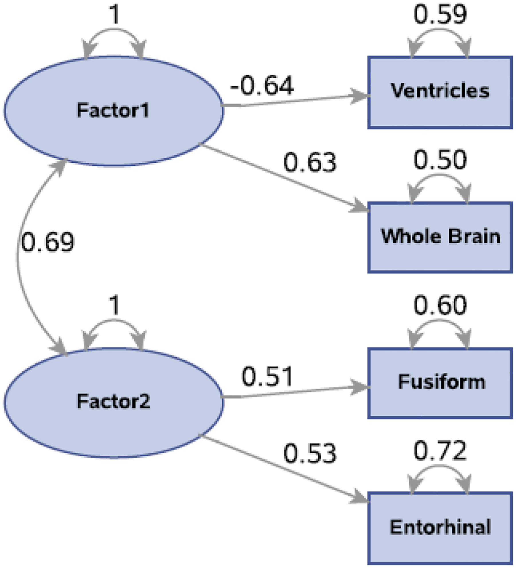
Path analysis for the final mp-QIB model

Figure 8.

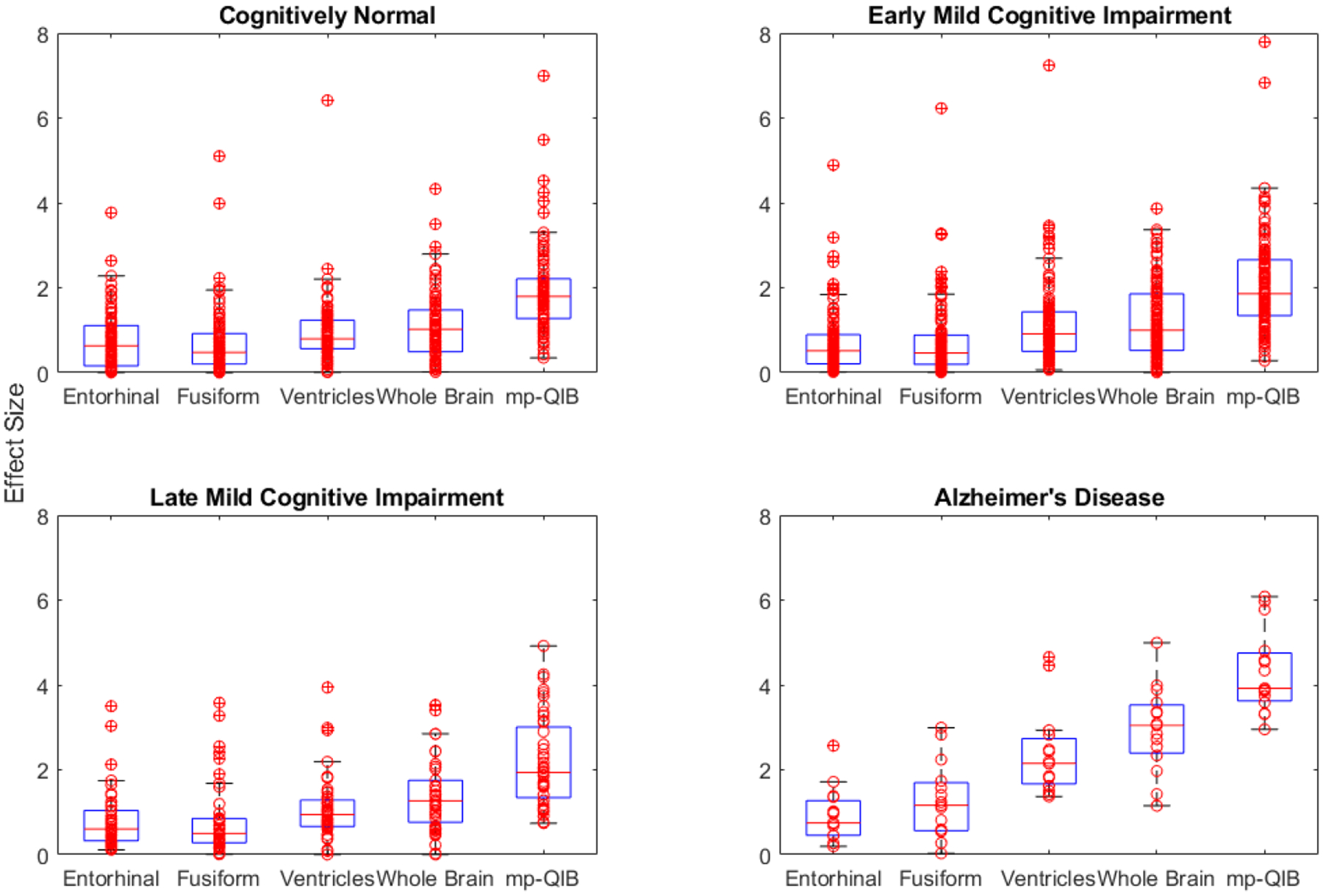
Box plots of DM effect size and individual QIB effect sizes for (a) Cognitively Normal, (b) Mild Cognitive Impairment and (c) Alzheimer’s Disease subjects.

The model fit statistics reviewed in this case study were goodness of fit index (GFI), absolute root mean square error (RMSEA), and Standardized residual root mean square (SRMR) since they provide more accurate information on goodness-of-fit¹⁰⁴. The results indicate that the overall goodness of fit is good (GFI = 0.9), and the RMSEA estimate is larger than 0.05, possibly due to the imbalance of subjects between CN/EMCI/LMCI and AD and to transformed QIB distributions that are not quite normal, which would also affect the imputed variables.

The paired comparisons, however, are all highly significant (p<0.001), even when adjusting for multiple QIB comparisons. In addition, all subjects for all QIBs had mp-QIB effect size values larger than the univariate QIB effect sizes.

10.5. Case Study Conclusion

The mp-QIB absolute effect sizes are significantly larger than all univariate QIB effect sizes for each baseline diagnosis provided in the ADNIMERGE data set. In addition, multiple imputation allowed for all subjects who had a scan at both baseline and Month 24 but had a missing QIB to be included in the evaluation of the model as well as the estimation of the mp-QIB without the default casewise deletion that can occur in multivariate modeling.

11.0. DISCUSSION

In many if not most diseases, univariate measurements do not entirely describe the disease or overall assessment of efficacy¹³, leading the way to the using multiple endpoints and multivariate models. Multiple endpoints are often used because there is little consensus in many diseases on which of the biomarkers is most important, or even if there is a primary signal of disease response to treatment¹⁶. Furthermore, different disease manifestations add to the entire complexity of assessing changes in the disease due to treatments that can affect endpoints upstream and downstream of the primary mechanism of action.

The use of imaging in the description of many diseases has expanded beyond measuring size to evaluating morphological evolution, texture, and cellular function. For example, oncology imaging now includes both function and texture in response to more complex treatments^17–20. The evolution of cardiac imaging also now includes multiple estimates of size, tissue characterization, and cardiac function^22–25. Additionally, cardiovascular plaque evolved from simple measures of carotid intima-media thickness and luminal diameter to a full tissue characterization of the arterial plaque^26–28.

Though all well-designed studies attempt to enroll a homogeneous subject population., inclusion criteria are very often necessarily broad for practical reasons. They often rely on imprecise criteria to accommodate enrollment. Therefore, different disease constructs may be involved at different times within the same clinical trial. A multivariate measure of disease could better accommodate the necessities of a less-than-homogeneous enrollment population.

Combining QIBs into a single determination of longitudinal change has been primarily limited to using multiple endpoints evaluated or as a composite endpoint for staging, disease categorization, or risk^{17, 31–38}. The mp-QIB concept as a vector of QIBs has much in common with AI systems. The mp-QIB and an AI-based bioinformatics model both use a pool of QIBs to develop a final set of univariate QIBs that, together, better predict treatment effect on the clinical outcome than any single QIB. However, the mp-QIB explicitly measures the disease by the defining vector function, while the AI model uses the QIBs to define a model that measures similarity to a known disease state. Even for a specified intended use, the AI function could be modified by different or additional training sets, while the component QIBs explicitly define the mp-QIB.

12.0. CONCLUSIONS

mp-QIBs overcome some intractable limitations of univariate QIBs and are better suited to evaluating complex diseases more comprehensively. As the ADNI collection of imaging data for AD research importantly includes objective measures of brain size as well as measures of connectivity, functional activity, and perfusion it was ideal in our use case for representing neurodegeneration more globally in AD. In clinical trials, the particular state of AD at any one time is not known with any precision due to the overlapping pathophysiologies of dementia¹³³, which further exacerbates the problem of assessing neurodegeneration. This ambiguity in longitudinal disease progression seen in AD is arguably true for many other diseases. Fortunately, the impact of using mp-QIBs, particularly in complex disease, is that not only can an inference be made on the sample but also that each subject can be evaluated simultaneously for all of the biomarkers at a point in time, overcoming the severe and intractable limitations of several single QIBs, that are inadequately modelled.

The mp-QIB represents a vector-based method of simultaneously evaluating multiple constructs that form the overall etiology of a disease. Development of the mp-QIB, except for dimension reduction, follows the same concepts of technical performance for univariate disease for repeatability and reproducibility. While the steps to quantify technical performance require some additional considerations beyond those for univariate QIBs, the use of validly profiled QIBs as components offers the opportunity to reduce reliance on multiple comparisons adjustment decisions, hierarchical ordering of QIB importance, or ad hoc composite endpoint creation. It also provides an all-inclusive biomarker value for each subject.

List of Abbreviations

AD

Alzheimer’s disease

ADNI

Alzheimer’s Disease Neuroimaging Initiative

AI

Artificial intelligence

BLOQ

Below the lower limit of quantification

CCC

Concordance correlation coefficient

CFA

Confirmatory factor analysis

CN

Cognitively normal

CT

Computed tomography

DCE-MRI

Dynamic contrast enhanced MRI

DECT

Dual energy computed tomography

DF_n

Kurtosis corrected degrees of freedom

DM

Mahalanobis distance

DM2

Mahalanobis distance squared

DSC

Dynamic susceptibility contrast imaging

DTI

Diffusion tensor imaging

DX

X₂-X₁

E[X]

The expected value of X

EFA

Exploratory factor analysis

EMCI

Early mild cognitive impairment

FDA

Food and Drug Administration

FDG

Flurodeoxyglucose

GFI

Goodness of fit index

LLOQ

Lower limit of quantification

LMCI

Late cognitive impairment

LOA

Limits of Agreement

LOQ

Limit of quantification

MANOVA

Multivariate analysis of variance

MANOVA-RM

MANOVA Repeated measures

MAR

Missing at random

MCAR

Missing completely at random

MCCC

Multivariate CCC

MCD

Minimum covariance determinant

MCI

Mild cognitive impairment

mp-QIB

Multiparametric QIB

MRI

Magnetic resonance imaging

PET

Positron emission tomography

QIB

Quantitative Imaging Biomarker

QIBA

Quantitative Imaging Biomarker Alliance

RC

Repeatability coefficient

RC_mp

Multiparametric RC

RDC_mp

Multiparametric reproducibility coefficient

RMSEA

Root mean square error of approximation

S

Sample variance estimate

SAS®

Statistical analysis software

REFERENCES

- 1.Kessler L, Barnhart H, Buckler A, et al. ; QIBA Terminology Working Group. The emerging science of quantitative imaging biomarkers terminology and definitions for scientific studies and regulatory submissions. Stat Methods Med Res 2015; 24: 9–26. [DOI] [PubMed] [Google Scholar]
- 2.QIBA. Quantitative Imaging Biomarkers Alliance (QIBA), https://qibawiki.rsna.org/index.php/Main_Page (2021, accessed July 6, 2021).
- 3.Raunig DL, McShane LM, Pennello G, et al. Quantitative imaging biomarkers: a review of statistical methods for technical performance assessment. Statistical methods in medical research 2015; 24: 27–67. [DOI] [PMC free article] [PubMed] [Google Scholar]
- 4.Sullivan DC, Obuchowski NA, Kessler LG, et al. Metrology standards for quantitative imaging biomarkers. Radiology 2015; 277: 813–825. [DOI] [PMC free article] [PubMed] [Google Scholar]
- 5.Obuchowski NA, Reeves AP, Huang EP, et al. Quantitative imaging biomarkers: a review of statistical methods for computer algorithm comparisons. Statistical methods in medical research 2015; 24: 68–106. [DOI] [PMC free article] [PubMed] [Google Scholar]
- 6.Huang EP, Wang X-F, Choudhury KR, et al. Meta-analysis of the technical performance of an imaging procedure: guidelines and statistical methodology. Statistical methods in medical research 2015; 24: 141–174. [DOI] [PMC free article] [PubMed] [Google Scholar]
- 7.Committee QM. https://qibawiki.rsna.org/index.php/Metrology_Committee.
- 8.Huang EP, Wang X, Pennello G, et al. A Roadmap for Developing and Evaluating Quantitative Imaging Biomarker-Based Models for Risk Prediction. Academic Radiology 2022. Submitted. [Google Scholar]
- 9.Delfino J, Wang X, Pennello G, et al. Multiparametric Quantitative Imaging Biomarkers in Phenotype Classification Academic Radiology 2022. Submitted. [DOI] [PMC free article] [PubMed] [Google Scholar]
- 10.Obuchowski NA, Wang X, Pennello G, et al. Multi-parametric Quantitative Imaging Biomarkers (QIBs): A Framework for Estimating and Testing Technical Performance. Academic Radiology 2022. [Google Scholar]
- 11.Wang X, Pennello G, deSouza N, et al. Multiparametric Data-driven Imaging Markers: Guidelines for Development, Application and Reporting of Model Outputs in Radiomics Academic Radiology 2022. (Submitted). [DOI] [PMC free article] [PubMed] [Google Scholar]
- 12.Biomarkers Definitions Working Group, Atkinson AJ Jr, Colburn WA, et al. Biomarkers and surrogate endpoints: preferred definitions and conceptual framework. Clinical pharmacology & therapeutics 2001; 69: 89–95. [DOI] [PubMed] [Google Scholar]
- 13.O’Brien PC. Procedures for comparing samples with multiple endpoints. Biometrics 1984: 1079–1087. [PubMed] [Google Scholar]
- 14.Adams LC, Bressem KK, Scheibl S, et al. Multiparametric Assessment of Changes in Renal Tissue after Kidney Transplantation with Quantitative MR Relaxometry and Diffusion-Tensor Imaging at 3 T. J Clin Med 2020; 9 2020/05/28. DOI: 10.3390/jcm9051551. [DOI] [PMC free article] [PubMed] [Google Scholar]
- 15.Vamvakas A, Williams SC, Theodorou K, et al. Imaging biomarker analysis of advanced multiparametric MRI for glioma grading. Phys Med 2019; 60: 188–198. 2019/03/27. DOI: 10.1016/j.ejmp.2019.03.014. [DOI] [PubMed] [Google Scholar]
- 16.Sankoh AJ, D’Agostino RB Sr and Huque MF. Efficacy endpoint selection and multiplicity adjustment methods in clinical trials with inherent multiple endpoint issues. Statistics in Medicine 2003; 22: 3133–3150. [DOI] [PubMed] [Google Scholar]
- 17.Cheson BD, Fisher RI, Barrington SF, et al. Recommendations for initial evaluation, staging, and response assessment of Hodgkin and non-Hodgkin lymphoma: the Lugano classification. 2014; 32: 3059. [DOI] [PMC free article] [PubMed] [Google Scholar]
- 18.Galbraith SM, Rustin GJ, Lodge MA, et al. Effects of 5, 6-dimethylxanthenone-4-acetic acid on human tumor microcirculation assessed by dynamic contrast-enhanced magnetic resonance imaging. Journal of clinical oncology 2002; 20: 3826–3840. [DOI] [PubMed] [Google Scholar]
- 19.Nanni C, Cottereau AS, Lopci E, et al. Report of the 6th International Workshop on PET in lymphoma. Leukemia & lymphoma 2017; 58: 2298–2303. [DOI] [PubMed] [Google Scholar]
- 20.Padhani AR and Miles KA. Multiparametric imaging of tumor response to therapy. Radiology 2010; 256: 348–364. [DOI] [PubMed] [Google Scholar]
- 21.Bosca RJ. Methodological development of a multi-parametric quantitative imaging biomarker framework for assessing treatment response with MRI. 2014.
- 22.Heggemann F, Grotz H, Welzel G, et al. Cardiac function after multimodal breast cancer therapy assessed with functional magnetic resonance imaging and echocardiography imaging. International Journal of Radiation Oncology* Biology* Physics 2015; 93: 836–844. [DOI] [PubMed] [Google Scholar]
- 23.Eslami P, Parmar C, Foldyna B, et al. Radiomics of Coronary Artery Calcium in the Framingham Heart Study. Radiology: Cardiothoracic Imaging 2020; 2: e190119. [DOI] [PMC free article] [PubMed] [Google Scholar]
- 24.Biering-Sørensen T and Solomon SD. Assessing contractile function when ejection fraction is normal: a case for strain imaging. Am Heart Assoc, 2015. [DOI] [PubMed] [Google Scholar]
- 25.Selmeryd J, Henriksen E, Dalen H, et al. Derivation and evaluation of age-specific multivariate reference regions to aid in identification of abnormal filling patterns: the HUNT and VaMIS studies. JACC: Cardiovascular Imaging 2018; 11: 400–408. [DOI] [PubMed] [Google Scholar]
- 26.Bots ML, Evans GW, Riley WA, et al. Carotid intima-media thickness measurements in intervention studies: design options, progression rates, and sample size considerations: a point of view. Stroke 2003; 34: 2985–2994. [DOI] [PubMed] [Google Scholar]
- 27.Wan T, Madabhushi A, Phinikaridou A, et al. Spatio- temporal texture (SpTeT) for distinguishing vulnerable from stable atherosclerotic plaque on dynamic contrast enhancement (DCE) MRI in a rabbit model. Medical physics 2014; 41: 042303. [DOI] [PMC free article] [PubMed] [Google Scholar]
- 28.Pierre SS, Siegelman J, Obuchowski NA, et al. Measurement accuracy of atherosclerotic plaque structure on CT using phantoms to establish ground truth. Academic radiology 2017; 24: 1203–1215. [DOI] [PMC free article] [PubMed] [Google Scholar]
- 29.Nir TM, Jahanshad N, Villalon-Reina JE, et al. Effectiveness of regional DTI measures in distinguishing Alzheimer’s disease, MCI, and normal aging. NeuroImage: clinical 2013; 3: 180–195. [DOI] [PMC free article] [PubMed] [Google Scholar]
- 30.Watson C, Busovaca E, Foley JM, et al. White matter hyperintensities correlate to cognition and fiber tract integrity in older adults with HIV. Journal of neurovirology 2017; 23: 422–429. [DOI] [PMC free article] [PubMed] [Google Scholar]
- 31.Choi H, Charnsangavej C, Faria SC, et al. Correlation of computed tomography and positron emission tomography in patients with metastatic gastrointestinal stromal tumor treated at a single institution with imatinib mesylate: proposal of new computed tomography response criteria. Journal of Clinical Oncology 2007; 25: 1753–1759. [DOI] [PubMed] [Google Scholar]
- 32.Veale D, Reece R, Parsons W, et al. Intra-articular primatised anti-CD4: efficacy in resistant rheumatoid knees. A study of combined arthroscopy, magnetic resonance imaging, and histology. Annals of the rheumatic diseases 1999; 58: 342–349. [DOI] [PMC free article] [PubMed] [Google Scholar]
- 33.Nachimuthu DS and Baladhandapani A. Multidimensional texture characterization: on analysis for brain tumor tissues using MRS and MRI. Journal of digital imaging 2014; 27: 496–506. [DOI] [PMC free article] [PubMed] [Google Scholar]
- 34.Murgia A, Balestrieri A, Francone M, et al. Plaque imaging volume analysis: technique and application. Cardiovascular Diagnosis and Therapy 2020; 10: 1032. [DOI] [PMC free article] [PubMed] [Google Scholar]
- 35.Sheahan M, Ma X, Paik D, et al. Atherosclerotic plaque tissue: noninvasive quantitative assessment of characteristics with software-aided measurements from conventional CT angiography. Radiology 2018; 286: 622–631. [DOI] [PMC free article] [PubMed] [Google Scholar]
- 36.Barrington SF, Mikhaeel NG, Kostakoglu L, et al. Role of imaging in the staging and response assessment of lymphoma: consensus of the International Conference on Malignant Lymphomas Imaging Working Group. J Clin Oncol 2014; 32: 3048–3058. 2014/08/11. DOI: 10.1200/JCO.2013.53.5229. [DOI] [PMC free article] [PubMed] [Google Scholar]
- 37.Nishiyama KK and Shane E. Clinical imaging of bone microarchitecture with HR-pQCT. Current osteoporosis reports 2013; 11: 147–155. [DOI] [PMC free article] [PubMed] [Google Scholar]
- 38.Si Y, Merz SF, Jansen P, et al. Multidimensional imaging provides evidence for down-regulation of T cell effector function by MDSC in human cancer tissue. Science immunology 2019; 4. [DOI] [PubMed] [Google Scholar]
- 39.US Food and Drug Administration. Multiple Endpoints in Clinical Trials Guidance for Industry Draft Guidance. Washington, DC: 2017. [Google Scholar]
- 40.Fleming TR and Powers JH. Biomarkers and surrogate endpoints in clinical trials. Statistics in medicine 2012; 31: 2973–2984. [DOI] [PMC free article] [PubMed] [Google Scholar]
- 41.Zemans RL, Jacobson S, Keene J, et al. Multiple biomarkers predict disease severity, progression and mortality in COPD. Respiratory Research 2017; 18: 117. DOI: 10.1186/s12931-017-0597-7. [DOI] [PMC free article] [PubMed] [Google Scholar]
- 42.Offen W, Chuang-Stein C, Dmitrienko A, et al. Multiple Co-primary Endpoints: Medical and Statistical Solutions A Report From the Multiple Endpoints Expert Team of the Pharmaceutical Research and Manufacturers of America. Drug Information Journal 2007; 41: 31. [Google Scholar]
- 43.QIBA. QIBA Profile Claim Guidance, http://qibawiki.rsna.org/index.php/Claim_Guidance (2021, accessed 03/16/2021 2921).
- 44.Offen WW and Helterbrand JD. Multiple comparison adjustments when two or more co-primary endpoints must all be statistically significant. In: Proceedings of the Annual Meeting of the American Statistical Association, Chicago, IL 1986. [Google Scholar]
- 45.Chuang- Stein C, Stryszak P, Dmitrienko A, et al. Challenge of multiple co-primary endpoints: a new approach. Statistics in medicine 2007; 26: 1181–1192. [DOI] [PubMed] [Google Scholar]
- 46.Chuang-stein C, Dmitrienko A and Offen W. Discussion of “Some Controversial Multiple Testing Problems in Regulatory Applications”. Journal of Biopharmaceutical Statistics 2009; 19: 14–21. DOI: 10.1080/10543400802541719. [DOI] [PubMed] [Google Scholar]
- 47.Offen W, Chuang-Stein C, Dmitrienko A, et al. Multiple co-primary endpoints: medical and statistical solutions: a report from the multiple endpoints expert team of the Pharmaceutical Research and Manufacturers of America. Drug information journal 2007; 41: 31–46. [Google Scholar]
- 48.Dmitrienko A and Tamhane AC. Gatekeeping procedures with clinical trial applications. Pharmaceutical Statistics: The Journal of Applied Statistics in the Pharmaceutical Industry 2007; 6: 171–180. [DOI] [PubMed] [Google Scholar]
- 49.Pocock SJ, Geller NL and Tsiatis AA. The analysis of multiple endpoints in clinical trials. Biometrics 1987: 487–498. [PubMed] [Google Scholar]
- 50.Cordoba G, Schwartz L, Woloshin S, et al. Definition, reporting, and interpretation of composite outcomes in clinical trials: systematic review. BMJ 2010; 341. [DOI] [PMC free article] [PubMed] [Google Scholar]
- 51.Boers M, Tugwell P, Felson D, et al. World Health Organization and International League of Associations for Rheumatology core endpoints for symptom modifying antirheumatic drugs in rheumatoid arthritis clinical trials. The Journal of rheumatology Supplement 1994; 41: 86–89. [PubMed] [Google Scholar]
- 52.Stevens SR, Ke MS, Parry EJ, et al. Quantifying skin disease burden in mycosis fungoides–type cutaneous T-cell lymphomas: the Severity-Weighted Assessment Tool (SWAT). Archives of dermatology 2002; 138: 42–48. [DOI] [PubMed] [Google Scholar]
- 53.Olsen EA, Kim YH, Kuzel TM, et al. Phase IIb multicenter trial of vorinostat in patients with persistent, progressive, or treatment refractory cutaneous T-cell lymphoma. Journal of clinical oncology 2007; 25: 3109–3115. [DOI] [PubMed] [Google Scholar]
- 54.Armstrong PW and Westerhout CM. Composite end points in clinical research: a time for reappraisal. Circulation 2017; 135: 2299–2307. [DOI] [PubMed] [Google Scholar]
- 55.Buyse M, Molenberghs G, Paoletti X, et al. Statistical evaluation of surrogate endpoints with examples from cancer clinical trials. Biometrical Journal 2016; 58: 104–132. [DOI] [PubMed] [Google Scholar]
- 56.Evans SR, Rubin D, Follmann D, et al. Desirability of outcome ranking (DOOR) and response adjusted for duration of antibiotic risk (RADAR). Clinical Infectious Diseases 2015; 61: 800–806. [DOI] [PMC free article] [PubMed] [Google Scholar]
- 57.Finkelstein DM and Schoenfeld DA. Combining mortality and longitudinal measures in clinical trials. Statistics in medicine 1999; 18: 1341–1354. [DOI] [PubMed] [Google Scholar]
- 58.Buyse M Generalized pairwise comparisons of prioritized outcomes in the two-sample problem. Statistics in medicine 2010; 29: 3245–3257. [DOI] [PubMed] [Google Scholar]
- 59.Pocock SJ, Ariti CA, Collier TJ, et al. The win ratio: a new approach to the analysis of composite endpoints in clinical trials based on clinical priorities. European heart journal 2012; 33: 176–182. [DOI] [PubMed] [Google Scholar]
- 60.Sun H, Davison BA, Cotter G, et al. Evaluating treatment efficacy by multiple end points in phase II acute heart failure clinical trials: analyzing data using a global method. Circulation: Heart Failure 2012; 5: 742–749. [DOI] [PubMed] [Google Scholar]
- 61.Berry JD, Miller R, Moore DH, et al. The Combined Assessment of Function and Survival (CAFS): a new endpoint for ALS clinical trials. Amyotrophic lateral sclerosis and frontotemporal degeneration 2013; 14: 162–168. [DOI] [PubMed] [Google Scholar]
- 62.Doernberg SB, Tran TTT, Tong SY, et al. Good studies evaluate the disease while great studies evaluate the patient: development and application of a desirability of outcome ranking endpoint for Staphylococcus aureus bloodstream infection. Clinical Infectious Diseases 2019; 68: 1691–1698. [DOI] [PMC free article] [PubMed] [Google Scholar]
- 63.Phillips PPJ, Morris TP and Walker AS. DOOR/RADAR: A Gateway Into the Unknown? Clinical infectious diseases: an official publication of the Infectious Diseases Society of America 2016; 62: 814–815. [DOI] [PubMed] [Google Scholar]
- 64.Follmann D, Fay MP, Hamasaki T, et al. Analysis of ordered composite endpoints. Statistics in Medicine 2020; 39: 602–616. [DOI] [PMC free article] [PubMed] [Google Scholar]
- 65.Johnson RA and Wichern DW. Applied multivariate statistical analysis. Pearson; London, UK:, 2014. [Google Scholar]
- 66.Wiemker R, Bergtholdt M, Dharaiya E, et al. Agreement of CAD features with expert observer ratings for characterization of pulmonary nodules in CT using the LIDC-IDRI database. In: Medical Imaging 2009: Computer-Aided Diagnosis 2009, p.72600H. International Society for Optics and Photonics. [Google Scholar]
- 67.Jiang J, Wang M, Alberts I, et al. Using radiomics-based modelling to predict individual progression from mild cognitive impairment to Alzheimer’s disease. European Journal of Nuclear Medicine and Molecular Imaging 2022: 1–11. [DOI] [PubMed] [Google Scholar]
- 68.Little R, D’Agostino R, Dickersin K, et al. The Prevention and Treatment of Missing Data in Clinical Trials. Pannel on Handling Missing Data in Clinical Trials. 2010. [Google Scholar]
- 69.Borman PJ and Chatfield MJ. Avoid the perils of using rounded data. Journal of Pharmaceutical and Biomedical Analysis 2015; 115: 502–508. [DOI] [PubMed] [Google Scholar]
- 70.Box GE and Cox DR. An analysis of transformations. Journal of the Royal Statistical Society: Series B (Methodological) 1964; 26: 211–243. [Google Scholar]
- 71.Wayne D. CLSI Evaluation of Detection Capability for Clinical Laboratory Measurement Procedures; Approved Guideline. CLSI document EP17-A2. Clinical and Laboratory Standards Institute, 2012. [Google Scholar]
- 72.Liao SG, Lin Y, Kang DD, et al. Missing value imputation in high-dimensional phenomic data: imputable or not, and how? BMC Bioinformatics 2014; 15: 346. 2014/11/06. DOI: 10.1186/s12859-014-0346-6. [DOI] [PMC free article] [PubMed] [Google Scholar]
- 73.Schafer JL. Multiple imputation: a primer. Statistical methods in medical research 1999; 8: 3–15. [DOI] [PubMed] [Google Scholar]
- 74.Little RJ and Rubin DB. Statistical analysis with missing data. John Wiley & Sons, 2019. [Google Scholar]
- 75.Wang Z, Akande O, Poulos J, et al. Are deep learning models superior for missing data imputation in large surveys? Evidence from an empirical comparison. arXiv preprint arXiv:210309316 2021. [Google Scholar]
- 76.Jiang X, Hintenlang DE and White RD. Lower limit of iron quantification using dual- energy CT—a phantom study. Journal of Applied Clinical Medical Physics 2021; 22: 299–307. [DOI] [PMC free article] [PubMed] [Google Scholar]
- 77.Kremkau FW. Sonography Principles and Instruments E-Book. Elsevier Health Sciences, 2019. [Google Scholar]
- 78.Baba T Evaluation of Post Wall Filter for Doppler Ultrasound Systems. Acoustical Imaging. Springer, 2008, pp.133–138. [Google Scholar]
- 79.Guo Y, Harel O and Little RJ. How well quantified is the limit of quantification? Epidemiology 2010: S10–S16. [DOI] [PubMed] [Google Scholar]
- 80.Lyles RH, Fan D and Chuachoowong R. Correlation coefficient estimation involving a left censored laboratory assay variable. Statistics in Medicine 2001; 20: 2921–2933. [DOI] [PubMed] [Google Scholar]
- 81.Barnett HY, Geys H, Jacobs T, et al. Methods for Non-Compartmental Pharmacokinetic Analysis With Observations Below the Limit of Quantification. Statistics in Biopharmaceutical Research 2021; 13: 59–70. [Google Scholar]
- 82.Zhou H, Hartford A and Tsai K. A Bayesian Approach for PK/PD Modeling with PD Data Below Limit of Quantification. Journal of Biopharmaceutical Statistics 2012; 22: 1220–1243. DOI: 10.1080/10543406.2011.585441. [DOI] [PubMed] [Google Scholar]
- 83.Senn S, Holford N and Hockey H. The ghosts of departed quantities: approaches to dealing with observations below the limit of quantitation. Statistics in medicine 2012; 31: 4280–4295. [DOI] [PubMed] [Google Scholar]
- 84.Herbers J, Miller R, Walther A, et al. How to deal with non-detectable and outlying values in biomarker research: Best practices and recommendations for univariate imputation approaches. Comprehensive Psychoneuroendocrinology 2021; 7: 100052. [DOI] [PMC free article] [PubMed] [Google Scholar]
- 85.Harel O, Perkins N and Schisterman EF. The Use of Multiple Imputation for Data Subject to Limits of Detection. Sri Lankan J Appl Stat 2014; 5: 227–246. 2014/12/15. DOI: 10.4038/sljastats.v5i4.7792. [DOI] [PMC free article] [PubMed] [Google Scholar]
- 86.Nassiri V, Barnett H, Geys H, et al. BLOQ: Impute and Analyze Data With Observations Below the Limit of Quantification, https://cran.r-project.org/web/packages/BLOQ/ (2018).
- 87.Williams JR, Kim H-W and Crespi CM. Modeling observations with a detection limit using a truncated normal distribution with censoring. BMC Medical Research Methodology 2020; 20: 170. DOI: 10.1186/s12874-020-01032-9. [DOI] [PMC free article] [PubMed] [Google Scholar]
- 88.US Food and Drug Administration. Technical Performance Assessment of Quantitative Imaging in Radiological Device Premarket Submissions Guidance for Industry and Food and Drug Administration Staff. In: Center for Devices and Radiological Health, (ed.). Silver Spring, MD: June 16, 2022. [Google Scholar]
- 89.Taouli B, Ehman RL and Reeder SB. Advanced MRI Methods for Assessment of Chronic Liver Disease. American Journal of Roentgenology 2009; 193: 14–27. DOI: 10.2214/AJR.09.2601. [DOI] [PMC free article] [PubMed] [Google Scholar]
- 90.Harrell FE. Regression modeling strategies: with applications to linear models, logistic and ordinal regression, and survival analysis. Springer, 2015. [Google Scholar]
- 91.Madukaife MS. Use of the theory of Euclidean distance in testing for multivariate normality with application to breast cancer diagnostic data. 2020.
- 92.Wang F, Xiang X, Cheng J, et al. Normface: L2 hypersphere embedding for face verification. In: Proceedings of the 25th ACM international conference on Multimedia 2017, pp.1041–1049. [Google Scholar]
- 93.Kullback S and Leibler RA. On Information and Sufficiency. The Annals of Mathematical Statistics 1951; 22: 79–86, 78. [Google Scholar]
- 94.Rao CR. Tests of significance in multivariate analysis. Biometrika 1948; 35: 58–79. [PubMed] [Google Scholar]
- 95.Huberty CJ. Mahalanobis distance. Wiley StatsRef: Statistics Reference Online 2014. [Google Scholar]
- 96.Johnson NL, Kotz S and Johnson NL. Continuous univariate distributions. 1994; 1: 451. [Google Scholar]
- 97.Knuth DE. Art of computer programming, volume 2: Seminumerical algorithms. Addison-Wesley Professional, 2014. [Google Scholar]
- 98.Davatzikos C, Rathore S, Bakas S, et al. Cancer imaging phenomics toolkit: quantitative imaging analytics for precision diagnostics and predictive modeling of clinical outcome. Journal of medical imaging 2018; 5: 011018. [DOI] [PMC free article] [PubMed] [Google Scholar]
- 99.Ahmad OF, Mori Y, Misawa M, et al. Establishing key research questions for the implementation of artificial intelligence in colonoscopy: a modified Delphi method. Endoscopy 2021; 53: 893–901. [DOI] [PMC free article] [PubMed] [Google Scholar]
- 100.Katragadda C, Finnane A, Soyer HP, et al. Technique Standards for Skin Lesion Imaging: A Delphi Consensus Statement. JAMA Dermatology 2017; 153: 207–213. DOI: 10.1001/jamadermatol.2016.3949. [DOI] [PubMed] [Google Scholar]
- 101.Scheltema M, Tay K, Postema A, et al. Utilization of multiparametric prostate magnetic resonance imaging in clinical practice and focal therapy: report from a Delphi consensus project. World journal of urology 2017; 35: 695–701. [DOI] [PMC free article] [PubMed] [Google Scholar]
- 102.DeVellis RF. Scale development: Theory and applications. Sage publications, 2016. [Google Scholar]
- 103.Joliffe IT and Morgan B. Principal component analysis and exploratory factor analysis. Statistical methods in medical research 1992; 1: 69–95. [DOI] [PubMed] [Google Scholar]
- 104.Hatcher L and O’Rourke N. A step-by-step approach to using SAS for factor analysis and structural equation modeling. Sas Institute, 2013. [Google Scholar]
- 105.Anderson JC and Gerbing DW. Structural equation modeling in practice: A review and recommended two-step approach. Psychological bulletin 1988; 103: 411. [Google Scholar]
- 106.Lin J and Bentler PM. A Third Moment Adjusted Test Statistic for Small Sample Factor Analysis. Multivariate Behavioral Research 2012; 47: 448–462. DOI: 10.1080/00273171.2012.673948. [DOI] [PMC free article] [PubMed] [Google Scholar]
- 107.Browne MW. Asymptotically distribution- free methods for the analysis of covariance structures. British journal of mathematical and statistical psychology 1984; 37: 62–83. [DOI] [PubMed] [Google Scholar]
- 108.Wiens BL and Dmitrienko A. On selecting a multiple comparison procedure for analysis of a clinical trial: fallback, fixed sequence, and related procedures. Statistics in Biopharmaceutical Research 2010; 2: 22–32. [Google Scholar]
- 109.Hung HJ and Wang S-J. Some controversial multiple testing problems in regulatory applications. Journal of biopharmaceutical statistics 2009; 19: 1–11. [DOI] [PubMed] [Google Scholar]
- 110.Hollander M, Wolfe DA and Chicken E. Nonparametric statistical methods. John Wiley & Sons, 2013. [Google Scholar]
- 111.Petersen RC, Aisen PS, Beckett LA, et al. Alzheimer’s Disease Neuroimaging Initiative (ADNI): clinical characterization. Neurology 2010; 74: 201–209. 2009/12/30. DOI: 10.1212/WNL.0b013e3181cb3e25. [DOI] [PMC free article] [PubMed] [Google Scholar]
- 112.MacCallum RC, Widaman KF, Zhang S, et al. Sample size in factor analysis. Psychological methods 1999; 4: 84. [Google Scholar]
- 113.Kohl M and Kolampally S. mpe: Multiple Primary Endpoints. 2017.
- 114.Yang S, Moerbeek M, Taljaard M, et al. Power analysis for cluster randomized trials with continuous co-primary endpoints. arXiv preprint arXiv:211201981 2021. [DOI] [PMC free article] [PubMed] [Google Scholar]
- 115.Rencher AC. A review of “Methods of Multivariate Analysis, ”. Taylor & Francis, 2005, p. 558–559. [Google Scholar]
- 116.Hubert M, Debruyne M and Rousseeuw PJ. Minimum covariance determinant and extensions. Wiley Interdisciplinary Reviews: Computational Statistics 2018; 10: e1421. [Google Scholar]
- 117.Rao CR. Generalized inverse of a matrix and its applications. Vol 1 Theory of Statistics. University of California Press, 1972, pp.601–620. [Google Scholar]
- 118.Ben-Israel A and Greville TN. Generalized inverses: theory and applications. Springer Science & Business Media, 2003. [Google Scholar]
- 119.Rousseeuw PJ and Driessen KV. A fast algorithm for the minimum covariance determinant estimator. Technometrics 1999; 41: 212–223. [Google Scholar]
- 120.Lin H, Sardana M, Zhang Y, et al. Association of Habitual Physical Activity with Cardiovascular Disease Risk. Circulation Research 2020. [DOI] [PMC free article] [PubMed] [Google Scholar]
- 121.Hiriote S and Chinchilli VM. Matrix- based concordance correlation coefficient for repeated measures. Biometrics 2011; 67: 1007–1016. [DOI] [PubMed] [Google Scholar]
- 122.Brown MB and Forsythe AB. Robust tests for the equality of variances. Journal of the American Statistical Association 1974; 69: 364–367. [Google Scholar]
- 123.O’Brien PC. Robust procedures for testing equality of covariance matrices. Biometrics 1992: 819–827. [Google Scholar]
- 124.Tiku M and Balakrishnan N. Testing the equality of variance-covariance matrices the robust way. Communications in Statistics-Theory and Methods 1985; 14: 3033–3051. [Google Scholar]
- 125.BIPM I, IFCC, ILAC, IUPAC, IUPAP, ISO, OIML. The international vocabulary of metrology—basic and general concepts and associated terms (VIM, 3rd Edition). JCGM; 200:2012, 2012. [Google Scholar]
- 126.Schott JR. Some tests for the equality of covariance matrices. Journal of Statistical Planning and Inference 2001; 94: 25–36. [Google Scholar]
- 127.Garcia C A simple procedure for the comparison of covariance matrices. BMC Evolutionary Biology 2012; 12: 222. DOI: 10.1186/1471-2148-12-222. [DOI] [PMC free article] [PubMed] [Google Scholar]
- 128.Cho E and Cho MJ. Variance of sample variance. Section on Survey Research Methods–JSM 2008; 2: 1291–1293. [Google Scholar]
- 129.O’Neill B Some useful moment results in sampling problems. The American Statistician 2014; 68: 282–296. [Google Scholar]
- 130.Guerrero-Gonzalez JM, Yeske B, Kirk GR, et al. Mahalanobis distance tractometry (MaD-Tract)–a framework for personalized white matter anomaly detection applied to TBI. NeuroImage 2022; 260: 119475. [DOI] [PMC free article] [PubMed] [Google Scholar]
- 131.Kang K, Pan D and Song X. A joint model for multivariate longitudinal and survival data to discover the conversion to Alzheimer’s disease. Statistics in Medicine 2022; 41: 356–373. [DOI] [PubMed] [Google Scholar]
- 132.Lin J, Li K and Luo S. Functional survival forests for multivariate longitudinal outcomes: Dynamic prediction of Alzheimer’s disease progression. Statistical methods in medical research 2021; 30: 99–111. [DOI] [PMC free article] [PubMed] [Google Scholar]
- 133.Sur C, Kost J, Scott D, et al. BACE inhibition causes rapid, regional, and non-progressive volume reduction in Alzheimer’s disease brain. Brain 2020; 143: 3816–3826. [DOI] [PMC free article] [PubMed] [Google Scholar]
- 134.Schwarz AJ, Sundell KL, Charil A, et al. Magnetic resonance imaging measures of brain atrophy from the EXPEDITION3 trial in mild Alzheimer’s disease. Alzheimer’s & Dementia: Translational Research & Clinical Interventions 2019; 5: 328–337. [DOI] [PMC free article] [PubMed] [Google Scholar]
- 135.Jack CR Jr, Knopman DS, Jagust WJ, et al. Tracking pathophysiological processes in Alzheimer’s disease: an updated hypothetical model of dynamic biomarkers. The lancet neurology 2013; 12: 207–216. [DOI] [PMC free article] [PubMed] [Google Scholar]
- 136.Imaging & Data Archive at the Laboratory of Neuroimging (LONI). ADNI Study Data: ADNIMERGE, https://ida.loni.usc.edu/pages/access/studyData.jsp (accessed June 23, 2022).
Associated Data
This section collects any data citations, data availability statements, or supplementary materials included in this article.