In vivo magnetic resonance ${}^{31}$P‐Spectral Analysis With Neural Networks: 31P‐SPAWNN

Abstract

Purpose

We have introduced an artificial intelligence framework, 31P‐SPAWNN, in order to fully analyze phosphorus‐31 (${}^{31}$P) magnetic resonance spectra. The flexibility and speed of the technique rival traditional least‐square fitting methods, with the performance of the two approaches, are compared in this work.

Theory and Methods

Convolutional neural network architectures have been proposed for the analysis and quantification of ${}^{31}$P‐spectroscopy. The generation of training and test data using a fully parameterized model is presented herein. In vivo unlocalized free induction decay and three‐dimensional ${}^{31}$P‐magnetic resonance spectroscopy imaging data were acquired from healthy volunteers before being quantified using either 31P‐SPAWNN or traditional least‐square fitting techniques.

Results

The presented experiment has demonstrated both the reliability and accuracy of 31P‐SPAWNN for estimating metabolite concentrations and spectral parameters. Simulated test data showed improved quantification using 31P‐SPAWNN compared with LCModel. In vivo data analysis revealed higher accuracy at low signal‐to‐noise ratio using 31P‐SPAWNN, yet with equivalent precision. Processing time using 31P‐SPAWNN can be further shortened up to two orders of magnitude.

Conclusion

The accuracy, reliability, and computational speed of the method open new perspectives for integrating these applications in a clinical setting.

1. INTRODUCTION

Phosphorus‐31 magnetic resonance spectroscopy (${}^{31}$P‐MRS) is a noninvasive technique that is widely used to probe cellular metabolism in vivo. ¹ , ² ${}^{31}$P‐MRS notably allows to measure high‐energy phosphate metabolites that are associated with the metabolic activity of the cell, and represents an alternative method for estimating the intracellular pH. ³ , ⁴ , ⁵ ${}^{31}$P‐MRS acquisition displays a lower relative sensitivity than hydrogen‐1 (${}^1$H) at a constant magnetic field. ⁶ Thus, acquisition is usually performed using larger voxel sizes to achieve a sufficient signal‐to‐noise ratio (SNR), while maintaining an acceptable scan time for the patient. When performed in combination with spatial phase encoding, ${}^{31}$P‐MRS imaging (MRSI) provides a multi‐voxels acquisition that maps metabolites across the entire field‐of‐view (FOV). ⁷ As the current resolution is still a limitation for clinical applications, there has been increasing interest in achieving efficient quantification, while improving the spatial resolution. ⁸ , ⁹ , ¹⁰

In recent decades, advances in computing power and parallelization capability have resulted in the rapid development of a wide variety of machine learning algorithms. These performance improvements along with the renewed interest in the field have broadened its scope of application. ¹¹ One popular deep learning (DL) technique has so far been the convolutional neural network (CNN). CNNs are employed to detect and extract structural relationship features from data samples. This general characteristic is used for many applications, including visual and speech recognition, localization, segmentation, and general regression analysis, as well as classification. ¹² The method requires a labeled training dataset that must be representative of the actual data to be analyzed. For some applications, the labeled dataset can be generated by simulation so as to create a training set of arbitrary size. Once trained, the CNN model is able to process large datasets within a short time without further adjustments. ¹³

The widely used method of reference in this field, LCModel, is an a priori knowledge software for MRS fitting and quantification. The software performs a nonlinear optimization in order to fit the data with a linear combination of reference basis spectra, as well as to estimate spectral parameters, including line shape, phase, and chemical shift of the metabolites. However, the method requires non‐negligible computing time and may thus be limited in quantifying low SNR spectra. ¹⁴ While the software has been originally developed to fit ${}^1$H ¹⁵ spectra, researchers were able to extend its use further in order to analyze carbon‐13 (${}^{13}$C) ¹⁶ and ${}^{31}$P ¹⁷ spectra.

CNNs are increasingly employed for medical image analysis such as MRI. ¹⁸ , ¹⁹ , ²⁰ , ²¹ Preliminary application of machine learning ¹⁴ , ²² and CNN ²³ , ²⁴ , ²⁵ , ²⁶ in proton MRSI revealed high robustness to noise. In addition, CNNs can be applied in order to perform concentration quantification. ²³ Application of CNN to ${}^1$H‐MRS has demonstrated this method to display equal or better level of performance, while having a faster computational time than current standard MRS metabolites quantification methods like LCModel. ²⁴

Whereas current methods for estimating metabolite concentration in MRS primarily rely on spectral fitting with residual least‐square minimization, we have herein proposed an alternative approach using 31P‐SPAWNN. Its objective function is based on residual minimization of the spectra parameters (i.e., metabolite concentrations). A spectrum can be reconstructed based on these estimates, which must, however, not be confused with a spectrum fitting.

Using our proposed 31P‐SPAWNN method, we have demonstrated its feasibility and reliability in accurately quantifying ${}^{31}$P‐MRS related metabolite concentrations and spectral parameters, even at low SNR, obtained on both simulated and in vivo data. The current study describes SPAWNN's architecture, and the generation of simulated datasets for supervised learning, as well as the reconstruction based on the physical model for comparison with fitted spectra. A performance evaluation is provided based on a comparison of our model with LCModel using simulated datasets. Lastly, we present the results using our proposed technique on the ${}^{31}$P‐MRS in vivo and brain data acquired on a 3 tesla (T) clinical MRI.

2. THEORY

2.1. Generation of simulated spectra

The simulation of spectra must incorporate an extensive set of parameters in order to faithfully mimic the measured MRS spectra. The signal of a metabolite is the combination of multiple resonance modes, $M_m(t)$, based on the NMR parameters observed in vitro. ²⁷ The complex magnetization of a molecule of metabolite $m$ at time $t$ after an excitation RF pulse can be calculated based on the expected value of the spin‐raising operator for the corresponding coupled‐spin system ^{28 (p. 158‐165)}

$$M_m(t)=\sum _n^{\text{modes}}{A}_{m,n}·e^{i{\phi }_{m,n}}{e}^{2\pi it{\psi }_{m,n}},$$ (1)

where n is the transition index between energy states within the density matrix formalism, which we refer to as “mode”. $A_{m,n}$ is the transition amplitude, ${\phi }_{m,n}$ the phase modulation (e.g., due to J‐coupling), ${\psi }_{m,n}$ the transition frequency (chemical shift) of the $n^{th}$ mode, and $i$ is the imaginary unit. A mode corresponds to a singlet resonance or one of the multiplet resonances observed in the frequency domain, such as the phosphocreatine (PCr) singlet, the $\alpha$‐adenosine triphosphate (ATP) doublet, or the $\beta$‐ATP triplet. The spectroscopic signal (FID) $S_j(t)$ of a sample is a linear combination of all the metabolite time domain signals. A spectrum of index $j$ versus time can be written as follows

$$\begin{array}{ll}{S}_j(t)& =e^{i{\mathrm{\Phi }}_j^0}\sum _m^{\text{metabolites}}{C}_{m,j}{M}_m(t+\mathrm{\Delta }{t}_j)\\ & ·e^{2\pi it{\mathrm{\Psi }}_{m,j}}{e}^{-(t{L}_{m,j}+t^2{G}_{m,j}^2)}+B_j(\mathrm{\Delta }{t}_j)+{\epsilon }_j(t),\end{array}$$ (2)

where ${\mathrm{\Phi }}_j^0$ is the zeroth‐order phase and $C_{m,j}$ is the concentration of the $m^{th}$ metabolite, which multiplies the corresponding $M_m(t)$ metabolite time series signal. ${\mathrm{\Psi }}_{m,j}$ corresponds to the chemical shift variation specific to the $m^{th}$ metabolite. In the context of an excite–acquire acquisition scheme (FID‐MRS, FID‐MRSI), $\mathrm{\Delta }{t}_j$ represents the acquisition delay time between the RF pulse and the beginning of the signal acquisition. This delay is associated with the first‐order phase of the spectrum. $L_{m,j}$ and $G_{m,j}$ correspond to the Lorentzian and Gaussian parameters that combine into a Voigt linewidth $V_{m,j}$. ${\epsilon }_j(t)$ is the noise, while $B_j(t)$ is a baseline created by the sum of multiple Gaussian components, computed as follows

$$B_j(t)=\sum _k^{\text{no. of Gaussian components}}{\xi }_k·e^{i{\alpha }_k}{e}^{2\pi it{\beta }_k}{e}^{-t^2{\gamma }_k^2},$$ (3)

where ${\xi }_k$ is the amplitude, ${\alpha }_k$ is the zero‐order phase, ${\beta }_k$ is the frequency shift, and ${\gamma }_k$ is the width of one component. The time domain signal $S_j(t)$ is finally Fourier transformed in order to obtain the simulated spectrum used as input for either the SPAWNN or LCModel approaches that are described below.

2.2. Convolutional neural networks architectures

For our proposed SPAWNN method, we have combined two different CNN models, one being a variant of a LeNet‐5 model ²⁹ and the other being based on a U‐Net model. ³⁰

LeNet‐5, which is one of the most common neural network models, is widely used for classification and regression. ³¹ LeNet‐based CNNs have been applied in the spectroscopy field. ²⁵ , ³² , ³³ The model consists of consecutive convolution layers that encode the data into features, and it is terminated by fully connected layers. Each convolution layer convolves the output of the previous layer using different filters, while extracting at each step higher‐level features and patterns. ³⁴ Fully connected layers enable nonlinear relationships between features and extraction of targeted information. This SPAWNN‐Quantification (SPAWNN‐Q) model takes the Fourier transform of $S_j(t)$ from Equation (2) as input, and it returns a finite number of target values. Our proposed approach uses the SPAWNN‐Q model in order to estimate the metabolite concentrations, as well as the values of spectral parameters like ${\mathrm{\Phi }}_j^0$ or $\mathrm{\Delta }{t}_j$ from Equation (2).

The U‐Net combines both low‐level detail information and high‐level semantic information. ³⁵ This type of model that is mainly used for segmentation purposes ³⁰ finds applications in MRS. ³⁶ , ³⁷ The model has been successfully applied to medical image classification, segmentation, and detection tasks. ³⁸ The U‐Net type model's architecture is first composed of an encoding part, and then of a decoding part. The contracting part uses a series of convolutional and down‐sampling layers to extract information in features, while the expanding part then performs a series of up‐sampling in order to recover the initial input's dimension. ³⁰ At each up‐scaling step, the U‐Net performs a concatenation between the upscaled layer and the corresponding layer of the contracting part, allowing for higher resolution and less encoded information to be mixed in the subsequent decoding. Our SPAWNN‐Baseline (SPAWNN‐Bl) U‐Net model estimates the baseline, taking as input the Fourier transform of $S_j(t)$ from Equation (2) and returning the estimated baseline $B_j(t)$ from Equation (3).

3. METHODS

3.1. Spectra simulation and training dataset

The following metabolites have been included in the simulated spectra: phosphocreatine (PCr), inorganic phosphate (Pi), membrane phospholipids (MP), adenosine triphosphate ($\alpha$‐ATP, $\beta$‐ATP, and $\gamma$‐ATP), and nicotinamide adenine dinucleotide (NAD+ and NADH). In addition, the phosphomonoesters (PME), composed of phosphocholine (PC) and phosphoethanolamine (PE), and the phosphodiesters (PDE), composed of glycerophosphocholine (GPC) and glycerophosphoethanolamine (GPE), were also included. Spectra were simulated with this 12‐metabolite set, as previously described in the theory section. The resulting dataset consisted of $10^6$ simulated spectra for training, $10^4$ simulated spectra for validation, and $10^4$ simulated spectra for testing. Generating the training dataset took 1.5 h. The generated spectra were set to reproduce the experimental conditions at a 3T field strength, using spectra made from discrete time series of 2048 points with a dwell time of 0.25 ms, corresponding to a 4000 Hz bandwidth ranging from $-40$ to 40 ppm centered at the PCr resonance.

The structural modes of each metabolite multiplet were calculated by means of a density matrix simulation using GAMMA software library, including ${}^{31}$P‐${}^{31}$P J‐coupling ($J_{PP}$) as appropriate, while yielding the mode amplitude, the resonance frequency and the phase according to Equation (1). ³⁹ Homonuclear values of $J_{PP}$ were found using the previously reported values of chemical shift and J‐coupling. ¹⁷ Each metabolite time series was then multiplied by a concentration value $C_m$ chosen following a normal distribution with a mean value of 1 and a standard deviation of 5, and taking account of its absolute value so as to impose positive concentration values.

Each Fourier transform $S_j(t)$ of the Equation (2) was generated from randomly chosen parameters. The following parameters were chosen using a uniform probability distribution: ${\mathrm{\Phi }}^0\in [0,2\pi ]$ rad, $\mathrm{\Delta }t\in [0,0.6]$ ms, and $\mathrm{\Psi }\in [-20,20]$ Hz. Each of the metabolites was chemically shifted within a range of $\pm 16$ Hz, in addition to the chemical shift $\mathrm{\Psi }$ of the spectrum. The Voigt linewidth was set between 1 and 80 Hz, before being decomposed into a Lorentzian $L$ coefficient and a Gaussian $G$ coefficient. Given that the $B_0$ inhomogeneity was the same for all metabolites, the linewidth was assumed to reflect a T2 effect, so PCh, PE, GPE, and GPC were grouped with the same linewidth coefficients values. ATPs were grouped together, as were NAD+ and NADH, while Pi, PCr, and MP all displayed their independent T2 values. The value of ${\phi }_{m,n}$ turned out to be negligible and was thus set to zero as our data were acquired with an excite–acquire sequence.

The baseline $B$ was a sum of 30 Gaussian components. Each Gaussian function exhibited four random parameters, chosen with a uniform probability distribution. The amplitude ranged from 0 to the spectrum's maximum amplitude. The Gaussian displayed the zero‐order phase between 0 rad and $2\pi$ rad, along with a frequency shift to cover the spectrum's 80 ppm range, and a linewidth with a minimum value of 300 Hz. The noise $\epsilon$ was simulated as a complex white noise, exhibiting a normal distribution centered around zero, and with a scaled deviation to the metabolite spectrum's energy so as to reach SNR values between 0.5 and 20. SNR was therefore defined as the ratio metabolite signals' mean value to the standard deviation of the noise. As all metabolites contributed to the SNR in our definition, we labeled SNR${}_{\text{mean}}$ for SPAWNN. This definition was useful upon developing the neural network for generating noise in the simulated dataset with the broad metabolite concentration variation.

The neural network was trained using a generated data set with specific parameter ranges, including spectrum frequency shift, metabolite chemical shifts, and linewidth. A trained network was then be able to accurately estimate these parameters within the simulation ranges. For example, given that the range of metabolite chemical shifts was between $-16$ and $+16$ Hz, the neural network's estimation in an in vivo spectrum is anticipated to be accurate, provided that the actual metabolite chemical shifts are within this range.

3.2. Convolutional neural network

All the networks were trained on $10^6$ simulated spectra. The regression loss function was calculated based on the mean squared error (MSE) function, and we used Adam as an optimized gradient descent algorithm. ⁴⁰ Figure 1 illustrates the flowchart of our method with the input data preparation and the different neural networks. The CNNs were trained on spectra ranging from 10 to $-25$ ppm, corresponding to the in vivo metabolites chemical shifts range. With a resolution of 25.6 points/ppm, the frequency windowing of the spectrum corresponded to an array of 899 complex points. Prior to the input, each spectrum was normalized with respect to its energy, following which complex values were represented by two‐channel arrays of 899 points.

FIGURE 1.

Data analysis flowchart illustrating the different steps of the Spectral Analysis With Neural Networks (SPAWNN) pipeline. The method uses three convolutional neural networks (CNN) to estimate the metabolite concentrations, spectrum parameters, and baseline. Data preparation consists of spectrum normalization, with windowing over the range of 10 to $-25$ ppm. Padding (mirror replication of the first and last 5 points of the array) and stacking of the real and imaginary parts (switch from a complex array of $1\times 899$ points to a real array of $2\times 909$ points by separating the real and complex part of each point) were then applied.

The first two CNNs, which were inspired by a LeNet‐5 model, were designed to assess metabolite concentration quantification and parameter estimation, as shown in Figure 2, with a network's output represented by $\delta$, as the number of targeted values returned by SPAWNN. For the metabolite concentration estimation, SPAWNN was trained to estimate the concentration of the 12 metabolites listed in section (III.A), along with adding the sum of PMEs and PDEs, whereby the metabolite concentration estimation returned 14 values. The second CNN was trained to estimate the values of 28 spectral parameters, including zero‐order phase, time delay, spectrum frequency shift, metabolite chemical shifts, Voigt linewidths, Gaussian linewidths, and SNR${}_{\text{mean}}$. The Lorentzian linewidths were then calculated with the Voigt and Gaussian values using the pseudo‐Voigt approximation. ⁴¹ The CNNs were implemented in Python (3.6.9) using the libraries TensorFlow (2.2.2) and Keras (2.4.3). The networks were trained on 80 epochs with 800 spectra per mini‐batch. There were about $3·10^5$ parameters to train, with the training time taking less than 2 h on the GPU (NVIDIA Titan V).

FIGURE 2.

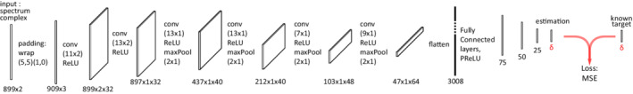
SPAWNN‐Quantification (SPAWNN‐Q) model architecture for metabolite concentration and parameter estimation. The convolutional neural network takes the spectrum as an input layer and performs six successive steps of convolution, ReLU activation, and pooling. Then, the five final steps are fully connected layers with PReLU activation. $\delta$ is equal to 20 for the parameters, and 14 for the metabolite concentration estimations.

The third network was a U‐Net model, as shown in Figure 3. The network was able to estimate the input spectrum's baseline, returning an array of the same size (899 complex points). The U‐Net was trained on 50 epochs with 500 spectra per mini‐batch. There were about $4·10^5$ parameters to train, with the training time taking around 6 h.

FIGURE 3.

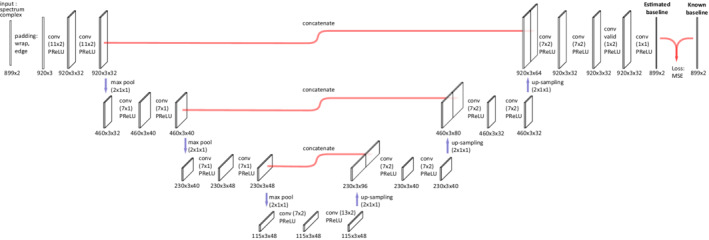
SPAWNN‐Baseline (SPAWNN‐Bl) model architecture for baseline estimation. The U‐Net takes the spectrum as an input layer and performs three down‐sampling steps with convolution and PReLU activation. Then, it performs three up‐scaling steps with convolution and PReLU activation. At each up‐scaling, the new layer is concatenated with the corresponding down‐sampling layer. The output is the estimation of the baseline and has the same dimension as the input.

3.3. LCModel

As reference for comparison, we have analyzed all ${}^{31}$P‐spectra using LCModel (Version 6.3‐1L). ⁴² The basis spectra were simulated using the GAMMA software library ³⁹ using the same physical model as for the simulated data for SPAWNN. The metabolites included in the basis were the 12 metabolites described above. Since phosphorus spectra were centered on the PCr peak at 0ppm, the reference peak was set at 15 ppm (PPMK = $-15$) for generating the basis set. The basis was created using a fixed linewidth of 5 Hz, with the LCModel parameters: DEEXT2 = 15 and DESDT2 = 10. For LCModel fitting, Pi and $\gamma$‐ATP were chosen as reference metabolites, resulting in the following parameters: CHUSE1 = 'Pi','gATP' and PPMREF(1,2) = 5. We set SDDEGP = 50 and SDDEGZ = 50 to enable LCModel to find the correct zero‐ and first‐order phases. The other parameters used were the same as those reported by Deelchand et al. ¹⁷

3.4. Magnetic resonance spectroscopy protocol

In vivo measurements were performed on a clinical Prisma‐fit 3T MRI scanner (Siemens Healthineers, Erlangen, Germany) equipped with multinuclear capabilities. Data were obtained from 10 healthy volunteers. Written informed consent was given by all the volunteers before participation and the study protocol was approved by the institutional ethics committee. No decoupling was applied during the phosphorus acquisition. Anatomical reference ${}^1$H images were obtained with T1‐weighted MP‐RAGE acquisition. The volunteers were scanned using a dual‐tuned ${}^1$H and ${}^{31}$P head coil (Clinical MR solutions, Brookfield, Wi.)

The unlocalized FID sequence consisted of a rectangular excitation pulse of 0.25 ms with a flip angle of $45^{\circ }$. The repetition time (TR) was set at 1500 ms, and the echo time (TE) was 0.35 ms with 32 averages. The bandwidth was 4000 Hz for 2048 sampling points. The acquisition took about 1 min. For three volunteers out of 10, another unlocalized FID was obtained using the same parameters, yet with 600 averages.

The 3D ${}^{31}$P‐MRSI was acquired on the whole brain with a $10\times 10\times 10$ matrix. The FOV dimension was 250 mm isotropic for a nominal spatial resolution of 25 mm isotropic. The sequence consisted of a rectangular excitation pulse of 0.25 ms with a flip angle of $45^{\circ }$. The repetition time (TR) was set at 1500 ms, and the echo time (TE) was 0.5 ms with 24 weighted averages. ⁴³ The bandwidth was 4000 Hz for 2048 sampling points. The acquisition took 37 min.

3.5. Spectrum processing

The in vivo FID data were extracted from the MRI raw data format. Averages and Fourier transforms were calculated using a Python script (Python Software Foundation, version 3.6.9), and the data were converted to Hierarchical Data Format (HDF5). No preprocessing was applied to the spectra prior to analysis.

3.6. Data analysis and statistic

The results estimated on the simulated dataset were analyzed using the coefficient of determination $R^2$. ⁴⁴ To compute the variability of the coefficient of determination, bootstrap statistics was performed on the data. ⁴⁵ The bootstrapping was performed by selecting randomly spectrum subsets with replacement and repeated computation of $R^2$ on these subsets. This evaluation was repeated 2000 times in order to compute the probability distribution of $R^2$.

Concerning volunteer data, no reference measurement was available to correct for variation of B1 and signal intensity, allowing absolute concentration estimation. Both methods, LCModel and SPAWNN, returned normalized concentration values that were within a constant, yet unknown, factor of the actual concentration value. The results were presented and analyzed as metabolite concentration ratios, since the ratio of two metabolites is independent of the scaling factor. ⁴⁶

The computational analysis was performed using Python.

4. RESULTS

Results of simulated data are shown in Figure 4. An example of a simulated spectrum with three decreasing SNR${}_{\text{mean}}$ (no noise added, 4, 2) is presented in panel (A). For illustration purposes, the simulated spectra shown in the figure do not contain baselines, phase or frequency shifts, and significant linewidth. Panel (B) illustrates the performance of SPAWNN and LCModel with the coefficient of determination $R^2$ and bootstrapping. The performance was assessed on another test set of $10^4$ spectra that were independent of the training dataset and never evaluated by the model before. The bootstrap statistics was computed using random spectra subset selection with replacement and repetition of the analysis 2000 times. The results showed similar to slightly better performance of SPAWNN compared with LCModel for the quantifying Pi, ATPs, PCr, PE, PCh, and GPE, with similar or higher $R^2$ values and smaller variance. Since LCModel displayed strong pairwise correlations between NAD+ and NADH, the total NAD (tNAD) concentration was computed for both methods for comparison purposes. The performance of SPAWNN in quantifying tNAD ($R^2=0.813[\pm 0.005]$) was comparable to that of other metabolites, whereas the results of LCModel were less accurate ($R^2=0.771[\pm 0.006]$). GPC concentration was better estimated with SPAWNN ($R^2=0.916[\pm 0.002]$) than LCModel ($R^2=0.862[\pm 0.005]$). Regarding MP estimation, both SPWANN ($R^2=0.770[\pm 0.004]$) and LCModel ($R^2=0.787[\pm 0.008]$) exhibited a low performance compared with all other metabolites, regardless of SNR bins (Figure 4C). Figure 4C shows the SPAWNN's coefficient of determination $R^2$ for each metabolite concentration estimation as a function of SNR range. The evaluation was performed on the simulated test dataset of $10^4$ spectra, separated in SNR bins with increment of 1. The coefficient of determination $R^2$ was computed on the entire test dataset between the model evaluation concentration and the ground truth. For all the metabolites, the value of the coefficient of determination decreased with SNR. Most metabolites had an $R^2$ value greater than 0.8 for all SNR bins. SPAWNN‐Bl evaluation of the test set baseline yielded a coefficient of determination of $R^2=0.97$ calculated between the pairwise correlation of the true baseline and the estimated baseline.

FIGURE 4.

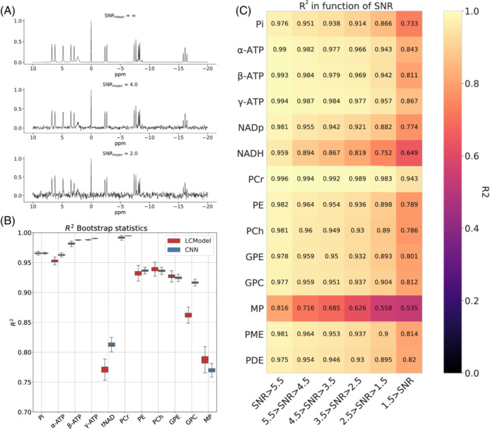
Results on simulated data. (A) Examples of SNR${}_{\text{mean}}$ for a simulated spectrum with no noise (top), SNR${}_{\text{mean}}$ of 4 (middle), and SNR${}_{\text{mean}}$ of 2 (bottom). (B) Comparison of the coefficient of determination $R^2$ with bootstrapping between SPAWNN and LCModel for each metabolite. A new dataset of $10^4$ spectra was created to compare the two methods. (C) SPAWNN's coefficient of determination $R^2$ for each metabolite concentration estimation as a function of the SNR${}_{\text{mean}}$ range.

Analyzed ${}^{31}$P‐MRSI in vivo data are shown in Figure 5 for SPAWNN (left) and LCModel (right). The data displayed are the sum of 8 voxels from the occipital cortex of one of the volunteers. The top plots are the spectra with either the reconstruction or the fit from each model. The middle plots are the residuals and the bottom plots show the signals for each metabolite separately. For SPAWNN, reconstruction of a spectrum was performed by using the estimated baseline, parameters, and concentration values, and by recreating the spectrum after Fourier transform of equation (2). The reconstructed spectrum is shown in red overlapping the in vivo data.

FIGURE 5.

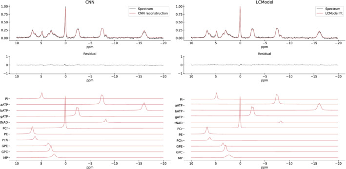
Comparison of in vivo ${}^{31}$P‐MRSI spectrum (TR = 1.5 s, TE = 0.5 ms, sum of 8 voxels with 24 weighted averages each) evaluated and reconstructed with SPAWNN (left) and fitted with LCModel (right). The figure displays SPAWNN reconstruction and the LCModel fit (top), the residuals (middle), and the contribution of each metabolite (bottom). No correction was applied before analysis.

Comparative analysis of the metabolite concentration ratio between LCModel and SPAWNN is displayed in Figure 6. The results were derived from the sum of 8 MRSI voxels located in the occipital region for each of the 10 volunteers. The mean value of $\alpha$‐ATP, $\beta$‐ATP, and $\gamma$‐ATP was computed and reported as ATP. The concentration of PCr was used as denominator for the ratios. Figure 6A shows a plot of the metabolite concentration ratio estimated by SPAWNN and LCModel, with a line connecting the data of the same subject. Figure 6B shows a Bland–Altman plot of the data from Figure 6C, with the difference between the SPAWNN and LCModel estimations versus the average of the two values. The mean difference between the two methods is $4.0·10^{-3}$, and the limits of agreements ($\pm 1.96\sigma$) are $+0.139$ and $-0.131$. The Bland–Altman plot shows few outliers, but no systematic bias. Relative differences and relative standard deviations are presented in Table 1. A statistical $t$‐test with Bonferroni correction was performed, and the $p$‐values are reported in the table as well. The Bonferroni correction took into account the repeated $t$‐tests (10 metabolites) and reduced the threshold for rejecting the null hypothesis to $\alpha =0.0056$. The metabolite ratios showed relative differences lower than 10% for most of the ratios, except for tNAD/PCr and MP/PCr. All metabolite ratios had a relative standard deviation higher than the relative differences, with none found to be significant.

FIGURE 6.

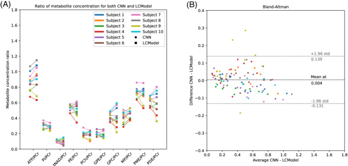
Results on ${}^{31}$P‐MRSI data, with the sum on 8 voxels. (A) Comparison of metabolite concentration ratios for the 10 volunteers with SPAWNN (circles) and LCModel (squares). ATP concentration is computed by averaging the concentration of the three resonances. (B) Bland–Altman plot of the difference between estimated values by SPAWNN and LCModel versus the average of the estimated values across all metabolite ratios and subjects.

TABLE 1.

Statistics of the comparison of the metabolic concentration ratio for the 10 volunteers with SPAWNN and LCModel from Figure 6

Metabolite ratio	Relative difference (%)	Relative standard deviation (%)	$p$‐value (uncorrected)
ATP/PCr	$-$4.69	6.93	0.073
Pi/PCr	7.37	7.68	0.018
tNAD/PCr	14.8	31.1	0.19
PE/PCr	3.0	13.6	0.53
PCh/PCr	2.16	15.5	0.68
GPE/PCr	8.36	11.4	0.055
GPC/PCr	1.63	11.3	0.83
MP/PCr	$-$10.4	15.5	0.075
PME/PCr	3.0	9.4	0.36
PDE/PCr	3.9	17.6	0.52

Note: Statistical $t$‐test was performed with Bonferroni correction for multiple comparisons resulting in a lower threshold for rejecting the null hypothesis to $\alpha =0.0056$. No difference in metabolite ratios was found to be significant.

Figure 7 illustrates the quantification performance of SPAWNN and LCModel with respect to noise. The data used were unlocalized FIDs with 600 averages acquired on three volunteers. The 600 spectra acquired were randomly selected retrospectively and averaged in groups ranging from 1 to 600 spectra. We considered the reference values to be the values estimated with 600 averages. The convergence was then defined as the difference between the mean value of the estimations and the reference value, with precision representing the standard deviation of the reference value. Figure 7 presents the results for the $\gamma$‐ATP, PCr, PE, PCh, GPC, and GPE. The two spikes in Subject #3 originate from an LCModel fatal error where the model failed to converge.

FIGURE 7.

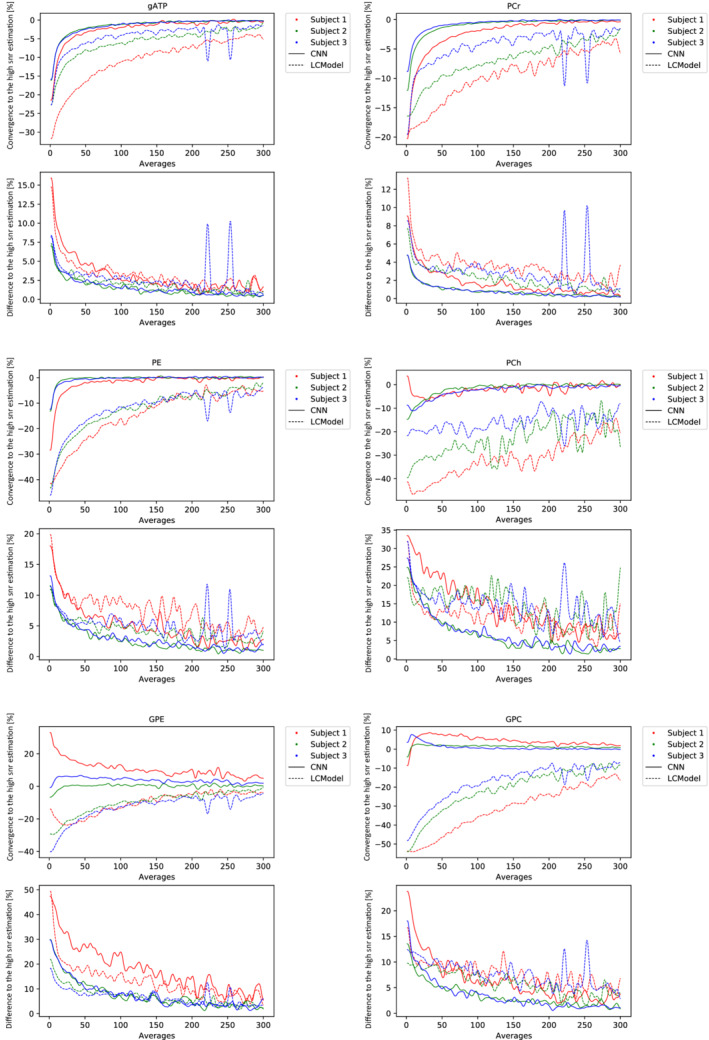
Results from unlocalized FID data of the occipital lobe. Comparison of metabolite concentration estimation by SPAWNN and LCModel. The reference value is the estimate obtained with the average of the full acquisition (600 spectra). The plots show the convergence and the difference in estimation of each model with respect to the highest SNR estimate.

Analysis of single voxels from in vivo ${}^{31}$P‐MRSI with the two methods is shown in Figure 8. The SPAWNN spectrum reconstruction from two distinct brain voxels is displayed. The T1 MP‐RAGE ${}^1$H image is presented on the left; the grid shows the voxel locations in the sagittal view (top) and the corresponding axial slice (bottom) centered on the blue box location. The analysis of voxel A and B with SPAWNN and LCModel is shown on the right. Each spectrum is presented with either the reconstruction or the fit, with the residual underneath. The estimated SNR${}_{\text{mean}}$ for the spectra were 1.56 and 1.63, and the LCModel SNRs were 16 and 20 for voxels A and B, respectively.

FIGURE 8.

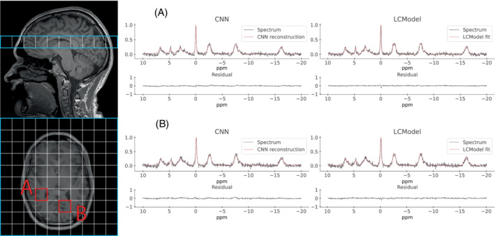
Examples of SPAWNN evaluation of a 3D ${}^{31}$P‐MRSI acquired on a human brain. The figure shows two spectra (TR = 1.5 s, TE = 0.5 ms, 24 weighted averages) arising from two brain regions. The T1 MP‐RAGE ${}^1$H MRI is displayed on the left, indicating the slice position and voxel locations. The voxel has a resolution of 25 mm isotropic. The spectra on the left represent the SPAWNN reconstruction with the measurement data, and the spectra on the right the LCModel fitting for voxels A and B.

5. DISCUSSION

This study demonstrated the ability of SPAWNN to evaluate, quantify, and reconstruct ${}^{31}$P‐MRS data. We focused on two network architectures specifically developed to fully identify spectral features of MRS data. SPAWNN‐Q, displayed in Figure 2, was used to extract the metabolite concentrations and spectral parameters. We used two separate networks running in parallel for efficiency and flexibility, which also allowed for a better control of the training phase during model development. However, a single LeNet for both concentration and parameters estimation was tested and yielded similar results. SPAWNN‐Q parameter network can be applied to MRSI data for phases and frequency shift correction in order to sum individual spectra before complete quantification. SPAWNN‐Bl (Figure 3) was used for spectral baseline estimation.

Our synthetic dataset was simulated by summing independent metabolite signals. However, ATP was simulated as three independent resonances for $\gamma$‐, $\alpha$‐, and $\beta$‐ATP, thereby rendering the network more flexible in estimating concentration as well as chemical shift. The reason for this choice was that other metabolites, such as adenosine diphosphate (ADP), may overlap with $\gamma$‐ and $\alpha$‐ATP and influence the estimated concentration. In addition, three ATP resonances were shown to exhibit different chemical shifts with varying concentrations of Mg${}^{2+}$. ⁴⁷ However, our physical model assumed the same linewidth for the three ATP resonances because of their identical T2 relaxation times. SPAWNN results demonstrated a high performance on simulated datasets as well as on in vivo data (Figures 4 and 6). This indicates that our simulation model (equation (2)) is a good emulation of the physical NMR signal and faithfully represents the measured spectra using excite–acquire sequences. The SPAWNN evaluations presented in Figures 5 and 8 show the reconstruction of the spectra and illustrate the ability of SPAWNN to provide a good estimation of the spectral parameters, concentrations, and baseline, as the reconstructions matched the spectra. Artificial intelligence (AI) approaches, such as CNN, perform accurately if the measured parameters are in the range of the training set. For specific applications, it might be possible to train the network with a smaller range of concentrations to possibly achieve better performance. One could imagine having a specialized model for each organ, with the concentration distribution centered on the values reported in the literature. However, training with a narrower parameter distribution could induce a bias in the analysis of specific conditions or pathologies that strongly affects the metabolism. Moreover, in a situation where data are acquired with parameters outside the training range (e.g., strong artifact), the results of the analysis should be discarded. The spectral reconstruction based on estimates is an important tool to visually validate whether the neural network estimate matches the in vivo spectrum, in which case the results should be discarded. In this study, we chose to train the networks over a very wide range of parameter values to avoid this limitation. This wide range does not compromise the quantification accuracy while avoiding bias.

On the simulated data, SPAWNN compared favorably to LCModel in terms of precision. The coefficient of determination $R^2$ per metabolites, as a whole, was similar for both approaches (Figure 4B). Of the 11 metabolites, only three significantly differed between the two methods. SPAWNN performed better for tNAD and GPC, while LCModel showed better performance on MP. NAD+ and NADH can be accurately estimated with LCModel at 7T, ⁴⁸ due to the higher signal and greater chemical shift dispersion. By contrast, at 3T without proton decoupling, the distinction between NAD+ and NADH is more difficult, as illustrated by the results where tNAD was estimated with the least accuracy. MPs were also estimated with low accuracy by both SPAWNN and LCModel. This is due to the larger peak width that makes the distinction between the baseline and noise difficult. Figure 4B shows that with bootstrap statistics, the standard deviation of the coefficient of determination of the LCModel was larger than that of SPAWNN for all metabolites. In addition, SPAWNN estimates remained accurate ($R^2>0.8$) for most metabolites at a very low SNR (Figure 4C), highlighting the robustness of the method.

In vivo data (Figures 5 and 8) showed that SPAWNN can estimate the spectral parameters with good accuracy, since the reconstruction of the spectra based on these estimates closely matched the measured data. An example of analysis with both methods for a volunteer is presented in Figure 5. The data were obtained by summing 8 neighbor voxels in the occipital region. By contrast, an analysis with both methods for singles voxels of the volunteer data is shown in Figure 8. The individual signals of each metabolite as estimated by SPAWNN and LCModel are displayed in Figures 5 and 8. The two methods showed consistent signal for each metabolite. The residuals are low with both approaches but nevertheless slightly higher with SPAWNN. This is explained by the fact that LCModel is a fitting algorithm while SPAWNN does not aim at minimizing the residuals. Figure 6 presents the concentration ratio values of the metabolites obtained on 8 averaged voxels from the occipital region of each subject. The results are in very good agreement with the values reported using PCr as internal reference. ⁴⁶ , ⁴⁹ , ⁵⁰ The Bland–Altman plot shows that the mean difference of the two methods was much smaller than the standard deviation and demonstrates the absence of bias. The outlier points in Subject #9 could be explained by poor B0 homogeneity during the acquisition. By contrast, Subject #7 was the one with the best B0 homogeneity and showed close estimation with both methods. Table 1 reveals that all relative standard deviations were greater than the relative differences, indicating that inter‐subject variation was greater than between‐method variation.

Figure 7 shows the convergence toward the estimated value at high SNR by SPAWNN and LCModel. The data originate from unlocalized FID with 600 averages acquired from three volunteers. Unlocalized FID was used instead of MRSI in order to get optimum SNR with reasonable acquisition duration considering 600 averages. The plots aim to present the convergence of both models toward the reference value estimated at the highest SNR, corresponding to the spectra obtained with 600 averages. For high‐signal metabolites, such as PCr and ATPs, both models displayed similar speed of convergence. For lower‐signal metabolites, such as PCh and GPC, the estimation with LCModel differed by more than 10% from the high SNR value even with high numbers of averages. SPAWNN showed faster asymptotic convergence toward the concentration reference. Both SPAWNN and LCModel demonstrated similar precisions, with more variation across subjects than across methods. Spectra from Subject #1 had more noise and half lower SNR compared with the other two subjects, which can be due to worst shimming. The discontinuities observed in Subject #2 are attributable to LCModel failure to converge (“fatal errors”) and were considered as outliers. Over all the metabolites, SPAWNN displayed more consistency and stability, especially at low SNR. This result suggests that the SPAWNN approach is more robust at low SNR than LCModel, thus implying a fewer number of averages to match the results of traditional fitting methods. This could translate into shorter acquisition time in a clinical setting or higher reconstruction resolution for MRSI.

SPAWNN training time was 4 and 6 h for the two submodels. Nevertheless, once the weights were computed, spectral analysis with SPAWNN was almost instantaneous. Indeed, the evaluation of $10^5$ spectra required approximately 5 min. This could be useful in the prospect of applying the method to 3D metabolite mapping, which requires the analysis of the full dataset. As illustrated in Figure 8, the $10^3$ voxels of the dataset were analyzed in a few minutes, whereas the same analysis performed by LCModel lasted almost 1 h. Faster computing time is a clear advantage for clinical applications where a fast online processing is highly desired.

Our study results compared with those of previously published works that used neural network approaches to analyze MRS. ¹⁴ , ²³ , ²⁴ Das et al. ¹⁴ presented a method using random forest machine learning, while Hatami et al. ²³ used a DL CNN model for quantification. Compared with both methods, the physical model proposed here for generating the simulated training set includes a larger number of parameters, which should result in a more complete variety of spectra, as well as artifacts and distortions, as observed in vivo. The approach proposed by Lee et al. ²⁴ aimed to learn the reconstruction of the spectral real part, while ours aimed to learn the metabolite concentration and parameters directly, without optimized reconstruction. Other studies used a different approach to applying AI to NMR, such as the one conducted by Da‐Wei et al. ⁵¹ who used a neural network approach to perform deconvolution on overlapping peaks.

The analysis was performed without measuring a reference signal, with therefore no possibility of absolute quantification, and LCModel was used as a fair reference for comparison of metabolite ratios. In a possible perspective, both models could be compared for absolute quantification with the measurement of an in vitro reference with a known concentration. The influence of the training parameter ranges over SPAWNN robustness and stability remains to be established. As mentioned above, narrow specific parameter ranges might improve accuracy but SPAWNN results would be unreliable for spectral parameters falling outside the training range. Possible improvements of SPAWNN can be explored: the physical model could notably be improved by taking into account more distortions, such as eddy current effects. Future developments also include implementing SPAWNN for metabolite mapping and determining a confidence interval for the estimated values.

In conclusion, we presented a DL method of evaluation, quantification, and baseline estimation for ${}^{31}$P‐MRS, combined with a reconstruction pipeline for spectral reconstruction. The proposed SPAWNN method had a high accuracy and robustness overall, especially at low SNR, thereby allowing higher resolution reconstruction in MRSI schemes. Our proposed approach had an extremely fast computation time that offers the ability to analyze large ${}^{31}$P‐MRSI datasets almost instantaneously, which is a significant advantage for possible applications in a clinical setting.

Songeon J, Courvoisier S, Xin L, et al. In vivo magnetic resonance ${}^{31}$P‐Spectral Analysis With Neural Networks: 31P‐SPAWNN. Magn Reson Med. 2023;89:40‐53. doi: 10.1002/mrm.29446

DATA AVAILABILITY STATEMENT

The source code for the proposed 31P‐SPAWNN model can be downloaded from this link: https://gitlab.unige.ch/Julien.Songeon/31P‐SPAWNN.

REFERENCES

- 1. Reto B, Dieter M, Ernst M, Peter B. Assessment of absolute metabolite concentrations in human tissue by 31P MRS in vivo part II: muscle, liver, kidney. Magn Reson Med. 1994;32:453‐458. [DOI] [PubMed] [Google Scholar]
- 2. Chmelik M, Schmid A, Gruber S, et al. Three‐dimensional high‐resolution magnetic resonance spectroscopic imaging for absolute quantification of 31P metabolites in human liver. Magn Reson Med. 2008;60:796‐802. [DOI] [PubMed] [Google Scholar]
- 3. Webb Graham A, ed. Methods and applications of phosphorus NMR spectroscopy in vivo. Annual Reports on NMR Spectroscopy. Vol 75. Academic Press; 2012. [Google Scholar]
- 4. Jong‐Hee H, Soo CC. Use of in vivo magnetic resonance spectroscopy for studying metabolic diseases. Exp Mol Med. 2015;47:e139. [DOI] [PMC free article] [PubMed] [Google Scholar]
- 5. Rudin M, ed. In‐Vivo Magnetic Resonance Spectroscopy III: In‐Vivo MR Spectroscopy: Potential and Limitations. Springer Berlin Heidelberg; 1992. [Google Scholar]
- 6. Boulangé CL. Nuclear magnetic resonance spectroscopy‐applicable elements| Phosphorus‐31. Reference Module in Chemistry, Molecular Sciences and Chemical Engineering. Elsevier; 2017. [Google Scholar]
- 7. Maudsley AA, Hilal SK, Perman WH, Simon HE. Spatially resolved high resolution spectroscopy by “four‐dimensional” NMR. J Magn Reson. 1983;51:147‐152. [Google Scholar]
- 8. Thulborn KR, Atkinson IC. Quantitative metabolic magnetic resonance imaging of sodium, oxygen, phosphorus and potassium in the human brain. Magnetic Resonance Spectroscopy. Elsevier; 2014:291‐311. [Google Scholar]
- 9. Hongyan Q, Xiaoliang Z, Zhu X‐H, Fei D, Wei C. In vivo 31P MRS of human brain at high/ultrahigh fields: a quantitative comparison of NMR detection sensitivity and spectral resolution between 4T and 7T. Magn Reson Imaging. 2006;24:1281‐1286. [DOI] [PMC free article] [PubMed] [Google Scholar]
- 10. Ladislav V, Marek C, Martin M, et al. Dynamic31P‐MRSI using spiral spectroscopic imaging can map mitochondrial capacity in muscles of the human calf during plantar flexion exercise at 7T. NMR Biomed. 2016;29:1825‐1834. [DOI] [PMC free article] [PubMed] [Google Scholar]
- 11. Goldenberg S, Larry NG, Salcudean Septimiu E. A new era: artificial intelligence and machine learning in prostate cancer. Nat Rev Urol. 2019;16:391‐403. [DOI] [PubMed] [Google Scholar]
- 12. Scott K. Feature learning and deep learning architecture survey. Computer Vision Metrics: Textbook Edition. Springer International Publishing; 2016:375‐514. [Google Scholar]
- 13. Jinchao L, Margarita O, Lorna A, Michael F, Solomon Christopher J, Gibson Stuart J. Deep convolutional neural networks for Raman spectrum recognition: a unified solution. Analyst. 2017;142:4067‐4074. [DOI] [PubMed] [Google Scholar]
- 14. Dhritiman D, Eduardo C, Schulte Rolf F, Menze Bjoern H. Quantification of metabolites in magnetic resonance spectroscopic imaging using machine learning. Medical Image Computing and Computer Assisted Intervention ‐ MICCAI 2017. Springer International Publishing; 2017:462‐470. [Google Scholar]
- 15. Provencher S. Automatic quantitation of localized in vivo 1H spectra with LCModel. NMR Biomed. 2001;14:260‐264. [DOI] [PubMed] [Google Scholar]
- 16. Pierre‐Gilles H, Gülin Ö, Stephen P, Rolf G. Toward dynamic isotopomer analysis in the rat brain in vivo: automatic quantitation of 13C NMR spectra using LCModel. NMR Biomed. 2003;16:400‐412. [DOI] [PubMed] [Google Scholar]
- 17. Kumar DD, Tra‐My N, Xiao‐Hong Z, Fanny M, Pierre‐Gilles H. Quantification of in vivo 31P NMR brain spectra using LCModel. NMR Biomed. 2015;28:633‐641. [DOI] [PMC free article] [PubMed] [Google Scholar]
- 18. Selvikvåg LA, Arvid L. An overview of deep learning in medical imaging focusing on MRI. Z Med Phys. 2019;29:102‐127. [DOI] [PubMed] [Google Scholar]
- 19. Singh SP, Lipo W, Sukrit G, Haveesh G, Parasuraman P, Balázs G. 3D deep learning on medical images: a review arXiv e‐prints, arXiv:2004.00218.
- 20. Marina C, Simone S, Francesco S. Trimboli Rubina Manuela. Artificial intelligence for breast MRI in 2008–2018: a systematic mapping review. Am J Roentgenol. 2019;212:280‐292. [DOI] [PubMed] [Google Scholar]
- 21. Aurélien B, Niccolo F, Botnar René M, Claudia P. From compressed‐sensing to artificial intelligence‐based cardiac MRI reconstruction. Front Cardiovascular Med. 2020;7:17. [DOI] [PMC free article] [PubMed] [Google Scholar]
- 22. Fan L, Yudu L, Guo R, Bryan C, Zhi‐Pei L. Ultrafast magnetic resonance spectroscopic imaging using SPICE with learned subspaces. Magn Reson Med. 2019;83:377‐390. [DOI] [PMC free article] [PubMed] [Google Scholar]
- 23. Nima H, Michaël S, Hélène R. Magnetic resonance spectroscopy quantification using deep learning. Medical Image Computing and Computer Assisted Intervention – MICCAI 2018. Springer International Publishing; 2018:467‐475. [Google Scholar]
- 24. Hun LH, Hyeonjin K. Deep learning‐based target metabolite isolation and big data‐driven measurement uncertainty estimation in proton magnetic resonance spectroscopy of the brain. Magn Reson Med. 2020;84:1689‐1706. [DOI] [PubMed] [Google Scholar]
- 25. Fan L, Yahang L, Xi P. Constrained magnetic resonance spectroscopic imaging by learning nonlinear low‐dimensional models. IEEE Trans Med Imaging. 2020;39:545‐555. [DOI] [PubMed] [Google Scholar]
- 26. Courvoisier S, Klauser A, Lazeyras F. High‐resolution magnetic resonance spectroscopic imaging quantification by convolutional neural network. Proceedings of the 2019 Annual Meeting of the International Society for Magnetic Resonance in Medicine (ISMRM). 2019; 27: 0519.
- 27. Varanavasi G, Karl Y, Maudsley Andrew A. Proton NMR chemical shifts and coupling constants for brain metabolites. NMR Biomed. 2000;13:129‐153. [DOI] [PubMed] [Google Scholar]
- 28. Ernst RR, Bodenhausen G, Wokaun A. Principles of Nuclear Magnetic Resonance in One and Two Dimensions. Vol 7. Wiley; 1988:158‐165. [Google Scholar]
- 29. Lecun Y, Bottou L, Bengio Y, Haffner P. Gradient‐based learning applied to document recognition. Proc IEEE. 1998;86:2278‐2324. [Google Scholar]
- 30. Olaf R, Philipp F, Thomas B. U‐net: convolutional networks for biomedical image segmentation. LNCS. 2015;9351:234‐241. [Google Scholar]
- 31. Bhargab BM, Dinthisrang D, Khwairakpam A, Debdatta K. Handwritten character recognition from images using CNN‐ECOC. Procedia Comput Sci. 2020;167:2403‐2409. [Google Scholar]
- 32. Shengnan C, Heng Z, Yang X, et al. Raman spectroscopy reveals abnormal changes in the urine composition of prostate cancer: an application of an intelligent diagnostic model with a deep learning algorithm. Adv Intel Syst. 2021;3:2000090. [Google Scholar]
- 33. Dicheng C, Wang Z, Guo D, Vladislav O, Xiaobo Q. Review and prospect: deep learning in nuclear magnetic resonance spectroscopy. arXiv e‐prints, arXiv:2001.04813. [DOI] [PubMed]
- 34.Albawi S., Mohammed T.A. and Al‐Zawi S. Understanding of a convolutional neural network. Proceedings of the 2017 International Conference on Engineering and Technology (ICET), 2017, pp. 1‐6.
- 35. Zhang Z, Liu Q, Wang Y. Road extraction by deep residual U‐net. IEEE Geosci Remote Sens Lett. 2018;15:749‐753. [Google Scholar]
- 36. Zohaib I, Dan N, Albert TM, Steve J. Deep learning can accelerate and quantify simulated localized correlated spectroscopy. Sci Rep. 2021;11:8727. [DOI] [PMC free article] [PubMed] [Google Scholar]
- 37. Kyathanahally SP, Döring A, Kreis R. Deep learning approaches for detection and removal of ghosting artifacts in MR spectroscopy. Magn Reson Med. 2018;80:851‐863. [DOI] [PubMed] [Google Scholar]
- 38. Zahangir AM, Chris Y, Mahmudul H, Taha Tarek M, Asari Vijayan K. Recurrent residual U‐net for medical image segmentation. J Med Imag. 2019;6:1. [DOI] [PMC free article] [PubMed] [Google Scholar]
- 39. Smith SA, Levante TO, Meier BH, Ernst RR. Computer simulations in magnetic resonance. An object‐oriented programming approach. J Magn Reson A. 1994;106:75‐105. [Google Scholar]
- 40. Kingma DP, Jimmy B. ADAM: a method for stochastic optimizationarXiv e‐prints, arXiv:1412.6980. 2014.
- 41. Ida T, Ando M, Toraya H. Extended pseudo‐Voigt function for approximating the Voigt profile. J Appl Crystallogr. 2000;33:1311‐1316. [Google Scholar]
- 42. Provencher Stephen W. Estimation of metabolite concentrations from localized in‐vivo proton NMR spectra. Magn Reson Med. 1993;30:672‐679. [DOI] [PubMed] [Google Scholar]
- 43. Rolf P, Markus K. Accurate phosphorus metabolite images of the human heart by 3D acquisition‐weighted CSI. Magn Reson Med. 2001;45:817‐826. [DOI] [PubMed] [Google Scholar]
- 44. Davide C, Warrens Matthijs J, Giuseppe J. The coefficient of determination R‐squared is more informative than SMAPE, MAE, MAPE, MSE and RMSE in regression analysis evaluation. Pee rJ Comput Sci. 2021;7:e623. [DOI] [PMC free article] [PubMed] [Google Scholar]
- 45. Efron B. Bootstrap methods: another look at the Jackknife. Anna Stat. 1979;7:1‐26. [Google Scholar]
- 46. Andreas R, Ruth S, Stephanie M, et al. Energy metabolis measured by 31P magnetic resonance spectroscopy in the healthy human brain. J Neuroradiol. 2022. [DOI] [PubMed] [Google Scholar]
- 47. Gout E, Rebeille F, Douce R, Bligny R. Interplay of mg, ADP, and ATP in the cytosol and mitochondria: unravelling the role of mg in cell respiration. Proc Natl Acad Sci U S A. 2014;111:E4560‐E4567. [DOI] [PMC free article] [PubMed] [Google Scholar]
- 48. Xin L, Ipek Ö, Beaumont M, et al. Nutritional ketosis increases NAD+/NADH ratio in healthy human brain: an in vivo study by 31P‐MRS. Front Nutr. 2018;5:62. [DOI] [PMC free article] [PubMed] [Google Scholar]
- 49. Jensen J, Eric DDJ, Menon Ravi S, Williamson Peter C. In vivo brain 31P‐MRS: measuring the phospholipid resonances at 4 tesla from small voxels. NMR Biomed. 2002;15:338‐347. [DOI] [PubMed] [Google Scholar]
- 50. Jimin R, Dean SA. Malloy Craig R. 31P‐MRS of healthy human brain: ATP synthesis, metabolite concentrations, pH, and T1 relaxation times. NMR Biomed. 2015;28:1455‐1462. [DOI] [PMC free article] [PubMed] [Google Scholar]
- 51. Da‐Wei L, Hansen Alexandar L, Chunhua Y, Lei B‐L, Rafael B. DEEP picker is a DEEP neural network for accurate deconvolution of complex two‐dimensional NMR spectra. Nat Commun. 2021;12:5229. [DOI] [PMC free article] [PubMed] [Google Scholar]
Associated Data
This section collects any data citations, data availability statements, or supplementary materials included in this article.