Optimal Transport Features for Morphometric Population Analysis

Abstract

Brain pathologies often manifest as partial or complete loss of tissue. The goal of many neuroimaging studies is to capture the location and amount of tissue changes with respect to a clinical variable of interest, such as disease progression. Morphometric analysis approaches capture local differences in the distribution of tissue or other quantities of interest in relation to a clinical variable. We propose to augment morphometric analysis with an additional feature extraction step based on unbalanced optimal transport. The optimal transport feature extraction step increases statistical power for pathologies that cause spatially dispersed tissue loss, minimizes sensitivity to shifts due to spatial misalignment or differences in brain topology, and separates changes due to volume differences from changes due to tissue location. We demonstrate the proposed optimal transport feature extraction step in the context of a volumetric morphometric analysis of the OASIS-1 study for Alzheimer’s disease. The results demonstrate that the proposed approach can identify tissue changes and differences that are not otherwise measurable.

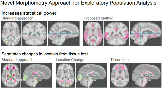
Graphical Abstract

1. Introduction

Neurological diseases and disorders produce subtle and varied changes in brain anatomy that can be diffuse in nature and affect tissue volume as well as the relative position and shape of brain anatomy. Detecting and quantifying these changes are the primary goals of image-based morphometric population analysis studies. Popular methods include cortical-surface-based analysis (Dale et al., 1999) or volumetric methods such as voxel-based morphometry (VBM) (Ashburner and Friston, 2000) or tensor-based morphometry (TBM) (Ashburner, 2007; Hua et al., 2008) and its variants. Morphometric methods have been applied to a wide variety of neuroimaging studies ranging from Alzheimer’s disease (Hua et al., 2008) to schizophrenia (Scarpazza and De Simone, 2016).

The standard morphometric analysis pipeline for both surface and volumetric analysis is based on three main steps: (1) spatial alignment, (2) extraction of the quantity of interest, and (3) statistical analysis on the spatial domain. While the specifics vary greatly for different methods, the main steps remain the same and the statistical analysis is based on the analysis of quantities defined at discrete locations on a spatial domain: per voxel in volumetric approaches and per vertex for surface based approaches. We propose adding optimal transport features (OTF) as an additional feature extraction step that precedes the statistical analysis. This can increase statistical power for the discovery of spatially diffuse effects, it can reduce sensitivity to spatial misalignments, and it can separate changes in quantity from changes due to shifts in tissue location.

The feature extraction step is based on unbalanced optimal transport and was first introduced in the context of VBM as unbalanced optimal transport morphometry (UTM) (Gerber et al., 2018). We emphasize that this methodology can be used in settings other than the VBM analysis pipelines (e.g. surface-based) by adding the OTF step before the statistical analysis. This work uses volumetric-based approaches, in particular voxel- and tensor-based morphometric (VBM, TBM), to demonstrate the properties of OTF. Voxel-based analysis compares tissue amounts at each voxel and captures spatially localized changes in brain anatomy. The distribution at a particular voxel is not only dependent on the amount of tissue but also on anatomical shape, as the gyri and sulci typically do not perfectly align after spatial normalization due to topological differences. Even with a hypothetical perfect alignment, tissue loss can be diffuse and spread out over a large region, affecting different locations within a region per individual. The local analysis in VBM/TBM has difficulty in detecting such regionally or diffusely occurring individual changes. Figure 1 illustrates how OTF improve sensitivity to diffuse tissue loss on a TBM analysis of gray matter tissue volume in correlation with clinical dementia ratings.

Fig. 1.

Tensor-based morphometric analysis of gray matter tissue without and with the optimal transport feature extraction step. The pink color shows inverse correlation strength of gray matter between patients with mild dementia compared to normal aging controls for voxels with Bonferroni corrected p < 0.05. The optimal transport feature extraction improves the statistical power and shows regions of gray matter tissue loss associated with mild dementia that are not identified with a standard TBM analysis (more details of the analysis are in Section 5).

Optimal transport, as the name implies, solves the problem of transporting mass from a source probability measure μ to a target probability measure ν, such that the cost of moving mass from the source μ to the target ν is minimized. Unbalanced optimal transport (Guittet, 2002; Benamou, 2003) extends optimal transport to measures that do not need to have equal mass by adding a mechanism to add (or remove) mass to the optimization problem. The solution of the unbalanced optimal transport problem yields a transport plan, or coupling, that measures local mass allocation as well as transport cost, i.e., the movement of mass between source and target locations. These two measures explicitly separate changes in amount of tissue from differences in relative location of tissue due to variation in position and shape of individual anatomy. This results in two main improvements over the traditional voxel-based analysis approaches. First, the decoupling of tissue allocation and tissue movement makes OTF less sensitive to shape variations and shifts in location of anatomy. Second, the explicit modeling of mass allocation improves statistical power when tissue loss (or gain) is spatially dispersed.

This paper extends the OTF approach (Gerber et al., 2018) by using a template (Section 3.1) and adding localized mass-balancing (Section 3.2). The use of a template avoids the computation of pairwise transport maps between all images and requires only transport maps from each image to the template image. The original OTF formulation enforces a global mass-balancing. This can mask regional effects of smaller magnitude if there are large variations in total mass in the population. We propose a mechanism to enforce mass-balancing at intermediate scales by adding a cost to allocating or removing mass. This localized mass-balancing approach provides a continuum between the VBM/TBM approach and the global mass equalization approach in the originally proposed OTF.

We provide a statistical analysis and evaluate the method using real-world data. The statistical analysis quantifies the increase in correlation strength for diffuse tissue loss (Section 4). A key finding of the statistical analysis is that OTF require a smaller sample size than VBM/TBM to detect differences and yields non-negligible correlations for even very small diffuse tissue loss differences between populations. We demonstrate the OTF analysis approach in the context of a VBM and TBM analysis on the OASIS-1 Dementia study data (Section 5). The OTF analysis of real world data supports the theoretical results from Section 4 and shows stronger correlations for diffuse pathology. The OTF results based on real-world data also demonstrate the capability to separate changes due to shape from tissue loss effects.

2. Related Work

VBM (Ashburner and Friston, 2000) uses a smoothed tissue mask to correlate each voxel with a clinical variable of interest. The first step of VBM is spatial alignment, but the alignment needs to be done at a global scale in order to preserve some of the local variation in tissue masks (Frackowiak, 2004, Chapter 7). TBM (Ashburner, 2007) modifies VBM by using the Jacobian determinant of a deformable spatial alignment, rather than using a smoothed tissue mask, at each voxel to correlate with a clinical variable of interest. The Jacobian determinant provides a measure of local volume changes in the spatial alignment, and this allows TBM to provide better results given better local spatial alignment. TBM mitigates some of the difficulties associated with choosing a spatial alignment in VBM. However, even with state of the art deformable registration, perfect alignment is typically not achieved, and the Jacobian determinant depends strongly on the amount of regularization of the deformable registration.

Deformation-based morphometry (DBM) (Ashburner et al., 1998) addresses the issue of detecting shape variations by comparing the parameters of non-linear deformations to a template. DBM typically requires segmentation of the anatomy of interest and the DBM results, typically shown as modes of variation of the anatomy, are more difficult to visualize and interpret.

The OTF analysis combines strengths of VBM/TBM and DBM methods. While the results are based on a voxel-wise analysis and are easily interpretable, the quantities compared stem from a global optimization problem that can detect global and regional shape variations and tissue loss effects. On the other hand, VBM, TBM, and DBM are driven by local image gradients, and voxel-wise measures ultimately lead to very similar results. The OTF method solves a global optimization problem based on the distribution of mass, and the allocation of mass is not driven solely by image gradients. With OTF, allocation of mass can be diffuse over a large region without the need for a smooth spatial normalization to distribute the image gradient driven warp over a larger region. TBM and DBM are not able to capture diffuse tissue loss consisting of small deteriorations at multiple locations if the tissue loss does not affect anatomical boundaries. VBM detects such loss but requires more data samples compared to OTF, as we show in Section 4.

VBM is known to be sensitive to the particulars of the spatial normalization (Bookstein, 2001; Davatzikos, 2004). OTF still depend on a spatial normalization to bring the participants into a common coordinate system such that distances between voxels across participants are meaningful. However, optimal transport is insensitive to small miss-alignments in the spatial normalization step; small shifts in mass locations incur only small transport costs.

There are several different formulations of optimal transport theory, with much recent interest in extending the formulations and algorithms to the unbalanced case. The fluid dynamic formulation of optimal transport, introduced by (Benamou and Brenier, 2000), was extended to the unbalanced case by (Liero et al., 2017; Chizat et al., 2018; Gangbo et al., 2019; Lee et al., 2021). When the measures are finitely supported, the optimal transport problem becomes equivalent to an assignment problem (Mérigot and Thibert, 2021), and unbalanced transport similarly becomes unbalanced assignment; The unbalanced assignment problem has its own history of algorithm development; a summary can be found in (Prakash et al., 2022). In this work, we present unbalanced transport as a linear program, and we frame this in our software as a minimum cost flow problem that we solve using the Network Simplex Method (Ahuja et al., 1993). Recent advances in the computation of optimal transport plans (Cuturi, 2013; Gerber and Maggioni, 2017) paved the way for a flurry of applications in machine learning and spurred interest in applications to medical image analysis. Gramfort et. al. (Gramfort et al., 2015) used optimal transport for improved averaging of neuroimaging data, Feydy et al. (Feydy et al., 2017) used unbalanced optimal transport as a similarity measure for diffeomorphic registration, and Kundu et. al. (Kundu et al., 2018) formulated a DBM approach, TrBM, which replaces non-linear warps by optimal transport plans.

3. Unbalanced Optimal Transport Morphometry

The OTF approach follows the standard voxel-wise morphometry pipeline with a few additions. The main difference is that the OTF analysis uses mass allocation images derived from the solution of unbalanced optimal transport between the participants and a template. The basic pipeline consists of spatial alignment, construction of a template image, computation of optimal transport features for each subject, and voxel-wise correlation of those features.

We introduce a template based approach instead of pairwise transport maps between all participants to construct allocation and transport cost images. The template-based approach (Section 3.1) reduces the computational burden and restricts mass allocation to the support of the template. Finally, we describe a modification of the unbalanced optimal transport linear program that allows for localized mass-balancing strategies (Section 3.2) and shows that OTF analysis forms a continuum between voxel-wise VBM/TBM and a global mass balancing approach.

3.1. Template Construction

For the template-based approach we considered three approaches to construct a template from a set of spatially aligned images X_i. A simple approach to construct a template is the voxel-wise mean, i.e. a Euclidean mean $E=\frac{1}{n}{\sum }_i{X}_i$. This leads to a template with a large number of non-zero voxels and increases the computation time of the optimal transport described in Section 3.2. To reduce the number of non-zero voxels we considered a sparse mean E_s = E ⊗ B_s, where ⊗ denotes a voxel-wise product of images, and where B_s is a binary image with

$$B_s(x)=\{\begin{array}{c}1,\text{if}{\sum }_i{1}_{>0}(X_i(x))\ge s\hfill \\ 0,\text{otherwise}.\hfill \end{array}\phantom{\}}$$ (1)

Here $1_{>0}$ is the indicator function that takes the value 1 on positive inputs and vanishes otherwise. In other words, E_s is the mean but only at voxels where more than s images have a positive value.

Finally, we consider the optimal transport barycenter:

$$E_o=\text{arg}\underset{Y}{\text{min}}\sum _{i}d(X_i,Y{)}^2$$ (2)

where d(X_i, Y) is the unbalanced optimal transport distance described in Section 3.3. There are several algorithms to compute the optimal transport barycenter (Anderes et al., 2016; Cuturi and Doucet, 2014). We use an approximate approach by iteratively updating the locations in Y depending on the optimal transport plans from each X_i.

In practice we did not see any differences in the results with different types of means and use the sparse Euclidean mean approach due to its computational efficiency.

3.2. Unbalanced Optimal Transport with Local Mass-Balancing

For two probability measures μ and ν on probability spaces X and Y respectively, a coupling of μ and ν is a measure π on X × Y such that the marginals of π are μ and ν. The coupling π defines a transport plan that captures how much mass π(x, y) is transported from x ∈ X to y ∈ Y. To define optimal transport, we need a cost function c(x, y) on X × Y, representing the work or cost of moving a unit of mass (tissue) from x to y. The cost is typically the Euclidean distance between the tissue locations but can be defined differently depending on the application domain, e.g. distance on the cortical surface for surface-based analysis. An optimal coupling π* minimizes this cost over all choices of couplings $C(\mu ,\nu )$ between μ and ν:

$${\pi }^{\ast }=\underset{\pi \in 𝒞(\mu ,\nu )}{\text{argmin}}{\int }_{\mathbf{X}}{\int }_{\mathbf{Y}}\mathsf{c}(x,y)d\pi (x,y).$$ (3)

For discrete distributions $\mu ={\sum }_1^{n}w(x_i)\delta (x_i)$ and $\nu ={\sum }_1^{m}z(y_i)\delta (y_i)$ with Σ w(x_i) = Σ z(y_i) = 1 the optimal transport problem can be solved by the linear program:

$$\begin{gathered} \underset{\pi }{\text{min}}\sum _{\begin{array}{c}\hfill i=1,\dots ,n\hfill \\ \hfill j=1,\dots ,m\hfill \end{array}}\mathsf{c}(x_i,y_j)\pi (x_i,y_j) \\ \text{s.t.}\{\begin{array}{c}{\sum }_j\pi (x_i,y_j)=\mu (\{x_i\})=w(x_i)\hfill \\ {\sum }_i\pi (x_i,y_j)=\nu (\{y_j\})=z(y_j)\hfill \\ \pi (x_i,y_j)\ge 0\hfill \end{array}\phantom{\}} \end{gathered}$$ (4)

To extend the formulation to deal with positive measures μ and ν with total mass $\mid \mu \mid ={\sum }_1^{n}w(x_i)$ and $\mid \nu \mid ={\sum }_1^{m}z(y_j)$ that can have a mass imbalance Δ = ∣ν∣ − ∣μ∣, the linear program is modified to allow for the addition and removal of mass. One approach is to correct the mass imbalance by adding or removing a net amount Δ uniformly across the images. This can balance the mass globally, but a more flexible approach is to allow for the balancing of mass at a local scale. This can be important if the effect sought after is local to one region of the brain and smaller than the overall global variation in mass. In this case the local effect would be masked due to the larger global variation. We propose an approach that provides a continuum between local VBM/TBM and the global OTF approach by allowing for both removal and addition of mass and including a cost for adding or removing mass. When the mass allocation cost is zero, the minimum cost plan ends up involving only mass allocation and no mass transport, effectively reducing the features to those of the classical VBM/TBM approach. By including a cost to the allocation and removal of mass, a trade-off is made between moving mass between locations or adding and removing mass. Allocation or removal of mass happens only if the cost of transporting mass to a given location is higher than the allocation cost. This mass-balancing optimal transport problem can be formulated as follows:

$$\begin{gathered} ({\tau }^{\ast },{\pi }^{\ast })=\underset{\tau ,\pi }{\text{argmin}}\sum _{i=1,\dots ,n}\sum _{j=1,\dots ,m}\mathsf{c}(x_i,y_j)\pi (x_i,y_j)+ \\ \sum _{i=1,\dots ,n}({\mathsf{c}}_{\mathrm{a}}(x_a,x_i)\tau (x_a,x_i)+{\mathsf{c}}_{\mathrm{a}}(x_r,x_i)\tau (x_r,x_i))+ \\ \sum _{j=1,\dots ,m}\left({\mathsf{c}}_{\mathrm{a}}(y_a,y_j)\tau (y_a,y_j)+{\mathsf{c}}_{\mathrm{a}}(y_r,y_j)\tau (y_r,y_j)\right), \end{gathered}$$ (5)

where x_a and y_a are virtual mass allocation locations, x_r and y_r are virtual mass removal locations, τ encodes the amounts of mass allocation and removal at cost c_a, and (τ, π) is constrained by

$$\begin{gathered} \sum _j\pi (x_i,y_j)-\tau (x_a,x_i)+\tau (x_r,x_i)=w(x_i) \\ \sum _i\pi (x_i,y_j)+\tau (y_a,y_j)-\tau (y_r,y_j)=z(y_j) \\ \sum _i(\tau (x_a,x_i)-\tau (x_r,x_i))-\sum _j(\tau (y_a,y_j)-\tau (y_r,y_j))=\Delta \\ \pi (x_i,y_j),\tau (x_a,x_i),\tau (x_r,x_i),\tau (y_a,y_i),\tau (y_r,y_i),\ge 0 \end{gathered}$$

Solving the unbalanced optimal transport problem is convex and yields a global minimum. After choosing the parameters, a transport cost c and an allocation cost c_a, the unbalanced optimal transport can be solved as a linear program. By appropriately setting the bounds on mass allocation, mass removal, and mass exchange this linear program can accommodate different mass-balancing schemes. The linear program is a standard discrete optimal transport problem and can be incorporated into fast approximation algorithms for large data sets such as the Sinkhorn approach (Cuturi, 2013) or multiscale strategies (Gerber and Maggioni, 2017).

3.3. Construction of Allocation and Transport Cost Images

For an image X_k denote by X_k(x_i) the associated non-negative value at voxel location x_i, which defines a measure ${\mu }_k={\sum }_{i=1}^n{X}_k(x_i)\delta (x_i)$. Similarly, given a template T define the measure $\nu ={\sum }_{i=1}^{n}T(x_i)\delta (x_i)$. To construct the voxel-wise mass allocation and transport cost images, we solve for optimal transport ${\pi }_k^{\ast }$ and allocation ${\tau }_k^{\ast }$ plans of the unbalanced optimal transport problem from a fixed template T to each image X_k. The variable τ in equation (5) captures the amount of mass allocated when moving mass from T to X_k. For image X_k the mass allocation image M_k is constructed by

$$M_k(x_i)={\tau }_k^{\ast }(x_a,x_i)-{\tau }_k^{\ast }(y_a,x_i)-{\tau }_k^{\ast }(x_r,x_i)+{\tau }_k^{\ast }(y_r,x_i).$$

The image M_k captures mass allocated in the template and mass removed in X_k as positive, and mass removed in the template and mass added in X_k as negative. The transport cost image is constructed with

$$C_k(x_i)=\sum _j{\pi }_k^{\ast }(x_i,x_j)\mathsf{c}(x_i,x_j)-\sum _j{\pi }_k^{\ast }(x_j,x_i)\mathsf{c}(x_j,x_i).$$

The image C_k captures locations that have large transportation, i.e. large cost, out of a template location as positive and locations that see large transportation into X_k as negative.

The images M_k and C_k are smoothed with a small Gaussian to increase correlations between neighboring pixels. The smoothed images M_k and C_k replace the smoothed intensity or Jacobian determinant images in the statistical analysis of a VBM or a TBM pipeline. The final pipeline is summarized along with additional details of our approach in Section 5.1.

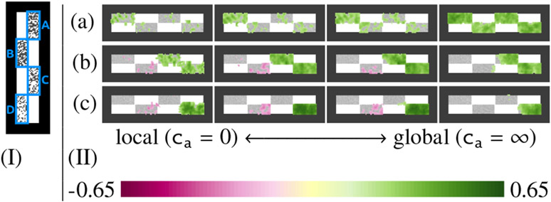
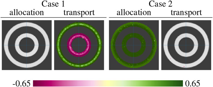
Figure 2 uses a toy example to show the effects of different mass-balancing strategies (different choices of c_a) and different types of tissue loss on the sensitivity of OTF. The example consists of 20 2D images with four rectangular patches that have different amounts of missing tissue. Figure 3 uses another toy example to illustrate that the transport and allocation features can differentiate effects due to change in the location of mass from effects due to overall mass. The example consists of 40 2D images with two concentric annuli that have different amounts of mass (gray scale intensity).

Fig. 2.

A toy example simulating tissue deterioration to illustrate the behaviour of the continuum from local to global mass-balancing. (I) Input image example; each of the regions (A,B,C,D) has various random amounts of white pixels removed, representing tissue deterioration. (II) Suppose that there is a disease (a) corresponding to tissue loss in regions A+B+C+D, a disease (b) corresponding to tissue loss in regions C+D, and a disease (c) corresponding to tissue loss in region D. Here we display the correlation of each disease with the mass allocation OTF at each voxel, and we do this for various choices of c_a. The results illustrate that global mass-balancing leads to stronger correlations compared to local mass-balancing for tissue loss over a large region. However, if only a local region is affected as in (c) and there is confounding (i.e. uncorrelated) tissue loss in other regions, the correlation strength decreases compared to the more local approaches.

Fig. 3.

Correlation to allocation and transport features in two cases on a toy example. In Case 1, each sample image has the same overall mass, but the mass is differently distributed among the two annuli. Color shows correlation between the total mass of the outer annulus and the OTF (mass allocation and transport cost) at each pixel. We see that OTF correctly identified that the effect is due to a trade-off in mass between the inner and outer annuli, and not due to random variation of total mass. There is a statistically significant correlation to transport, but not to allocation. In Case 2, each sample image has a random overall mass which is randomly distributed between the two annuli. Color shows correlation between the total mass of both annuli and the OTF at each pixel. We see that OTF correctly identified the overall difference in mass.

In addition to defining transport and allocation images, optimal transport may also be used to define a notion of distance between two images. The unbalanced optimal transport distance between two images is defined to be the minimum value achieved by the objective on the right hand side of (5). This provides an interesting alternative way to construct a template image, described in (2).

4. Statistical Analysis

This section provides an analysis of the asymptotic correlation strength improvement of OTF over VBM for spatially dispersed effects. We analytically derive Pearson’s correlation coefficients for a pathology scenario with dispersed tissue loss with and without the OTF, showing that OTF significantly improve correlation strength. In Section 4.2 we illustrate the results of the analysis on a toy example that demonstrates the effect of sample size and smoothing on correlation strength.

4.1. Analysis of Correlation Strength

Consider a study with participants that have a pathology with probability p and are healthy with probability 1 − p. We encode this in the random variable H with Bernoulli distribution: the probability of observing a healthy participant is P(H = 1) = 1 − p and the probability of observing a pathological participant is P(H = 0) = p. The effect of the pathology is a tissue loss in some region of the brain. We model the region here as n discrete locations, e.g. the voxels of a brain MRI. We model tissue loss as follows: the probability of observing tissue at a location X is P(T_X = 1∣H = 1) = t_h for the healthy population and P(T_X = 1∣H = 0) = t_p for the pathological population. We assume that these probabilities do not vary with X, i.e., they are the same for each of the n voxel locations.

The correlation between pathology indicator H and tissue expression T_X is

$$\text{cor}(T_X,H)=\frac{E[T_{X}H]-E[T_X]E[H]}{{\sigma }^2(T_X){\sigma }^2(H)}$$ (6)

with E[] the expectation and ${\sigma }^2(T_X)=E[T_X^2]-E[T_X{]}^2$ the variance. The correlation cor(T_X, H) is asymptotically the correlation estimated by VBM at voxel X. The correlations for the VBM approach cor(T_X, H), which may be computed from the distribution of the population P(H) and the conditional tissue loss probabilities P(T_X = 1∣H = 1) = t_h and P(T_X = 1∣H = 0) = t_p.

OTF consist of two features at each voxel: the transport cost image and the mass allocation image. We will focus on the latter and assume that there is no transport, as is the case in the limit of local mass balancing, where c_a ⪡ c. Determining the asymptotic correlation strength for OTF requires computing the probability of allocating or removing tissue amount A_X at a location X for both the healthy and the pathological population: P(A_X∣H = 1) and P(A_X∣H = 0). We compute the allocation and removal probabilities with respect to a template that is constructed by averaging the healthy population: T(X) = E[T_X∣H = 1] = t_h. For the analysis assume that the OTF exclusively allocate or remove tissue and never combine these operations at an individual location. Then the probability of allocating A_X = a units of tissue is zero except when a = −t_h or a = 1 − t_h; i.e., either t_h tissue is removed or 1 − t_h tissue is added. The distribution A_X depends on the total tissue k of the participant. For k > nt_h the probability of allocating tissue at the location X is $\frac{k-n{t}_h}{n(1-t_h)}$ and for k < nt_h the probability of removing tissue is $\frac{t_{h}n-k}{n{t}_h}$. The probability of a participant having tissue at k locations, P(M = k), is binomial distributed with n trials and probability of success t_h and t_p for the healthy and pathological participants, respectively, i.e. M∣(H = 1) ~ B(n, t_h) and M∣(H = 0) ~ B(n, t_p). With this model we can compute the probability of removing or allocating tissue as:

$$\begin{gathered} P(A_X=-t_h\mid H=1)=\sum _{k=1}^{\lfloor t_{h}n\rfloor }P(M=k\mid H=1)\frac{t_{h}n-k}{n{t}_h} \\ P(A_X=1-t_h\mid H=1)=\sum _{k=\lceil t_{h}n\rceil }^{n}P(M=k\mid H=1)\frac{k-t_{h}n}{n(1-t_h)} \\ P(A_X=-t_h\mid H=0)=\sum _{k=1}^{\lfloor t_{h}n\rfloor }P(M=k\mid H=0)\frac{t_{h}n-k}{n{t}_h} \\ P(A_X=1-t_h\mid H=0)=\sum _{k=\lceil t_{h}n\rceil }^{n}P(M=k\mid H=0)\frac{k-t_{h}n}{n(1-t_h)} \end{gathered}$$

The expectations E[A_XH], E[A_X] and $E[A_X^2]$ needed to compute the correlation cor(A_X, H) are readily obtained.

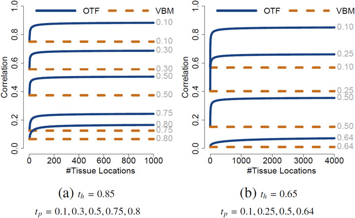
Figure 4 illustrates the effect of OTF on asymptotic correlation strength by plotting cor(T_X, H) and cor(A_X, H) as a function of the number of tissue locations n, i.e. how dispersed the pathology is, for varying parameters. Including OTF in the voxel-wise morphometric analysis increases correlation strength with increasing number of tissue locations. With increasing number of locations, the expected total tissue difference is increased resulting in more locations that require tissue removal. On the other hand, if there are local variations in the populations independent of total tissue loss or gain, then OTF can decrease in statistical power.

Fig. 4.

Plots of the correlation strength for the analysis described in the text. Correlation as a function of the number of tissue locations with (a) t_h = 0.85 and (b) t_h = 0.65 and varying t_p for p = 0.5. The OTF extraction step improves correlation for dispersed tissue loss: An increasing number of locations with tissue loss increases the correlation strength when using OTF.

4.2. Effects of Smoothing and Sample Size

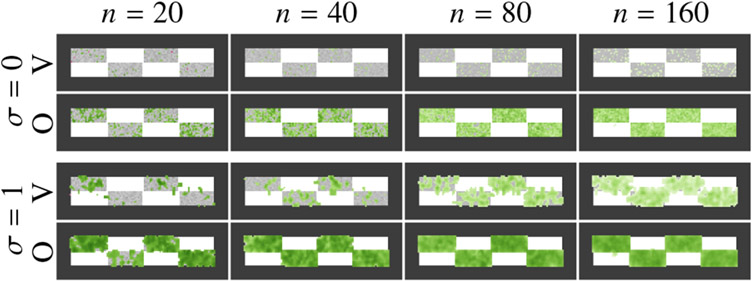
The VBM method requires smoothing in order to convert a tissue mask into a measure of tissue concentration. The smoothing kernel for VBM needs to be large in order to increase the dependency of neighboring voxels and capture effects that vary in their spatial location. While TBM does not need smoothing, it is helpful in terms of statistical sensitivity, and a large smoothing kernel becomes necessary as well if one wants to capture spatially varying effects. The OTF method increases statistical power for diffuse tissue loss and can mitigate effects caused by shifts. However, the exact location for mass allocation is still variable for each image. Thus, the OTF analysis should still employ smoothing to increase spatial dependencies, but it should do so after the computation of the optimal transport solutions. Smoothing is applied to the mass allocation and transport cost images and not to the input images. At this stage the smoothing has the same effect as smoothing for VBM and increases correlation strength at the cost of spatial resolution. Figure 5 empirically illustrates the interaction of sample size and smoothing for OTF and VBM on the toy example from Figure 2.

Fig. 5.

Effects of smoothing and sample size on correlation of features to total mass. The sample images are generated as in Figure 2, and we look at two types of features: VBM (V), which considers voxel intensities, and OTF (O) which produces a mass allocation image out of a solution to the unbalanced optimal transport problem. The correlation strength is indicated in green at locations with statistical significance p < 0.05. VBM requires a large amount of smoothing (σ) and more samples (n) to find statistically significant correlations and results in weaker correlations than OTF with less smoothing and fewer samples. However, OTF with large smoothing can result in a loss of spatial resolution, which leads to the inclusion of large amounts of healthy tissue.

VBM requires a significant amount of smoothing for small to moderate sample size to discover diffuse tissue loss effects. Using OTF detects disperse tissue loss for small samples with little smoothing. We suggest using a truncated Gaussian, or any other kernel with limited range, in order to limit the spatial extent to which signals can be correlated due to smoothing. For large amounts of smoothing, even with a truncated kernel, the smoothing can yield false positive correlations, as shown in Figure 5 where the effects leak into the healthy white regions.

5. Results

We demonstrate the effect of OTF on the OASIS-1 data. The OASIS-1 data set was collected for studying the effects of cognitive impairment. The OASIS-1 database consists of T1-weighted MRI and tissue segmentation masks of 416 participants aged 18 to 96 (Marcus et al., 2010). The images in the OASIS-1 data set are brain-extracted, gain-field corrected, and registered to the Talaraich atlas space (Talairach and Tournoux, 1988) with an affine transform.

The OASIS-1 data set has a clinical dementia rating (CDR) associated to each participant. We restrict the analysis to 177 participants aged sixty and over to reduce the effects of age. The clinical dementia rating of the 177 participants falls into 3 categories: healthy (CDR = 0, 90 participants), very mild (CDR = 0.5, 60 participants), mild (CDR = 1, 25 participants), and moderate dementia (CDR = 2, 2 participants). Figure 6 shows histograms of age for each CDR rating of the population used in this analysis.

Fig. 6.

Histogram of ages per CDR group of the OASIS-1 data.

5.1. Analysis Methodology

To explore the effect of the optimal transport feature extraction in both the VBM and TBM setting we registered the T1-weighted images to the SRI24 atlas (Rohlfing et al., 2010) using an affine registration followed by SyN diffeomorphic registration (Avants et al., 2008), a state-of-the-art non-parametric registration method. For the VBM analysis we align the tissue segmentations to SRI24 with the affine registration only; we will refer to this as VBM-Aff. For the TBM analysis we align the tissue segmentations to SRI24 with an affine plus nonlinear warp and multiply the segmentation masks by the Jacobian determinant of the nonlinear warp to correct for volume changes (Ashburner, 2007). The final pipeline for our TBM analysis can be summarized as follows:

1. Preprocess (brain extraction and bias correction).

2. Register each image to the SRI24 atlas via SyN.

3. Segment each aligned image to obtain a gray matter mask.

4. Take the Jacobian determinant of the deformation that aligned each image and restrict it to the gray matter mask. The resulting tissue density maps X_k are the main input into the optimal transport analysis pipeline.

5. Construct a template T out of the X_k by taking either the sparse Euclidean mean or the optimal transport barycenter.

6. Solve the unbalanced optimal transport problem from T to X_k for each k. We do this by setting up the linear program (5) as a minimum cost flow problem (Ahuja et al., 1993) and taking a multiscale approach (Gerber and Maggioni, 2017).

7. Compute the OTF, i.e. the mass allocation images M_k and the transport cost images C_k.

8. Compute the voxel-wise correlation of M_k and C_k with a target variable of interest, creating correlation images like the ones seen in Figures 1, 2, 3, 5, 7, 8, 9, and 10.

Fig. 7.

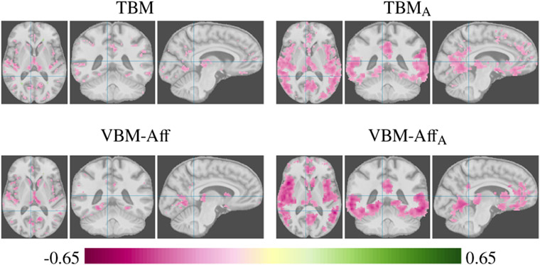
TBM and VBM analysis of gray matter tissue without and with the optimal transport feature extraction step. The color shows inverse correlation strength (pink) to clinical dementia rating for voxels with Bonferroni corrected p < 0.05.

Fig. 8.

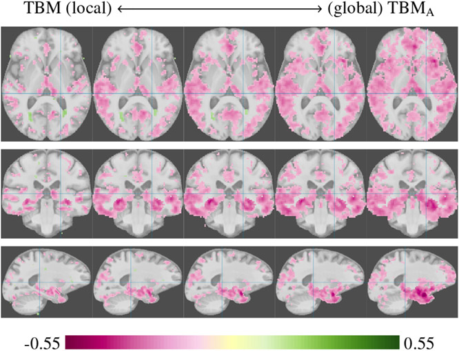
Inverse correlations of gray matter to CDR, illustrating the continuum from TBM analysis to TBMA with global mass balancing. From left to right the cost of allocating mass is increased, causing a more global mass balancing to be enforced. The global TBMA analysis can mask local effects if there is no overall difference in tissue loss between the populations. Performing the analysis at different spatial scales improves the odds of discovering local and global effects.

Fig. 9.

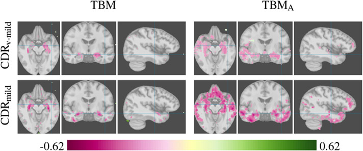
Axial, coronal, and sagittal slices show the inverse correlation of gray matter tissue to very mild (CDR_v-mild) and mild dementia (CDR_mild).

Fig. 10.

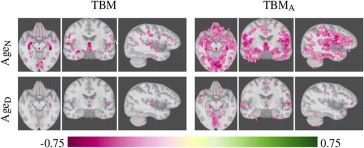
Axial, coronal, and sagittal slices show the inverse correlation of gray matter tissue to age that is associated to normal aging (Age_N) and to age within the dementia group (Age_D).

We apply VBM and TBM analysis to gray matter tissue masks with respect to several different variables and subpopulations:

• Age_N: Age for participants with CDR = 0, to explore the effects of normal aging.

• Age_D: Age for participants with CDR > 0, to explore the effects of aging in the cognitively impaired population. CDR and age for this group have a weak correlation of 0.18 with a p-value of 0.13, suggesting that any effects discovered in this group are not related to CDR rating.

• CDR: CDR rating on all participants, to explore the overall effect of cognitive impairment.

• CDR_v-mild : Binary variable of CDR 0 versus CDR 0.5 participants, to explore the effects of cognitive impairment at a very early stage.

• CDR_mild : Binary variable of CDR 0 versus CDR 1 participants, to explore the effects of the progression of cognitive impairment by comparing to the CDR 0.5 group.

In all figures we show correlation strength at all locations with Bonferroni corrected p < 0.05.

We constructed mass allocation and transport cost images for both the TBM and VBM-Aff approach which we will refer to as TBM_A, TBM_T and VBM-Aff_A, VBM-Aff_T, respectively.

The mass allocation and transport cost images are obtained as described in Section 3.3 by computing transport maps to a sparse Euclidean mean template. The template is constructed as described in Section 3.1 using s = 0.9n, where n is the number of images in the data set. For the brain images, the optimal transport mean and the sparse Euclidean mean resulted in small differences and did not affect the qualitative results. For the transport cost c we use the squared Euclidean distance between the voxel locations to introduce a preference of many small mass transfers over fewer larger mass transfers. To reduce computation costs the images are downsampled by a factor of 2, leading to a resolution of 88 × 104 × 88 voxels with a voxel size of 2 × 2 × 2 mm. The downsampling resulted in computation times of approximately one to two hours per optimal transport problem when using a multiscale optimal transport solver (Gerber and Maggioni, 2017).

Software to replicate the results can be found on github¹. The github repository also contains links to interactive web visualizations of the results presented here.

5.2. Non-linear TBM and Affine Only VBM Analysis

Figure 7 illustrates the effects of using TBM and with and without OTF. The use of affine registration in the VBM case is a simple way to ensure that local structures are not aligned so perfectly as to wash out the signal that can be observed by VBM. If we try to align each gyrus and sulcus, as we do with non-parametric registration, then it becomes more appropriate to use TBM (Frackowiak, 2004, Chaper 7). We should expect similar results from TBM and VBM-Aff and similar results from TBM_A and VBM-Aff_A. This is because the Jacobian determinant of the non-parametric registration will deviate from 1 (i.e. indicate contractions or expansions) near tissue boundaries, and this is exactly where the affine registration is expected to be mismatched. Using OTF has the same effect in both settings with stronger correlations over larger regions. The results show the increased statistical power provided by OTF and the capability to compensate for shifts in exact tissue location due to registration mismatches.

5.3. Local to Global Analysis

Figure 8 illustrates the continuum from local (TBM) to global (TBM_A) mass-balancing strategies, as described in Section 3.2, on an analysis of correlation of gray matter amount to CDR. The global versus local analysis has two complementary effects. For pathologies that result in a widespread tissue loss with large individual variation in the exact location of tissue loss, the global analysis will increase correlation strength and potentially discover effects not apparent with a local analysis. On the other hand, if the pathology has locally concentrated effects, large individual variations in total volume can mask this effect in the global analysis and a more local analysis would be needed. Figure 8 shows some of these effects. We suggest running OTF analysis at multiple scales, as shown in Figure 8, and comparing the results to get a more complete picture of potential effects.

The global analysis discovers a more widespread loss of tissue (negative correlation), particularly in the temporal lobes, not visible with a local analysis. The local analysis shows a tissue gain near the ventricles. A tissue gain in the cortex is unlikely and this effect could be due to CSF appearing brighter in participants with CDR > 0 and being misclassified as gray matter. This effect disappears with the global analysis; the overall loss of gray matter is a much stronger effect than the localized tissue gain.

5.4. Increase in Statistical Power

Figure 9 shows the results of a TBM analysis of mild and very mild dementia with and without OTF, demonstrating the increased statistical power that OTF provide for spatially dispersed effects. TBM_A finds correlations with cognitive impairment in the temporal lobe but also the occipital, parietal, and frontal lobe, that are not detected by a TBM analysis without the OTF extraction step. The findings are consistent with results from the literature (Burton et al., 2004; Kaye et al., 1997; Brun, 1987) that report gray matter loss in the frontal, temporal, and occipital lobe. The disease progression from CDR 0.5 to CDR 1 indicated by OTF analysis resembles the Braak stages from autopsies (Braak and Braak, 1991) that reveal a spread from the limbic regions in the early stages to the neocortex in the later stages. In particular the amyloid deposit stages B and C and the intra-neuronal neurofibrillary changes stages III-IV and V-VI match the OTF analysis findings for participants with very mild and mild dementia, respectively.

For aging, see Figure 10, TBM_A detects tissue loss in the area around the postcentral gyrus. The primary somatosensory cortex, located in this region, has been reported to correlate with age-related tissue loss (Raz et al., 1997). TBM_A also shows loss of tissue in the cerebellum, reported as being significantly correlated with aging in prior manual studies (Jernigan et al., 2001; Luft et al., 1999).

The effects of normal aging and dementia differ and suggest that normal aging is not on a continuum with dementia-related aging, but is rather a separate process. Interestingly the effects of aging in the dementia group are less pronounced than in the normal aging group, potentially suggesting that dementia effects mask typical aging processes.

The TBM_A analysis suggests that aging in individuals with very mild or mild dementia progresses drastically differently from normal aging. This difference is not clearly discernible in the VBM-Aff analysis. Furthermore, the effects of aging in the dementia group (Figure 10, bottom) are different from the effects of the progression of cognitive impairment (Figure 9). This could indicate that the CDR scale is not sensitive to gray matter reductions in certain regions and hence does not show a relationship within the normal aging group.

5.5. Separating Differences in Tissue Location Versus Volume

Figure 11 shows correlation of white matter tissue to age for TBM, TBM_T, and TBM_A. Correlation with transport cost (TBM_T) indicates a consistent difference in shape or distribution of tissue location, while correlation with mass allocation (TBM_A) indicates differences in the amount of tissue. The TBM_T results indicate that some of the correlation displayed by TBM can be explained by differences in anatomical shape and are not necessarily associated with tissue loss: The tissue gain around the ventricles and the occipital region in TBM can be attributed to persistent difference in tissue location and does not correspond to tissue loss. This conclusion is based on comparing transport cost (TBM_T) correlation to the TBM findings: Regions where the transport cost correlations overlap with the TBM results suggest that the TBM results are due to anatomical shape differences and/or due to effects of the spatial alignment. Even with a highly nonlinear warp, the registration step is driven by tissue boundaries and leads to Jacobian determinants that are dominant around anatomical boundaries. For a shift in boundaries, this results in a contraction and an expansion on opposite sides. OTF analysis is not sensitive to shifts and mitigates this effect.

Fig. 11.

Axial and coronal slices displaying the results of TBM, transport cost (TBM_T), and mass allocation (TBM_A) analysis of white matter with respect to Age. TBM_T indicates that some of the correlations in TBM, in particular the correlations around the ventricles and in the posterior, are potentially caused by differences in tissue locations between the populations and not changes in tissue amounts.

6. Conclusion

The work provides evidence that optimal transport features increase the statistical power of morphometric analysis for spatially dispersed effects. Optimal transport features capture regional and global changes while retaining the benefits of a voxel-wise visualization and analysis of results. We demonstrate that OTF can attribute effects to either mass transfer, due to anatomical variations in shape or misalignment, or mass allocation, due to volume differences. Statistical assessment demonstrates that for diffuse tissue loss OTF analysis increases correlation strength. The mass-balancing, introduced in Section 3.2, links the OTF to VBM/TBM through a continuum that enhances identification of effects from localized to globally dispersed.

An important step for future work is to integrate OTF to surface based morphometric analysis. An open challenge is to consider how to apply OTF to the analysis of functional brain images (fMRI) and other time-varying measurements.

References

- Ahuja RK, Magnanti TL, Orlin JB, 1993. Network Flows: Theory, Algorithms, and Applications. Prentice-Hall, Inc., Upper Saddle River, NJ, USA. [Google Scholar]
- Anderes E, Borgwardt S, Miller J, 2016. Discrete wasserstein barycenters: Optimal transport for discrete data. Mathematical Methods of Operations Research 84, 389–409. [Google Scholar]
- Ashburner J, 2007. A fast diffeomorphic image registration algorithm. Neuroimage 38, 95–113. [DOI] [PubMed] [Google Scholar]
- Ashburner J, Friston KJ, 2000. Voxel-based morphometry—the methods. Neuroimage 11, 805–821. [DOI] [PubMed] [Google Scholar]
- Ashburner J, Hutton C, Frackowiak R, Johnsrude I, Price C, Friston K, et al. , 1998. Identifying global anatomical differences: deformation-based morphometry. Human brain mapping 6, 348–357. [DOI] [PMC free article] [PubMed] [Google Scholar]
- Avants BB, Epstein CL, Grossman M, Gee JC, 2008. Symmetric diffeomorphic image registration with cross-correlation: evaluating automated labeling of elderly and neurodegenerative brain. Medical image analysis 12, 26–41. [DOI] [PMC free article] [PubMed] [Google Scholar]
- Benamou JD, 2003. Numerical resolution of an “unbalanced” mass transport problem. ESAIM: Mathematical Modelling and Numerical Analysis 37, 851–868. [Google Scholar]
- Benamou JD, Brenier Y, 2000. A computational fluid mechanics solution to the monge-kantorovich mass transfer problem. Numerische Mathematik 84, 375–393. [Google Scholar]
- Bookstein FL, 2001. “voxel-based morphometry” should not be used with imperfectly registered images. Neuroimage 14, 1454–1462. [DOI] [PubMed] [Google Scholar]
- Braak H, Braak E, 1991. Neuropathological stageing of alzheimer-related changes. Acta neuropathologica 82, 239–259. [DOI] [PubMed] [Google Scholar]
- Brun A, 1987. Frontal lobe degeneration of non-alzheimer type. i. neuropathology. Archives of gerontology and geriatrics 6, 193–208. [DOI] [PubMed] [Google Scholar]
- Burton EJ, McKeith IG, Burn DJ, Williams ED, O’Brien JT, 2004. Cerebral atrophy in parkinson’s disease with and without dementia: a comparison with alzheimer’s disease, dementia with lewy bodies and controls. Brain 127, 791–800. [DOI] [PubMed] [Google Scholar]
- Chizat L, Peyré G, Schmitzer B, Vialard FX, 2018. Unbalanced optimal transport: Dynamic and kantorovich formulations. Journal of Functional Analysis 274, 3090–3123. [Google Scholar]
- Cuturi M, 2013. Sinkhorn distances: Lightspeed computation of optimal transport, in: Advances in neural information processing systems, pp. 2292–2300. [Google Scholar]
- Cuturi M, Doucet A, 2014. Fast computation of wasserstein barycenters, in: International Conference on Machine Learning, pp. 685–693. [Google Scholar]
- Dale AM, Fischl B, Sereno MI, 1999. Cortical surface-based analysis: I. segmentation and surface reconstruction. Neuroimage 9, 179–194. [DOI] [PubMed] [Google Scholar]
- Davatzikos C, 2004. Why voxel-based morphometric analysis should be used with great caution when characterizing group differences. Neuroimage 23, 17–20. [DOI] [PubMed] [Google Scholar]
- Feydy J, Charlier B, Vialard FX, Peyré G, 2017. Optimal transport for diffeomorphic registration, in: International Conference on Medical Image Computing and Computer-Assisted Intervention, Springer. pp. 291–299. [Google Scholar]
- Frackowiak RS, 2004. Human brain function. Academic press. [Google Scholar]
- Gangbo W, Li W, Osher S, Puthawala M, 2019. Unnormalized optimal transport. Journal of Computational Physics 399, 108940. [Google Scholar]
- Gerber S, Maggioni M, 2017. Multiscale strategies for computing optimal transport. Journal of Machine Learning Research 18, 1–32. [Google Scholar]
- Gerber S, Niethammer M, Styner M, Aylward S, 2018. Exploratory population analysis with unbalanced optimal transport, in: International Conference on Medical Image Computing and Computer-Assisted Intervention, Springer. pp. 464–472. [DOI] [PMC free article] [PubMed] [Google Scholar]
- Gramfort A, Peyré G, Cuturi M, 2015. Fast optimal transport averaging of neuroimaging data, in: International Conference on Information Processing in Medical Imaging, Springer. pp. 261–272. [DOI] [PubMed] [Google Scholar]
- Guittet K, 2002. Extended Kantorovich norms: a tool for optimization. Ph.D. thesis. INRIA. [Google Scholar]
- Hua X, Leow AD, Parikshak N, Lee S, Chiang MC, Toga AW, Jack CR Jr, Weiner MW, Thompson PM, Initiative ADN, et al. , 2008. Tensor-based morphometry as a neuroimaging biomarker for alzheimer’s disease: an mri study of 676 ad, mci, and normal subjects. Neuroimage 43, 458–469. [DOI] [PMC free article] [PubMed] [Google Scholar]
- Jernigan TL, Archibald SL, Fennema-Notestine C, Gamst AC, Stout JC, Bonner J, Hesselink JR, 2001. Effects of age on tissues and regions of the cerebrum and cerebellum. Neurobiology of aging 22, 581–594. [DOI] [PubMed] [Google Scholar]
- Kaye JA, Swihart T, Howieson D, Dame A, Moore M, Karnos T, Camicioli R, Ball M, Oken B, Sexton G, 1997. Volume loss of the hippocampus and temporal lobe in healthy elderly persons destined to develop dementia. Neurology 48, 1297–1304. [DOI] [PubMed] [Google Scholar]
- Kundu S, Kolouri S, Erickson KI, Kramer AF, McAuley E, Rohde GK, 2018. Discovery and visualization of structural biomarkers from mri using transport-based morphometry. NeuroImage 167, 256–275. [DOI] [PMC free article] [PubMed] [Google Scholar]
- Lee W, Lai R, Li W, Osher S, 2021. Generalized unnormalized optimal transport and its fast algorithms. Journal of Computational Physics 436, 110041. [Google Scholar]
- Liero M, Mielke A, Savaré G, 2017. Optimal entropy-transport problems and a new hellinger–kantorovich distance between positive measures. Inventiones mathematicae 211, 969–1117. [Google Scholar]
- Luft AR, Skalej M, Schulz JB,Welte D, Kolb R, Bürk K, Klockgether T, Voigt K, 1999. Patterns of age-related shrinkage in cerebellum and brainstem observed in vivo using three-dimensional mri volumetry. Cerebral Cortex 9, 712–721. [DOI] [PubMed] [Google Scholar]
- Marcus DS, Fotenos AF, Csernansky JG, Morris JC, Buckner RL, 2010. Open access series of imaging studies: longitudinal mri data in non-demented and demented older adults. Journal of cognitive neuroscience 22, 2677–2684. [DOI] [PMC free article] [PubMed] [Google Scholar]
- Mérigot Q, Thibert B, 2021. Optimal transport: discretization and algorithms, in: Geometric Partial Differential Equations - Part II. Elsevier, pp. 133–212. [Google Scholar]
- Prakash A, Balakrishna U, Thenepalle JK, 2022. An exact algorithm for constrained k-cardinality unbalanced assignment problem. International Journal of Industrial Engineering Computations 13, 267–276. [Google Scholar]
- Raz N, Gunning FM, Head D, Dupuis JH, McQuain J, Briggs SD, Loken WJ, Thornton AE, Acker JD, 1997. Selective aging of the human cerebral cortex observed in vivo: differential vulnerability of the prefrontal gray matter. Cerebral cortex (New York, NY: 1991) 7, 268–282. [DOI] [PubMed] [Google Scholar]
- Rohlfing T, Zahr NM, Sullivan EV, Pfefferbaum A, 2010. The sri24 multichannel atlas of normal adult human brain structure. Human brain mapping 31, 798–819. [DOI] [PMC free article] [PubMed] [Google Scholar]
- Scarpazza C, De Simone MS, 2016. Voxel-based morphometry: current perspectives. Neuroscience and Neuroeconomics 5, 19–35. [Google Scholar]
- Talairach J, Tournoux P, 1988. Co-planar stereotaxic atlas of the human brain. 3-Dimensional proportional system: an approach to cerebral imaging. Thieme, New York. [Google Scholar]