

Abstract

Rate of penetration (ROP) is an essential factor in drilling optimization and reducing the drilling cycle. Most of the traditional ROP prediction methods are based on building physical model and single intelligent algorithms, and the efficiency and accuracy of these prediction methods are very low. With the development of artificial intelligence, high-performance algorithms make reliable prediction possible from the data perspective. To improve ROP prediction efficiency and accuracy, this paper presents a method based on particle swarm algorithm for optimization of long short-term memory (LSTM) neural networks. In this paper, we consider the Tuha Shengbei block oilfield as an example. First, the Pearson correlation coefficient is used to measure the correlation between the characteristics and eight parameters are screened out, namely, the depth of the well, gamma, formation density, pore pressure, well diameter, drilling time, displacement, and drilling fluid density. Second, the PSO algorithm is employed to optimize the super-parameters in the construction of the LSTM model to the predict ROP. Third, we assessed model performance using the determination coefficient (R2), root mean square error (RMSE), and mean absolute percentage error (MAPE). The evaluation results show that the optimized LSTM model achieves an R2 of 0.978 and RMSE and MAPE are 0.287 and 12.862, respectively, hence overperforming the existing methods. The average accuracy of the optimized LSTM model is also improved by 44.2%, indicating that the prediction accuracy of the optimized model is higher. This proposed method can help to drill engineers and decision makers to better plan the drilling operation scheme and reduce the drilling cycle.
1. Introduction
The rate of penetration (ROP) represents the drilling footage per unit of pure drilling time. The higher the ROP, the higher the drilling efficiency and speed.1,2 To effectively manage the drilling operation, engineers must consider the ROP in advance. Currently, ROP prediction is mainly performed based on the expertise of the field engineers and analyzing the post-drilling data; hence, it is often subjective and unreliable.3 Accurate prediction of ROP results in effective evaluation of the drilling cycle and its cost,4,5 thus acting as an essential means enabling engineers to effectively design and improve the drilling speed.6,7 Existing research on ROP prediction of drilling machinery can be categorized into the following three stages. From the 1950s to the 1990s, the ROP equation was mainly obtained by building a physical model. For instance, Walker et al. and Guo8,9 obtained the ROP equation based on a regression method considering the mechanical parameters of the rocks and the drilling parameters, e.g., weight on bit (WOB), rotational speed, and displacement. Mobeen et al. and Zeeshan et al.10,11 have carried out a lot of laboratory experiments to measure the compressive strength and tensile strength of cement slurry solidified under high temperature. Anemangely et al.12 determined the constant coefficients of Bourgoyne and Young drilling rate models using an evolutionary algorithm. Physical models based on field data and relevant factor regression can only be used for drilling analysis after drilling; hence, the corresponding stratum is narrow and the accuracy is not high. Therefore, it is often difficult to obtain the required field drilling data, hence significantly affecting the optimization of integrated and efficient drilling schemes.
An example of the methods used from the end of the 20th century to the beginning of the 21st century is presented in Deng et al.13 In this work, the rock breaking process of the drill bit is simulated on the computer to quantitatively determine ROP. Furthermore, Lin et al.14 predicted the ROP of percussion rotary drilling machinery using a computer simulation method. Computer simulation simplifies the problem, saves manpower and material resources, and does not require a large number of field data. Nevertheless, the simulation parameters need to be verified by experiments. In addition, the models have limitations reducing the ROP prediction efficiency.
The rapid development of artificial intelligence technology has enabled the implementation of more accurate prediction methods. Many researchers used intelligent algorithms for ROP prediction. For instance, Yan et al. and Amer et al.15,16 proposed a new method for predicting ROP based on an artificial neural network model. Also, Song et al.17 devised the intelligent prediction of ROP based on support vector machine (SVM) regression. Another example of such approaches is Ahmed et al.18 where the feasibility of ROP prediction based on intelligent algorithms was investigated by analyzing the prediction accuracy of intelligent models such as artificial neural networks and SVM. Al-Gharbi et al. and Elkatatny et al.19,20 performed real-time prediction using artificial neural networks; the results show that the developed model is a robust technique and tool that can be used to predict the real-time drilling fluid rheological parameters. Elkatatny et al.21 used more than 600 measured core data points to build an AI model; the results show that AI techniques can be used to predict parameter and the correlation based on the optimized model can predict the parameter with high accuracy. Mand et al. and Ayyaz et al.22,23 performed shale brittleness prediction and generation of synthetic photoelectric log using the machine learning approach; the effective use of an artificial neural network shows that the existing data repository can be used to generate logging accurately, and the results show that the artificial neural network was found to have high accuracy.
Furthermore, Mahmoud et al.24 applied machine learning to acid cracking test data points to establish several conductivity correlations and proposed an artificial neural network model to predict the fracture conductivity of carbonate rocks and pointed out that all AI models are data driven. Tariq et al. and Mustafa et al.25,26 used data-driven machine learning to predict fracture pressure and mineralogy. Anemangely et al. and Bajolvand et al.27,28 performed drilling rate prediction with the multilayer perceptron neural network and convolutional neural network, and these methods illustrate that the application of artificial neural models for ROP prediction is a feasible and useful method. Wang et al.29 used particle swarm optimization to optimize the intelligent model for shear wave velocity prediction. Bajolvand et al.30 optimized drilling parameters based on geomechanics, and the optimization technique of geomechanics successfully improved the performance of drilling operations, and these optimization examples show that parameter optimization is necessary for performance improvement. Their analysis confirmed the accuracy of particle swarm optimization in model parameter optimization. Most of the abovementioned methods for intelligent prediction of ROP are single intelligent algorithms, where the model parameters are set arbitrarily. This results in a long training time, low prediction accuracy, and overfitting in the prediction process.31 The LSTM neural network model in deep learning has high prediction accuracy and can effectively overcome the problems of overfitting in previous methods.32,33 This method is also suitable for predicting the ROP of other oilfields.3
Previous research works also confirmed the efficiency of using the PSO algorithm and LSTM neural networks in solving complex engineering problems.34−39 The PSO algorithm is based on a simple design and provides strong global search ability and fast convergence and hence is often used to solve various complex optimization problems.40,41 In this paper, we use the PSO algorithm to optimize the training parameters in the LSTM model, accelerate the convergence speed of the model, reduce the training time, and improve the prediction accuracy.
To address the issue in the existing ROP prediction methods, we combine the prediction advantages of the PSO optimization algorithm and the LSTM neural network model. In this approach, the LSTM neural network optimized by PSO is used for ROP prediction. The prediction results of the LSTM model before and after optimization are also compared and analyzed. It is verified that the LSTM model optimized by the PSO algorithm has a shorter training time while providing a higher prediction accuracy. This method helps the drilling engineers and decision makers to obtain drilling information in advance and better plan the drilling operations and shorten the process. The proposed method also introduces a new means to predict drilling parameters, which improves the inefficiency and low prediction accuracy of the previous prediction methods.
The main contribution of this paper is to combine the advantages of the PSO optimization algorithm and the LSTM neural network model. We propose an improved LSTM prediction method for ROP prediction. Comparing the LSTM model prediction results before and after optimization shows that the training time of the optimized method is shorter and its accuracy is higher. Our results confirm the feasibility of optimizing the neural network algorithm through the optimization algorithm, hence introducing a new approach that can be applied to other aspects of petroleum engineering.
Figure 1 shows the workflow of the proposed method in this paper. The system includes five main stages: data processing, model building, model optimization, model training, and result evaluation.
Figure 1.
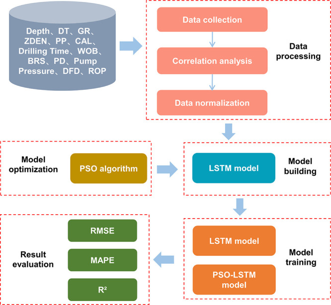
Workflow chart of ROP forecasting.
2. Data Processing
2.1. Data Collection
The data we used in this paper is the well and mud logging data of a drilled section in the Tuha Shengbei block (Figure 2) including a total of 1853 sets of data. The well logging data (Figure 2a) includes the depth of the well (Depth), the acoustic time difference (DT), gamma (GR), formation density (ZDEN), formation pore pressure (PP), and well diameter (CAL), The mud logging data (Figure 2b) also includes drilling time (Drilling Time), WOB, bit speed (BRS), displacement (PD), pump pressure (Pump Pressure), drilling fluid density (DFD), and ROP. Table 1 summarizes the basic information of these parameters, including the unit, minimum value, maximum value, and average value of each parameter.
Figure 2.

Raw collection data. (a) Logging data. (b) Mud-logging data.
Table 1. Statistical Information Table of Original Input Parameters.
| parameter | unit | minimum | maximum | average |
|---|---|---|---|---|
| depth | m | 2640 | 4492 | 3566 |
| DT | μs/ft | 59.59 | 172.53 | 79.26 |
| GR | GAPI | 24.68 | 325.84 | 83.72 |
| ZDEN | g/cm3 | 1.18 | 2.65 | 2.318 |
| PP | g/cm3 | 0.94 | 1.35 | 1.09 |
| CAL | in | 20.48 | 42.79 | 30.69 |
| drilling time | min/m | 1.85 | 129.4 | 18.51 |
| WOB | KN | 20 | 120 | 81.06 |
| BRS | r/min | 73 | 200 | 180.12 |
| PD | L/s | 20 | 50 | 38.38 |
| pump pressure | MPa | 10 | 20 | 17.48 |
| DFD | g/cm3 | 1.2 | 1.52 | 1.38 |
| ROP | m/h | 0.67 | 9.8 | 3.39 |
2.2. Correlation Analysis and Normalization
In the previous methods, the selection of relevant parameters for ROP prediction was often arbitrary and the influence of these parameters on ROP was different. Nevertheless, the correlation between the data will affect the training speed and training effect of the model. Therefore, before model training, it is necessary to conduct a correlation analysis on the input parameters to screen out the parameters with strong correlations. The Pearson correlation coefficient42 is used to measure the correlation between various parameters. The Pearson correlation coefficient expression between X and Y variables is defined as
| 1 |
where is the correlation coefficient with a value range of [−1,1]. A positive (negative) r indicates that the two characteristics are positively(negatively) correlated.
The thermodynamic diagram of the correlation between various parameters is presented in Figure 3. Here, the darker the color, the stronger the positive and negative correlations. Based on this, eight parameters with a strong correlation with ROP are selected as the model input variables, namely, Depth, GR, ZDEN, PP, CAL, Drilling Time, PD, and Drilling fluid density.
Figure 3.

Heat map of correlation between features.
Data normalization results in similar data distribution of each dimension and can avoid the problem of inconsistent gradient decline. It is also conducive to adjusting the learning rate, hence speeding up the search for the optimal solution.43 The input parameters filtered by the correlation analysis are normalized using the following formula:
| 2 |
where xi is the original data, xmin is its minimum value, xmax is its maximum value, and yi is the normalized data, which is in (0,1).
3. Model Building
3.1. LSTM Neural Network
The LSTM neural network was first proposed by Hochreiter and Schmidhuber44 in 1997. It is an optimization algorithm of the traditional recurrent neural network (RNN), which can effectively overcome the problems of memory temporary storage and gradient dispersion in RNN. LSTM has both long-term and short-term memory functions and is widely used in the prediction of time-series problems.45
Depth series and time series are essentially the same, and there is an internal relationship between the previous data point and the next data point.46 Therefore, the LSTM model can be used to predict the penetration rate of deep formations. The LSTM network structure is shown in Figure 4. On the left, the logical architecture diagram of LSTM sequence expansion is presented. This can be expanded along the horizontal (time/depth) sequence and the vertical (interlayer) sequence. On the right is the internal logical relationship diagram of a single LSTM, mainly including forget gate (ft), input gate (it), output gate (ot), and candidate state (ct0).
Figure 4.

Logical structure diagram of the LSTM neural network.
Here, we define W and b as the weight matrix and the offset term of LSTM. Subscripts f, i, and o represent the forget gate, the input gate, and the output gate, respectively:
| 3 |
| 4 |
The implementation process of the LSTM algorithm includes the following three steps. The first step goes through a forgetting gate, which can selectively forget information of the previous time step. This step is implemented by the sigmoid layer defined as
| 5 |
where ft is the forgetting gate, xt represents the input at time t, ht – 1 is the short-term memory at time t, and sigmoid is the activation function. Its output range is [0,1], where 0 represents “completely forgetting all information” and 1 represents “completely retaining all information”. The function expression is
| 6 |
The second step is the input gate, which determines information to be stored in the current time step. This step is implemented by the sigmoid and tanh layers. The sigmoid layer decides to update the information, as shown in eq 7. The tanh layer also creates a new candidate value and adds it to the candidate state (see, eq 8):
| 7 |
| 8 |
where it is the input gate, ct0 is the candidate state, tanh is the Bi tangent activation function, its output range is [−1,1], and the tanh function is defined in the following:
| 9 |
After the above steps, the state ct – 1 of the previous unit is updated to ct, as the following:
| 10 |
where ct is the updated long-term memory and ⊗ is the point-by-point product.
The third step is the output gate, which determines the output of the current state. The sigmoid layer is run to get the output unitl. The unitl state is then gone through tanh and multiplied by the output of the sigmoid gate. Therefore, only the selected part is the output. The calculation process is
| 11 |
| 12 |
where ot is the output gate and ht is the output value of the current cell state.
3.2. PSO Algorithm
PSO was first proposed by Kennedy and Eberhart47 in 1995. It originated from the research on birds’ foraging behavior, birds where they search the surrounding area nearest to food and use their individual flight experience to determine the food location while continuously sharing location information with the rest of the group. This enables the whole group to quickly obtain the optimal solution for the foraging route.48,49
The PSO algorithm regards the individuals in the group as particles searching in space. Each particle is characterized by its position and speed, and its movement pattern is the result of combining the movement trend of the whole group (global search) with its own cognition (local search). In the process of space search, particles constantly track the optimal solution to adjust their parameters to complete the search process from local optimization to global optimization.
Assume that a population of m particles is in an N-dimensional space, X = (x1, x2, ..., xm). The position of a particle i in the N-dimensional space is also represented by Xi = [xi1, xi2, ..., xim]T; its speed is denoted by Vi = [vi1, vi2, ..., vim]T. The individual optimal position is represented by Pi = [Pi1, Pi2, ..., Pim]T, and the global optimal position is Pg = [Pg1, Pg2, ..., Pgm]T. The particle’s speed and position in the search process are
| 13 |
| 14 |
where w is the inertia weight, which is used to control the weight distribution of the particles in the local optimization and the global optimization; c1 and c2 are the acceleration factors that are used to adjust the flight step size, which have generally nonnegative values. The values of r1 and r2 are random numbers between [0,1]; Vink, Xin, Pink, and Pgnare the local and globally optimal solutions of the particle’s speed and position at the corresponding time.
The workflow of the PSO algorithm is shown in Figure 5. Since the PSO algorithm is simple and provides strong global search ability and fast convergence speed, it is often used to solve various complex optimization problems. To see the details of finding the optimal solution of parameters, see ref (50).
Figure 5.
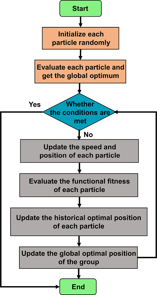
Workflow of particle swarm optimization algorithm.
3.3. LSTM Based on Particle Swarm Optimization
Conventionally, most of the ROP prediction methods are single intelligent prediction techniques, where the model parameter values are randomly set, resulting in a long training time and low prediction accuracy. PSO is an effective method to optimize complex parameter values, has good learning ability, and has been used to solve complex optimization problems in various fields.51,52
The network construction, training process, and result prediction in this paper were all carried out in MATLAB 2021b. The software package has a deep learning toolkit that can be used to choose the sequence-to-sequence network in the deep network designer to build the LSTM neural network layer. This network is then used for encoding or decoding and conversion together with the LSTM. The processes of building the LSTM neural network layer set the function parameters’ values. The super-parameters of the model have great influence on the convergence speed and accuracy of the ROP prediction model during training.53−55
In this paper, the method of combining the particle swarm optimization algorithm and the LSTM neural network is to optimize the four main super-parameters of LSTM. These parameters are the number of neurons in the hidden layer (Numhiddenunits), the learning rate (Initiallearnrate), the number of iterations (Maxepoch), and the minimum training batch (Minbatchsize). They are used as the optimization variables of the particle swarm optimization algorithm. By updating the speed and position of particles, better model parameters are obtained. The variable values before and after the optimization of the LSTM network layer function are shown in Table 2. The LSTM physical model architecture of particle swarm optimization is also depicted in Figure 6. First the input data then the PSO algorithm in the training process optimizes the four hyper-parameters of the LSTM neural network model and finally outputs the prediction results of the ROP.
Table 2. Variable Values before and after Optimization of the LSTM Network Layer Functions.
| function | variable | value before optimization | optimized value | describe |
|---|---|---|---|---|
| sequenceInputLayer | InputSize | 9 | 9 | number of input parameters |
| MinLength | 1 | 1 | minimum input length of data | |
| lstmLayer | InputSize | auto | auto | automatic adjustment |
| NumHiddenUnits | 100, 50 | 128, 64 | LSTM hidden layer | |
| Bias | 32 | 32 | offset term | |
| dropoutLayer | dropout | 0.2 | 0.2 | probability of node dropping |
| fullyConnectedLayer | OutputSize | 1 | 1 | number of output parameters |
| regressionLayer | regression output | |||
| trainingOptions | MaxEpochs | 100 | 50 | number of training set runs |
| InitialLearnRate | 0.005 | 0.001 | learning rate | |
| MinBatchSize | 200 | 170 | amount of data per training |
Figure 6.

The structure of the PSO-LSTM model.
4. Results and Discussion
4.1. Training and Prediction Results
To verify that the prediction performance of the optimized model is better than that of the optimized model, we consider the Tuha Shengbei block oilfield as an example. Models before and after optimization are used to predict the ROP of the well. The logging data of the drilled well is used as the training set to predict the ROP in the next 20 m depth step.
Error metrics are widely used for prediction accuracy, the root mean square error (RMSE) is often used to calculate the difference between the larger errors in the rating predictions; the smaller the RMSE value, the more accurate the model prediction.56 The training process of the LSTM model and PSO optimized LSTM model are also shown in Figure 7. It is seen in Figure 7 that both models can converge without fitting but the optimized LSTM model converges faster and its training time is reduced to 3 min 50 s from the original 6 min 53 s. Therefore, the training is more efficient. The ROP prediction results of the two models are also shown in Figure 8, which indicates the results of the raw data, test data, and predict data of the two models. The blue curve represents the raw data, the green curve represents the prediction result of the training set, and the red curve represents the prediction result of the last 20 m step. It is seen that the prediction results of the training sets of the two models are consistent with the trend of the original data.
Figure 7.

Loss curve of the model training process. (a) The training process of the LSTM model; (b) the training process of the PSO-LSTM model.
Figure 8.

Prediction results of ROP: (a) prediction results of the LSTM model; (b) prediction results of the PSO-LSTM model.
4.2. Results Discussion and Analysis
The comparative analysis of the prediction results of ROP using the LSTM model before and after optimization at the depth step of 20 m is shown in Figure 9. It is seen from Figure 9 that the difference between the predicted value of the LSTM model and the original value gradually increases. However, the predicted value of the LSTM model optimized by the PSO algorithm approaches the original value by increasing the step size. The error of the LSTM model also gradually increases by increasing the step size, whereas the error of the optimized LSTM model is reduced by the step size increase. The RMSE of the optimized model is 0.287 less than 1.151, which indicates that the particle swarm optimization algorithm achieves a better optimization effect of performance.
Figure 9.

Comparison of prediction results for the latter 20 steps of ROP. (a) Prediction results of the LSTM model; (b) prediction results of the PSO-LSTM model.
Figure 10 also shows the distribution of the raw values and the predicted values of the two models before and after optimization. It is seen that the predicted values of the PSO-LSTM model are generally closer to the original values, the predicted values are also more concentrated, and the prediction is more stable.
Figure 10.
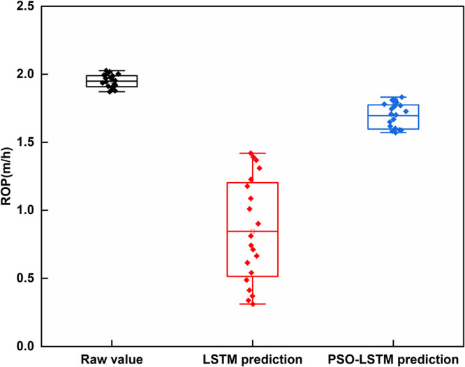
Box plot of the distribution of the raw values compared with the predicted values of the two models.
The statistical significance tests we conducted provided us with a way to assess the results of the tests. Statistical significance is an estimate of the extent to which the true data quality is within the confidence interval around the test set measurements. A commonly used level of reliability for results is 95%, also written as p = 0.05 and referred to as the p level. We added statistical significance tests for training, testing, and validation, as shown in Figure 11. The results indicate that the p value is less than 0.001, which is a very small number, indicating a good significance between the data.
Figure 11.
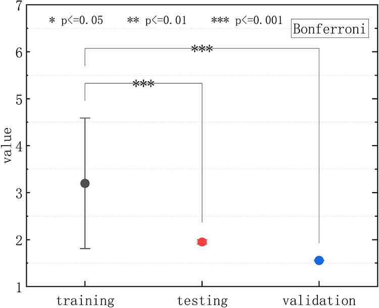
The statistical significance of the test results for training, testing, and validation.
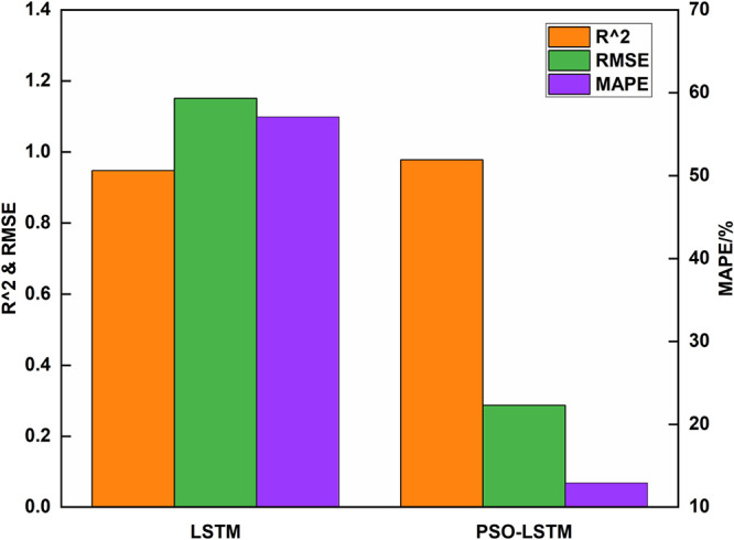
In this paper, the metrics for evaluating the performance of the model include the coefficient of determination (R2), RMSE, and mean absolute percentage error (MAPE). R2 is a statistic that measures the goodness of fit and measures the relative magnitude (i.e., percentage) of the deviation of the true value from the predicted value. The larger the value of R2 (closer to 1), the smaller the RMSE and the MAPE, indicating a better prediction performance of the model.57,58 The performance evaluation indexes of the model before and after optimization are also shown in Table 3, and the error comparison of prediction results is shown in Figures 12 and 13, where a box diagram of the accuracy before and after model optimization is presented.
Table 3. Comparison of the Model Performance Evaluation Metrics before and after Optimization.
| model type | R2 | RMSE | MAPE/% |
|---|---|---|---|
| LSTM | 0.948 | 1.151 | 57.075 |
| PSO-LSTM | 0.978 | 0.287 | 12.862 |
Figure 12.
Error comparison of LSTM model prediction results before and after optimization.
Figure 13.
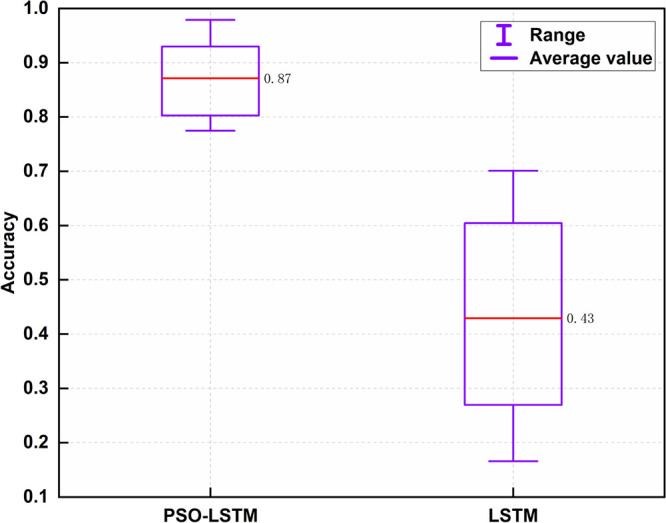
Accuracy box plot of the two models.
Table 3 and Figure 12 show that the R2 values as well as RMSE and MAPE reach 0.978, 0.287, and 12.862, respectively. Compared with the case before optimization, R2 is larger and RMSE and MAPE are smaller, indicating that the LSTM model after particle swarm optimization is more efficient. It is also seen in Figure 13 that the average accuracy of PSO-LSTM model prediction is 0.871 whereas the average accuracy of the LSTM model is 0.429. The average accuracy of the optimized LSTM model is also 44.2% higher.
5. Conclusion
This paper proposed a method of predicting ROP based on PSO and LSTM neural networks. The PSO algorithm was used to optimize the super-parameters in the construction of the LSTM model that predicts that the ROP is realized. The followings are our conclusions:
-
1.
The LSTM model optimized by the PSO algorithm converges faster, while its training time is shorter and its training efficiency is higher.
-
2.
The difference between the predicted value and the raw value of the LSTM model gradually increases with the increase of the step size, while the error of the LSTM model with PSO is reduced by increasing the step size. The RMSE of the optimized model is 0.287 less than the original value of 1.151. The predicted value of the PSO-LSTM model is also closer to the raw value, and the predicted value is more concentrated. The prediction process is also more stable, and the optimization effect of the particle swarm algorithm is much higher.
-
3.
The LSTM model optimized by particle swarm optimization R2 is 0.978, and the RMSE and MAPE values are 0.287 and 12.862, respectively. Compared with the model before optimization, R2 is larger and the RMSE and MAPE values are much smaller. These results confirm the accuracy and efficiency of the proposed model.
-
4.
The average accuracy of the LSTM model optimized by particle swarm optimization is 0.871, whereas the average accuracy of the LSTM model is 0.429; hence, the average accuracy is increased by 44.2%.
The proposed model can help the drilling engineers and decision-makers to improve drilling operation plans while shortening the drilling cycle. In the follow-up research, the author will further study the application of machine learning algorithms in various fields of petroleum and try to apply other prediction methods to the prediction of drilling parameters and full utilization of big data technology to process massive drilling data. This might result in real-time prediction, accurate prediction, and ultra-long predictions. The optimization algorithm and LSTM neural network prediction methods can expand various fields such as the actual drilling integrated design, exploration, and development, which also accelerate the realization of digitalization and intelligence.
Acknowledgments
This work was supported in part by the Major National Science and Technology projects during the 13th Five Year Plan (2016ZX05061-009), the Natural Science Foundation of Hubei Province (2018CFB770), and the COSL Science and Technology Project (G2017A-0211 T231). The authors would like to express their gratitude to EditSprings (https://www.editsprings.cn ) for the expert linguistic services provided.
The authors declare no competing financial interest.
References
- Hegde C.; Daigle H.; Gray K. E. Performance comparison of algorithms for real-time rate-of-penetration optimization in drilling using data-driven models. Spe J. 2018, 23, 1706–1722. 10.2118/191141-PA. [DOI] [Google Scholar]
- Oyedere M.; Gray K. ROP and TOB optimization using machine learning classification algorithms. J. Nat. Gas Sci. Eng. 2020, 77, 103230 10.1016/j.jngse.2020.103230. [DOI] [Google Scholar]
- Ashrafi S. B.; Anemangely M.; Sabah M.; Ameri M. J. Application of hybrid artificial neural networks for predicting rate of penetration (ROP): A case study from Marun oil field. J. Pet. Sci. Eng. 2019, 175, 604–623. 10.1016/j.petrol.2018.12.013. [DOI] [Google Scholar]
- Brenjkar E.; Delijani E. B. Computational prediction of the drilling rate of penetration (ROP): A comparison of various machine learning approaches and traditional models. J. Pet. Sci. Eng. 2022, 210, 110033 10.1016/j.petrol.2021.110033. [DOI] [Google Scholar]
- Mazen A. Z.; Rahmanian N.; Mujtaba I.; Hassanpour A. Prediction of Penetration Rate for PDC Bits Using Indices of Rock Drillability, Cuttings Removal, and Bit Wear. SPE Drill. Completion 2021, 36, 320–337. 10.2118/204231-PA. [DOI] [Google Scholar]
- Liu S.; Sun J.; Gao X.; Wang M. Analysis and establishment of drilling speed prediction model for drilling machinery based on artificial neural networks. Comput. Sci. 2019, 46, 605–608. [Google Scholar]
- Shi X.; Wang Y.; Liu Y.; Chen Y. Discussion on artificial intelligence method used in ROP prediction of drilling machinery. Petrol. Drill. Prod. Technol. 2022, 44, 105–111. [Google Scholar]
- Walker B.; Black A.; Klauber W.; Little T.; Khodaverdian M.. Roller-bit penetration rate response as a function of rock properties and well depth. In SPE Annual Technical Conference and Exhibition; OnePetro: 1986.doi: 10.2118/15620-MS. [DOI] [Google Scholar]
- Guo Y. Prediction of optimum footage and penetration rate of bit by regression analysis. Petrol. Drill. Prod. Technol. 1994, 16, 24–26. [Google Scholar]
- Mobeen M.; Mohamed M.; Zeeshan T. Experimental Investigation of a Novel, Efficient, and Sustainable Hybrid Silicate System in Oil and Gas Well Cementing. Energy Fuels 2020, 34, 7388–7396. 10.1021/acs.energyfuels.0c01001. [DOI] [Google Scholar]
- Zeeshan T.; Mobeen M.; Mohamed M. Effects of Nanoclay and Silica Flour on the Mechanical Properties of Class G Cement. ACS Omega 2020, 5, 11643–11654. 10.1021/acsomega.0c00943. [DOI] [PMC free article] [PubMed] [Google Scholar]
- Anemangely M.; Ramezanzadeh A.; Tokhmechi B. Determination of constant coefficients of Bourgoyne and Young drilling rate model using a novel evolutionary algorithm. J. Min., Environ. 2017, 8, 693–702. 10.22044/jme.2017.842. [DOI] [Google Scholar]
- Deng R.; Ma D.; Wu Z. Computer simulation of drilling process of spherical single cone bit. Pet. mach. 1999, 26, 4–6. [Google Scholar]
- Lin Y.; Shi T.; Liang Z.; Li R. Simulation study on penetration rate of percussion rotary drilling machine. J. Pet. 2004, 25, 88–92,98. [Google Scholar]
- Yan T.; Bi X.; Liu C.; Zhang S. An artificial neural network method for predicting drilling speed in deep wells. Pet. Drill. Technol. 2001, 29, 9–10. [Google Scholar]
- Amer M. M.; Dahab A. S.; El-Sayed A.-A. H.. An ROP predictive model in nile delta area using artificial neural networks. In SPE Kingdom of Saudi Arabia Annual Technical Symposium and Exhibition; OnePetro: 2017, 10.2118/187969-MS. [DOI] [Google Scholar]
- Song X.; Pei Z.; Wang P.; Zhang G.; S Y. Intelligent prediction of ROP based on support vector machine regression. Xinjiang Pet. Nat. Gas 2022, 18, 14–20. [Google Scholar]
- Ahmed O. S.; Adeniran A. A.; Samsuri A. Computational intelligence based prediction of drilling rate of penetration: A comparative study. J. Pet. Sci. Eng. 2019, 172, 1–12. 10.1016/j.petrol.2018.09.027. [DOI] [Google Scholar]
- Al-Gharbi S.; Al-Majed A.; Abdulraheem A.; Tariq Z.; Mahmoud M. Statistical Methods to Improve the Quality of Real-Time Drilling Data.ASME. J. Energy Resour. Technol. 2022, 144, 093006 10.1115/1.4053519. [DOI] [Google Scholar]
- Elkatatny S.; Tariq Z.; Mahmoud M. Real time prediction of drilling fluid rheological properties using Artificial Neural Networks visible mathematical model (white box). J. Pet. Sci. Eng. 2016, 146, 1202–1210. 10.1016/j.petrol.2016.08.021. [DOI] [Google Scholar]
- Elkatatny S.; Tariq Z.; Mahmoud M.; Abdulraheem A.; Mohamed I. An integrated approach for estimating static Young’s modulus using artificial intelligence tools. Neural Comput. Appl. 2019, 31, 4123–4135. 10.1007/s00521-018-3344-1. [DOI] [Google Scholar]
- Mmad R.; Tariq Zeeshan; Mohamed M.. Generation of Synthetic Photoelectric Log using Machine Learning Approach. Paper presented at the Abu Dhabi International Petroleum Exhibition & Conference, Abu Dhabi, UAE, November 2021, 10.2118/208201-MS. [DOI] [Google Scholar]
- Ayyaz M.; Zeeshan T.; Abdulazeez A.; Mohamed M.; Shams K.; Rizwan A. K. Shale brittleness prediction using machine learning—A Middle East basin case study. AAPG Bull. 2022, 106, 2275–2296. 10.1306/12162120181. [DOI] [Google Scholar]
- Mahmoud D.; Zeeshan T.; Murtada S. A.; Hamed A.; Mohamed M.; Dhafer A. Data-Driven Acid Fracture Conductivity Correlations Honoring Different Mineralogy and Etching Patterns. ACS Omega 2020, 5, 16919–16931. 10.1021/acsomega.0c02123. [DOI] [PMC free article] [PubMed] [Google Scholar]
- Tariq Z.; Abdulraheem A.; Mahmoud M.; Ahmed A. A Rigorous Data-Driven Approach to Predict Poisson’s Ratio of Carbonate Rocks Using a Functional Net work. Petrophys Ics 2018, 59, 761–777. 10.30632/PJV59N6-2018a2. [DOI] [Google Scholar]
- Mustafa A.; Tariq Z.; Mahmoud M. E.; Radwan A.; Abdularaheem A.; Abouelresh M. O. Data-driven machine learning approach to predict mineralogy of organic-rich shales: An example from Qusaiba Shale, Rub’al Khali Basin, Saudi Arabia. Mar. Pet. Geol. 2022, 137, 105495 10.1016/j.marpetgeo.2021.105495. [DOI] [Google Scholar]
- Anemangely M.; Ramezanzadeh A.; Tokhmechi B.; Molaghab A.; Mohammadian A. Drilling rate prediction from petrophysical logs and mud logging data using an optimized multilayer perceptron neural network. J. Geophys. Eng. 2018, 15, 1146–1159. 10.1088/1742-2140/aaac5d. [DOI] [Google Scholar]
- Bajolvand M.; Kand A. V. T.; Elmi A.; Shojaei S.; Matinkia M. Developing a New Model for Drilling Rate of Penetration Prediction Using Convolutional Neural Network. Arab. J. Sci. Eng. 2022, 47, 11953–11985. 10.1007/s13369-022-06765-x. [DOI] [Google Scholar]
- Wang J.; Cao J.; Yuan S. Shear wave velocity prediction based on adaptive particle swarm optimization optimized recurrent neural network. J. Pet. Sci. Eng. 2020, 194, 107466 10.1016/j.petrol.2020.107466. [DOI] [Google Scholar]
- Bajolvand M.; Ramezanzadeh A.; Mehrad M.; Roohi A. Optimization of controllable drilling parameters using a novel geomechanics-based workflow. J. Pet. Sci. Eng.. 2022, 218, 111004 10.1016/j.petrol.2022.111004. [DOI] [Google Scholar]
- Gan C.; Cao W.-H.; Wu M.; Chen X.; Hu Y.-L.; Liu K.-Z.; Wang F.-W.; Zhang S.-B. Prediction of drilling rate of penetration (ROP) using hybrid support vector regression: A case study on the Shennongjia area, Central China. J. Pet. Sci. Eng. 2019, 181, 106200 10.1016/j.petrol.2019.106200. [DOI] [Google Scholar]
- Wang H.; Mu L.; Shi F.; Dou H. Prediction method of oil field production in extra high water cut period based on cyclic neural network. Pet. Explor. Dev. 2020, 47, 1009–1015. [Google Scholar]
- Dong Y.; Zhang Y.; Liu F.; Cheng X. Reservoir Production Prediction Model Based on a Stacked LSTM Network and Transfer Learning. ACS Omega 2021, 6, 34700–34711. 10.1021/acsomega.1c05132. [DOI] [PMC free article] [PubMed] [Google Scholar]
- Chang Z.; Zhang Y.; Chen W. Electricity price prediction based on hybrid model of adam optimized LSTM neural network and wavelet transform. Energy 2019, 187, 115804. 10.1016/j.energy.2019.07.134. [DOI] [Google Scholar]
- Kim Y. D.; Durlofsky L. J. A recurrent neural network–based proxy model for well-control optimization with nonlinear output constraints. SPE J. 2021, 26, 1837–1857. 10.2118/203980-PA. [DOI] [Google Scholar]
- Yin Q.; Yang J.; Tyagi M.; Zhou X.; Hou X.; Wang N.; Tong G.; Cao B. Machine learning for deepwater drilling: Gas-kick-alarm Classification using pilot-scale rig data with combined surface-riser-downhole monitoring. SPE J. 2021, 26, 1773–1799. 10.2118/205365-PA. [DOI] [Google Scholar]
- Hou L.; Cheng Y.; Elsworth D.; Hong L. H. J. Prediction of the Continuous Probability of Sand Screen out Based on a Deep Learning Workflow. SPE J. 2022, 27, 1520–1530. 10.2118/209192-PA. [DOI] [Google Scholar]
- Hu Z. Crude oil price prediction using CEEMDAN and LSTM-attention with news sentiment index. Oil & Gas Science and Technology–Revue d’IFP Energies nouvelles 2021, 76, 28. 10.2516/ogst/2021010. [DOI] [Google Scholar]
- Shi J.; Al-Durra A.; Matraji I.; Al-Wahedi K.; Abou-Khousa M. Application of Particle Swarm Optimization (PSO) algorithm for Black Powder (BP) source identification in gas pipeline network based on 1-D model. Oil & Gas Science and Technology–Revue d’IFP Energies nouvelles 2019, 74, 47. 10.2516/ogst/2019016. [DOI] [Google Scholar]
- Xu C.; Liu B.; Liu K.; Guo J. Intelligent model for landslide displacement time series analysis and prediction based on particle swarm Gaussian process regression coupling algorithm. Geotech. Mech. 2011, 32, 1669–1675. [Google Scholar]
- Huang S.; Tian L.; Zhang J.; Chai X.; Wang H.; Zhang H. Support Vector Regression Based on the Particle Swarm Optimization Algorithm for Tight Oil Recovery Prediction. ACS Omega 2021, 6, 32142–32150. 10.1021/acsomega.1c04923. [DOI] [PMC free article] [PubMed] [Google Scholar]
- Wu S. B.; Chen Z. G.; Huang R. ID3 optimization algorithm based on correlation coefficient. Comp. Eng. Sci. 2016, 38, 2342–2347. [Google Scholar]
- Rui J. H.; Chen J. W.; Bao H. W.; Jian Y.; Xin X.; Su W. W.; Su Q. H. Well performance prediction based on Long Short-Term Memory (LSTM) neural network. J. Pet. Sci. Eng. 2022, 208, 109686. [Google Scholar]
- Hochreiter S.; Schmidhuber J. Flat minima. Neural Comput. 1997, 9, 1–42. 10.1162/neco.1997.9.1.1. [DOI] [PubMed] [Google Scholar]
- Xu K.; Shen X.; Yao T.; Tian X.; Mei T.. Greedy layer-wise training of long short term memory networks. In 2018 IEEE International Conference on Multimedia & Expo Workshops (ICMEW); IEEE: 2018; pp. 1–6.
- Ao L.; Pang H.. Prediction of POR Based on Artificial Neural Network with Long and Short Memory (LSTM). In 55th US Rock Mechanics/Geomechanics Symposium; OnePetro: 2021. [Google Scholar]
- Kennedy J.; Eberhart R.. Particle swarm optimization. In Proceedings of ICNN’95-international conference on neural networks; IEEE: 1995; pp. 1942–1948.
- Huo F.; Chen Y.; Ren W.; Dong H.; Yu T.; Zhang J. Prediction of reservoir key parameters in ‘sweet spot’on the basis of particle swarm optimization to TCN-LSTM network. J. Pet. Sci. Eng. 2022, 214, 110544 10.1016/j.petrol.2022.110544. [DOI] [Google Scholar]
- Zhou C.; Gao H.; Gao G.; Zhang W. Particle swarm optimization. Comp. Appl. Res. 2003, 20, 7–11. [Google Scholar]
- Li W.; Xu Q.; Kong D.; Zhang X.; Gu Y.; Lv Y. Joint operation optimization model of SCR denitration system for power station boilers. Thermal power generation 2019, 48, 46–52. [Google Scholar]
- Aguila-Leon J.; Vargas-Salgado C.; Chiñas-Palacios C.; Díaz-Bello D. Energy management model for a standalone hybrid microgrid through a particle Swarm optimization and artificial neural networks approach. Energy Convers. Manage. 2022, 267, 115920 10.1016/j.enconman.2022.115920. [DOI] [Google Scholar]
- Xue L.; Gu S.; Wang J.; Liu Y.; Tu B. Prediction of gas well production performance based on particle swarm optimization and short-term memory neural network. Petrol. Drill. Prod. Technol. 2021, 43, 525–531. [Google Scholar]
- Wang X.; Deng W.; Qi W. Short term power load forecasting model based on hyperparametric optimization. Foreign electronic measurement technology 2022, 41, 152–158. [Google Scholar]
- Pan S.; Wang C.; Zhang Y.; Cai W. Lithologic identification based on long-term and short-term memory neural network to complete logging curve and hybrid optimization xgboost. Journal of China University of Petroleum (NATURAL SCIENCE EDITION) 2022, 46, 62–71. [Google Scholar]
- Kim J.; Park J.; Shin S.; Lee Y.; Min K.; Lee S.; Kim M. Prediction of engine NOx for virtual sensor using deep neural network and genetic algorithm. Oil & Gas Science and Technology–Revue d’IFP Energies nouvelles 2021, 76, 72. 10.2516/ogst/2021054. [DOI] [Google Scholar]
- Guevara J.; Zadrozny B.; Buoro A.; Lu L.; Tolle J.; Limbeck J. W.; Hohl D. A machine-learning methodology using domain-knowledge constraints for well-data integration and well-production prediction. SPE Reservoir Eval. Eng. 2019, 22, 1185–1200. 10.2118/195690-PA. [DOI] [Google Scholar]
- Alalimi A.; Pan L.; Al-Qaness M. A.; Ewees A. A.; Wang X.; Abd Elaziz M. Optimized Random Vector Functional Link network to predict oil production from Tahe oil field in China. Oil & Gas Science and Technology–Revue d’IFP Energies nouvelles 2021, 76, 3. 10.2516/ogst/2020081. [DOI] [Google Scholar]
- Temizel C.; Canbaz C. H.; Saracoglu O.; Putra D.; Baser A.; Erfando T.; Krishna S.; Saputelli L.. Production forecasting in shale reservoirs through conventional DCA and machine/deep learning methods. In Unconventional Resources Technology Conference, 20–22 July 2020; Unconventional Resources Technology Conference (URTeC): 2020; pp. 4843–4894, 10.15530/urtec-2020-2878. [DOI] [Google Scholar]