Finite Element Analysis of Bone Mechanical Properties using MRI-derived Bound and Pore Water Concentration Maps

Abstract

Ultrashort echo time (UTE) MRI techniques can be used to image the concentration of water in bones. Particularly, quantitative MRI imaging of collagen-bound water concentration (C_bw) and pore water concentration (C_pw) in cortical bone have been shown as potential biomarkers for bone fracture risk. To investigate the effect of C_bw and C_pw on the evaluation of bone mechanical properties, MRI-based finite element models of cadaver radii were generated with tissue material properties derived from 3D maps of C_bw and C_pw measurements. Three-point bending tests were simulated by means of the finite element method to predict bending properties of the bone and the results were compared with those from direct mechanical testing. The study results demonstrate that these MRI-derived measures of C_bw and C_pw improve the prediction of bone mechanical properties in cadaver radii and have the potential to be useful in assessing patient-specific bone fragility risk.

Introduction

Bone fragility is a widespread problem and current X-ray based diagnostics have not proven effective in predicting who is likely to suffer a fragility fracture (Cosman et al. 2014; Kanis et al. 2001). Magnetic resonance imaging (MRI) has shown promise to provide complimentary diagnostics of bone fracture risk (Manhard et al. 2017b). In cortical bone, MRI can measure concentrations water bound to collagen (bound water concentration, C_bw) and water inside pore spaces (pore water concentration, C_pw), and these two measures have been shown to correlate with various mechanical properties of cadaveric bone specimens (Horch et al. 2011) and whole bones (Manhard et al. 2016). This study aimed to determine whether MRI-derived C_bw and C_pw information can improve the prediction of mechanical bone properties, beyond what can be determined by structure alone. To this end, finite element (FE) analysis was used to incorporate MRI measurements of C_bw and C_pw along with the bone structure into the evaluation of whole cadaver bone mechanical properties.

Materials and Methods

Thirty-five fresh, frozen cadaveric forearms (elbow to fingertip, N_b = 35) from 29 donors (14 males, 15 females, age 57 to 84, mean 72 ± 8, right and left pairs came from the 6 donors) were obtained from the United Tissue Network (Phoenix, AZ, USA). Each arm was studied using three measurements. First, 3D MRI provided structure and maps of C_bw and C_pw of the cortical region of the radius. Second, mechanical properties of the radius were measured with a three-point bending test. Finally, using MRI to define structure and material properties, FE simulations of the 3-point bending test were performed with the objective of evaluating how C_bw and C_pw relate to whole bone mechanics. Figure 1 presents a summary of the overall experimental plan, and details of each phase of the study are presented below.

Figure 1.

The experiment overview. For the ith bone, i = 1 to N_b, material properties, Ei and Yi, were iteratively adjusted until the root mean square difference between the simulated and experimentally measured force-displacement curves was minimized.

Imaging

After thawing, MRI of each arm was acquired on a Philips Intera Achieva (Best, NL) 3 T scanner using a dStream Flex-M coil for signal reception and the body coil for RF transmission. Similar to previous work, an adiabatic inversion recovery (AIR) prepared ultra-short echo time (UTE) sequence was used to selectively image bound water, and a double adiabatic inversion recovery (DAFP) prepared UTE sequence was used for selective imaging of pore water (Horch et al. 2012; Manhard et al. 2013). All images were acquired with a 3D radial readout to encode a 20 cm × 20 cm × 20 cm field-of-view (FOV) with 1 mm nominal isotropic resolution. The AIR sequence used a 7.8 ms duration, 3.2 kHz bandwidth HS8 adiabatic inversion pulse, inversion time = 85 ms, and a repetition time (T_R) = 400 ms. The DAFP sequence used a pair of the same adiabatic pulses and T_R = 615 ms. Both AIR and DAFP acquisitions were accelerated by acquiring 16 radial spokes in k-space per repetition, using 115-μs duration hard pulse RF excitations with variable flip angle to generate an equal amplitude of transverse magnetization (initial angle = 12.5° and net effective flip angle = 60°). Conventional 3D UTE images were also acquired for anatomical reference of the bone with T_R = 4.8 ms, 70 μs echo time, and a 7° flip angle excitation pulse.

Similar to previous studies (Manhard et al. 2016; Manhard et al. 2017a), UTE images were reconstructed (Johnson and Pipe 2009) based upon measured readout gradient trajectories (Duyn et al. 1998; Harkins et al. 2021), and image intensities were adjusted to account for the receive coil spatial sensitivity (Duyn et al. 1998; Fessler and Sutton 2003). After image reconstruction, C_bw and C_pw maps were calculated using previously presented signal equations (Manhard et al. 2013). These maps were computed in absolute units of concentration (moles of ¹H per liter of bone) using signal a reference phantom (10% CuSO₄ + H₂O/90% D₂O), which was included in the FOV. For each bone, the conventional UTE MRI was used to generate a 3D mask of cortical bone, 110 mm in length and centered on the distal-third site. Mean C_bw and C_pw values, (${\stackrel{\mathrm{-}}{C}}_{\text{bw}}$ and ${\stackrel{\mathrm{-}}{C}}_{\text{pw}}$, respectively) were computed from within the mask at the central axial slice.

Mechanical testing

Following MRI, the radii were denuded and subjected to a three-point bending test with a material testing machine (MTS 858 Bionix, Eden Prairie, MN). The distal-third radius site, approximately the middle of the MRI FOV, was loaded at 6.5 mm/min until failure. Each bone was positioned with the anterior surface down and the medial side forward with the span supports equal to 98 mm. The resulting force and displacement data were recorded at 100 Hz with a 14.5 kN load cell and an MTS linear variable displacement transducer, respectively. From the force-displacement data, stiffness, yield force, pre-yield work, and work-to-fracture were calculated, and indicated in Figure 2.

Figure 2.

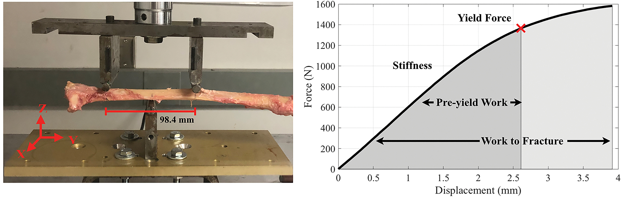
Three-point bending test setup (left) and force-displacement curve of a representative radius. From the force-displacement data, stiffness, yield force (15% loss in stiffness), pre-yield work (area under the force-vs.-displacement curve until the yield point), and work-to-fracture (area under the force-vs.- displacement curve until the failure point) were calculated (Manhard et al. 2016). Failure was defined as 5% decrease from the ultimate force.

FE Analysis

Using the 3D bone mask from the UTE MRI and TetGen (Si H. 2015), a first-order tetrahedral mesh of each bone was generated with elemental volume of 0.118 mm³ (i.e., edge length ≈ 1 mm, matching MRI resolution). With this mesh and using FEBioStudio (Maas et al. 2012) and the GIBBON toolbox (Moerman 2018), an FE model was used to simulate the same three-point bending mechanical test described above. The material behavior of bone was implemented with an elastic, perfectly plastic stress-strain model, as defined in the FEBioStudio software. (The material is perfectly elastic until a certain stress and then becomes perfectly plastic, i.e., no addition stress with additional strain.) The elastic regime was defined as isotropic and linear with Young’s modulus (E) and Poisson ratio of 0.3. The onset of the perfectly plastic regime was defined by the von Mises yield stress (Y).

From the simulation, the resulting force, displacement, stress, and strain were recorded at a minimum of twenty time-steps for each node. The global force-displacement data were then generated using the summation of reaction force data from the nodes at which the loading was applied. For each bone, the global force-displacement data from the simulation and mechanical tests were compared from the start of loading until failure point, defined as the mean von Mises equivalent strain along the maximum loading plane exceeding 3%. With this failure criterion, the simulations predicted a failure displacement between the experimental yield displacement and fracture displacement. The experimental and simulated forces were linearly interpolated to a uniformly spaced array of 100 points between the start of loading and ultimate force, and then the root mean square difference between the two was computed (δ).

Within this framework, simulations were repeated until values for E and Y were found that minimized δ, resulting in per-bone estimated material property values, ${\widehat{E}}_i$ and ${\widehat{Y}}_i$, for i = 1 to N_b. This was done with a Nelder-Mead simplex search, using initial values of E = 9 GPa and Y = 200 MPa. Across all bones, the minimization was completed in 18 to 41 iterations. In addition, simultaneous simulations across all bones were repeated until a global solution of E and Y were found that minimized the sum of δ from all N_b bones. These values were labeled E_A and Y_A and were used on Case A evaluations—see definition below.

Predicting Mechanical Properties with MRI

First, linear models were defined that related MRI measures of mean bound and pore water concentrations (${\stackrel{\mathrm{-}}{C}}_{\text{bw}}$ and ${\stackrel{\mathrm{-}}{C}}_{\text{pw}}$, respectively) to the estimated bone material properties, modulus ($\widehat{E}$) and yield stress ($\widehat{Y}$),

$${\widehat{E}}_i=a_1{\overline{C}}_{\text{bw},i}+a_2{\overline{C}}_{\text{pw},i}+a_3$$ (1)

$${\widehat{Y}}_i=b_1{\overline{C}}_{\text{bw},i}+b_2{\overline{C}}_{\text{pw},i}+b_3,$$ (2)

with i = 1 to N_b. These models were using standard linear regression, providing estimated parameters, ${\widehat{a}}_1-{\widehat{a}}_3$ and ${\widehat{b}}_1-{\widehat{b}}_3,$ which were subsequently used in cases B and C, below. Second, to test the influences of C_bw and C_pw in predicting whole-bone mechanical test results, the FE simulations were repeated using three different cases to define modulus, E, and yield stress, Y. For each case, the simulated force-displacement curves were used to estimate predicted mechanical properties: stiffness, yield force, and pre-yield work, and work to fracture, as described above. The three cases evaluated were:

1. No influence of C_bw and C_pw. The modulus and yield stress were spatially homogenous and constant across bones, using the globally optimal parameters, E_A and Y_A.

2. Homogeneous influence of C_bw and C_pw. The modulus and yield stress were defined as spatially homogeneous but unique to each bone, based on ${\stackrel{\mathrm{-}}{C}}_{\text{bw}}$ and ${\stackrel{\mathrm{-}}{C}}_{\text{pw}}$. Thus, for the i^th bone, case B modulus and yield stress were:

   $$E_{\text{B},i}={\widehat{a}}_1{\overline{C}}_{\text{bw},i}+{\widehat{a}}_2{\overline{C}}_{\text{pw},i}+{\widehat{a}}_3$$ (3)

   $$Y_{\text{B},i}={\widehat{b}}_1{\overline{C}}_{\text{bw},i}+{\widehat{b}}_2{\overline{C}}_{\text{pw},i}+{\widehat{b}}_3,$$ (4)

   respectively.
3. Heterogeneous influence of C_bw and C_pw. The modulus and yield stress were defined as spatially varying maps, based on the C_bw and C_pw maps. Thus, for every FE element of the i^th bone, case C modulus and yield stress were:

   $$E_{\mathrm{C},i}={\widehat{a}}_1{C}_{\text{bw},i}+{\widehat{a}}_2{C}_{\text{pw},i}+{\widehat{a}}_3$$ (5)

   $$Y_{\mathrm{C},i}={\widehat{b}}_1{C}_{\text{bw},i}+{\widehat{b}}_2{C}_{\text{pw},i}+{\widehat{b}}_3,$$ (6)

   respectively.

Results

From a representative cadaver arm, cross-sectional UTE, AIR, and DAFP MRI images at the distal-third site are shown in Figure 3. The UTE image (left) was cropped to show the cross-sectional image of the arm and the red box indicates the location of the radius bone. Maps of C_bw and C_pw within the radius are overlaid on the corresponding AIR and DAFP images, respectively. Across all 35 bones, the median ± standard deviation of the mean C_bw and C_pw, calculated at middle slice, were 15.37 ± 4.22 ¹H mol/L_bone and 14.98 ± 9.34 ¹H mol/L_bone, respectively.

Figure 3.

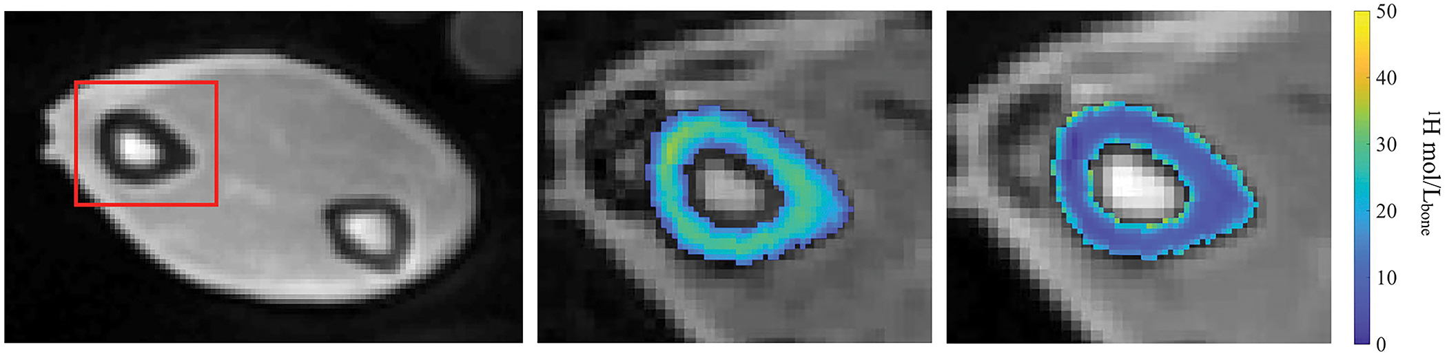
MRI images of a representative radius acquired at distal third site. The left image shows the conventional UTE image with red box indicating the radius bone. The middle and right images show the maps of C_bw and C_pw overlaid on the corresponding AIR and DAFP images, respectively.

The results of the simulation-derived per-bone estimates of modulus, $\widehat{E}$, and yield stress, $\widehat{Y}$, are shown in Figure 4 for two representative bones. Each frame shows the experimental force-vs.-displacement curve (black) as well as the simulation-derived curves generated using the per-bone (blue) and global (orange) estimates of elastic modulus and yield stress. In all cases, the spatially-uniform, per-bone optimized $\widehat{E}$ and $\widehat{Y}$ values resulted in simulated force-displacement curves that closely matched the experimental results with average coefficient of determination, R² ≈ 0.99 across all samples. The mean ± standard deviation (range) of the estimated $\widehat{E}$ and $\widehat{Y}$ were 9.42 ± 2.13 GPa (5.26 to 14.48 GPa) and 140.72 ± 34.93 MPa (60.87 to 226.97 MPa), respectively. The globally-optimized elastic modulus and yield stress values, E_A = 8.66 GPa and Y_A = 131.88 MPa, respectively (11 iterations), resulted in simulated force-vs.-displacement curves that were qualitatively similar to experimental data with average coefficient of determination, R² ≈ 0.60. These E_A and Y_A values were used for the case A evaluations.

Figure 4.

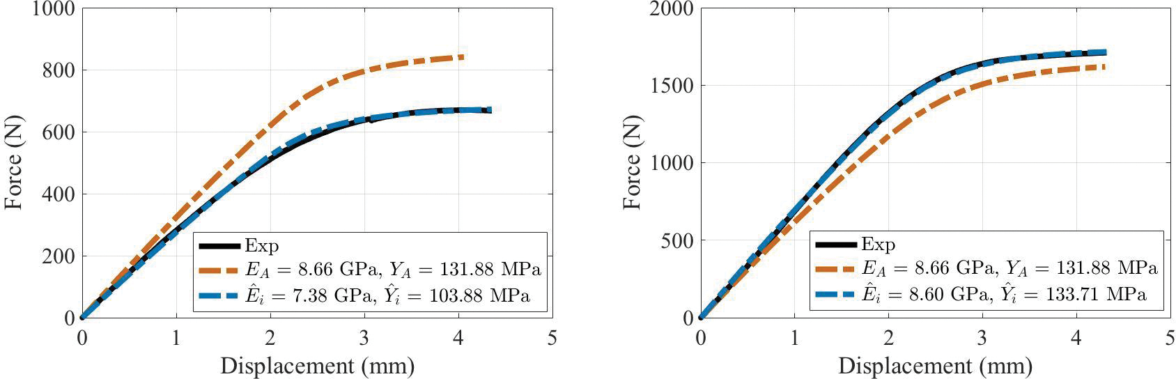
Experimental (solid line) and simulated (dashed line) force-displacement curves using $\{{\widehat{E}}_i,{\widehat{Y}}_i\}$ (blue) and {E_A, Y_A} (orange) parameters from two representative bones.

The linear models relating imaging measures, ${\stackrel{\mathrm{-}}{C}}_{\text{bw},i}$ and ${\stackrel{\mathrm{-}}{C}}_{\text{pw},i}$, to ${\widehat{E}}_i$ and ${\widehat{Y}}_i$ (Eqs 1 and 2) are shown in Figure 5. These models were primarily driven by bound water concentrations and captured approximately half of the variance of ${\widehat{E}}_i$ and ${\widehat{Y}}_i$ (coefficient of determination, R² = 0.47 and 0.60, for the models predicting modulus and yield stress, respectively). The fitted model parameters, ${\widehat{a}}_1-{\widehat{a}}_3$ and ${\widehat{b}}_1-{\widehat{b}}_3$ are presented in Table 1 and were used to define material properties E_B, Y_B, and maps E_C and Y_C, for the case B and C evaluations, below.

Figure 5.

Correlations of elastic modulus (left) and yield stress (right) with MRI-derived C_bw and C_pw.

Table 1:

Parameters estimation for multiple linear regression model between water concentration measurements and optimized tissue parameters.

Properties	Coefficient (Variables)	Estimate (Mean ± SE) (Units)	R2
Young’s Modulus (GPa)	a1 (Cbw)	0.39 ± 0.08 (GPa∙Lbone/mol 1H)	0.47
	a2 (Cpw)	0.05 ± 0.04 (GPa∙Lbone/mol 1H)
	a3 (Intercept)	2.06 ± 1.88 (GPa)
Yield Strength (MPa)	b1 (Cbw)	6.60 ± 1.17 (GPa Lbone/mol 1H)	0.60
	b2 (Cpw)	0.15 ± 0.53 (GPa∙Lbone/mol 1H)
	b3 (Intercept)	29.71 ± 26.74 (MPa)

The three cases of simulations are compared in Figures 6 and 7 and Table 2. First, from two representative bones, Figure 6 shows the comparison between experimental force-displacement curve and the simulated curves from cases A, B, and C. Note that in Case C, 4 of the bone models failed to converge at high displacement but were successfully re-run using a neo-hookean nonlinear model (within FEBioStudio) in place of the isotropic elastic model. Subsequent analysis below is reported with and without inclusion of these four simulations.

Figure 6.

Experimental (solid line) and model-based (dashed line) simulated force-displacement curves from case A (orange), case B (green), and case C (blue) of two representative bones.

Figure 7.

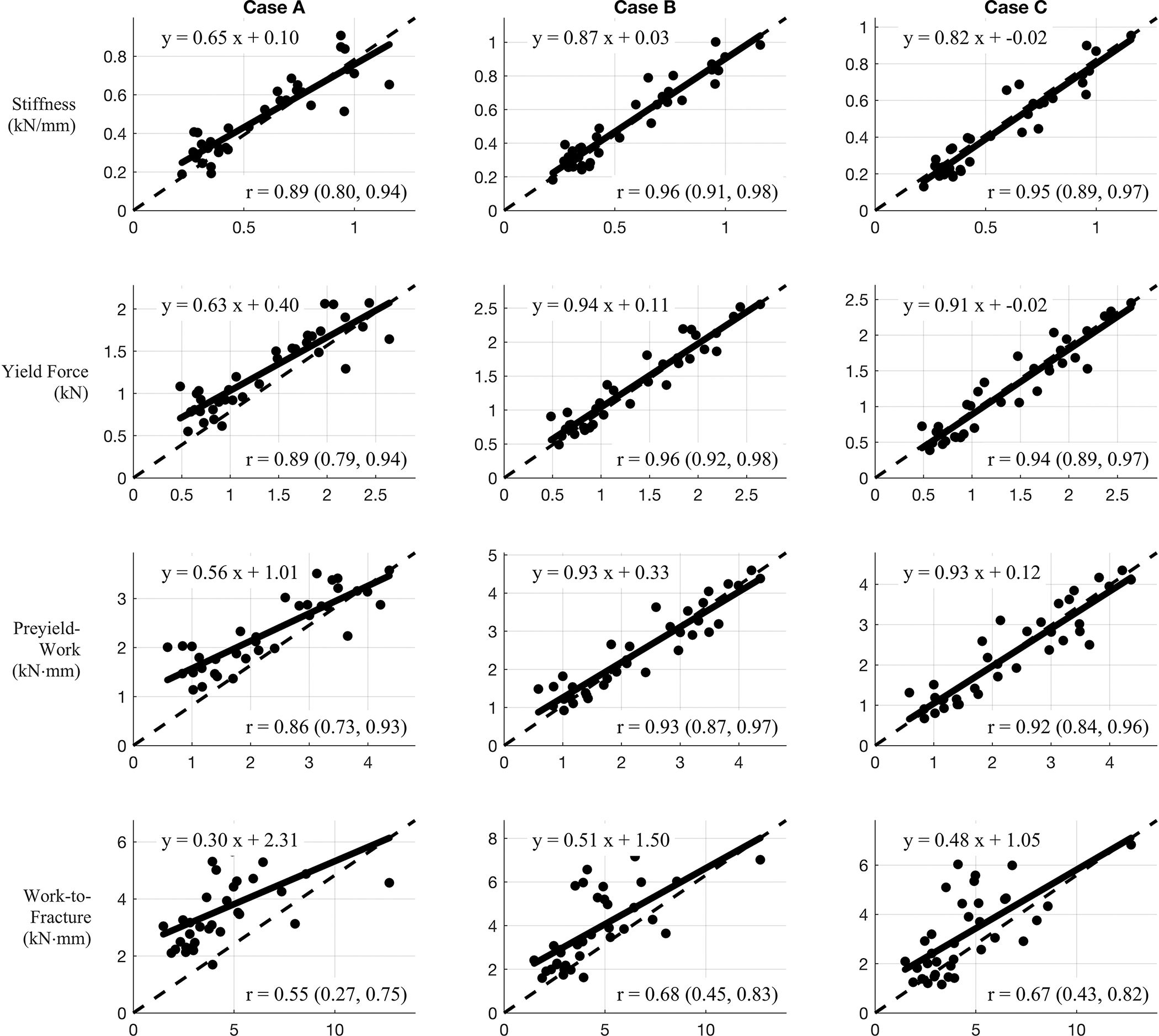
Correlations between measured mechanical data (x-axis) and predicted mechanical data (y-axis) of three different models. Case A: Homogeneous tissue properties, Case B: Homogeneous tissue properties derived from C_bw and C_pw, and Case C: Heterogeneous tissue properties derived from C_bw and C_pw.

Table 2:

Linear model and correlation coefficients of mechanical properties between mechanical data and simulation data for three different models.

Properties	Case	Linear Model Coefficients (with 95% confidence bounds)		Correlation Coefficient (with 95% confidence bounds)
		Slope	Intercept
Stiffness (kN/m)	A	0.65 (0.56, 0.75)	0.10 (0.04, 0.17)	0.89 (0.80, 0.94)
	B	0.87 (0.79, 0.95)	0.03 (−0.02, 0.08)	0.96 (0.91, 0.98)
	C	0.82 (0.74, 0.91)	− 0.02 (−0.07, 0.03)	0.95 (0.89, 0.97)
Yield Force (kN)	A	0.63 (0.54, 0.73)	0.40 (0.26, 0.54)	0.89 (0.79, 0.94)
	B	0.94 (0.85, 1.02)	0.11 (−0.02, 0.23)	0.96 (0.92, 0.98)
	C	0.91 (0.82, 1.01)	− 0.02 (−0.16, 0.12)	0.94 (0.89, 0.97)
Pre-yield Work (kNmm)	A	0.56 (0.46, 0.66)	1.01 (0.76, 1.26)	0.86 (0.73, 0.93)
	B	0.93 (0.82, 1.03)	0.33 (−0.07, 0.60)	0.93 (0.87, 0.97)
	C	0.93 (0.81, 1.04)	0.12 (−0.18, 0.42)	0.92 (0.84, 0.96)
Work to Fracture (kNmm)	A	0.30 (0.17, 0.44)	2.31 (1.63, 2.99)	0.55 (0.27, 0.75)
	B	0.51 (0.35, 0.67)	1.50 (0.69, 2.31)	0.68 (0.45, 0.83)
	C	0.48 (0.32, 0.63)	1.05 (0.27, 1.83)	0.67 (0.43, 0.82)

In terms of the four bending properties derived from the force-displacement data, Figure 7 displays the correlations between bending properties from mechanical testing and simulation for the three different cases. Case B and C displayed stronger prediction power for all evaluated bone mechanical properties in comparison to case A. Each frame reports a linear model along with a correlation coefficient (r) (with 95% confidence interval, CI) between predicted (from simulation) and measured bending property. These values along with the CI of the model parameters are summarized in Table 2. In almost all cases, the inclusion of bound and pore water concentrations (cases B and C) resulted in better prediction of measured properties than did predictions based on bone structure alone. Specifically, for all bending properties, the model slope and intercept parameters were closer to unity and zero, respectively, for cases B and C compared to case A. Similarly, the case B and C correlation coefficients were higher than those from case A, although the CIs overlapped in all comparisons. If we exclude the 4 Case C simulations that required the neo-hookean model, none of the correlation coefficients changed by more than 0.02.

Discussion

Image-based FE methods have been used in multiple studies together with computed tomography (Kopperdahl et al. 2014; Ladd et al. 1998; Ramezanzadehkoldeh and Skallerud 2017), or MRI data (Chang et al. 2014; Newitt et al. 2002; Rajapakse et al. 2018; Zhang et al. 2013) to predict bone strength. For MRI studies, material properties were typically either assumed as homogeneous (E = 10 GPa) (Newitt et al. 2002), derived from bone volume fraction which requires high-resolution μMRI imaging (E = 15 GPa × BV/TV) (Chang et al. 2014; Rajapakse et al. 2018), or defined as a function of tissue strain (hyperbolic secant of ε_tissue × 15 GPa) (Zhang et al. 2013). Also, only one study compared FE predictions to experimental measurements, namely compression tests of distal tibia segments (Rajapakse et al. 2018). In the present study, FE simulations derived from MRI images used material properties encoded with matrix and micro-structural information to simulate force-displacement curves of whole radii subjected load-to-failure tests in three-point bending. In doing so, FE predictions of bone strength from MRI scans can be based on both images of structure and material characteristics, namely bound and pore water concentrations, akin to QCT-based FE predictions of bone strength that incorporate relationships between modulus or yield stress and calibrated X-ray attenuation values (Knowles et al. 2016).

Using only anatomical information from MRI and assuming Poisson’s ratio = 0.3, the elastic material properties, modulus and yield stress, were found that resulted in the best prediction of the mechanical tests. These values varied widely across the 35 bones tested (ranges: $\widehat{E}$ = 5.26 to 14.48 GPa and $\widehat{Y}$ = 60.87 to 226.97 MPa) but are in reasonable agreement literature values for cortical bone (11.5 GPa elastic modulus and 114 MPa yield stress (Reilly and Burstein 1975). Measurements specific to whole bone bending properties of the human radius are scarce but are also generally similar. For example, Singh et al. reported mean and standard deviation of elastic modulus and strength from 6 cadaver radii as 3.66 ± 0.78 GPa and 80.31 ± 14.55 MPa, respectively (Singh et al. 2018). This same study also cited bending modulus and strength values of the radial diaphysis from Motoshima (Motoshima 1960) as 15.88 GPa elastic modulus and 211.82 ± 4.9 MPa strength. Thus, the optimal values of modulus and yield stress are in good general agreement with values reported for the radius.

Importantly, the results showed that when using optimal per-bone values, ${\widehat{E}}_i$ and ${\widehat{Y}}_i$, the FE simulations closely predicted force-displacement curves of mechanical tests (R² ≈ 0.99 across all bones). The coefficient of determination dropped by nearly half (R² = 0.60) when using the globally optimized values (E_A = 8.66 GPa and Y_A =131.88 MPa) for all simulations. This observation indicates that, in addition to macroscopic structure, donor-specific bone material properties were important in determining the whole bone bending behavior (i.e., force vs. displacement). Given this, the subsequent FE simulations were used to determine if these material properties could be derived from MRI measures of bone and pore water concentration.

Our previous studies suggested positive and negative associations between both C_bw and C_pw, respectively, and various mechanical properties of cortical bone as determined by load-to-failure tests of uniform specimens (Granke et al. 2015; Horch et al. 2011). Horch et al. presented relatively strong linear correlations between bound- and pore- water ¹H NMR concentrations and flexural modulus and yield stress (Horch et al. 2011). In our subsequent MRI study of cadaveric radii, C_bw and C_pw measurements also showed significant and independent linear relationship with bone bending strength (Manhard et al. 2016). For that study, material properties of whole bone radius, such as bending strength and toughness, were determined using beam theory and μCT-derived section modulus. Consequently, a linear model was chosen to relate these MRI measures to elastic modulus and yield stress (Equations 1 and 2, respectively). Overall, the models captured approximately half of the variance in ${\widehat{E}}_i$ and ${\widehat{Y}}_i$ across bones and demonstrated that both modulus and strength are strongly dependent on C_bw (see fitted models in Figure 5 and fitted parameters in Table 1). These linear models were then used to compute per-bone values E_B,i and Y_B,i, as well as per-bone maps E_C,i and Y_C,i for repeated FE simulations.

The contribution of pore water concentration to E and Y was low despite the range in C_pw being greater in the present set of cadaveric radii than in our previous study (Manhard et al. 2016). There are several possible explanations for this weak contribution of C_pw to the material properties of cortical bone. Firstly, our previous study in which both C_pw and C_bw significantly contributed to the prediction of bending strength of the radial diaphysis did not use FEA to account for role of bone structure in strength. By accounting for size and shape of each bone in the FE simulations, the importance of C_pw was perhaps diminished. Secondly, although cortical porosity is a known determinant of bone strength (Curry 1990; McCalden et al. 1993; Wachter et al. 2002), its negative correlation with yield stress has been shown to be rather weak (e.g., R² = 0.22, p=0.004) (Mirzaali et al. 2016). Lastly, higher pore water concentration (higher cortical porosity) does not necessarily translate to weaker bone if the C_pw is dictated by signal from the endosteum. Bone loss in the diaphysis of long bones occurs near the endosteum causing a “transition” zone in which cortical bone appears to be trabecular bone (Zebaze et al. 2010). Loading cadaveric radii in four-point bending to failure and imaging the micro-structure of the diaphysis by high-resolution μCT, Bigelow et al. observed a stronger correlation between pores distributed away from the neutral axis and bending strength than between overall porosity and bending strength (Bigelow et al. 2019). Since the imaging resolution of this study is 1 mm, high C_pw values could also be influenced by bone marrow signal in the endosteum region, especially for bones with a thin cortical shell. The literature values of mean cortical thickness of radius bones (2.51 $\pm$ 0.58 mm (Louis et al. 1995) and 5.75 $\pm$ 1.07 mm (Webber et al. 2015) also shown that cortical thickness for some bone samples could be relatively close to the imaging resolution. This effect would be smaller in C_bw measurements since bone marrow signals are suppressed in the AIR pulse sequence.

The potential for MRI measures of bound and pore water concentration to inform on the bending properties of bone was assessed by comparing results of three sets of FE simulations. Rather than simply computing the mean squared difference in the force-displacement curves between experiment and simulation, these evaluations compared four bending properties that were computed from the force-displacement data. The results across all cases for defining material properties and all four bending properties are summarized in Figure 7.

Using only structural information from MRI (Case A), the simulations predicted the experimentally measured bending properties well, with correlation coefficient values ranging 0.55 to 0.89. However, this level of predictive power required the use of optimal values of modulus and yield stress found for this particular collection of cadaver bones. Had these simulations relied on literature values, as has been done for some previous FE simulations (Newitt et al. 2002), the predictive power of the simulations would have been much lower. Using the MRI measures of C_bw and C_pw to define the bone material properties (Cases B and C) resulted in generally better prediction of bending properties by simulation. These improved predictions were reflected in both increased correlation coefficient values and models closer to the line of identity. The 95% confidence intervals of the slope and intercept included the values of 1 and 0, respectively, in stiffness for cases B and C (Table 2). The added value of MRI measures was particularly true for the one post-yield property (work-to-fracture) as the correlation coefficient values was increased by up to 23 percent. This may reflect the role of collagen and collagen hydration status in the ability of bone to resist crack propagation.

In comparing Cases B (homogeneous E and Y) and C (inhomogeneous E and Y), there was little or no improvement in predictive power. This result is not surprising, given that a uniform modulus and yield stress optimized for each bone (${\widehat{E}}_i$ and ${\widehat{Y}}_i$) resulted in FE simulations that nearly perfectly predicted experimental force-displacement curves. Nonetheless, there were some differences in results between the results of Cases B and C. The bending properties predicted by Case B were generally higher than those from Case C, as apparent from the intercept terms and position of best fit lines relatively to the identity line (Figure 7). These subtle differences are consistent with one previous study of cancellous bone, which found an overestimation of elastic stiffness tensor with a homogeneous model but a generally minor influence of mineral heterogeneity (Gross et al. 2012).

Also, the comparison between Cases B and C may have been limited by the use of mean C_bw and C_pw values in establishing the material model linearly relating E and Y to these MR-derived characteristics. Ideally, the model parameters a₁, a₂, a₃ and b₁, b₂, b₃ could be estimated directly from iterative joint FE simulations of all bones, as was done to find E_A and Y_A. However, the time required for such a computation made it infeasible. To our knowledge, no study has tested the effect of tissue modulus variation on the whole bone modulus and strength of cortical bone; however, apparent modulus of trabecular bone has been found to decrease nonlinearly with increasing coefficient of variation of intra-or-within-specimen tissue modulus (Jaasma et al. 2002). Moreover, several studies have presented the importance of the composition, distribution, and architecture of lamellar tissue in reproducing the micromechanical failure mode of trabecular bone (Hammond et al. 2019; Hammond et al. 2018; Torres et al. 2016; Renders et al. 2008). If the heterogeneity in actual material properties (tissue-level modulus) significantly affects whole bone bending properties, then the estimated ${\widehat{a}}_1,{\widehat{a}}_2,{\widehat{a}}_3$ and ${\widehat{b}}_1,{\widehat{b}}_2,{\widehat{b}}_3$ would not be an accurate representation for calculating E_C and Y_C, and the predictive power of mechanical properties for case C could be underestimated. Since the hierarchical organization of bone tissues (e.g., interstitial volume relative to osteonal volume including variance in cement line perimeter, in lamellar variation of modulus that is distinct in transverse and longitudinal directions, and in the unknown distribution of mineralized collagen fibrils relative to surrounding extrafibrillar mineral) confounds the assessment of heterogeneity, the clinical importance of tissue-level heterogeneity to the fracture risk is equivocal (Nyman et al. 2016).

There are also limitations to this study related to the FE modeling. First, in order to reduce the computational burden of the FE simulations, the material was modeled as having isotropic properties, despite cortical bone having anisotropic and asymmetric properties with different tensile and compressive moduli in the longitudinal direction and the transverse direction and different failure strengths in compression and tension, respectively (Morgan et al. 2018). The dependency of mechanical properties of cortical bone on the direction of loading was not accounted for in this study. A previous FE study of cortical bone that employed both orthotropic and isotropic models found differences in resulting stress-strain characteristics between the two to be small (Peng et al. 2006), and so we assume the same to be the case for the present studies.

A second limitation of the model comes from the elastic-perfectly-plastic model, which allowed us to avoid modeling complex post-yield behavior (e.g., damage function). Elastic-perfectly-plastic behavior of the elements will always produce a non-negative increase of force with increasing displacement and no failure point (Figure 6), while some experimental data showed a decrease in force at displacement values beyond the yield or ultimate strength. For this study, the failure point of the model was defined at 3% strain, even though failure strain is not an invariant property. This limited the comparison of post-yield domain between simulation and experiment, preventing the prediction of other bending properties such as ultimate stress and post-yield toughness.

Third, It is worth noting that MRI resolution of 1 mm isotropic presents limits on the ability of FE simulations to fully incorporate the effect of microstructure features of bone. A previous μCT-based FE study of trabecular bone found that mineral heterogeneity can be neglected below ≤ 40 μm (Ramezanzadehkoldeh et al. 2017). We reason that this resolution is much larger for cortical bone, which does not have the same turnover rate and same variation in microstructural architecture (other than porosity being more prevalent near the endosteum). Eberle’s study on finite element analysis of human long bone found the maximum element size to be 1 mm for human femur undergoing compression test (Eberle et al. 2013). According to our results, the whole-bone bending behavior of the radius can be reasonably approximated with mean (case B) or coarse measurements (case C) of material properties. Finer distribution of bound and pore water could possibly improve the predictions; however, in practice, it is difficult to reduce UTE-MRI resolution with a clinical MRI system much below the 1 mm used in this study, and in vivo scans will likely use lower resolution due to scan time constraints.

Fourth, the relatively small sample size might limit the accuracy of the model. For this study, we used all samples to generate the six model parameters which could potentially create bias estimation; however, our primary aim is to compare results of simulations of the three cases. We had also used a 7-fold cross validation method to estimate the model accuracy. The estimated parameters (${\widehat{a}}_1-{\widehat{a}}_3$ and ${\widehat{b}}_1-{\widehat{b}}_3$) have the mean and standard deviation of 0.04 ± 0.04, 0.05 ± 0.03, 1.93 ± 1.11, 6.67 ± 0.58, 0.21 ± 0.41, and 27.50 ± 15.65 respectively. The results showed the average of 4.47% error between the bone material properties across all bone samples for case B model with and without bias estimation. Deep learning architecture is potentially useful tool for generating the model to define relationship between C_bw and C_pw measurements and bone properties with high accuracy. However, larger data base is necessary for this application.

Lastly, the model used in this study represents the bone behavior at room temperature, and further investigation is needed to determine the accurate model parameters for the in vivo case. An increase in temperature was shown to increase the T₁ in cortical bone (Han et al., 2015) and could potentially affect the quantification of C_bw and C_pw. In a recent study (Ma et al., 2020), cortical bones’ compressive stress-strain and mechanical properties (porcine) appeared sensitive to temperature (room temperature vs. 38.5 °C), but importantly, temperature did not affect the relationship between the strength of bone and the orientation of the osteons relative to the direction of loading. Performing bending tests of human cortical bone (femur) at 21 °C and at 37 °C (submerged in Ringer’s solution), Sedlin and Hirsch found no significant differences in ultimate stress and energy-to-failure, but they noted that deflection at failure was significantly higher by ~6% when bone was tested at the higher body temperature (Sedlin and Hirsch 1966).

In conclusion, this study demonstrated the potential of UTE MRI to assess fracture risk at sites dominated by cortical bone. The results showed that FE simulations based on MRI-derived maps of macroscopic bone structure was sufficient to predict some whole bone bending properties well, but that these predictions improved with the inclusion of MRI-derived measures of collagen-bound water and pore water concentrations.