Spatiotemporal dynamics of noradrenaline during learned behavior

Abstract

Noradrenaline released from the locus coeruleus (LC) is a ubiquitous neuromodulator^1–4 that has been linked to multiple functions including arousal^5–8, action and sensory gain^9–11, and learning^12–16. Whether and how activation of noradrenaline-expressing neurons in the LC (LC-NA) facilitates different components of specific behaviors is unknown. Here we show that LC-NA activity displays distinct spatiotemporal dynamics to enable two functions during learned behavior – facilitating task execution and encoding reinforcement to improve performance accuracy. To examine these functions, we used a behavioral task in mice with graded auditory stimulus detection and task performance. Optogenetic inactivation of the LC demonstrated that LC-NA activity was causal for both task execution and optimization. Targeted recordings of LC-NA neurons using photo-tagging, two-photon micro-endoscopy and two-photon output monitoring, showed that transient LC-NA activation preceded behavioral execution and followed reinforcement. These two components of phasic activity were heterogeneously represented in LC-NA cortical outputs, such that the behavioral response signal was higher in the motor cortex and facilitated task execution, whereas the negative reinforcement signal was widely distributed among cortical regions and improved response sensitivity on the subsequent trial. Modular targeting of LC outputs thus enables diverse functions, whereby some noradrenaline signals are segregated amongst targets while others are broadly distributed.

The locus coeruleus (LC) serves as the primary source of norepinephrine (NE) in the brain with a highly divergent set of projections to cortical and subcortical areas^1–4. The LC-NE system has been generally linked to sleep and arousal^5–8, and stress-related behaviors^13,17; in addition, at least two distinct roles have emerged with respect to learned behavior^2,18–20. First, LC activity is co-regulated with behavioral response during goal-directed behavior^9,10,21–23: LC activity correlates with overall subject performance^9,24, and manipulating NE activity impacts task performance by enhancing sensory detection and responses^11,25–27. These observations suggest a role in the execution of a task via sensory-motor gain modulation. Second, LC activity correlates with unexpected stimuli^7,15,28 or surprising outcomes^{10,12,14,19,20}, and LC activity is linked with learning^12,14–16 or switches in decision-making strategies^29–31, indirectly suggesting a role for the LC in strategy optimization, arousal-mediated learning and memory formation. Whether, and under what conditions this relatively small, globally projecting nucleus can simultaneously support these distinct cognitive roles remains unknown.

The functions of LC-NE have been examined in different tasks, under different conditions, leaving open the question of whether the LC and its neurons indeed facilitate multiple components of a single behavior. If the LC has multiple functions, one way to reconcile the different roles for LC-NE activity is suggested by recent evidence of spatial modularity within the LC-NE neuronal population¹. Anatomical evidence indicating that the axonal distribution of single LC-NE neurons is target specific^12,32–35 breaks from the historical view of the LC as a homogeneous nucleus. This modular view of NE forebrain neuromodulation has been supported by the observation of differential cognitive effects of NE manipulations in distinct brain areas^{12,16,25,26,36}. Moreover, LC-NE neurons may also display functional modularity as recently exemplified by recording of LC neuron activity in anesthetized rats³⁷. However, whether different LC-NE outputs carry different kinds of information and whether the behavioral roles of NE are refined through selective targeting of LC outputs remains unknown.

Dual roles of LC-NE in learned behavior

To evaluate the distinct cognitive roles of LC-NE and measure its underlying activity, we designed a go/no-go task with graded auditory stimulus evidence and performance. We trained water-restricted mice to respond to a “go” tone by pushing a lever to receive a reward while holding the lever still during a “no-go” tone (Fig. 1a,b, Extended Data Fig. 1a-b). Correct lever pushes (‘hits’) resulted in a water reward, while lever pushes at the no-go tone (‘false alarms’) resulted in an air puff punishment (Fig. 1b). Other trial outcomes – refraining from pushing the lever at go (‘miss’) or at no-go (‘correct reject’) tones – were unreinforced. To vary stimulus evidence, we used tones of different intensities. Increasing the intensity of the go tone (s_go) resulted in increased probability of lever press, increased sensitivity (d-prime), increased speed of lever press, and decreased reaction time, while increasing the intensity of no-go tones (s_nogo) resulted in a slight decrease in lever press probability (Fig. 1c, Extended Data Fig. 1c-j).

Fig. 1. LC-NE activity facilitates behavioral responses to low stimulus evidence.

a, Behavioral apparatus for head-fixed go/no-go auditory detection task. b, Summary of the trial sequence and its trial outcomes. FA: false alarm and CR: correct rejection. c, Probability of lever press (P(press)) for different go or no-go tone intensities (s_go or s_nogo respectively). Single dots correspond to the average performance for each of 4 tone intensities for either no-go (descending order) or go (ascending order) frequency. Single lines correspond to the fitted P(press) using logistic regression for s_go or s_nogo (see Methods). d, Methods for photoinhibition of LC-NE activity. e, Example trial sequence showing the trial type, lever presses, and “laser on” trials. Top panel shows the timing of photoinhibition with respect to task epochs. f, P(Press) for different go/no-go tone intensities for trials with laser on or off in a mouse during one example session. g, Average false alarm, hit rate, and d-prime for laser off versus laser on trials for high and low stimulus intensity trials. h, P(press) at 0 dB intensity obtained by fitting the behavior with a logistic regression. P values in g and h calculated using two-tailed Wilcoxon test. i, Change in P(press) for different go/no-go tone intensities for trials where laser was turned on for LC-ArchT-tdTomato mice (green), and for LC-tdTomato controls (grey). P value calculated using 2-way ANOVA. n = 19 mice in c, 7 LC-ArchT mice in g-i, and 13 LC-tdTomato mice in i. Data are means ± 95% confidence intervals determined by bootstrapping (c) and means ± s.e.m. (i).

Using this learned behavior combined with photoinhibition, we investigated the necessity of LC-NE activity for behavioral performance. We used Dbh-Cre mice to specifically express archaerhodopsin (ArchT) in LC-NE neurons and implanted an optic fiber above the LC in each hemisphere for bilateral inhibition (Fig. 1d, Extended Data Fig. 1k). By connecting each fiber to a green laser, we silenced LC-NE activity throughout tone presentation, behavioral response (lever press), and reinforcement delivery on a subset of trials (Fig. 1e). Photoinhibition of LC-NE activity decreased the lever press probability (Fig. 1f, Extended Data Fig. 1l), resulting in lower hit and false alarm rates for low s_go and s_nogo tone intensities (Fig. 1g), and in an overall decrease in press at 0 dB, calculated with a logistic regression fit (Fig. 1h). Since lever press probability decreased for both go and no-go trials, LC-NE photo-inhibition had no effect on response sensitivity or d-prime (Fig. 1g). Calculating the change in lever press probability for all s_go and s_nogo tone intensities showed a significant decrease in presses for LC-NE photoinhibition trials as compared with fluorophore controls (Fig. 1i, Extended Data Fig. 1m,n). Silencing LC-NE activity did not affect premature early presses – a lever press occurring before go/no-go tone presentation— or reaction time (Extended Data Fig. 1o, p). For each mouse, we verified the efficiency of LC-NE photoinhibition by measuring pupil constriction (Extended Data Fig. 1q, r). We measured the effect on behavioral performance as a function of pupil constriction and found no clear relationship, suggesting that the effects of LC-NE activity on task execution are independent of changes in general arousal levels that might be affected by LC-NE inhibition (Extended Data Fig. 1s). Together, these results suggest that LC-NE activity facilitates behavioral responses when presented with low stimulus evidence, in effect promoting guesses to obtain reward at the risk of punishment.

LC-NE activation may signal unexpected stimuli^{7,10,12,14,19,20} which has been linked to promoting arousal-mediated behavioral shifts and learning^{19,20,29–31}, but which we postulated acts through the timing, magnitude and location of LC-NE release to facilitate reinforcement learning. We examined this possible second role for LC-NE activity in our task by studying the effect of different trial outcomes –air puff punishment, water reward, or no reinforcement – on lever press probability in the next trial (Fig. 2a). We observed a shift in the press probability bias dependent on the previous trial outcome (Fig. 2c, Extended Data Fig. 2a). Unreinforced trials produced an overall decrease in behavioral response on the next trial, characterized by a decrease in hit and false alarm rate, and a lower value for the regression intercept (β₀ - see Methods) (Fig. 2c, Extended Data Fig. 2a-b), whereas punishment trials produced an increase in hit rate, in the regression slope of P(press) versus go tone intensity (β_go) and in d-prime (Fig. 2b, c, Extended Data Fig. 2a, b). These changes in hit rate and d-prime were relatively independent of the no-go tone intensity of the previous trial (Extended Data Fig. 2c-e). After rewarded trials, we observed a change in hit rate that was dependent on the go tone intensity of the previous trial (Extended Data Fig. 2a, d), but no change when effects were pooled across go tone intensity (Fig. 2c). We next determined if LC-NE activity during a certain trial outcome was necessary for producing the serial response bias effect (Fig. 2d). Silencing LC-NE activity during a punishment (false alarm) trial abolished the increase in hit rate and response bias on the next trial (Fig. 2e, f), but silencing during a rewarded (hit) or unreinforced trial did not, on average, affect the bias on the next trial (Extended Data Fig. 2f-i). To test whether the effect of whole-trial LC-NE silencing was due to the role of LC-NE encoding a punishment response or to an overall decrease in arousal, we performed the same experiments while limiting the inhibition period to the reinforcement epoch (Fig. 2d, g, Extended Data Fig. 2j, k). Silencing LC-NE during the reinforcement recapitulated the effects of whole-trial inhibition on the hit response in the subsequent trial (Fig. 2g, Extended Data Fig. 2j, k). We next evaluated whether this effect of previous trial outcome diminished over training as the punishment and reward became less novel, but found no clear relationship between training session number and rate of false alarms or hits following punishment or reward (Extended Data Fig. 2l,m). These results thus provide direct evidence for the role of LC-NE activity in integration of reinforcement signals to increase performance accuracy on the subsequent trial.

Fig. 2. LC-NE activity promotes serial response bias.

a, Serial response bias was calculated as the change in P(press) on the subsequent trial following either punishment, reward, or no reinforcement. P(press) for trials following punishment (red), reward (blue), and no reinforcement (gray) are shown in comparison to P(press) following a shuffled order for one mouse. b, P(press) bias calculated by subtracting shuffled data from P(press) of trials following punishment. c, Change in false alarm, hit rate, and D-prime following punishment, reward, and no reinforcement. P values calculated using two-tailed Wilcoxon test of data versus shuffled. d, Timing of LC-NE photo-inhibition during full trial or reinforcement-only inactivation experiments. e, Effect of LC-NE full trial inactivation on the next trial’s P(press) bias following a punishment. Data are displayed the same way as in b. P values calculated using one-tailed Mann-Whitney U-test comparing with control bias (b) for Sgo intensities > 5dB. f, g, Effect of LC-NE whole-trial (f) or punishment-only (g) photoinhibition on the change in FA and hit rate, calculated as in c following punishment trials. P values in f and g calculated using one-tailed Wilcoxon test. Data comparable to d-g for other trial types are shown in Extended Data Fig. 2g-k. n = 18 mice (b,c), 6 mice (e) and 5 mice (f,g). Data are mean ± s.e.m (b,e) and mean ± 95% confidence intervals determined by bootstrapping (c).

To further investigate the role of LC-NE in signaling reinforcement, we next tested whether giving an unexpected reward on a random subset of correct rejection trials influenced performance (Extended Data Fig. 3a). Following a rewarded correct rejection trial, the false alarm rate increased as compared with an unreinforced correct rejection trial (Extended Data Fig. 3a,b). Photoinhibition of the LC during a rewarded correct rejection trial reversed this increase in false alarm rate (Extended Data Fig. 3c), suggesting that LC-NE activity following a surprising outcome, regardless of valence, contributes to serial response biases. Consistent with a role for LC-NE in encoding unexpected reward, silencing LC-NE activity during the reinforcement epoch at the first stage of training (Go trials only – Extended Data Fig. 1a), when receiving a reward is unexpected, slowed the acquisition of the association between lever press and reward (Extended Data Fig. 2n, o). Together, these data suggest a role for LC-NE in encoding unexpected outcomes to influence task performance and learning.

Two components of LC-NE phasic activity

To investigate how LC-NE activity supports both behavioral execution as well as performance optimization, we recorded the spiking activity of LC-NE neurons in mice performing the task. Using photo-tagging, a combination of single-unit electrophysiology and optogenetics⁷, we recorded identified LC-NE neurons (Fig. 3a,b, Extended Data Fig. 4a-f). By aligning the spiking activity of LC-NE photo-tagged units to the timing of press for either false alarm or hit trials, we observed two transient peaks in LC-NE activity: the first peak preceded the timing of the lever press and the second peak followed the timing of reinforcement delivery (Fig. 3c, Extended Data Fig. 4g). Comparing the firing rates during hit versus miss trials, or false alarm versus correct rejection trials, we found that the first LC-NE peak was absent in trials with only the go or no-go tone and no action, indicating that this LC-NE activity was not due to simply the presence of the tone (Fig. 3d, Extended Data Fig. 4h). Untargeted electrophysiological recordings of LC neurons have indicated that baseline or tonic activity could be related to different levels of cognitive performance⁹. However, our targeted recordings of LC-NE activity did not show any relationship between tonic activity and task performance, suggesting that reinforcement during the task does not affect behavior in subsequent trials through changes in tonic LC-NE activity (Fig. 3e, Extended Data Fig. 4i). Using a delay between lever press and reinforcement delivery clearly revealed the reward response of LC-NE neurons (Extended Data Fig. 4j). LC-NE activity pre-press was not significantly different in false alarm versus hit trials (Fig. 3f), but was larger following punishment than following reward (Fig. 3g). Thus, LC-NE spiking activity is tightly correlated with its behavioral function by signaling both behavioral execution and positive or negative reinforcement.

Fig. 3. Transient LC-NE neuronal activity is linked with execution and reinforcement surprise.

a, Recording the spiking activity of LC-NE neurons using photo-tagging b, Units included for analysis spiked reliably after the onset of laser illumination, and their light-elicited waveform matched non-light-evoked spikes (blue versus black lines in inset). c, Mean firing rate of LC-NE photo-tagged units aligned to lever press during false alarm and hit trials. The population average (solid line) and the corresponding s.e.m. (shaded area) are shown at the bottom. d, Average firing rate activity during a 300 ms window after tone. FA: false alarm, CR: Correct rejection. P values calculated using a two-tailed Wilcoxon signed-rank test with Bonferroni correction. e, Pre-trial tonic activity calculated over a 1 s window before the light cue, preceding any of the 4 trial types. Post-trial tonic activity calculated over a 2 s window, 3 s after the tone. P values calculated using a Kruskal-Wallis test. f, g, Spike rate of LC-NE neurons during hit or false alarm trials averaged before press (f) and after reinforcement (g) for all tone intensities. P calculated using two-tailed Mann-Whitney U-test. h, Average firing rate as a function of tone intensity for three LC-NE neurons. Single dots represent average for each tone intensity. Solid lines were obtained with least-square linear regression. Shaded areas indicate the 95% confidence interval of the regression. P-values test the significance of the correlation. i, Slope of the spike rate versus no-go (left) or go (right) tone intensities for different behavioral epochs. Slope of baseline activity is shown as control. P calculated using two-tailed Mann-Whitney U-test with Bonferroni correction. n = 45 units, 9 mice (d-f, calculation of pre-press activity in i), and 27 units, 5 mice (calculation of reinforcement activity in g, i). Box and whisker plots indicate the median, the 25^th and 75^th percentile and the minimum to maximum values of the distribution (d-g, i).

We next examined the relationship between phasic LC-NE spiking activity and the level of stimulus evidence. For many individual LC-NE neurons, as well as LC-NE neurons on average, pre-press spiking rate correlated positively with go tone intensity, while post-reward spiking rate correlated negatively (Fig. 3h,i and Extended Data Fig. 4k-n). Thus, LC-NE activity pre-press seems to encode evidence uncertainty, while LC-NE activity post-reward encodes the degree of unexpected reinforcement. In this respect, we found a mild relationship between LC-NE activity and the level of training for the post-reward LC-NE response, indicating a decrease in activity when expectedness of reward increases (Extended data Fig. 4o). We did not observe any correlation between no-go tone intensity and post-punishment spike rate, demonstrating that in our task a reward is expected upon movement and punishment is unexpected regardless of no-go tone intensity (Fig. 3h,i, Extended Data Fig. 4n). Since aversive stimuli have been shown to elicit strong global LC-NE activation, we wondered whether the high levels of LC-NE activity observed after a false alarm were due to the aversive nature of the punishment, or a result of the surprise of the reinforcement. Hence, we measured LC-NE activity following an unexpected water reward during correct rejection trials, which we previously showed leads to behavioral changes on the subsequent trial (Extended Data Fig. 3a-c). We observed phasic activation following rewarded correct rejection trials, with activity levels similar to those of the same units on a false alarm trial (Extended Data Fig. 3d-f). Thus, LC-NE activity reflects post-reinforcement surprise. Together, these data demonstrate that LC-NE neurons encode behavioral execution through reward expectation, as revealed by the relationship between pre-press spike rate and tone intensity, as well as unexpected reinforcement, as revealed by the high post-reward spike rate for low go tone intensity and high post-punishment spike rates for no-go tones regardless of intensity.

Modular response of LC-NE neurons

Next, we tested the extent to which the observed spiking activity in the LC during our task is represented homogeneously across LC-NE neurons. By examining the signal during false alarm or hit trials in our targeted spike recordings of LC-NE neurons, we found subpopulations of LC-NE neurons exhibiting heterogenous activity pre-press or post-reinforcement (Extended Data Fig. 4p-r). While 10/10 LC-NE neurons showed phasic post-punishment responses, 43/45 neurons showed different levels of pre-press responses and 16/27 showed post-reward responses (Extended data Fig. 4q). Trial-to-trial reliability was similar for non-responsive and responsive neurons (Extended Data Fig. 4r). To further characterize the level of heterogeneous activity among LC-NE neurons, we used two-photon micro-endoscopy to image the population activity of LC-NE neurons expressing the genetically encoded calcium indicator GCaMP6m (Fig. 4a,b, Extended Data Fig. 5a,b). Simultaneous recordings of LC-NE neurons during the go/no-go task showed that some cells had decorrelated activity, especially during hit trials (Fig. 4c, Extended Data Fig. 5c,d). We measured the level of signal correlations for all of the 197 pairs of LC-NE neurons recorded during the task for different trial types and found that the false alarm signal was much more highly correlated compared to the hit signal among LC-NE neurons (Fig. 4d). The higher level of decorrelation observed during hit trials could not be explained by differences in licking onset (Extended Data Fig. 5e). These data suggest that the reward signal is discretely encoded in a subset of LC-NE neurons, whereas the false alarm response is globally represented in the LC-NE population.

Fig. 4. LC-NE activity before press and after reward is modular, while LC-NE activity after punishment is global.

a, Calcium activity of LC-NE neurons was imaged by implanting a microendoscope above the LC of Flox-GCaMP6m injected Dbh-Cre mice. b, Example 2-photon image of GCaMP6m and mCherry signals obtained through the implanted microendoscope. Scale bar: 50 μm. c, Session average ΔF/F traces aligned to the timing of press for false alarm and hit trials. Pairs of columns represent two simultaneously recorded cells (LC-NE+ 1 vs. 2 or 3 vs. 4) recorded from two mice (session 1 vs. 2). Data are mean ± s.e.m.. d, Signal correlation obtained by calculating the Pearson correlation of the average signal of all pairs of LC-NE neurons recorded during false alarm trials, hit trials or a baseline period taken during the inter-trial interval (ITI). Kruskal-Wallis test for comparing the 3 distributions. e, Left – multiple regression linear model to predict the behavioral correlates of LC-NE neurons during the task (see Extended Data Fig. 6). Right – Average calcium activity for all 65 LC-NE neurons recorded separated by each cluster. f, Average activity aligned to lever press for each cluster. g, Area under the curve (AUC) of the normalized ΔF/F curve during press and after reward or punishment for each cluster. P values calculated using one-way ANOVA. n = 197 pairs, 3 mice (d). n = 26, 15 and 24 LC-NE cells (3 mice) for press, reward, and punishment clusters respectively (e-g). Box plot parameters as in Figure 3.

To further explore this heterogeneity, we analyzed the behavioral correlates of the activity of single LC-NE neurons using a multiple linear regression model. Task-relevant variables, including the timing of the light cue, tone, lever press and reinforcement were used as regressors for model fitting (Extended Data Fig. 6a-c), and evaluated using 5-fold cross-validation (Extended Data Fig. 6d,e). We determined the contribution of each of these variables by measuring the change in explained variance of the model when removing one regressor at a time (Fig. 4e and Extended Data Fig. 6f). By sorting the contribution of different regressors for each neuron, we found 3 clusters characterized by having a disproportionate fraction of their explained variance attributed to the pre-press, reward, or punishment activity (Fig. 4e). As predicted by signal correlation analyses (Fig. 4d), the largest difference in signal among these three clusters was during press and reward, while the punishment signal remained similar regardless of cluster identity (Fig. 4f,g). To examine whether this heterogeneity is a result of neuronal identity, or if the responses of individual neurons are themselves heterogenous across days, we tracked the responses of the same neurons over multiple sessions (Extended Data Fig. 5f-l). We found that the response profiles of LC-NE neurons were stable across sessions, showing little change in within or between session trial-to-trial correlations, or in signal drift index across days (Extended Data Fig. 5o,p). These results suggest that LC-NE neurons form distinct groups with respect to encoding of action execution and positive reinforcement, while the negative reinforcement signal is globally encoded in LC-NE neurons.

Spatial dynamics of LC cortical outputs

While neuronal activity in cortex has been linked to task execution^38–40 and response bias^41–44, the cellular mechanisms producing this activity are unknown. We thus asked how the heterogeneous activity at the level of LC neurons maps onto distinct LC-NE cortical outputs during our task to facilitate behavioral performance. Retrograde and anterograde tracings involving the motor cortex (MC) and the prefrontal cortex (PFC) have suggested that partially overlapping sets of LC neurons target these two areas^34,35. Our dual retrograde tracing experiments combining retrograde virus transport and ‘retrobeads’ showed that only about half (48.8 ± 5.6 %) of LC-NE neurons that project to either the posterior forelimb area of the MC or the dorsomedial PFC (dmPFC) also projected to the other area (Extended Data Fig. 7), consistent with modularity of LC projections to discrete cortical targets. To examine whether these two regions receive similar LC-NE activity, we used two-photon axonal imaging of calcium dynamics of LC-NE projections through a cranial window located above either MC or dmPFC. (Fig. 5a-c, Extended Data Fig. 8a-i). To validate the technique, we compared axonal GCaMP7b activity with the activity of the genetically encoded fluorescent NE sensor (GRAB_NE) and found that LC-NE axonal calcium signals reflect the underlying NE release in the cortex (Extended Data Fig. 8j-o). By comparing the activity of LC-NE axons projecting to MC or dmPFC (LC-NE:MC versus LC-NE:dmPFC), we observed a significant increase in activity at the time of press for axons targeting the MC (Fig. 5d,e). To measure the behavioral correlates of single LC-NE axons, we used a multiple linear regression model as described above (Fig. 5f, see also Fig. 4e, Extended Data Fig. 6). The linear model contribution of the press was larger in LC-NE:MC axons while the contribution of punishment was larger in LC-NE:dmPFC axons (Fig. 5g,h).

Fig. 5. LC-NE cortical outputs are modular.

a, Experimental strategy to record LC-NE axonal activity in the cortex. b, 2-photon image in the MC or dmPFC of LC-NE+ axons expressing GCaMP7b. Scale bar: 50 μm. c, Example ROIs and calcium traces of LC-NE axonal segments in fields of view shown in b. d, Comparison of the average LC-NE axonal activity in dmPFC or MC aligned to the timing of lever press during false alarm and hit trials. e, Area under the curve of the normalized DF/F signal during press and after reward or punishment for LC-NE:dmPFC or LC-NE:MC axonal segments. f, Left – The fraction of explained variance (EV) for each axon was sorted into 3 clusters as in Figure 4e. Right – Average calcium activity for all LC-NE axons recorded. Each cluster is separated by a dashed line within LC-NE:dmPFC (top) or LC-NE:MC (bottom) groups. g, Comparison of linear model contribution to LC-NE cortical axons for press, reward, and punishment predictors. h, Fraction of LC-NE axons from each cluster in LC:dmPFC and LC:MC. i, Experimental strategy to silence LC-NE axonal activity using photoinhibition. j, Average change in false alarm, hit, and d-prime for trials where laser was turned on for LC:dmPFC (top) or LC:MC (bottom). k, Change in P(Press) for different go/no-go tone intensities for trials where laser was turned on for LC:dmPFC (top) or LC:MC (bottom). n = 34 LC:dmPFC and 43 LC-NE:MC axons, 4 mice each (d-h), and 7 and 5 mice for LC:dmPFC and LC:MC photoinhibition (j,k). P values calculated with Mann-Whitney U test using Bonferroni correction for multiple comparison (e, g), normal approximation to binomial test (h), and hierarchical bootstrapping (j, k). Box plot parameters as in Figure 3 (e,g). Data are mean ± s.e.m. (d) and mean ± 95% confidence intervals determined by bootstrapping (j,k).

Since LC-NE activity before the press is disproportionally represented in the two cortical areas, we finally measured the impact of silencing LC-NE axonal activity in MC versus dmPFC. First, we examined the role of MC in the task by pharmacologically silencing MC with muscimol (Extended Data Fig. 9a-c). Consistent with the known involvement of MC in regulating movement, focal inactivation of MC caused significant impairment of behavioral responses, impacting all behavioral metrics (Extended Data Fig. 9d-f). We then locally photo-inhibited LC-NE axons in MC or dmPFC (Fig. 5i, Extended Data Fig. 9g,h). Photoinhibition of LC-NE axons in MC decreased average hit rate while leaving false alarm rate and d-prime intact, whereas photoinhibition of LC-NE axons in dmPFC produced no significant effect (Fig. 5j). The decrease in hit rate for LC-NE:MC inactivation was mainly due to a decrease in lever press probability for low intensity go stimuli (Fig. 5k). These results show that, consistent with the predominance of pre-movement LC-NE activity in MC, inactivating LC-NE outputs in this area affects movement execution particularly when stimulus evidence is low. Inactivating LC-NE axons in MC or dmPFC during the punishment signal did not impair the increase in performance accuracy on the subsequent trial observed after punishment (Extended Data Fig. 9i). These results are consistent with the observation that the punishment signal is distributed globally across cortex, and silencing LC-NE axons in one area alone does not reduce the signal’s full effect.

Discussion

Using a learned behavior dependent on LC-NE activity, we demonstrate two concurrently encoded functions for the LC-NE system, namely task execution and performance optimization. Furthermore, we provide the first direct evidence that, at the level of LC-NE outputs, functional modularity exists and supports, at least partially, distinct aspects of learned behavior. Recordings of LC-NE neurons demonstrate the temporal signatures of NE activity during the behavior, characterized by two transient peaks, one preceding behavioral execution and another following reinforcement (Extended Data Fig.10a). We demonstrate that this activity is projected heterogeneously to the cortex such that pre-movement NE release primarily targets motor regions, facilitating its role in behavioral execution, while the negative reinforcement or punishment signal produces broad neuromodulation that is likely used simultaneously by several regions to bias subsequent behavior (Extended Data Fig.10b).

LC-NE activity prior to task execution is low when stimulus evidence is low (Extended Data Fig. 11a). This pre-execution activity promotes reward-seeking actions, as demonstrated by decreased behavioral response to low sensory evidence during LC-NE photo-inhibition. Given that increasing LC-NE activity improves sensory-motor responses^{11,23,25,27,45}, LC-NE activity likely provides the necessary gain modulation in target areas such as the MC (Extended Data Fig. 10b), to increase the probability of lever press at low stimulus evidence. Since LC-NE activity is most critical for low stimulus evidence trials, which elicit only modest increases in LC-NE activity, the effects of LC-NE on behavioral execution appear to reflect the encoding of stimulus uncertainty, potentially spanning encoding of effort or engagement as recently suggested²³.

LC-NE activity following a reward is high when stimulus evidence is low, while the activity following a punishment is highest in magnitude and relatively independent of stimulus evidence (Extended Data Fig. 10a). In this surprise encoding model of LC-NE activity, punishment following lever movement produces a large increase in NE for a wide range of no-go tone intensities, since a behavioral response is associated with expectation of reward and a punishment is always unexpected. This role of LC-NE in signaling surprise is consistent with its proposed role in implementing unexpected uncertainty¹⁹. While we cannot dissociate the surprising from the aversive nature of punishment in our task, our data showing high LC-NE activity following a surprising reward, with different effects on behavior than an equally high punishment signal, indicate task specific signaling related to reward encoding. The encoding of reinforcement surprise has also been suggested for acetylcholine⁴⁶ and serotonin⁴⁷, and parallels reward prediction error for dopamine^48–50. Hence, LC-NE activity would be part of a larger network involving several neuromodulators to facilitate outcome evaluation and implement reinforcement learning.

The LC-NE punishment signal is widely distributed (Extended Data Fig. 10b) and inhibiting this signal impairs performance accuracy on the subsequent trial. Importantly, our results suggest that locally depleting a global LC-NE punishment signal in one target region does not produce a significant effect on behavior. This finding is consistent with the view that serial response bias leading to task optimization might be expressed in multiple brain areas including different cortices^41–44, the striatum⁵¹, and the hippocampus⁴⁴. Hence, depleting LC-NE in only one of these areas is likely insufficient to undermine the synergistic effect that widespread NE release has on the multiple brain regions that are responsible for shifting decision strategies that underlie performance optimization. As a possible mechanism, LC-NE release may enable persistent activity^41,52, in multiple target areas, to represent information about the erroneous action in time, and to momentarily increase goal-directed attention.

Methods:

Mice

All procedures performed in this study were approved by the Massachusetts Institute of Technology’s Animal Care and Use Committee and conformed to the Guide for the Care and Use of Laboratory Animals published by the National Institutes of Health. Male and female mice aged >2 months old were used in this study. Mice were housed in a room with reversed light/dark cycle (light off from 9 am to 9 pm) with controlled temperature and ventilation (20–22 °C; 40–60% humidity). All experiments were performed during the dark period of the cycle. The Dbh-Cre line (B6.FVB(Cg)-Tg(Dbh-cre)KH212Gsat/Mmucd, MMRRC) was used for specific expression of various viruses in norepinephrine-expressing (NE+) neurons of the locus coeruleus (LC). We used the Gad2-IRES-Cre (Stock No. 019022, Jackson Laboratory) or the Vgat-IRES-Cre (Stock No 028862, Jackson Laboratory) lines for sparse expression of GRAB_NE in cortex. Some anatomical and behavioral experiments were carried out on C57Bl/6 wild-type mice.

List of viral vectors

For LC-NE photoinhibition experiments, we used AAV2-CAG-Flex-ArchT-tdTomato (UNC Vector Core) or AAV5-CAG-Flex-ArchT-tdTomato (AddGene, # 28305-AAV5) viruses. For axonal inhibition in the cortex, we injected a AAV8-CAG-Flex-Jaws-tdTomato (UNC Vector Core) virus. For control optogenetics experiments, we used a AAV1-Flex-tdTomato (AddGene # 28306-AAV1). For LC-NE photo-tagging experiments we injected a AAV1-EF1a-double floxed-hChR2(H134R)-EYFP (Addgene, #20298-AAV1) virus. For 2-photon micro-endoscopy experiments, we injected simultaneously a AAV5-CAG-Flex-GCaMP6m (Addgene, #100839-AAV5) and a AAV9-CB7-CI-mCherry (Addgene, #105544-AAV9) virus. For 2-photon calcium imaging of LC-NE axons in the cortex, we injected the enhanced genetically encoded calcium indicator with brighter baseline GCaMP7b⁵³ – AAV1-syn-FLEX-jGCaMP7b (Addgene, # 104493-AAV1). For retrograde tracing from different cortical areas, we used a rgAAV-hSyn-Cre virus(Addgene, # 105553-AAVrg). Finally, to measure NE release in the motor cortex, we used a AAV9-hSyn-DIO-GRAB_NE2m virus (courtesy of Dr. Yulong Li and packaged by Vigene Biosciences)⁵⁴.

Stereotactic surgeries

Animals were prepared similarly for all surgical procedures. Mice were anesthetized using isoflurane anesthesia (3% for induction, 1–1.5% for maintenance) while maintaining a body temperature of 37.5 °C using a heating pad (ATC2000, World Precision Instruments). Mice were given pre-operative slow-release buprenorphine (1mg/kg, subcutaneous injection) and post-operative meloxicam (1mg/kg, subcutaneous injection). Mice were placed in a stereotaxic frame, scalp hair removed, and the incision site sterilized using betadine and 70% ethanol. The skull was exposed and the conjunctive tissue removed using hydrogen peroxide. The skull was positioned such that the lambda and bregma marks were aligned on the anteroposterior and dorsoventral axes. For all surgeries, anti-inflammatory (Meloxicam) injections were pursued for 3 d following surgery.

For virus delivery, we first drilled a small craniotomy (0.5 mm) above the region of interest. For delivering Cre-dependent viruses in the LC, we injected a volume of 300–400 nl of virus (rate: 200 nl/min), using a glass pipette with a 50 μm diameter tip. Coordinates for targeting the LC virally were (in mm): anterior-posterior (AP) −5.2 to −5.0, medial-lateral (ML) ± 0.9, dorsal-ventral (DV) −2.8. For retrograde labelling of LC-NE neurons from the motor (MC) or dorso-medial prefrontal cortex (dmPFC), a volume of 200 nL of undiluted red retrobeads (Lumafluor) or retrograde AAV-Cre virus was injected in either MC or dmPFC (rate: 50 nL/min). Coordinates were (in mm): MC: AP 0 to 0.5; ML 1.5; DV 0.7 and dmPFC: AP 2 to 2.25; ML 0.3; DV 0.8. Note, we defined dmPFC based on previous literature that included secondary motor and anterior cingulate cortex as part of PFC in rodents ^55,56. For GRAB_NE cortical injections, we made 3×100 nL injections (rate: 50nL/min) in various locations within the 3mm craniotomy above the MC. All injections were performed using an infuser system (QSI 53311, Stoelting) attached to the stereotaxic frame. For tracing experiments, the skin was sutured after injection and we let the mice recover for 14 days. For experiments using opsins, we let the virus express for a period of minimum 4 weeks. For calcium imaging experiments, we imaged as early as 2 weeks. For GRAB_NE experiments, longer incubations of 4 to 6 weeks were required for optimal sensor expression.

To deliver light into the LC, 200-μm two-ferrule cannulas (TFC_200/245-0.37_4mm_TS2.0_FLT, Doric Lenses Inc.) were implanted above the LC (AP: −5.2 to −5.0; ML: ± 1.0; and DV: 2.5 μm). To deliver light into the cortex, we used single ferrule cannulas with large (400 μm) diameter and high numerical aperture (0.5 NA) (Thorlabs, #CFML15L02). We implanted these single ferrule cannulas bilaterally above the MC or dmPFC using the following coordinates (in mm): MC: AP −0.5; ML ±2; DV 0.3 at 10° in the AP axis; or dmPFC: AP: 1.5; ML: ±0.6; DV 0.4 at a 15° in the ML axis. After implantation, dental cement (Teets Denture Material) and Metabond (C&B Metabond, Parkell) was applied to affix the implant to the skull. To avoid light reflection and absorption, the transparent Metabond was mixed with black ink pigment (Black Iron Oxide 18727, Schmincke). A custom designed head-plate⁴⁰ was then positioned over the implant and affixed to the skull using Metabond.

To perform LC single unit recording or pharmacological inhibition in awake head-fixed mice, we implanted a head plate parallel to the bregma-lambda axis of the skull. We used a custom design stereotactic arm to align the head plate parallel to the median and dorsal line of the skull during implantation. The head plate was attached to the skull using dental cement. The exposed skull was protected using rapid curing silicone elastomer (Kwik-Cast, WPI) topped with a fine layer of dental cement.

Two-photon imaging of LC-NE somas was performed using a gradient index lens of 500 μm diameter (GRINTECH, part: NEM-050-25-10-860-DS). After drilling a craniotomy and injecting Flex-GCaMP6m and mCherry viruses, a 27G needle was lowered above the LC to make space for lens implantation. The lens was glued to a custom-made 3D-printed implant guide with ultraviolet adhesive (NOA 61 UV adhesive, Norland Products). The GRIN lens was lowered slowly (~1 mm/min) above the LC at a depth of 2.7 μm from the surface of the brain. After implanting, the GRIN lens and its implant guide were attached to the skull with metabond mixed with black ink pigment. A headplate parallel to the surface of the GRIN lens was attached to the head (see paragraph on preparing for single-unit recordings). Finally, the lid from a cut Eppendorf tube was attached on top the GRIN lens for protection.

Two-photon calcium imaging in the cortex was done through a cranial window. We drilled a 3-mm circular window centered over the forelimb part of MC (0 mm posterior and 1.5 mm lateral to bregma) or the medial PFC (~2 mm anterior to bregma and centered on the midline). A 3-mm centered on a 5-mm coverslip (CS-5R and CS-3R, Warner Instruments), and glued together with ultraviolet adhesive, was positioned over the craniotomy and attached to the skull using dental cement. For axonal imaging, Flex-GCaMP7b was injected in the LC of Dbh-Cre mice, and for GRAB_NE imaging, Dio- GRAB_NE2m was injected within the craniotomy of Gad2-Cre or VGAT-Cre mice. A head plate was also attached to the skull for head fixation.

Behavioral setup

Mice were head-fixed on a behavior rig and confined in a polypropylene tube to limit body movements. Their left forepaw was able to move a lever built with a 1/16-mm-thick brass rod attached to a piezoelectric flexible force transducer (LCL-005, Omega Engineering). A metallic lick spout placed near the mouse’s mouth and connected to a custom-made lick detector⁵⁷ was used to deliver water rewards (~5 μL drop of water). A small tube, pointing toward the mouse facial area and at a distance of 3 cm, was used to deliver air puff punishment (compressed air at 40 psi for 0.3 s). Voltage signals from the transducer and lick detector were recorded through a microcontroller board (Arduino UNO Rev3). Voltage signal from the transducer were converted to lever movement in degrees using calibration data from video analysis. A second microcontroller board was used to control a 5mm yellow LED light placed 8 cm if front of the mouse, and two solenoid valves (Parker #003-0141-900) for water and air puff delivery. 4 or 12kHz sound stimuli of 0.5s duration were delivered using a single speaker located at a distance of 30 cm from the mouse. The speaker frequency range was calibrated using a USB calibrated measurement microphone (UMIK-1, Mini DSP) and the Room EQ Wizard software (version 5.19). The sound stimulus intensities were established by a sound level meter. We used 4 behavior rigs (2x for general behavior and optogenetics, 1 for electrophysiological and 1 for 2-photon imaging). Noise levels were comparable across all 4 rigs (in dB with Z noise frequency weightings): 7.8±1.1, 8.8±1.0, 14.3±0.8, and 14.7±0.9 for 4kHz; and −4.0±1.2, −1.7±1.1, −1.9±0.9, and 0.3±0.7 for 12 kHz. The behavioral setup was connected to a computer running a custom-written MATLAB (Mathworks) script that was able to record lick rate and lever voltage, while controlling the timing of light cue, sound (using Psychtoolbox), water, and reward. Behavior rigs were assembled primarily with optomechanical components (Thorlabs).

Behavioral task, and training

Upon recovery from surgical procedure, mice were gradually put on a water restriction schedule, receiving eventually 1–1.5 mL of water in total per day. Body weight was maintained above 90% of the pre-restriction weight.

Mice were trained to hold still for 1 second during the cue period (LED on), to wait for a delay to hear a tone, and to push the lever depending on stimulus identity to obtain a reward or to refrain from pushing to avoid a punishment. Mice learned to push the lever when they heard a go tone (12 kHz frequency) and hold still when they heard a no-go tone (4 kHz). After the onset of the 0.5s sound stimulus, mice had 0.8s to respond or hold still. If they pressed the lever during go trials they received a water reward. If they pressed during a no-go trial they received a mild air puff punishment. Absence of response on go trials – miss – or holding still during no-go trials – correct rejections – were not reinforced. To vary the level of stimulus evidence, 4 intensities were used per frequency for a total of 8 different stimuli. Tone intensities used were 5, 15, 25, and 35 dB. These values were calculated by measuring the sound pressure level for either go or no-go frequency and subtracting the noise level of that given frequency. A lever press (hit or false alarm) was determined when the lever position reached a threshold value of 3 to 4° (depending on animal) from the position at the beginning of the trial. Absence of lever press (miss or correct rejection) was determined if the lever absolute position stayed below a value of 2.2°. Premature lever presses, occurring in the delay period between light cue off and tone onset, were considered early presses and the trial was aborted. The delay between light cue off and tone onset was randomized following a gaussian distribution (mean: 0.65s and standard deviation 0.15s). Trial order was pseudo-randomized to ensure that the same amount of go or no-go trials were presented every fourth trials and that each tone intensity was presented every eighth trial. Each trial was followed by a 4s-long inter-trial interval (ITI).

Mice were taken through two stages of training until they became proficient at the task. During the first phase of training, mice learned to associate a lever press with reward and to detect a go tone. In this phase, only go tones (12kHz at 35 dB for 0.5 second) were used. The same trial sequence as in the full task was used, but we extended the duration of the response window (30s instead of 0.8s). We switched the animal to the next stage once they made more than 80% of lever presses for 50 consecutive trials, within a period of 0.8s after tone onset. This initial stage of training lasted 3.9±0.3 sessions. During the second phase of training, no-go trials (tone: 4kHz at 35 dB for 0.5s) were introduced and the response window was reduced to 0.8s after tone onset. Training in the second phase lasted until mouse performance reached 85% hit and less than 30% false alarm for two consecutive sessions. This second stage of training lasted 11±2 sessions. The last stage was considered the full task in which various intensities were introduced. For physiological recordings, a 0.25s delay between the timing of lever press and reward or punishment was introduced at the last stage. For correct rejection with surprising reward experiments, expert mice received water reward randomly on ¼ of correct rejection trials on sessions after the final stage of training.

Optogenetic inhibition of LC-NE activity

We used solid state laser illumination at 532 and 593 nm for activating ArchT and Jaws, respectively (Opto Engine, # MGL-III-532/1~300 mW and # YL-589-00100-CWM-SD-05-LED-F). A 200-μm/0.39 numerical aperture patch cable (Thorlabs, # M72L02) was connected to the laser output and to an intensity division cube (Doric Lenses, #DMC_1 × 2i_VIS_FC) for bilateral LC modulation. The patch cable (Doric Lenses, # MFP_200/230/900-0.37_1m_FC-ZF1.25(F)) was attached to the animal ferrule implant using corresponding ceramic mating sleeves. Care was taken to block any light emitting from the interface between the patch cable and the implanted ferrule, using a piece of black electrical tape or rubber wrapped around the connection. The laser pulse duration, frequency, and shape were controlled by a data acquisition system (Molecular Devices, Digidata 1440A) connected directly to the analog port of the laser power supply. Laser activation was performed on a subset (1/3 or ¼) of trials. We pseudo-randomized the order of laser-on trials to ensure that photoinhibition never occurred on two consecutive trials. For correct rejection with unexpected reward experiments, laser inactivation of LC was performed on half of correct rejection trials with reward. For LC-NE inhibition during learning experiments, a .25 ms delay was added pre-reinforcement, and LC-NE inhibition was performed on every trial during the reinforcement epoch, while the mice received the water reward. 15–17 mW of power was applied for 2.5 s or 2 s, for whole-trial and reinforcement epoch inhibition, respectively, followed by a 0.5 s ramp-down of the laser power to avoid rebound of neuronal firing. The onset of laser activation occurred during the period between the cue and tone presentation (~0.5s before tone) for whole-trial inhibition, and after the lever press for reinforcement epoch inhibition, and lasted until the ITI period. At the end of each experiment, the location of optic fibers was verified with respect to neurons or axons expressing the opsin. For control optogenetics experiment, we pooled mice injected with a Cre-dependent tdTomato virus (N=5) together with mice injected with ArchT that had misplaced optic fibers, identified using histological verifications (N=8).

Pupillometry

Pupil tracking was performed using a modified version of our previous set up^7,58. A high-resolution CMOS camera (DCC1545M, Thorlabs) equipped with a 1.0× telecentric lens (Edmund Optics, #58–430) was pointed at either the left or right eye depending on the experimental set up. Infrared illumination at 780 nm was provided by a light-emitting diode array light source (Thorlabs, #LIU780A). Video acquisition of eye images (240 × 184 pixels) was performed at 20 Hz by a custom-made MATLAB script. Pupil diameter were calculated online during acquisition with a least square fit of ellipse of the binarized pupil image. Timing of laser activation was recorded using a microcontroller board (Arduino UNO Rev3) connected to the pupil tracking computer. The pattern of light activation was the same as for optogenetic inhibition of LC-NE activity during behavior (on for 2.5 s + 0.5s ramp down). As shown previously ^6,7,59, LC-NE photoinhibition causes pupil constriction. We thus included only mice displaying clear pupil constriction following optogenetic silencing of LC-NE activity.

Spike recordings of photo-tagged LC-NE units

After training to proficiency on the task, Dbh-Cre mice, previously injected with Flox-ChR2 virus, were anesthetized with isoflurane and the dental cement and silicone elastomer on the skull were removed. A 500-μm diameter craniotomy was performed on top of the inferior colliculus (from bregma: −4.9 to −5.4 mm anteroposterior and 0.6–1.1 mm mediolateral). The dura was punctured and the craniotomy was protected with saline and a piece of gelfoam (Pfizer). The skull was covered again with silicone and the animal was allowed to recover for at least 2–3 h for the anesthesia effect to washout completely.

The awake animal was then head-fixed and the silicone and gelfoam removed gently. A 0.9% NaCl solution was used to keep the surface of the brain wet for the duration of the recordings. After placing the animal in the recording set up, we submerged a reference silver wire in the saline solution on the skull surface. The position of the 16-channel silicone probe (Neuronexus, # A1×16-Poly2-5mm-50s-177-OA16LP) was referenced on bregma and the surface of the brain. The probe was then lowered slowly (1 min per mm), using a motorized micromanipulator (MP-285, Sutter Instrument Company), until units responding to photo-activation were found, or until a depth of 3.5 mm was reached. If no clear photo-tagged units were found in this AP/ML location, the optrode was retracted slowly and the probe was inserted in another location within the craniotomy. We used a solid-state blue laser (Opto Engine, # MBL-III-473/1~200 mW) connected via a 105-μm/0.22 numerical aperture patch cable (M61L01, Thorlabs) to the optrode. The extracellular signal was amplified using a 1× gain headstage (model E2a, Plexon) connected to a 50× preamp (PBX-247, Plexon) and digitized at 50 kHz. The signal was high-pass filtered at 300 Hz. Time stamps of laser and trial start were also recorded by the Plexon system for alignment.

At the beginning and end of each recording session, light pulses of 2–5 ms at various light intensities (0.1–1 mW) were repeatedly delivered in the tissue (frequency: 2 Hz), to perform post-hoc comparison of spontaneous and light-evoked waveform for each sorted unit. Units were considered light-responsive if they responded significantly using the SALT algorithm⁶⁰. We also only kept units responding within an 8-ms-period after light stimulus onset, and whose light-evoked waveforms closely matched the spontaneous ones. Recording sessions without light-responsive units were excluded from analysis. Spikes were sorted offline using a fully automated spike-sorting algorithm⁶¹. Manual curation was performed to remove artifacts picked by the algorithms (ill-shaped units), units with low amplitude spikes, units with low spike rate (<0.1 spikes s−1), or units without clear refractory period (more than 0.5% of spikes in the <1ms refractory period of another spike). We verified spike times with cross-correlograms to combine units or eliminate duplicates. For each unit, we excluded parts of the recordings with obvious drift (unit firing rate abruptly decreasing).

At the end of each session, the craniotomy was covered again with Kwik-Cast to allow recording on the next day. For verifying the probe location on the last day of recording, the silicone probe was gently retracted and the recording tract was marked by re-entering the DiI-coated probe (2 mg ml⁻¹; D3911, ThermoFisher) at the same location. The brain was harvested post-experiment and immunohistochemistry for confirming the probe location was performed.

Two-photon microscopy

After training GRIN-lens-impanted or window-implanted mice, the fluorescence sensor signal (GCaMP or GRAB_NE) was imaged using resonant-galvo scanning with a Prairie Ultima IV two-photon microscopy system. We used the following list of objectives: CFI Plan Apochromat Lambda 4X 0.20NA (Nikon) – micro-endoscopy experiment; XLUMPlanFL N 20X 1.00NA (Olympus) – GRAB_NE experiment; and a XLPlan N 25× 1.05NA (Olympus) for axonal imaging. Two-photon excitation of GCaMP or GRAB_NE at a wavelength of 920 nm was provided by a Ti:sapphire tunable laser (Mai-Tai eHP, Spectra-Physics). Power at the objective ranged from 10 to 30 mW depending on depth and expression levels. We used 5.5X optical zoom for micro-endoscopy, 2X optical zoom for GRAB_NE imaging, and 4X optical zoom for axonal imaging. Images were acquired at 10 frames per second for micro-endoscopy and GRAB_NE experiments and 20 frames per second for axonal imaging. A voltage signal indicating the start of each trial was recorded by the prairie system for alignment with behavior.

To increase the number of simultaneously recorded cells for LC imaging with micro-endoscopy, along with extracting the fluorescence signal from region of interest (ROI) around somas, we also used ROIs from portions of dendrites emanating from somas located outside the GRIN lens field of view. 3 to 5 sessions were collected at different depth (from 50 to 250 μm) below the GRIN lens. Somas or dendrites with significant signal-to-noise ratio were selected for analysis. We obtained 65 ROIs using this method. To track the same ROIs over multiple sessions, we used sessions with matching fields of view. Since it can be challenging to obtain the same field of view from one session to another, we only selected ROIs (N=9) that were easily traceable across sessions for this experiment. The maximal number of days a ROI could be tracked was 16, and was on average 8 ± 2 for the 9 ROIs tracked. For GRAB_NE imaging, the average fluorescence signal for a 450 X 450 μm area was extracted for analysis. For axonal imaging, axons with significant signal-to-noise ratio were selected for analysis. Axonal ROIs were extracted by delineating the whole axonal process visible in a field of view. The area of an axonal ROI was on average 880.5 ± 65.9 and 1057.8 ± 96.0 um² for LC-MC and LC-dmPFC axons (data ± s.e.m.). Using these ROIs of large areas provides more accurate signal extraction that is least dependent on micro movements of axons during imaging. After recording one field of view, we moved at least 1 mm away to find new axons in the next imaging session. Care was taken to select axons from different branches. After acquisition, time-lapse imaging sequences were corrected for x/y movement using template-matching ImageJ plugins to align images with normalized cross-correlation⁶². For LC micro-endoscopy, we used the static mCherry signal for x/y drift correction. For GRAB_NE and axonal imaging, a stack of the average of all time points was used as a reference for motion correction. For GRIN, axonal and GRABNE imaging, animals with uncorrectable level of motion, especially in the z-axis, were excluded from analysis. The ΔF/F = (F – F0)/F0 signal was calculated for each ROI extracted. Average fluorescence intensity was used as the reference value (F0) for GRAB_NE experiments, and the 10^th percentile of fluorescence intensity was used for F0 for micro-endoscopy and axonal imaging experiments.

Histology

Mice were transcardially perfused with cold 0.9% NaCl followed by 4% paraformaldehyde (PFA). Brains were harvested and post-fixed in 4% PFA overnight at 4 °C. Brains were then vibratome sectioned at 100-μm thickness.

Before antibody labelling, sections were incubated in blocking solution (0.1% Triton X-100, 3% BSA in PBS) for 2 hours, shaking at room temperature. Sections were then incubated in the blocking solution containing primary antibodies overnight at 4 °C. The following primary antibodies were used: 1:1000 chicken anti-tyrosine hydroxylase (Aves Labs, #TYH) and 1:500, rabbit anti-GFP – Alexa Fluor 488 conjugated (ThermoFisher, #A-21311), and mCherry Alexa Fluor 594 conjugated (Life Technologies, #M11240). Sections were then washed in the blocking solution and incubated in the blocking solution containing secondary antibodies for 2–3 hours at room temperature. For the secondary antibodies, we used goat anti chicken 647 nm (ThermoFisher) at a dilution of 1:500. Sections were then washed and mounted in Vectashield hard set mounting medium with DAPI (H-1500, Vector Laboratories). Images of stained sections were acquired using a Leica confocal microscope with 10x or 20x objective lens. Confocal images were processed with the ImageJ software. Since the retrobead labeling appeared to infect more LC neurons, to measure the overlap between LC:dmPFC projecting and LC:MC projecting neurons we quantified the population of LC-NE neurons projecting to both MC and dmPFC as the percent of rgAAV+ cells that also contained retrobeads. We alternated the region injected with retrobeads versus rgAAV-Cre (MC or dmPFC) to make two groups and calculated the proportion for both groups. Sections were imaged using a confocal system (TCS SP8, Leica) running the Leica Application Suite X (v3.1.5.16308) with 10x/0.40 numerical aperture or 20x/0.75 numerical aperture objectives (Leica).

Reversible pharmacological inhibition of cortical activity

Mice were trained on the go/no-go behavior as described previously. A day before pharmacological inhibition, a bilateral craniotomy was performed above the two forelimb MC (AP: 0; ML: ± 1.5 in mm) or dmPFC (AP: 2.0; ML: ±0.3 in mm) and covered with Kwik-Cast. On the day of experiment, 40 nL of a saline solution (0.9% wt./vol. NaCl), with or without the GABA_A receptor agonist – muscimol (5μg/μl; Sigma, # M1523–5MG), was injected (rate: 40 nL/min.) at a depth of 0.5 mm in one of the two regions. The bilateral injections were performed with a glass pipette with a 30–50μm diameter. Behavior was tested 90 to 120 min. after the injection. The same mouse was tested again after saline or muscimol injection on consecutive days in a counter-balanced design. The order of saline versus muscimol session was randomized across mice. For analysis, we compared the behavioral performance during muscimol versus control (saline). For measuring the extent of our injection, we injected 40 nL low-molecular-weight fluorescein (Sigma, #F6377-100G) at the same concentration as muscimol (44 mM,) in either MC or dmPFC in some mice. We estimated the spread of our injection to be ~1mm³.

Analysis of behavior, optogenetics and pharmacological manipulations

To quantify behavior, probability of pressing for each go and no-go intensity was fit with a logistic regression model:

$$\text{ln}\left(P_{press}/\left(1-P_{press}\right)\right)={\beta }_0+{\beta }_{Go}{S}_{Go}+{\beta }_{No}{ }_{Go}{S}_{NoGo}$$ (1)

where P_press is the probability of pressing the lever for a given tone intensity, s_Go and s_NoGo are the intensity of the go or no-go frequency respectively. Parameters β₀, β_Go, and β_NoGo are the bias, the slope of the go, and the slope of the no-go curve respectively. Alternatively, we also quantified mice sensitivity to s_go using d-prime using norminv(hit rate)-norminv(false alarm rate). For the d-prime calculation, we pooled the false alarm rate for the 4 s_nogo tone intensities. The average d-prime was computed by calculating the mean d-prime for all 4 s_go tone intensities.

To quantify the effect of photoinhibition on behavioral response, we extended the model to include the effect of laser activation:

$$\text{ln}\left(P_{press}/\left(1-P_{press}\right)\right)={\beta }_0+{\beta }_{Go}{S}_{Go}+{\beta }_{No}{ }_{Go}{S}_{NoGo}+L\left({\beta }_L+{\beta }_{Go-L}{S}_{Go}+{\beta }_{No}{ }_{Go-L}{S}_{NoGo}\right)$$ (2)

where L equals 1 on laser activation trials and 0 otherwise. The effect of laser activation was then measured by the change in P_press for s_go or s_NoGo for laser off versus laser on trials. We also compared β parameters for laser off versus laser on trials. We excluded portions of behavior where animal early-pressed (a press during the fore-period delay) on more than 40% trials, calculated with a 50-trial moving average. For pharmacological inhibition experiments, we fitted P_press during separate sessions with equation 1, and compared the fitted data for control (saline) versus muscimol-injected sessions. To quantify P_press at s=0dB (P₀) we used the following equation:

$$P_0=1/(1+e^{\beta 0})$$ (3)

where β₀ is calculated using equation 1 or 2. The effect of LC-NE photoinhibition on false alarm, hit rate and d-prime during high or low tone intensities was calculated by averaging these metrics for 5–15 dB (low) or 25–35 (high intensity).

To quantify serial response bias, we measured the change in hit, false alarm and d-prime following a reward (hits), punishment (false alarms), or no reinforcement (combined misses and correct rejections). We also estimated P_press on the following trials using equation 1. The fitted (P_press) or unfitted (hit, false alarm, d-prime) data was compared to selecting the same trial type from a shuffled trial sequence (shuffled 50 times). The serial response bias, or press probability bias, was calculated by subtracting subsequent hit, false alarm, d-prime or P_press of the normal sequence from those values calculated from the shuffled sequence. We excluded parts of a session where the hit rate was lower than 20% and false alarm rate was higher than 70%, calculated using a 50-trial averaging window. To evaluate the effect of silencing LC-NE neurons on serial response bias, we compared the shuffled-subtracted hit, false alarm, d-prime and β parameters for laser-off versus laser-on trials. Since the β_NoGo parameter was not affected by trial history, we removed it from equation 1 to quantify the effect of LC-NE photoinhibition.

Analysis of LC-NE single unit data

Spike delay to laser activation for photo-tagged LC-NE units was calculated as the average timing for the first peak after the light onset. The photo-evoked jitter was defined as the standard deviation of this peak onset distribution. Session averages and population averages were displayed using a spike density function:

$$r\left(t\right)={\sum }_i\left(f_{\sigma }\left(t-t_i\right)\right)$$ (4)

where r(t) is the instantaneous spike rate, t_i is the time if the ith spike. Sum is over the total number of spikes. f_σ represents the following gaussian kernel:

$$f_{\sigma }\left(t-t_i\right)=1/\sigma {\left(2\pi \right)}^{1/2}\ast exp\left(-t^2/2{\sigma }^2\right)$$ (5)

The parameter σ was set to 50 ms. To calculate the response for different behavioral events (press or reinforcement), we averaged the spike count during a window preceding or following the event for different trial types. We used a window from −0.25 to −0.05 before press, from 0.05 to 0.15s after water reward delivery, and from 0 to 0.1s after air puff delivery. Note that we used a different window to calculate reward versus punishment activity. Indeed, transient activity after a reward is delayed in time, since water has to come out of the spout and the animal has to initiate licking, whereas, for punishment, the air puff is almost instantaneous. For calculating the amplitude of press, reward, and punishment related spiking activity, we used a baseline window of −2.5 to −1s before press. To test if the response of a neuron was significant, we used an unpaired Student’s t-test comparing the spike rate distribution of baseline versus different epochs of the task as described above. To do so, we used neurons that were recorded for at least 10 repetitions of the same trial type. To compare the activity after tone for hit, miss, false alarm, and correct rejection trials, we used a window of 0 to 0.3s after tone onset and compared it to a baseline window of −0.6 to −0.3s before tone onset. For calculating baseline tonic activity, we used a 1s window before the light cue or a 2 s window taken 3 s after the tone. To evaluate the relationship between go/no-go tone intensity and spike rate, we fitted a least-square slope to the spike count obtained for each tone intensity and compared with the slope of the baseline period of −2.5 to −1s before press. Fano factor, a measure of variability of spiking, was calculated using the variance(Nspikes)/mean(Nspikes) of the number of spikes during the pre-press or post-reinforcement windows defined above.

In some experiments, we did not use a delay between the timing of press and reinforcement (n = 18 units recorded without delay versus 27 with a 0.25s pre-reinforcement delay) (Extended Data Fig. 3i). We included both delay and non-delay experiments for calculating pre-press or post-tone LC-NE single unit activity. For calculating activity following reinforcement, we only included experiments where we used a 0.25s pre-reinforcement delay.

Analysis of calcium and GRAB_NE signals

For LC somas, LC axons, and cortical GRAB_NE imaging, the ΔF/F signal from each ROI was compared together by scaling the signal to the maximum value. To do so, we calculated the session average aligned to the timing of lever press for hit and false alarm trials, measured the peak intensity for any of these trial types, and divided the session average by this peak. To measure response to different behavioral epochs, we calculated the area under the curve (AUC) for a window of −0.5 to 0.2s for press and 0.2 to 1s for outcome (reward or punishment). To calculate signal correlations of LC-NE neurons, we computed the Pearson correlation coefficient of the signal during a −1 to 2.5s window aligned to lever press for each pair of simultaneously recorded LC-NE neurons. For comparison, we also measured the signal correlation during the inter-trial interval. To compare signal reliability across sessions, we used the 9 ROIs that were tracked over multiple sessions. We set the first day of tracking the ROI as day 0 and we calculated the signal drift index for subsequent sessions from the signal obtained at day 0. Signal drift index allow us to measure the trial-to-trial correlations across session and compare it for different ROI⁶³. Signal drift index (SDI) was calculated using the following equation:

$$SDI=\left(C{C}_{ws}–C{C}_{bs}\right)/\left(C{C}_{ws}+C{C}_{bs}\right)$$ (6)

Where CC_ws and CC_bs represents the average trial-to-trial correlation within session and between the current and day 0 sessions respectively. For field of view with multiple axons, trial by trial correlation was calculated for any trial type. The center of mass of each axon was used to calculate the distance between axons. To measure the within-axon correlation, we selected two segments of an axon (average size: 310 ± 20 um²) and calculated the correlation coefficient between the average signal from this segment and the signal from the whole axon.

To compare axonal calcium imaging to GRAB_NE signal, we computed first the average GRAB_NE signal from the motor cortex aligned to lever press for all 4 mice tested. We then compared the session average of each of the LC-NE:MC axons (n = 43) imaged to the average GRAB_NE signal. To measure the timing of correlation of axonal calcium with GRAB_NE, we computed the normalized cross-correlation. To measure the overall correlation between axonal and NE release, we computed Pearson’s linear correlation coefficient between each axon and GRAB_NE.

Multiple regression linear model

We modeled the LC-NE signal during behavior by using a multiple regression linear model ^64–66. In this model, we assumed that LC-NE activity can be explained by the combination of temporal filters aligned to the timing of different task events. These temporal filters were fitted by creating a design matrix using the timing of light cue, tone onset, lever press, reward, and punishment as regressors. Each regressor was convolved by a set of basis function, which consisted of a pulse function centered at the time of the event. Multiple copies of this function were created each shifted in time by one time-point to cover an appropriate time-period for each behavior event. We used a period from 0 to 1.5 s for light cue, from −0.2 to 1.3s for tone, from −1.1 to 0.3s from press, and from −0.1 to 1.4s for both reward and punishment predictors. Our design matrix used a total of 79 predictors.

To calculate the different temporal filters, we resampled the ΔF/F signal to a resolution of 10Hz. We filtered the calcium data with a 2^nd-order lowpass Butterworth filter with a 4 Hz cutoff frequency. Predictors were z-scored before fitting. We then obtained the maximum-likelihood fitted coefficients for each predictor of the design matrix by using elastic net regression (MATLAB’s ‘lassoglm’ function; with parameters distribution set to normal, alpha set at 0.5, and lambda set to 5×10⁻⁴). To quantify the explanatory power of each task event, we computed the overall explained variance using fivefold cross-validation. Cross-validation folds were balanced to have similar number of trial types (hit, miss, correct rejection, and false alarm trials) and left out of fitting procedure. Hence, each model was fitted and tested on separate set of data, removing concerns of overfitting. The overall explained variance was calculated by averaging all 5 values of explained variance obtained with cross-validation.

To assess the contribution of each behavioral epoch, we created reduced models in which one of the behavioral variables was removed. To do so, we set all predictors representing that variable to zero in the design matrix. We computed the explained variance using fivefold cross-validation of that reduced model. The linear model contribution (LMC) was calculated by:

$$LMC=1–E{V}_{Reducedmodel}/E{V}_{Fullmodel}$$ (7)

Where, EV_{Reduced model} and EV_{Full model} is the explained variance of the reduced and full model respectively. LMC for the 5 behavioral variables was calculated for each cell individually. To identify clusters of LC-NE neurons based on the LMC of each of the 5 variables, we ranked cells by their peak linear model contribution.

Statistics and reproducibility

Throughout the paper we used non-parametric two-sided Wilcoxon test or Mann-Whitney for evaluating P values of paired and unpaired populations respectively. P values for experiments with multiple conditions were computed using Kruskal-Wallis or ANOVA one-way analysis of variance with Tukey post-hoc test. For P values computed using ANOVA, data distribution was assumed to be normal, but this was not formally tested. P values were adjusted with Bonferroni correction when using Wilcoxon test for multiple comparisons. P values for binomial distribution were obtained using the normal approximation to binomial test. For measuring the effect of photoinhibition of behavioral response, or P_Press, we used hierarchical bootstrapping. Null distribution of ΔP (P_{Press_LaserOff} - P_{Press_LaserOn}) was calculated by resampling with replacement the mice and sessions 10⁵ times. Two-sided P values were defined as the likelihood of obtaining ΔP lower or higher than the actual probability, under the null hypothesis that photoinhibition did not change the probability of lever press. Significance level were marked as *P < 0.05, **P < 0.01, and ***P < 0.001. To calculate 95% confidence interval of a distribution we used bootstrapping, where we resampled with replacement the data 10⁵ times. Sample sizes were not pre-determined before data acquisition. Data collection and analysis were not performed blind to the conditions of the experiments.

Representative in vivo images as well as histological experiments were repeated independently in different mice with similar results for Fig. 4b (n = 11 imaging sessions), Fig. 5b (n = 18 LC:dmPFC and n = 18 LC:MC imaging sessions), Extended Data Fig. 1k (n = 7 mice), Extended Data Fig. 4a (n = 9 mice), Extended Data Fig. 5a (n = 3 mice), Extended Data Fig. 7b (n = 8 mice), Extended Data Fig. 8d,g (n = 18 LC:dmPFC and n = 18 LC:MC imaging sessions), Extended Data Fig. 9c (n = 6 mice), Extended Data Fig. 10a,b (n = 7 mice).

Extended Data

Extended Data Fig.1. Learning and execution of the go/no-go auditory detection task.

a, Probability of lever press (P(press)) for go or no-go trials as a function of number of sessions after both trial types were introduced. Each line represents a single mouse. b, Cumulative distribution of number of sessions to train mice. The dashed line indicates the mean for all mice. c, P(press) for different go/no-go tone intensities across sessions. d, P(press) for different go or no-go tone intensities (s_Go or s_NoGo respectively). Single dots correspond to the average performance for each tone intensity for either no-go (descending order) or go (ascending order) frequency. Single lines show unfitted single mouse data. FA: false alarms e, P(press) as a function of go/no-go tone intensity (circle) and their respective fitted data (solid line) for two example mice The fit was obtained using logistic regression for P(press) using s_Go or s_NoGo as regressors (see Methods). Beta weights for each regressor are indicated on the graph. Note the contrast between the intercept (β₀) and slope (β_go) parameters of the logistic regression between mouse 1 and 2. f, Distribution of the different β parameters for all mice. β₀ is the intercept and β_go and β_nogo are the slopes resulting from the logistic regression of P(press) vs s_NoGo, or s_Go. *: P = 3.96*10⁻⁴ (β₀), 0.0067 (β_go), and 3.96*10⁻⁴ (β_nogo) calculated using two-tailed Wilcoxon test of median against zero with Bonferroni correction. g, d-prime for different tone intensities. Single lines show single mouse data. h, Top: an example session of mouse lever speed during hit or correct rejection trials aligned to tone onset. Bottom: corresponding lick rate for the same session. i, Example session of mouse lever speed sorted for different go/no-go tone intensities. j, Lever speed and reaction time as a function of go/no-go tone intensity. k, Example of optical fiber location with respect to the LC visualized with ArchT-tdTomato. Scale bar: 1 mm. l, Probability of pressing (P(press)) for different go or no-go tone intensities (s_Go or s_NoGo respectively) for 3 example sessions during laser on versus laser off trials. Each dot displays the average, and each solid line displays the results of the logistic regression for P(press) using s_Go or s_NoGo as regressors. m, Average false alarm, hit rate, and d-prime for laser off versus laser on trials for high and low stimulus intensity trials in control mice. n, P(press) at 0 dB intensity obtained by fitting the behavior with a logistic regression for control mice. o, Effect of LC-NE photoinhibition on P(early press) – or premature pressing during the delay period between the cue and the tone onset. p, Effect of LC-NE photoinhibition on reaction time. Values during laser on trials are subtracted from laser off trials. FA: False alarm. q, Session averages of pupil size traces aligned to the onset of laser illumination or control – laser off – trials. r, Average pupil size for a 4-second window during laser on or off trials. *: P = 0.016 using a two-tailed Wilcoxon test. s, Change in false alarm and hit rate at low tone intensities versus change in pupil size. Each dot represents the values for one mouse. P value for Pearson correlation = 0.41 and 0.75 for FA or hit versus pupil constriction respectively. n = 19 mice in a-d, f, g, 17 mice in j, 13 mice in l, m, and 7 mice in o-s. Data in a, d, e, g, j, p are mean ± 95% confidence intervals determined by bootstrapping. Data in c and q are mean ± s.e.m. Box and whisker plots indicate the median, the 25^th and 75^th percentile and the minimum to maximum values of the distribution (f).

Extended Data Fig.2. Effect of LC-NE photoinhibition on behavior.

a, P(press) bias calculated by subtracting shuffled data from P(press) of trials following reward (blue – middle) and no reinforcement (gray – right). b, Change in beta weights obtained with logistic regression of P(Press) versus go/no-go tone intensity subtracted from the shuffled data. *: P = 0.02; ***: P = 3.9*10⁻⁴ (β_Go – post-punishment) and 6.3*10⁻⁴ (β₀ – post-no reinf.) values calculated using two-tailed Wilcoxon test of data versus shuffled. c-e, Effect of tone intensity on performance bias on the subsequent trial. Difference in false alarm or hit rates and change in d-prime are shown following punishment (c), reward (d), and unreinforced trial (e). P values calculated with two-tailed Wilcoxon test of data versus shuffled (*) or one-way repeated measurement ANOVA of delta rate versus tone intensity (#) in c-e. *: P = 0.0096, 0.0065, and 0.028 (c, left to right); *: P = 0.012, 0.0074, 0.022, and 0.028 (d, left to right); *: P = 0.0005, 0.0014, 0.0074, 0.0021, 0.0096, 0.0002, 0.048, 0.018, 0.025, and 0.018 (e, left to right); #: P = 0.038 and 0.018 (d, false alarm and hit). f, Effect of photo-inhibiting LC-NE on the next trial’s P(press) bias. Data are displayed the same way as in a but for P(press) bias following LC-NE silenced trials. Left – post-reward and right - post-no reinforcement. g, Change in hit (left) or false alarm (right) rate following rewarded and non-reinforced trials with whole-trial LC-NE inhibition. h, Change in d-prime following rewarded and non-reinforced trials with whole-trial LC-NE inhibition. *: P = 0.031 using one-tailed Wilcoxon test (laser on vs. off). i, Change in intercept term (β₀) and slope (β_go), calculated as in (b), with or without LC-NE photoinhibition on the previous trial. Each line represents a beta weight from one mouse for laser on/off trials. *: P = 0.031 using one-tailed Wilcoxon test (laser on vs. off). j, Change in false alarm and hit rate following rewarded trials with LC-NE inhibition during the reinforcement epoch. k, Change in d-prime following punished or rewarded trials with LC-NE inhibition during the reinforcement epoch. l, Change in false alarm and hit rate following false alarm trials as a function of days from the first go/no-go training session. m, Change in false alarm and hit rate following rewarded trials as a function of days from the first Go/No-go training session. Data were binned by 5 sessions in l, m. n, o, Effect of LC-NE photoinhibition during all reward epochs during the go-only stage of learning for 3 mice compared with the data of LC-NE intact mice. Reaction time (n) and P(press) (o) are plotted across training sessions for control mice and mice receiving LC-NE photoinhibition. n = 18 mice in a-e and l-o. n = 5 mice in f-k. Data are mean ± s.e.m. in a-f, l-o

Extended Data Fig. 3: Effect of unexpected reward on correct rejection trials.

a, P(press) for trials following correct rejection trials (grey) or correct rejection trials with a surprising reward (purple). b, Effect of an unexpected reward on a correct rejection trial on false alarm rate, hit rate, and d-prime on the subsequent trial. *: P = 0.011 using the normal approximation to binomial test for rewarded versus unrewarded post-correct rejection data. c, Effect of LC-NE photoinhibition on correct rejection trials with a surprising reward on false alarm rate, hit rate, and d-prime. P = 0.031, 0.563, and 0.031 for false alarm, hit and d-prime using one-tailed Wilcoxon test (laser on vs. off). Data are from 5 mice. d, Spike raster plot aligned to timing of tone for example unit on correct rejection trials (left), and correct rejection with reward trials (right). Session averaged firing rate is shown at the bottom e, Comparison of session average firing rate of a single unit on false alarm, reward, correct rejection, and correct rejection with reward trials. f, Comparison of spike rate during correct rejection with reward and false alarm trials for 3 units. Data are from concatenating 7658 and 128 control and surprise trials respectively from 5 mice in a, b. n = 5 mice in c, and 3 units in f. Data are mean ± s.e.m in b, f.

Extended Data Fig.4. Spiking activity of photo-tagged LC-NE neurons during the task.

a, Example of two recording sites during the go/no-go task. Dbh-Cre mice were injected with Flox-YFP-ChR2 virus; the 16-channel optrode was coated with DiI to mark the recording location. Scale bar: 0.5 mm. b, The waveform of the photo-tagged units recorded for this study. The non-laser-evoked – or spontaneous – waveform is compared to laser-evoked waveform for each unit. c, Scatter plot of average firing rate and spike duration for all photo-tagged units in comparison with 141 non-identified units obtained during the same sessions. d-f, Average photo-evoked spike latency (d), jitter (e), and photo-evoked vs. spontaneous waveform correlation (f) for photo-tagged units. Each dot represents a unit and the corresponding mean ± s.e.m. is shown on the left side of each graph. g, Spike raster plot aligned to the timing of lever press for false alarm and hit trials. Session averaged firing rate is shown at the bottom. Top panel – Timing of tone, lever press, and reinforcement. For the recordings shown in this panel there was a delay of 250 ms between press and reinforcement. h, i, Mean firing rate of LC-NE photo-tagged units aligned to tone onset (h) or light cue (i) for hit, miss, false alarm, or correct rejection trials. j, Mean firing rate of LC-NE photo-tagged units aligned to lever press during false alarm and hit. The population average (solid line) and the corresponding s.e.m. (shaded area) are shown at the bottom. k, l, Raster plots of spike time-stamps and the underlying average firing rate for two example neurons plotted for all 4 go-tone intensities. m, n, Mean firing activity for a 200-ms window before press or a 100-ms window after reinforcement for go (m) or no-go trials (n). P values were calculated using two-tailed Wilcoxon signed-rank test (vs. baseline) with Bonferroni correction. In order of tone intensity, P = 2.0*10⁻⁴, 1.1*10⁻⁶, 3.1*10⁻⁸, and 2.1*10⁻⁸ for pre-press (m) and P = 0.013, 9.7*10⁻⁴, 0.0028, and 0.038 for post reward (m); P = 2.5*10⁻⁷, 3.9*10⁻⁵, 2.5*10⁻⁵, and 2.3*10⁻⁴ for pre-press (n) and P = 4.4*10⁻⁵, 6.8*10⁻⁵, 0.0053, and 0.0037 for post-punishment (n). o, Average LC-NE response as a function of animal’s exposure to the behavior, measured with the number of expert sessions (or sessions with 4 tones). Each dot is the average response of all LC units for a given session. P value for Pearson correlation = 0.151, 0.068 and 0.8205 for pre-press, post-reward or post-punishment versus number of sessions with 4 tones. p, 3 example units showing heterogeneous encoding of press, reward, and punishment by single LC-NE neurons. Top panel shows spike raster plots aligned to time of press for three individual neurons on false alarm and hit trials; bottom panel shows the average firing rate. q, Percentage of responsive units during pre-press (43/45), post-reward (16/27), and post-punishment (10/10). Different shades of gray indicate units responding with high phasic bursts (absolute firing rate above 5 Hz) and units that are significantly responsive but with a lower response (< 5Hz). r, Trial-to-trial spiking variability, measured with Fano factor, versus average response rate for pre-press, post-reward, and post-punishment. n = 45 units acquired over 15 sessions in 9 mice in b-f, h, i, o, for calculation of press activity in m, n, q, r. n = 27 units acquired over 15 sessions 9 mice, used for calculation of reinforcement activity in m, n, q, r. n = 18 units acquired over 6 sessions in 5 mice in j. Box plot parameters as in Extended data Fig. 1.

Extended Data Fig.5. Recording LC-NE calcium activity with two-photon micro-endoscopy.

a, Example coronal slice stained with DAPI showing the location of the micro-endoscope (GRIN lens) with respect to the LC. Scale bar: 1 mm. b, Example of GCaMP6m ΔF/F signals in two LC-NE neurons recorded simultaneously. Arrow highlights the most decorrelated calcium transients in each cell. c, Raster plot aligned to timing of press during hit or false alarm trials. Pairs of columns represent two simultaneously recorded cells (LC-NE+ 1 vs. 2 or 3 vs. 4) recorded from two mice (session 1 vs. 2). Session averages for these two pairs of LC-NE cells are shown in Figure 4c. d, Population averages for same ROIs as in Figure 4e; aligned to tone for hit, miss, correct rejection, and false alarm trials. Black dashed lines delineate the three clusters (see Figure 4). e Timing of calcium spike versus average time from first lick for calcium imaging animals. f-n, Data from example LC-NE ROIs tracked over several sessions. Example ROI from reward (f-h), punishment (i-k), and press (l-n) cluster (see Figure 4e-g) tracked for 3 sessions over 7 days for false alarm and hit trials. For each ROI, we show raster plots of hit and false alarm trials aligned to timing of press (f, i, l), corresponding session averages (g, j, m), and the within-session (WS) and between-session (BS) correlation coefficient (h, k, n) from day 0 separated for false alarm and hit trials. o, WS and BS correlation coefficient from day 0 separated for false alarm (top) and hit trials (bottom). P = 0.243 and 0.864 using 2-way ANOVA assessing the effect of days from first recording over correlation coefficient. p, Signal drift index. P= 0.753 using 2-way ANOVA assessing the effect of days from first recording over signal drift index. P= 0.753 using 2-way ANOVA assessing the effect of days from first recording over signal drift index. n = 65 ROIs from 3 mice in d. n = 128 ROIs from 11 mice (GRIN and axonal data included) in e. n = 9 ROIs from 2 mice tracked over 10+ days in o, p. Data are mean ± s.e.m. in o,p.

Extended Data Fig.6. Modeling behavioral correlates of LC-NE activity using a multiple linear regression model.

a, The timing of light cue, tone onset, lever press, reward, and punishment were used as regressors to predict the ΔF/F signal of LC-NE neurons. b, Each regressor was convolved by rectangular functions evenly spaced in time to produce the predictor matrix. c, By using Lasso regression to weight each of the 79 predictors in predicting LC-NE neuron ΔF/F signal, we obtained a set of beta weight functions. This graph shows the grouped average of beta weight for each of the 5 regressors aligned to the timing of lever press (n = 142 LC-NE cells). d, Cumulative distribution of the explained variance (E.V.) obtained using 5-fold cross-validation of our modeled ΔF/F. We predicted 41.7, 44.7, and 45.4% of the E.V. for the LC, LC:dmPFC, and LC:MC conditions respectively. As a comparison, we show the E.V. obtained from a model where trial orders were shuffled. e, Comparison of the real versus modeled ΔF/F for 4 trials taken in 3 example ROIs. f, Scatter plots of the partial model – model with one regressor removed – versus the full model E.V. (obtained with 5-fold cross validation). n = 65 (3 mice), 34 (4 mice), and 43 (4 mice) LC, LC:dmPFC, and LC:MC ROIs respectively in d and f.

Extended Data Fig.7. Retrograde tracings of LC-NE neurons projecting to dmPFC or MC.

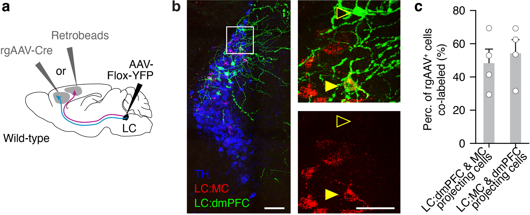
a, Schematic of experimental design for tracing experiments. We injected rgAAV-Cre and retrobeads into dmPFC or MC and quantified co-labeled TH+ neurons in the LC. b, Representative image of TH+ LC neurons (blue) with neurons projecting to dmPFC labeled with YFP and neurons projecting to MC labeled with red retrobeads. Arrows indicate example neurons, one labeled with just YFP (outlined arrow), another with both YFP and retrobeads (filled arrow). Scale bars: 100 μm left panel, 50 μm right panels. c, Quantification of the percent of YFP+ cells co-labeled with retrobeads when rgAAV-Cre was injected in dmPFC and retrobeads were injected in MC (group 1; n = 4 mice) and when rgAAV-Cre was injected in MC and retrobeads were injected in dmPFC (group 2; n = 4 mice). Data are mean ± s.e.m. in c.

Extended Data Fig.8. LC-NE axonal imaging correlates highly with cortical NE release.

a, Raster plots aligned to the timing of lever press during hit or false alarm trials for LC-NE:dmPFC and LC-NE:MC axons. b, Corresponding session average (shaded areas indicate s.e.m.) for the two examples shown in a. c, Population activity of all LC:dmPFC and LC:MC axons for hit, miss, correct rejection, and false alarm trials, aligned to time of tone. d, Example ROI of two axons recorded simultaneously. and the distance between them. Scale bar: 50 μm. e, Raster plots aligned to the timing of press during hit trials for the two axons shown in d. f, Trial by trial correlation versus distance between axons for all simultaneously recorded axons in the LC-NE:MC and LC-NE:dmPFC conditions. P value for Pearson correlation = 0.537. Note the similar trial-by-trial correlation between the two conditions. g, Example ROI of two segments from the same axon from the LC-NE:MC condition. Scale bar: 50 μm. h, Session average during hit (left) or false alarm (right) for the two axonal segments in g, compared with the signal from the entire axon. i, Comparison of the correlation between the signal from an axonal segment and the signal from the entire visible part of the axon. Note the high correlation for both conditions indicating that within-axon Ca²⁺ dynamics are low. j, Strategy and schematic for sparse labeling and imaging of GRAB_NE2m in the cortex. k, GRAB_NE2m ΔF/F signal for a full 450 × 450 μm field of view in the MC. Dashed lines indicate timing of lever press for hit or false alarm trials. l,m, Average GRAB_NE2m signal on hit, miss, correct rejection, and false alarm trials, aligned to time of tone in l and the timing of press in m. Solid lines and shaded areas display mean ± s.e.m. n, Normalized cross-correlation (xcorr) of axonal ΔF/F versus average GRAB_NE2m ΔF/F as a function of lag between the two signals during false alarm (FA) and hit trials. o, Pearson r correlation for axonal ΔF/F versus average GRAB_NE2m ΔF/F during false alarm and hit trials. 33/44 LC:MC axons were significantly correlated with GRAB_NE2m signal (P < 0.05, two-tailed, from Pearson’s correlation). n = 43 LC:MC and 34 LC:dmPFC axons from 4 mice each in c. n = 71 axonal pairs in f. n = 8 LC:MC and 7 LC:dmPFC axons from 4 mice each in i. n = average GRAB_NE2m signal from 4 mice in l,m,n,o. n = 43 LC:MC axons in m,o. Data are mean ± s.e.m. in b, l, m, n. Box plot parameters as in Extended data Fig. 1.

Extended Data Fig. 9. MC is involved in the behavioral response.

a, Muscimol (GABA_A receptor agonist) or saline (control) were locally injected in the MC of both hemispheres. b, 90 to 120 minutes after injection, we tested the mouse performance on the go/no-go auditory detection task. c, Coronal slices at the level of MC showing the extent of our local injection with fluorescein, a fluorophore with a similar molecular weight than muscimol. Scale bars: 1 mm. d, Probability of pressing (P(press)) for different go or no-go tone intensities (s_Go or s_NoGo respectively) for an example mouse. Each dot displays the average, and each solid line displays the results of the logistic regression for P(press) using s_Go or s_NoGo as regressors. e, Change in P(press) following muscimol injections in MC from saline injected controls. Data are mean ± 95% confidence intervals determined by bootstrapping. P values were calculated using two-tailed Wilcoxon signed-rank test (vs. baseline). f, Change in average false alarm, hit rate, and d-prime following muscimol injection in MC. P = 0.031 (false alarm), 0.016 (hit), and 0.016 (d-prime) using one-sided Wilcoxon test of saline versus muscimol condition. g, Coronal sections at the LC, MC – forelimb, and dmPFC levels showing Jaws-tdTomato in LC and fiber location above MC and dmPFC. Scale bars = 1 mm. h, Example axonal expression of Jaws-tdTomato in the dmPFC. Scale bar = 20 μm. i, Effect of LC-NE photoinhibition on the change in d-prime following different trial types. Delta d-prime was calculated by subtracting the average d-prime measured after a certain reinforcement to the global d-prime measured by shuffling trial sequences. n = 6 mice in e,f. n = 7 and 5 mice for LC-NE:dmPFC and MC photoinhibition respectively in i.

Extended Data Fig.10. Summary of spatiotemporal dynamics of LC-NE in learned behavior.

a, In a sensory-motor task, LC-NE neurons are transiently activated during the execution (lever press) and following a positive or negative reinforcement. The execution activity scales up while the reward response scales down with sensory evidence. Negative reinforcement produces the largest LC-NE response during the task regardless of sensory evidence. b, Temporal (top) and spatial (bottom) dynamics of LC-NE during learned behavior. LC-NE signals to cortical outputs are targeted modularly to motor cortex during press and distributed focally or broadly following reward or punishment respectively. These distinct spatiotemporal dynamics facilitate task execution (lever movement) and serial response bias.

Data availability

All data are available from the corresponding authors upon reasonable request. Source data are provided with this paper.

References:

- 1.Poe GR et al. Locus coeruleus: a new look at the blue spot. Nature Reviews Neuroscience 21, 644–659, doi: 10.1038/s41583-020-0360-9 (2020). [DOI] [PMC free article] [PubMed] [Google Scholar]
- 2.Aston-Jones G & Cohen JD An Integrative Theory of Locus Coeruleus-Norepinephrine Function: Adaptive Gain and Optimal Performance. Annual Review of Neuroscience 28, 403–450, doi: 10.1146/annurev.neuro.28.061604.135709 (2005). [DOI] [PubMed] [Google Scholar]
- 3.Sara SJ The locus coeruleus and noradrenergic modulation of cognition. Nature Reviews Neuroscience 10, 211–223, doi: 10.1038/nrn2573 (2009). [DOI] [PubMed] [Google Scholar]
- 4.Breton-Provencher V, Drummond GT & Sur M Locus Coeruleus Norepinephrine in Learned Behavior: Anatomical Modularity and Spatiotemporal Integration in Targets. Frontiers in Neural Circuits 15, doi: 10.3389/fncir.2021.638007 (2021). [DOI] [PMC free article] [PubMed] [Google Scholar]
- 5.Jones BE Arousal and sleep circuits. Neuropsychopharmacology 45, 6–20, doi: 10.1038/s41386-019-0444-2 (2020). [DOI] [PMC free article] [PubMed] [Google Scholar]
- 6.Hayat H et al. Locus coeruleus norepinephrine activity mediates sensory-evoked awakenings from sleep. Science Advances 6, eaaz4232, doi: 10.1126/sciadv.aaz4232 (2020). [DOI] [PMC free article] [PubMed] [Google Scholar]
- 7.Breton-Provencher V & Sur M Active control of arousal by a locus coeruleus GABAergic circuit. Nature Neuroscience 22, 218–228, doi: 10.1038/s41593-018-0305-z (2019). [DOI] [PMC free article] [PubMed] [Google Scholar]
- 8.Reimer J et al. Pupil fluctuations track rapid changes in adrenergic and cholinergic activity in cortex. Nature Communications 7, 13289, doi: 10.1038/ncomms13289 (2016). [DOI] [PMC free article] [PubMed] [Google Scholar]
- 9.Usher M, Cohen JD, Servan-Schreiber D, Rajkowski J & Aston-Jones G The Role of Locus Coeruleus in the Regulation of Cognitive Performance. Science 283, 549, doi: 10.1126/science.283.5401.549 (1999). [DOI] [PubMed] [Google Scholar]
- 10.Bouret S & Sara SJ Reward expectation, orientation of attention and locus coeruleus-medial frontal cortex interplay during learning. European Journal of Neuroscience 20, 791–802, doi: 10.1111/j.1460-9568.2004.03526.x (2004). [DOI] [PubMed] [Google Scholar]
- 11.Rodenkirch C, Liu Y, Schriver BJ & Wang Q Locus coeruleus activation enhances thalamic feature selectivity via norepinephrine regulation of intrathalamic circuit dynamics. Nature Neuroscience 22, 120–133, doi: 10.1038/s41593-018-0283-1 (2019). [DOI] [PMC free article] [PubMed] [Google Scholar]
- 12.Uematsu A et al. Modular organization of the brainstem noradrenaline system coordinates opposing learning states. Nature Neuroscience 20, 1602–1611, doi: 10.1038/nn.4642 (2017). [DOI] [PubMed] [Google Scholar]
- 13.Likhtik E & Johansen JP Neuromodulation in circuits of aversive emotional learning. Nature Neuroscience 22, 1586–1597, doi: 10.1038/s41593-019-0503-3 (2019). [DOI] [PubMed] [Google Scholar]
- 14.Kaufman AM, Geiller T & Losonczy A A Role for the Locus Coeruleus in Hippocampal CA1 Place Cell Reorganization during Spatial Reward Learning. Neuron 105, 1018–1026.e1014, doi: 10.1016/j.neuron.2019.12.029 (2020). [DOI] [PMC free article] [PubMed] [Google Scholar]
- 15.Takeuchi T et al. Locus coeruleus and dopaminergic consolidation of everyday memory. Nature 537, 357–362, doi: 10.1038/nature19325 (2016). [DOI] [PMC free article] [PubMed] [Google Scholar]
- 16.Wagatsuma A et al. Locus coeruleus input to hippocampal CA3 drives single-trial learning of a novel context. Proceedings of the National Academy of Sciences 115, E310, doi: 10.1073/pnas.1714082115 (2018). [DOI] [PMC free article] [PubMed] [Google Scholar]
- 17.McCall, Jordan G. et al. CRH Engagement of the Locus Coeruleus Noradrenergic System Mediates Stress-Induced Anxiety. Neuron 87, 605–620, doi: 10.1016/j.neuron.2015.07.002 (2015). [DOI] [PMC free article] [PubMed] [Google Scholar]
- 18.Bouret S & Sara SJ Network reset: a simplified overarching theory of locus coeruleus noradrenaline function. Trends in Neurosciences 28, 574–582, doi: 10.1016/j.tins.2005.09.002 (2005). [DOI] [PubMed] [Google Scholar]
- 19.Yu AJ & Dayan P Uncertainty, Neuromodulation, and Attention. Neuron 46, 681–692, doi: 10.1016/j.neuron.2005.04.026 (2005). [DOI] [PubMed] [Google Scholar]
- 20.Dayan P & Yu AJ Phasic norepinephrine: A neural interrupt signal for unexpected events. Network: Computation in Neural Systems 17, 335–350, doi: 10.1080/09548980601004024 (2006). [DOI] [PubMed] [Google Scholar]
- 21.Clayton EC, Rajkowski J, Cohen JD & Aston-Jones G Phasic Activation of Monkey Locus Ceruleus Neurons by Simple Decisions in a Forced-Choice Task. The Journal of Neuroscience 24, 9914, doi: 10.1523/JNEUROSCI.2446-04.2004 (2004). [DOI] [PMC free article] [PubMed] [Google Scholar]
- 22.Kalwani RM, Joshi S & Gold JI Phasic Activation of Individual Neurons in the Locus Ceruleus/Subceruleus Complex of Monkeys Reflects Rewarded Decisions to Go But Not Stop. The Journal of Neuroscience 34, 13656, doi: 10.1523/JNEUROSCI.2566-14.2014 (2014). [DOI] [PMC free article] [PubMed] [Google Scholar]
- 23.Bornert P & Bouret S Locus coeruleus neurons encode the subjective difficulty of triggering and executing actions. PLOS Biology 19, e3001487, doi: 10.1371/journal.pbio.3001487 (2021). [DOI] [PMC free article] [PubMed] [Google Scholar]
- 24.McGinley Matthew J., David Stephen V. & McCormick David A. Cortical Membrane Potential Signature of Optimal States for Sensory Signal Detection. Neuron 87, 179–192, doi: 10.1016/j.neuron.2015.05.038 (2015). [DOI] [PMC free article] [PubMed] [Google Scholar]
- 25.Martins ARO & Froemke RC Coordinated forms of noradrenergic plasticity in the locus coeruleus and primary auditory cortex. Nature Neuroscience 18, 1483–1492, doi: 10.1038/nn.4090 (2015). [DOI] [PMC free article] [PubMed] [Google Scholar]
- 26.Bari A et al. Differential attentional control mechanisms by two distinct noradrenergic coeruleo-frontal cortical pathways. Proceedings of the National Academy of Sciences 117, 29080–29089, doi: 10.1073/pnas.2015635117 (2020). [DOI] [PMC free article] [PubMed] [Google Scholar]
- 27.Vazey EM, Moorman DE & Aston-Jones G Phasic locus coeruleus activity regulates cortical encoding of salience information. Proceedings of the National Academy of Sciences 115, E9439, doi: 10.1073/pnas.1803716115 (2018). [DOI] [PMC free article] [PubMed] [Google Scholar]
- 28.Aston-Jones G & Bloom FE Norepinephrine-containing locus coeruleus neurons in behaving rats exhibit pronounced responses to non-noxious environmental stimuli. The Journal of Neuroscience 1, 887, doi: 10.1523/JNEUROSCI.01-08-00887.1981 (1981). [DOI] [PMC free article] [PubMed] [Google Scholar]
- 29.Tervo Dougal G. R. et al. Behavioral Variability through Stochastic Choice and Its Gating by Anterior Cingulate Cortex. Cell 159, 21–32, doi: 10.1016/j.cell.2014.08.037 (2014). [DOI] [PubMed] [Google Scholar]
- 30.Urai AE, Braun A & Donner TH Pupil-linked arousal is driven by decision uncertainty and alters serial choice bias. Nature Communications 8, 14637, doi: 10.1038/ncomms14637 (2017). [DOI] [PMC free article] [PubMed] [Google Scholar]
- 31.Krishnamurthy K, Nassar MR, Sarode S & Gold JI Arousal-related adjustments of perceptual biases optimize perception in dynamic environments. Nature Human Behaviour 1, 0107, doi: 10.1038/s41562-017-0107 (2017). [DOI] [PMC free article] [PubMed] [Google Scholar]
- 32.Schwarz LA et al. Viral-genetic tracing of the input–output organization of a central noradrenaline circuit. Nature 524, 88–92, doi: 10.1038/nature14600 (2015). [DOI] [PMC free article] [PubMed] [Google Scholar]
- 33.Plummer NW et al. An Intersectional Viral-Genetic Method for Fluorescent Tracing of Axon Collaterals Reveals Details of Noradrenergic Locus Coeruleus Structure. eneuro 7, ENEURO.0010-0020.2020, doi: 10.1523/ENEURO.0010-20.2020 (2020). [DOI] [PMC free article] [PubMed] [Google Scholar]
- 34.Kebschull JM et al. High-Throughput Mapping of Single-Neuron Projections by Sequencing of Barcoded RNA. Neuron 91, 975–987, doi: 10.1016/j.neuron.2016.07.036 (2016). [DOI] [PMC free article] [PubMed] [Google Scholar]
- 35.Chandler DJ, Gao W-J & Waterhouse BD Heterogeneous organization of the locus coeruleus projections to prefrontal and motor cortices. Proceedings of the National Academy of Sciences 111, 6816, doi: 10.1073/pnas.1320827111 (2014). [DOI] [PMC free article] [PubMed] [Google Scholar]
- 36.Spencer RC, Devilbiss DM & Berridge CW The Cognition-Enhancing Effects of Psychostimulants Involve Direct Action in the Prefrontal Cortex. Biological Psychiatry 77, 940–950, doi: 10.1016/j.biopsych.2014.09.013 (2015). [DOI] [PMC free article] [PubMed] [Google Scholar]
- 37.Totah NK, Neves RM, Panzeri S, Logothetis NK & Eschenko O The Locus Coeruleus Is a Complex and Differentiated Neuromodulatory System. Neuron 99, 1055–1068.e1056, doi: 10.1016/j.neuron.2018.07.037 (2018). [DOI] [PubMed] [Google Scholar]
- 38.Kamigaki T & Dan Y Delay activity of specific prefrontal interneuron subtypes modulates memory-guided behavior. Nature Neuroscience 20, 854–863, doi: 10.1038/nn.4554 (2017). [DOI] [PMC free article] [PubMed] [Google Scholar]
- 39.Huber D et al. Multiple dynamic representations in the motor cortex during sensorimotor learning. Nature 484, 473–478, doi: 10.1038/nature11039 (2012). [DOI] [PMC free article] [PubMed] [Google Scholar]
- 40.Goard MJ, Pho GN, Woodson J & Sur M Distinct roles of visual, parietal, and frontal motor cortices in memory-guided sensorimotor decisions. eLife 5, e13764, doi: 10.7554/eLife.13764 (2016). [DOI] [PMC free article] [PubMed] [Google Scholar]
- 41.Akrami A, Kopec CD, Diamond ME & Brody CD Posterior parietal cortex represents sensory history and mediates its effects on behaviour. Nature 554, 368–372, doi: 10.1038/nature25510 (2018). [DOI] [PubMed] [Google Scholar]
- 42.Hattori R, Danskin B, Babic Z, Mlynaryk N & Komiyama T Area-Specificity and Plasticity of History-Dependent Value Coding During Learning. Cell 177, 1858–1872.e1815, doi: 10.1016/j.cell.2019.04.027 (2019). [DOI] [PMC free article] [PubMed] [Google Scholar]
- 43.Bari BA et al. Stable Representations of Decision Variables for Flexible Behavior. Neuron 103, 922–933.e927, doi: 10.1016/j.neuron.2019.06.001 (2019). [DOI] [PMC free article] [PubMed] [Google Scholar]
- 44.Park AJ et al. Reset of hippocampal–prefrontal circuitry facilitates learning. Nature 591, 615–619, doi: 10.1038/s41586-021-03272-1 (2021). [DOI] [PMC free article] [PubMed] [Google Scholar]
- 45.Waterhouse BD, Moises HC & Woodward DJ Phasic activation of the locus coeruleus enhances responses of primary sensory cortical neurons to peripheral receptive field stimulation. Brain Research 790, 33–44, doi:https://doi.org/10.1016/S0006-8993(98)00117-6 (1998). [DOI] [PubMed] [Google Scholar]
- 46.Hangya B, Ranade Sachin P., Lorenc M & Kepecs A Central Cholinergic Neurons Are Rapidly Recruited by Reinforcement Feedback. Cell 162, 1155–1168, doi: 10.1016/j.cell.2015.07.057 (2015). [DOI] [PMC free article] [PubMed] [Google Scholar]
- 47.Matias S, Lottem E, Dugué GP & Mainen ZF Activity patterns of serotonin neurons underlying cognitive flexibility. eLife 6, e20552, doi: 10.7554/eLife.20552 (2017). [DOI] [PMC free article] [PubMed] [Google Scholar]
- 48.Schultz W, Dayan P & Montague PR A Neural Substrate of Prediction and Reward. Science 275, 1593, doi: 10.1126/science.275.5306.1593 (1997). [DOI] [PubMed] [Google Scholar]
- 49.Cohen JY, Haesler S, Vong L, Lowell BB & Uchida N Neuron-type-specific signals for reward and punishment in the ventral tegmental area. Nature 482, 85–88, doi: 10.1038/nature10754 (2012). [DOI] [PMC free article] [PubMed] [Google Scholar]
- 50.Keiflin, R. & Janak, Patricia H. Dopamine Prediction Errors in Reward Learning and Addiction: From Theory to Neural Circuitry. Neuron 88, 247–263, doi: 10.1016/j.neuron.2015.08.037 (2015). [DOI] [PMC free article] [PubMed] [Google Scholar]
- 51.Tai L-H, Lee AM, Benavidez N, Bonci A & Wilbrecht L Transient stimulation of distinct subpopulations of striatal neurons mimics changes in action value. Nature Neuroscience 15, 1281–1289, doi: 10.1038/nn.3188 (2012). [DOI] [PMC free article] [PubMed] [Google Scholar]
- 52.Barbosa J et al. Interplay between persistent activity and activity-silent dynamics in the prefrontal cortex underlies serial biases in working memory. Nature Neuroscience 23, 1016–1024, doi: 10.1038/s41593-020-0644-4 (2020). [DOI] [PMC free article] [PubMed] [Google Scholar]
Methods references
- 53.Dana H et al. High-performance calcium sensors for imaging activity in neuronal populations and microcompartments. Nature Methods 16, 649–657, doi: 10.1038/s41592-019-0435-6 (2019). [DOI] [PubMed] [Google Scholar]
- 54.Feng J et al. A Genetically Encoded Fluorescent Sensor for Rapid and Specific In Vivo Detection of Norepinephrine. Neuron 102, 745–761.e748, doi: 10.1016/j.neuron.2019.02.037 (2019). [DOI] [PMC free article] [PubMed] [Google Scholar]
- 55.Carlén M What constitutes the prefrontal cortex? Science 358, 478, doi: 10.1126/science.aan8868 (2017). [DOI] [PubMed] [Google Scholar]
- 56.Barthas F & Kwan AC Secondary Motor Cortex: Where ‘Sensory’ Meets ‘Motor’ in the Rodent Frontal Cortex. Trends in Neurosciences 40, 181–193, doi: 10.1016/j.tins.2016.11.006 (2017). [DOI] [PMC free article] [PubMed] [Google Scholar]
- 57.Slotnick B A SIMPLE 2-TRANSISTOR TOUCH OR LICK DETECTOR CIRCUIT. Journal of the Experimental Analysis of Behavior 91, 253–255, doi: 10.1901/jeab.2009.91-253 (2009). [DOI] [PMC free article] [PubMed] [Google Scholar]
- 58.El-Boustani S et al. Locally coordinated synaptic plasticity of visual cortex neurons in vivo. Science 360, 1349, doi: 10.1126/science.aao0862 (2018). [DOI] [PMC free article] [PubMed] [Google Scholar]
- 59.Lovett-Barron M et al. Ancestral Circuits for the Coordinated Modulation of Brain State. Cell 171, 1411–1423.e1417, doi: 10.1016/j.cell.2017.10.021 (2017). [DOI] [PMC free article] [PubMed] [Google Scholar]
- 60.Kvitsiani D et al. Distinct behavioural and network correlates of two interneuron types in prefrontal cortex. Nature 498, 363–366, doi: 10.1038/nature12176 (2013). [DOI] [PMC free article] [PubMed] [Google Scholar]
- 61.Chung JE et al. A Fully Automated Approach to Spike Sorting. Neuron 95, 1381–1394.e1386, doi: 10.1016/j.neuron.2017.08.030 (2017). [DOI] [PMC free article] [PubMed] [Google Scholar]
- 62.Schneider CA, Rasband WS & Eliceiri KW NIH Image to ImageJ: 25 years of image analysis. Nature Methods 9, 671–675, doi: 10.1038/nmeth.2089 (2012). [DOI] [PMC free article] [PubMed] [Google Scholar]
- 63.Marks TD & Goard MJ Stimulus-dependent representational drift in primary visual cortex. Nature Communications 12, 5169, doi: 10.1038/s41467-021-25436-3 (2021). [DOI] [PMC free article] [PubMed] [Google Scholar]
- 64.Engelhard B et al. Specialized coding of sensory, motor and cognitive variables in VTA dopamine neurons. Nature 570, 509–513, doi: 10.1038/s41586-019-1261-9 (2019). [DOI] [PMC free article] [PubMed] [Google Scholar]
- 65.Musall S, Kaufman MT, Juavinett AL, Gluf S & Churchland AK Single-trial neural dynamics are dominated by richly varied movements. Nature Neuroscience 22, 1677–1686, doi: 10.1038/s41593-019-0502-4 (2019). [DOI] [PMC free article] [PubMed] [Google Scholar]
- 66.Pho GN, Goard MJ, Woodson J, Crawford B & Sur M Task-dependent representations of stimulus and choice in mouse parietal cortex. Nature Communications 9, 2596, doi: 10.1038/s41467-018-05012-y (2018). [DOI] [PMC free article] [PubMed] [Google Scholar]
Associated Data
This section collects any data citations, data availability statements, or supplementary materials included in this article.
Data Availability Statement