

Abstract
This paper introduces a new method to describe and analyse multidimensional time series based on wavelets. The methodology considers the time series as observations of a functional random variable. The paper generalizes previous research on stock market networks by including asset returns and volume trading as the main variables to study the financial market. The methodology is applied to examine the dynamics and structure of the Nasdaq-100 stock market during the pandemic period 2019/12–2021/12 considering both asset returns and volume trading to model the behaviour of different assets that are part of the index, applying an algorithm that offers better performance than others applied in the clustering literature. The study detects four clusters of firms corresponding with companies sharing common economic activities. The structure of the network reveals a nonlinear relationship between the variables, and the study shows that the main macroeconomic events during the period affect each cluster with different intensity. The change in the patterns of returns and risks and the redistribution of wealth in a highly changing environment are emerging phenomena, which must necessarily be carefully analyzed by public policies, in order to avoid the appearance of bubbles and systemic shocks.
Keywords: Clustering finance, Multivariate times series, Nasdaq-100 stock market, Portfolios construction, Wavelets
Introduction
Most financial models focus on asset returns or prices, without paying attention to the volume traded. However, considering the volumes traded may offer information not contained in prices. As indicated by Karpoff (1987), relating the prices with the volumes traded allows knowing the flow of information and the efficiency in the asset markets. The relationship between prices and volumes in different time frames is extremely significant because the joint dynamics of both variables can provide additional information than would be obtained by analyzing them separately.
Far from this interest in analyzing the behaviour of the volume traded, developments arise from the efficient market hypothesis. It was firstly developed by Fama (1970) and establishes that under an informational efficient market, the price of financial assets reflects all the relevant information known by the members of the market and also reflects all beliefs about the future. As a consequence, the flow of information that will determine the price of the shares behaves like a random walk, as in Fama (1965). Irrational behaviors and large deviations are compatible with this hypothesis, provided that these biases and deviations are not predictable.
In this paper, a new clustering methodology is presented for process data, particularly multivariate time series data. The methodology is applied to examine the behaviour of joint movements in prices and volumes for Nasdaq-100 stock exchange between December 2019 and December 2021. A stock exchange is a location where company shares are traded; it provides a platform, which can be a corporation or a mutual organization, where members of the organization trade stocks and other securities. The majority of the world’s leading economic nations have their own stock markets. Nasdaq-100 and the New York Stock Exchange (NYSE) are the two largest stock exchanges in the world. On the other hand, as Bui and Ślepaczuk (2022), Nasdaq-100 index was that it was one of the most volatile, diversified and well performing index during the last 30 years. Also, as in Gómez-Martínez et al. (2022), The Nasdaq-100 index was chosen as the subject of study because technology companies represent a significant component of the index and have become a substantial economic influence. In addition, it offers a database of excellent quality that has been utilized in a variety of analyses, as we review in the next section.
It is assumed that the database contains sets of time-series data, which correspond to different periods of process operation, for example different batches produced by a batch process. The clustering methodology is based on calculating the degree of similarity using principal component analysis (PCA) and distance similarity factors. The proposed methodology identifies different groups according to the type of companies and capitalization. The empirical results suggest that some groups of assets are more sensitive to fluctuations in prices and quantities traded during periods of crisis, and that a non-linear relationship in the variation of prices and volumes must be considered.
The paper is organized as follows. We first review the literature on the link between volumes and prices in exchange markets and a brief review about clustering methods in Sect. 2. In Sect. 3 mathematical concepts are introduced and our approach is presented in Sect. 4. Section 5 describe two simulation examples and in Sect. 6, results are shown using the new methodology and data from Nasdaq-100. In Sect. 7 we present the final conclusions.
Summary of literature review
This section reviews two topics on which this article is based: the relationship between price and volume in financial series and a brief review of clustering techniques. The wavelet techniques utilized in this article are discussed in greater detail in Sect. 3.
Empirical evidence regarding the price-volume interaction
This section’s literature review is an expansion of Karpoff (1987) article, as it shows the implementation of novel methodologies since the 1990s. This article also illustrates an application of the wavelet technique to the case of the price-quantity link.
Since the 1960s, the relationship between prices and volumes has been studied. First results (Godfrey et al. 1964; Granger and Morgenstern 1963; Ying 1966) do not find a correlation between prices and volumes. Then, studies suggest that a correlation exists between volume and the absolute value of the price change, . This phenomenon is related to the famous phrase “it takes volume to make prices move” (Clark 1973; Crouch 1970). Later studies (Epps 1975, 1977) show that the relationship is with , without taking into account the absolute value. It is even found that volume is higher when prices increase than when prices decrease (Epps 1975; Harris 1987; Jain and Joh 1988). There are theoretical developments that seek to explain these movements, such as Copeland’s (1976) model of sequential arrival of information. In Jennings and Barry (1983), the author proposes an extension to this model, that allows the possibility of speculative (short) positions. Other developments, such as Clark (1973); Epps and Epps (1976) analyze the possibility that the results obtained in the distribution of price variations of speculative assets are the consequence of the union of a set of distributions with different variances, which forms the “mixture of distributions hypothesis”. Other authors, such as Lam and Ang (1995), explains this relationship due to short-selling practices. Finally, authors such as Pfleiderer (1984) show the importance of multiple life-cycle trading and the results are consistent with a rational expectations equilibrium with life cycle trading.
Starting in the 1990s, the causal relationship between returns and volume began to be analyzed. Is important to know whether or not there exists a directional information transfer between stock prices and trading volume. In the case of existence, knowledge of past movements in stock prices could lead to improved predictions not only of current but also future movements in trading volume, and vice versa. Most of the papers developed from these ideas are based on empirical work, where Vector Autorregressions and Granger causality tests are applied. The results are not conclusive, because authors such as Chuang et al. (2009), Smirlock and Starks (1988), Statman et al. (2006) find causality from absolute price changes to volume, while (Hutson et al. 2008; Saatcioglu and Starks 1998) find causality from volume to returns. In this sense, a critique of previous studies is applied by Behrendt and Schmidt (2021), since it proposes that VAR and Granger causality tests do not take into account the non-linear nature of this relation. It can be assumed, as in Brida et al. (2016); Brida and Risso (2009) that this relationship may be different between different groups of assets. There is evidence that many of these relationships between assets are maintained in periods of great financial stress, as in Lahmiri (2012), Zhao et al. (2016). Similarly, it is found in Lahmiri (2012) that there is an evolution in the links between financial assets. The literature on this topic focuses only on the relationships between asset returns (among other examples, see (Dias et al. 2015; Tabak et al. 2010)) and finds that asset groups are related to the industrial activity performed.
Clustering in time-series
The clustering methods are more difficult than supervised learning methods since there is no label attached to the patterns in the clustering. Moreover, in Kleinberg (2002), three axioms are proposed that a clustering procedure should verify and it is proved that no method simultaneously fulfills all three. This shows that in general there is no optimal clustering method and each particular clustering algorithm is targeted at a particular set of applications.
Two categories of clustering can be distinguished: hard clustering (each observation is in a single group ) and soft clustering (each observation can be contained in more than one cluster). There are many clustering algorithms in the literature which can be broadly classified as follows, Partitional Clustering, Hierarchical Clustering, Density-Based Clustering, Grid-Based Clustering and Model-Based Clustering, see (Ghosal et al. 2020).
There are a large number of recent applications in different areas of science such as medicine and finance, see for instance (Abdullah et al. 2022; Mansano et al. 2022) respectively. Clustering methods have also been designed for high dimensional data [see (Mittal et al. 2019)] or infinite dimensional data, see for instance (Jacques and Preda 2014; Fortuna and Maturo 2019). A review of different clustering methodologies is given for example (Saxena et al. 2017; Mehta et al. 2020).
In particular the analysis on time-series clustering methods has increased considerably over the last two decades with a wide range of applications in many different fields, including geology, environmental sciences, finance, economics, and biomedical sciences. Clustering of time series can technically be put into three groups, viz., methods based on the actual observations, on features derived for the time series and on parameters estimates of fitted models. In this context, several statistical methodologies have been used to generate clustering on these time series, see as a general reference (Maharaj et al. 2019). The usefulness of these techniques has stimulated the generation of different works both in the field of univariate series [see, for instance, Aghabozorgi et al. (2015; Alonso and Peña 2019; Iglesias and Kastner 2013)] and their computational implementations [see (Montero and Vilar 2015; Sardá-Espinosa 2017)].
There are also some generalizations for multivariate series [see (D’Urso and Pierpaolo Massari 2018; Li 2019; Singhal and Seborg 2005)]. In particular, a method with good performance is the projection of the univariate series (in a finite dimensional space) by its expansion (truncated) through Wavelets, see (Ann Maharaj et al. 2010; Hong-fa 2012; Zhang et al. 2006). The reason for this is that the modeling of univariate financial series by means of wavelets is of great relevance even in recent research, see (Kuşkaya et al. 2022). In this direction, there are also different alternatives to generate multivariate series clusters, see (Barragan et al. 2016; D’Urso and Maharaj 2012). We propose a variant of these techniques, based on a generalization of Berlinet et al. (2008) for multivariate functionals and in a clustering context.
Preliminary concepts
This section introduces the mathematical notation and the main definitions used in the study. The first step is to represent the multivariate financial series as functional data, by using the functional data analysis (FDA). These data are characterized as a high dimensional vector with a high correspondence between its components. The second step is select a technique for reduction of dimensionality of the data. For reasons of treatability, we need to immerse the data in a finite dimensional space, with the minimum loss of information. To this aim, a truncation of the development using wavelets is performed. This methodology have grown in recent years. The third step is to apply clustering techniques to separate the multivariate data dynamics into groups according to their similarity. These techniques are applied in these finite-dimensional spaces and the results are extrapolated to the infinite dimensional space.
In the last two decades the development of statistics in functional spaces has grown. The opportunity of massive data extraction in short periods of time has made this type of data very frequent. In the financial industry, there is a large amount of historical data on prices, volumes, yields and volatilities is extensive in the various financial markets.
This is a great advantage of this economic area that allows the development of mathematical and statistical solutions to issues related to asset management. A random element is called functional variable if it takes values in an infinite dimensional space . In this work, we consider as a separable Hilbert space (complete space in which an inner product is defined). In particular, we use the Hilbert space
| 1 |
with I a compact interval and
Our objective is to apply classification techniques to multivariate data. However, the classical multivariate classification methods, developed in the 20th century, are not applicable in this context. Two main approaches have been developed to avoid this difficulty. The first approach is to use functional analysis to develop a new theory compatible with this type of data. The second approach involves an appropriate transformation of the data to transform it into a finite-dimensional space and apply the usual techniques. In this paper, the second approach is used to truncate the wavelet development of the financial series, see (Morettin et al. 2017).
When a data X is decomposed into wavelet series, the wavelet coefficients describe the dynamics of a time series in both the time and frequency domains. Unlike the Fourier transform which decomposes the data into a sum of sine and cosine functions that are not resolved in time, wavelet analysis uses a set of functions locally defined in both time and frequency domains. A wavelet basis consists of a mother function which is dilated and shifted to build different levels of resolution. The idea was to construct local basis functions that could be shifted and scaled and then reassembled to approximate a given signal. Most applications in finance are related to econometrics; however, there is a strong development in asset pricing that is important for academic researchers and finance practitioners. Using the same notation as in Berlinet et al. (2008), we briefly recall wavelet bases for (one dimensional curves). Wavelets are important tool for approximate functions with a basis whose elements are obtained trough translation and dilation operations of a function ,
| 2 |
In Eq. 2, the integer j in the scale indicates the width of the wavelet and the value k gives the location in time. One of the advantages of this type of bases is that, knowing the behavior of the function , it is possible to know the behavior of the entire base.
In particular, given a function , , it is can be expressed by
| 3 |
where and , being the inner product in the space . It is relevant to reindex the numerable base components into Therefore, any random observation is expressed as a series expansion and it is possible rewritten as
| 4 |
with the coefficients
| 5 |
Briefly, it is possible to define the cluster methodology as the search for k groups in n observations based on a measure of similarity. The idea is that the similarity between objects of the same group is large while the similarity between objects of different groups is small. The aim of cluster analysis is to find “similar” groups of observations. In this work, we use the unsupervised clustering (concept introduced by Tyron in 1939). Several methodologies have been proposed to analyze the problem of clustering in functional data, see (Jacques and Preda 2014). For it, we define the similarity between two functional observations through the closeness of the coefficients (of larger magnitudes) of the truncated wavelet expansion of both series (price and volume).
Methodology
As stated in the introduction, our objective is to group the joint price and volume dynamics of several Nasdaq-100 companies. The main methodological contribution in this work is the extension of the proposed method in Berlinet et al. (2008) to the case of multivariate series and in the unsupervised clustering context. This methodology for cluster is based on a reduction of the dimensionality from the use of wavelets and the determination of the clusters is carried out using the partition around medoids (PAM) method .
We need to analyze the case of two dimensions, i.e. , following the methodology proposed by Berlinet et al. (2008) for one dimension. Let consider the base therefore,
| 6 |
In our quest of dimension reduction, we fix the resolution level J in both marginal distributions the truncated series is
| 7 |
It important reorder the first basis functions via the scheme,
| 8 |
with . This ordering allows establishing which basic functions carry the most significant information. Lastly, it is selected the effective dimension , and approximating each by . In this way we obtain a finite dimensional approximation in dimension d of the multivariate series to later be able to use the classic clustering procedures. We select the Partition Around Medoid (PAM) method, which has arguments similar to , minimizing the differences within each group. The method is intended to find a sequence of objects called medoids that are centrally located in clusters. In particular, the center is a data of the sample, which will allow us a better interpretability of each cluster analyzing its center, see (Kaufman and Rousseeuw 1990).
On the other hand, a challenging problem in clustering is determining the optimal number of the groups. The most used methods are Elbow method, Average silhouette method, Gap statistic method and prediction strength. Different criteria for its validation statistics have been proposed, based on internal validation measures (reflect often the compactness and the separation of the cluster partitions) and on external measures (compare the assigned group with an external reference); see for example (Charrad et al. 2014; Kaufman and Rousseeuw 1990). In our context the problem is even more complex, since it is necessary to adequately estimate the truncation parameter d. In this work we propose an external validation criterion based on the Rand Index (Rand 1971). This index computes a similarity measure between two clusterings by considering all pairs of samples and counting pairs that are assigned in the same or different clusters in the predicted and true clusterings. Briefly, this is a graphic method [for more details see (Zappia and Oshlack 2018)] where the stability of the clusters is observed when the parameter d (dimension) and k (number of cluster) change.
If we consider P and Q two partitions of a set S, the number of pairs of elements in S that are in the same cluster in P and in the same cluster in Q, and the number of pairs of elements in S that are in different clusters in P and in different clusters in Q. The Rand index is
where n is the number of observations. The d and k that maximize the index is selected according to Zappia and Oshlack (2018) and following the parsimony criterion.
Simulation data
In order to evaluate different clustering techniques, a case study was performed based on a simulated bidimensional functional data (price and volume) where the grid simulation has 513 discrete points (two years of daily data). We consider two clusters with forty curves each . The functions are defined such as the process
| 9 |
where k is the cluster and j is the coordinate. Besides, we assume that
| 10 |
and the process are independent identically distributed and satisfies that
| 11 |
where , and the functions are
Finally, we assume that the correlation between the components in time is for all .
The simulated marginal data separated into their respective clusters are shown in Fig. 1. Following the methodology proposed, a joint development is performed using Wavelets and the optimal truncation value estimated by Rand Index is . Finally, two clusters are determined using PAM technique and the original groups are compared with those obtained through the percentage of error in the predictions.
Fig. 1.

Marginal trajectories of the observations of each cluster with respect to a Price b Volume
In Fig. 2, we observe the marginal trajectories of the medoids of each cluster. It is important to note that although the processes are different, the trajectories (mainly in the volume coordinate) show similarities between the clusters. This property is important at the moment of analyzing the performance of the methodology. A perspective variant, in Fig. 3 we observe the curves in two dimensions by varying the time after smoothing the series by cubic splines.
Fig. 2.

Marginal medoids (obtained by PAM) plot Price-Volume. a Cluster 1. b Cluster 2
Fig. 3.

Joint medoids curves (obtained by PAM) Price-Volume. a Cluster 1. b Cluster 2
With the aim to measure the performance of the proposed algorithm, the classification error of our algorithm (called multivariate wavelets clustering) is compared with three classical methods in clusters in functional data. Some key definitions are introduced here in order to evaluate the performance of the methodologies considered in this work. The first method is the naïve approach to the problem and it is called functPAM-cluster. In this method the challenge is to determine a matrix of distances between the data and then use the PAM algorithm. The distance used is that induced by the inner product in the product space .
The second method, which we call EM-cluster, consists in shifting the functions of into the space by considering the function on as follows
| 12 |
This modification allows us to apply the clustering method to functionals with real paths. In this case, the functional principal component (FPC) scores obtained from the data FPC analysis are used, see (Chen et al. 2015). The method developed in this work is called MW-cluster. The fourth method is the use of the so-called symbolic clusters that we will call Symbolic-cluster, see (Brida et al. 2020). In this case the path of the functional is divided into quadrants and each curve is represented with a sequence of numbers according to the quadrant it crosses as a function of time. Subsequently, a hierarchical clustering algorithm is implemented from a defined distance between these sequences, see (Brida et al. 2009; Gowda and Diday 1991).
Through 1000 simulations, the proportion of error committed by each method in each one of the simulations is determined. The results are shown in Fig. 4. The good performance of the method developed in this work is observed there.
Fig. 4.

Classification errors in the simulated data
Real Data
The descriptive data set
The pandemic has caused a financial shock to the economy. After a phase of uncertainty, where the price and volume had had a high volatility, the returns of the different companies have followed different behaviours. The objective of the work is to determine different patterns of behaviour in the pandemic period with respect to price and volume of Nasdaq-100 daily stock prices (at closing) and trading volume of the stocks.
The database include 88 of the largest domestic and international non-financial companies listed on the Nasdaq-100 Stock Market. For example, the main companies in different business areas are Apple, Amazon, American Airlines, Facebook, Microsoft, Zoom, Moderna, Netflix, Pepsi, Marvell, Tesla and Starbucks. The data are available from within R, using the quantmod R package, see (Ryan et al. 2015). It is relevant to normalize the data in order to be able to compare them and obtain the clusters according to the movements in trend and not by magnitudes. That is
| 13 |
This normalization is frequent in the preprocessing of the information (before clustering), as a way of assigning to equalize the variables that determine the groups.
A simple visualization of the data shows that the behaviour of the companies is far from similar. In particular there are phases very marked by the start of the pandemic, where companies behaved dynamically differently in reference to this shock. For example, we selected three companies which suffered the consequences of the pandemic in different ways: American Airlines (AAL), Netflix (NFLX) and Amazon (AMZN). In Fig. 5, we observe the price and volume from February 2017 to December 2021 for these companies. In the three cases, we found differences in the dynamic trajectories and volatility, essentially in the effects generated by the pandemic. As can be seen in the volume of business transactions, there is greater variability with respect to price. Furthermore, we find that the three companies have a different level of volatility in transactions; this volatility is not constant, but in the case of AAL it changes its structure after the pandemic. The analysis of the prices is similar. Here it is found that, depending on the type of specific activity, it is the dynamics of the company’s market value. The pandemic had, among other consequences, a change in the patterns of consumption of goods and services. One of the most affected items is air transport, due to changes in travel patterns introduced by mobility restrictions.
Fig. 5.

Plot the marginal series: daily stock prices and trading volume of the stocks. a AAL b NFLX c AMZN. Red vertical line indicates the beginning of the pandemic in December 2019
In Fig. 6, we show the dynamic obtained in the three selected companies for both price and volume. We can observe the trend of the series in the 2020-2022 through smoothing by means of cubic splines. If we analyze only this trend behaviour by means of smoothing it can be seen that there is no clear pattern in the trend of the analyzed series. Although it can be seen that a greater number of transactions were carried out in the first months of 2020. This can be explained by the volatility of the financial markets as well as new technologies that emerged in this period.
Fig. 6.

Plot the smooth marginal series (by splines): daily stock prices and trading volume of the stocks. a AAL b NFLX c AMZN . The red vertical line indicates the start of the pandemic in December 2019
Following this description of the trend for the three companies, it is possible to make an interpretable graph of the series as a parametric function of time, see Fig. 7. Subsequently, thus be able to jointly analyze the associated behaviour in both variables (price-volume). As can be seen here, the relationship between prices and quantities traded is far from being linear, while there are moments where a positive relationship (from December 2019 to April 2020), see Fig. 7b, while others with a negative relationship in the evolution of prices and quantities (from December 2019 to August 2020), see Fig. 7a. It is even possible to observe changes in the volumes traded without significant changes in prices (from October 2020 to January 2021), see Fig. 7c.
Fig. 7.

Joint curve Price-Volume a AAL b NFLX c AMZN
Results
This previous description motivates the idea of being able to find and analyze groups of companies with similar dynamics in the pandemic period. For this, using the proposed clustering methodology, we need to select the truncation parameter and the number of clusters. Fig. 8 shows how the Rand index changes by varying the truncation parameters d and the cluster number k. A stabilization is observed at a high value of the index from and . Also, fixed d in 35, the stability of the groups can be visualized in a tree diagram, see (Zappia and Oshlack 2018). Figure 9 , using a cluster tree diagram, provides a visualisation for interrogating the clusters as the resolution increases, see (Zappia and Oshlack 2018). This reinforces the choice of as a plausible estimate for the number of groups.
Fig. 8.

Rand index curves by varying the truncation parameter d for different number of clusters
Fig. 9.
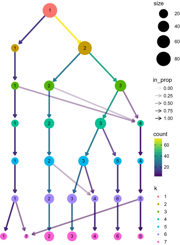
Tree representation of the stability of the groups when increasing the number of groups
The results obtained indicate four clusters where each group has 10, 29, 40 and 6 companies and the centers are FISV, CDNS, TXN and AMGN respectively. Information on these companies can be described as follows: FISV corresponds to the company Fiserv1, with activities in the processing of payments and electronic transfers; CDNS2 is a software company, specialized in the automation of chip design; TXN3 is a company dedicated to the production of semi-conductors while AMGN4 is a company specialized in biotechnology.
As can be seen, the four companies are related to different products and processes within the Nasdaq-100, so the clustering analysis helps to analyze the different dynamics within each sector. At the same time, differences between clusters allow us to analyze how variations in patterns of consumption, savings, international trade and international production and value chains affect the performance of the index. If we order the companies by the distance to the center (Euclidean distance between the 35 coefficient wavelets) of each cluster (up to 15 companies per cluster) we obtain the following order.
Cluster 1: FISV, ROST, SIRI, WBA, TCOM, AAL, INTC, AEP, BIDU, BIIB.
Cluster 2: CDN, KLAC, SNPS, MSFT, FAST, ANSS, ADBE, AAPL, MRVL, ORLY, COST, NVDA, LULU, CPRT, TEAM.
Cluster 3: TXN, IDXX, SBUX, MCHP, AVGO, CMCSA, ISRG, LRCX, ALGN, GOOGL, ADSK, MNST, ASML, CTAS, WDAY.
Cluster 4: AMGN, ATVI, INCY, XEL, CHKP, GILD.
In the first group we find companies linked to the commerce and services sectors, both electronic payments (such as Fiserv, mentioned above) and electricity or retailing companies (for example Baidu ), which depend on the evolution of income and consumption. In the second group, we find companies of software, such as Microsoft or Apple, as well as other large companies in the sector such as NVidia or Adobe, linked to the performance of the software. The third group, in addition to semiconductor companies, has a whole chain of companies linked to this sector, both those specializing in the production of components for the manufacture of semi-conductors (ASML) and sectors of high consumption of semiconductors. These sectors can be the manufacture of chips (MCHP) or their use in different forms (AVGO, GOOGL, ISRG). In the fourth group we find among other companies dedicated to health and biotechnology, AMGN, INCY or GILD.
Figures 10, 11 show the marginal and joint behaviour, respectively, of the price and volume of the centers of each cluster after smoothing the series by splines. When analyzing the results, it is possible to observe the differences between the bivariate series of the companies. Although the volumen dimension-Fig. 10b-shows greater volatility, the wavelets series shows similar patterns between the different groups. It is observed that there was an increase in the volume traded in the first months of 2020, which later stabilized at lower values. The price dimension, in general—see Fig. 10b-, show a fall in the prices in the first months of 2020, followed by a recovery of the current levels in the following months5. Then, in 2021, it is observed that the groups have had dissimilar trajectories. In any case, the impact has been different by group: Group 2 (software) didn’t have price drops at the start of 2020, but its prices went up over the time period studied. Group 1 (consumption and retail) had a bigger drop, and it took more than a year for prices to go back up. The other sectors, although they have a drop in their prices at the beginning of 2020, recover their pre-pandemic prices by mid-2020. Then, in 2021, we find a new drop in the prices of companies linked to consumption and health, stability in the share prices of semiconductor companies, and an increase in prices for software companies. Here we should mention two types of companies that benefited strongly in the first months since the appearance of COVID-19: large software companies (Group 2) and semi-conductor and associated companies (Group 3). In both cases, there is a sharp increase in traded volumes—Fig. 1b—coupled with a strong increase in prices—Fig. 1a—It is possible that digitization and the remote implementation of many processes—as a consequence of the pandemic and mobility restrictions—are the cause of these trends, although cluster-level analyses are needed to understand the impact of the pandemic on each company.
Fig. 10.

Evolution of a Price and b Marginal volume of the centers of each cluster
Fig. 11.

Joint evolution of the price and volume of the centers of each cluster
In Fig. 11 we observe that the relationship between price and volume is inverse in many periods, but with exceptions. In particular, what happened in all the groups at the beginning of 2021 and the trajectory of Group 2 in the last few months were analyzed. At the same time, it can be seen that in periods of crisis and volatility, the inclination of the slope is modified.
Conclusions and future research
Conclusions
In this article, the wavelet transformation methodology has been developed for the case of financial series, in particular for the Nasdaq-100 companies. Firstly, it is shown for simulated data that the algorithm (multivariate wavelet clustering) offers better performance than other algorithms frequently used in the clustering literature, in terms of a lower classification error. It’s important to remember that it has only been simulated for two-dimensional functional data, but the algorithm purposed can easily be used for more dimensions.
Although this methodology has been used for the analysis of financial assets [for example, see (Lahmiri 2012; Lehkonen and Heimonen 2014; Michis 2022)], in this case, the contribution lies in the use of a multidimensional series. This series takes into consideration the relationship between price and volume traded, assessing its trend behavior during the pre-and post pandemic period. In the period studied, the analysis of both variables simultaneously takes on special relevance, since this analysis suggests that macroeconomic events affect each cluster of firms differently. Other articles, such as Aslam et al. (2020), Lahmiri and Bekiros (2020) look at the mismatches in asset returns generated since the start of the lockdown in different countries, but this dataset allows to analyze how the decline in prices is accompanied by an increase in volumes traded. This phenomenon indicates the degree of volatility and uncertainty of the analyzed period: in the first two quarters of 2020, the maximum values in number of transactions are generally observed, while the lowest prices are observed. Although in recent years there have been advances in online trading platforms, which allow greater facilities to carry out transactions, this growth in the number of transactions is not maintained in the period analyzed. At the end of 2020, the amounts traded return to the levels of the pre-pandemic period.
The analysis presented is different from other stock market analyzes because only the volatility of the price indices is usually analyzed, for example in Enow (2022), Aliyev et al. (2020), Wang and Aste (2023). In this case, a different approach was taken: regularities in smoothed price and volume series are considered. However, the results may permit the identification of groups whose differences can be explained by both components.
The proposed methodology allows to separate into groups according to the type of companies and capitalization. It is observed that each group has its particularities, but at the same time, there are joint movements between sectors in quantities. Even using smoothed and normalized data, it is observed that some groups of assets are more sensitive to fluctuations in prices and quantities traded during periods of crisis, therefore a non-linear relationship in the variation of prices and volumes is also appreciated. Regarding prices, it is possible to observe from Fig. 10 that there is a greater disparity in behavior, with some groups (such as clusters 2 and 4) that have greater effects on their returns in the first quarter of 2020 and the last two quarters of 2021, while having smaller fluctuations in amounts in the reference period. At the center of these differences and as observed by Dias et al. (2015), in the differences between economic sectors are variations in the patterns of returns and risks. The different events that have taken place during the analyzed period modify the incentives of the different sectors, generating differentials in productivity, as well as the appearance of bear or bull markets. Bullish or bearish markets are not generalized according to the results of this paper, but instead entail, in addition to the generation or destruction of wealth, a redistribution between different sectors of the economy.
This article’s findings allow for a better examination of the joint trends and relationships between prices and quantities on the stock markets, as well as the observation that these correlations vary depending on the cluster type studied. It is also important to examine how corrections in quantities lead to different price responses and how market agents can use this knowledge to detect shifts in economic trends in different sectors and to generate investment portfolios.
Future research
This work, however, is a first approximation based on multidimensional analysis based on wavelet transformation. It is necessary to investigate further into the nature of the joint evolution of both variables, while it may be of interest to add other variables such as the income reports of firms or the sentiments of the public or financial assets or companies. In turn, a possible extension lies in applying other clustering techniques, from the processed data to offer greater robustness in the analysis. As previously shown, the techniques applied to allow groups to be identified effectively in the face of different types of settings. Other possible extensions are related to the time scales to be used to analyze financial markets. For this case, daily data were used, using spline smoothing. However, to analyze disruptive phenomena such as flash-crash or similar, it is necessary to use raw and high frequency data. The application of smoothing and the frequency of the data allows to analyze with greater clarity phenomena that are observed in longer terms; it should be taken into account that high-frequency data can be used to observe, for example, the clustering of returns and volumes traded according to activity sectors, as occurs at longer terms.
A possible future analysis, complementary to the one carried out in the work, is related to price and volume volatility. To do this, the analysis is performed on the multivariate series without the trend component , that is, . This second analysis seeks to segment the company about variability. This analysis can be performed in shorter periods. Finally, it is possible to analyze the dynamics of the groups instead of assuming that the groups are maintained throughout the period analyzed. Thus, in a long-term analysis, the variations in the intensity of the links between sectors and the transfers of wealth between productive activities can be observed.
Author contributions
All authors contributed equally to the design and conduct of the research, the analysis of the results and the writing of the manuscript. All authors read and approved the final manuscript.
Funding
This work was supported by CSIC-UDELAR (project Grupo de investigación en Dinámica Económica; ID 881928).
Declaration
Conflicts of interests
The author declares that they have no conflict of interest.
Footnotes
An analysis of the links between the evolution of the pandemic and its effect on the Dow Jones Industrial Index, S &P 500 and Nasdaq-100 indices can be seen in Singh et al. (2022).
Publisher's Note
Springer Nature remains neutral with regard to jurisdictional claims in published maps and institutional affiliations.
Emiliano Alvarez, Gabriel Brida, Leonardo Moreno and Andres Sosa have contributed equally.
Contributor Information
Emiliano Alvarez, Email: emiliano.alvarez@fcea.edu.uy.
Gabriel Brida, Email: gabriel.brida@fcea.edu.uy.
Leonardo Moreno, Email: leonardo.moreno@fcea.edu.uy.
Andres Sosa, Email: andres.sosa@fcea.edu.uy.
References
- Abdullah D, Susilo S, Ahmar AS, Rusli R, Hidayat R. The application of k-means clustering for province clustering in indonesia of the risk of the covid-19 pandemic based on covid-19 data. Qual. Quant. 2022;56(3):1283–1291. doi: 10.1007/s11135-021-01176-w. [DOI] [PMC free article] [PubMed] [Google Scholar]
- Aghabozorgi S, Shirkhorshidi AS, Wah TY. Time-series clustering-a decade review. Inf. Syst. 2015;53:16–38. doi: 10.1016/j.is.2015.04.007. [DOI] [Google Scholar]
- Aliyev F, Ajayi R, Gasim N. Modelling asymmetric market volatility with univariate garch models: evidence from nasdaq-100. J. Econ. Asymmetries. 2020;22:e00167. doi: 10.1016/j.jeca.2020.e00167. [DOI] [Google Scholar]
- Alonso AM, Peña D. Clustering time series by linear dependency. Stat. Comput. 2019;29(4):655–676. doi: 10.1007/s11222-018-9830-6. [DOI] [Google Scholar]
- Ann Maharaj E, D’Urso P, Galagedera DU. Wavelet-based fuzzy clustering of time series. J. Classif. 2010;27(2):231–275. doi: 10.1007/s00357-010-9058-4. [DOI] [Google Scholar]
- Aslam F, Mohmand YT, Ferreira P, Memon BA, Khan M, Khan M. Network analysis of global stock markets at the beginning of the coronavirus disease (Covid-19) outbreak. Borsa Istanbul Review. 2020;20:S49–S61. doi: 10.1016/j.bir.2020.09.003. [DOI] [Google Scholar]
- Barragan JF, Fontes CH, Embiruçu M. A wavelet-based clustering of multivariate time series using a multiscale spca approach. Comput. Ind. Eng. 2016;95:144–155. doi: 10.1016/j.cie.2016.03.003. [DOI] [Google Scholar]
- Behrendt S, Schmidt A. Nonlinearity matters: the stock price-trading volume relation revisited. Econ. Model. 2021;98:371–385. doi: 10.1016/j.econmod.2020.11.004. [DOI] [Google Scholar]
- Berlinet A, Biau G, Rouviere L. Functional supervised classification with wavelets. Ann. de l’isup. 2008;52:61–80. [Google Scholar]
- Brida JG, Risso WA. Dynamic and structure of the italian stock market based on returns and volume trading. Econ. Bull. 2009;29(3):2420–2426. [Google Scholar]
- Brida JG, Gómez DM, Risso WA. Symbolic hierarchical analysis in currency markets: an application to contagion in currency crises. Expert Syst. Appl. 2009;36(4):7721–7728. doi: 10.1016/j.eswa.2008.09.038. [DOI] [Google Scholar]
- Brida JG, Matesanz D, Seijas MN. Network analysis of returns and volume trading in stock markets: the euro stoxx case. Physica A Stat. Mech. Appl. 2016;444:751–764. doi: 10.1016/j.physa.2015.10.078. [DOI] [Google Scholar]
- Brida JG, Carrera EJS, Segarra V. Clustering and regime dynamics for economic growth and income inequality. Struct. Chang. Econ. Dyn. 2020;52:99–108. doi: 10.1016/j.strueco.2019.09.010. [DOI] [Google Scholar]
- Bui Q, Ślepaczuk R. Applying hurst exponent in pair trading strategies on nasdaq 100 index. Physica A Stat. Mech. Appl. 2022;592:126784. doi: 10.1016/j.physa.2021.126784. [DOI] [Google Scholar]
- Charrad M, Ghazzali N, Boiteau V, Niknafs A. NbClust: an R package for determining the relevant number of clusters in a data set. J. Stat. Softw. 2014;61:1–36. doi: 10.18637/jss.v061.i06. [DOI] [Google Scholar]
- Chen, W. , Maitra, R. Melnykov, V.: EM algorithm for model-based clustering of finite mixture gaussian distribution. R package (2015)
- Chuang CC, Kuan CM, Lin HY. Causality in quantiles and dynamic stock return-volume relations. J. Bank. Financ. 2009;33(7):1351–1360. doi: 10.1016/j.jbankfin.2009.02.013. [DOI] [Google Scholar]
- Clark PK. A subordinated stochastic process model with finite variance for speculative prices. Econometrica J. Econ. Soc. 1973;4:135–155. doi: 10.2307/1913889. [DOI] [Google Scholar]
- Copeland TE. A model of asset trading under the assumption of sequential information arrival. J. Financ. 1976;31(4):1149–1168. doi: 10.2307/2326280. [DOI] [Google Scholar]
- Crouch RL. A nonlinear test of the random-walk hypothesis. Am. Econ. Rev. 1970;60(1):199–202. [Google Scholar]
- Dias JG, Vermunt JK, Ramos S. Clustering financial time series: new insights from an extended hidden markov model. Eur. J. Oper. Res. 2015;243(3):852–864. doi: 10.1016/j.ejor.2014.12.041. [DOI] [Google Scholar]
- D’Urso P, Maharaj EA. Wavelets-based clustering of multivariate time series. Fuzzy Sets Syst. 2012;193:33–61. doi: 10.1016/j.fss.2011.10.002. [DOI] [Google Scholar]
- D’Urso DGL, Pierpaolo Massari R. Robust fuzzy clustering of multivariate time trajectories. Int. J. Approx. Reason. 2018;99:12–38. doi: 10.1016/j.ijar.2018.05.002. [DOI] [Google Scholar]
- Enow ST. Price clustering in international financial markets during the covid-19 pandemic and its implications. Eurasian J. Econ. Financ. 2022;10(2):46–53. doi: 10.15604/ejef.2022.10.02.001. [DOI] [Google Scholar]
- Epps, T.W., Epps, M.L.: The stochastic dependence of security price changes and transaction volumes: implications for the mixture-of-distributions hypothesis. Econometrica J. Econ. Soc. 305–321 (1976)
- Epps TW. Security price changes and transaction volumes: theory and evidence. Am. Econ. Rev. 1975;65(4):586–597. [Google Scholar]
- Epps TW. Security price changes and transaction volumes: some additional evidence. J. Financ. Quant. Anal. 1977;12:141–146. doi: 10.2307/2330293. [DOI] [Google Scholar]
- Fama EF. The behavior of stock-market prices. J. Bus. 1965;38(1):34–105. doi: 10.1086/294743. [DOI] [Google Scholar]
- Fama EF. Efficient capital markets: a review of theory and empirical work. J. Financ. 1970;25(2):383–417. doi: 10.2307/2325486. [DOI] [Google Scholar]
- Fortuna F, Maturo F. K-means clustering of item characteristic curves and item information curves via functional principal component analysis. Qual. Quant. 2019;53(5):2291–2304. doi: 10.1007/s11135-018-0724-7. [DOI] [Google Scholar]
- Ghosal, A. , Nandy, A. , Das, A.K. , Goswami, S. Panday, M.: A short review on different clustering techniques and their applications. Emerging Technol. Model. Graph. 69–83 (2020)
- Godfrey MD, Granger CW, Morgenstern O. The random-walk hypothesis of stock market behavior A. Kyklos. 1964;17(1):1–30. doi: 10.1111/j.1467-6435.1964.tb02458.x. [DOI] [Google Scholar]
- Gómez-Martínez R, Orden-Cruz C, Martínez-Navalón JG. Wikipedia pageviews as investors’ attention indicator for nasdaq. Intell. Syst. Account. Financ. Manag. 2022;29(1):41–49. doi: 10.1002/isaf.1508. [DOI] [Google Scholar]
- Gowda KC, Diday E. Symbolic clustering using a new dissimilarity measure. Pattern Recognit. 1991;24(6):567–578. doi: 10.1016/0031-3203(91)90022-W. [DOI] [Google Scholar]
- Granger CW, Morgenstern O. Spectral analysis of new york stock market prices 1. Kyklos. 1963;16(1):1–27. doi: 10.1111/j.1467-6435.1963.tb00270.x. [DOI] [Google Scholar]
- Harris, L.: Transaction data tests of the mixture of distributions hypothesis. J. Financ. Quant. Anal. 127–141 (1987)
- Hong-fa W. Clustering of hydrological time series based on discrete wavelet transform. Physics procedia. 2012;25:1966–1972. doi: 10.1016/j.phpro.2012.03.336. [DOI] [Google Scholar]
- Hutson E, Kearney C, Lynch M. Volume and skewness in international equity markets. J. Bank. Financ. 2008;32(7):1255–1268. doi: 10.1016/j.jbankfin.2007.10.011. [DOI] [Google Scholar]
- Iglesias F, Kastner W. Analysis of similarity measures in times series clustering for the discovery of building energy patterns. Energies. 2013;6(2):579–597. doi: 10.3390/en6020579. [DOI] [Google Scholar]
- Jacques J, Preda C. Functional data clustering: a survey. Adv. Data Anal. Classif. 2014;8(3):231–255. doi: 10.1007/s11634-013-0158-y. [DOI] [Google Scholar]
- Jain, P.C. Joh, G H.: The dependence between hourly prices and trading volume. J. Financ. Quant. Anal. 269–283 (1988)
- Jennings, R.H., Barry, C.B.: Information dissemination and portfolio choice. J. Financ. Quant. Anal. 1–19 (1983)
- Karpoff, J.M.: The relation between price changes and trading volume: a survey. J. Finan. Quant. Anal. 109–126 (1987)
- Kaufman, L. Rousseeuw, P.J.: Finding Groups in Data: an introduction to cluster analysis. New Jersey John Wiley & Sons (1990)
- Kleinberg, J.: An impossibility theorem for clustering. Adv. Neural Inf. Proc. Syst. 15 (2002)
- Kuşkaya, S. , Toğuç, N. Bilgili, F.: Wavelet coherence analysis and exchange rate movements. Qual. Quant. 1–18 (2022)
- Lahmiri S. A clustering approach to examine the dynamics of the nasdaq topology in times of crisis. Manag. Sci. Lett. 2012;2(6):2113–2118. doi: 10.5267/j.msl.2012.06.008. [DOI] [Google Scholar]
- Lahmiri S, Bekiros S. Randomness, informational entropy, and volatility interdependencies among the major world markets: the role of the COVID-19 pandemic. Entropy. 2020;22(8):833. doi: 10.3390/e22080833. [DOI] [PMC free article] [PubMed] [Google Scholar]
- Lam SS, Ang KH. The relationship between stock price changes and trading volume: evidence from the stock exchange of singapore. J. Asia Pacific Bus. 1995;1(2):69–86. doi: 10.1300/J098v01n02_05. [DOI] [Google Scholar]
- Lehkonen H, Heimonen K. Timescale-dependent stock market comovement: brics versus developed markets. J. Empir. Financ. 2014;28:90–103. doi: 10.1016/j.jempfin.2014.06.002. [DOI] [Google Scholar]
- Li H. Multivariate time series clustering based on common principal component analysis. Neurocomputing. 2019;349:239–247. doi: 10.1016/j.neucom.2019.03.060. [DOI] [Google Scholar]
- Maharaj, E.A. , D’Urso, P. Caiado, J.: Time Series Clustering and Classification. CRC Chapman and Hall (2019)
- Mansano RE, Allem LE, Del-Vecchio RR, Hoppen C. Balanced portfolio via signed graphs and spectral clustering in the brazilian stock market. Qual. Quant. 2022;56(4):2325–2340. doi: 10.1007/s11135-021-01227-2. [DOI] [Google Scholar]
- Mehta V, Bawa S, Singh J. Analytical review of clustering techniques and proximity measures. Artif. Intell. Rev. 2020;53(8):5995–6023. doi: 10.1007/s10462-020-09840-7. [DOI] [Google Scholar]
- Michis AA. Multiscale partial correlation clustering of stock market returns. J. Risk Financ. Manag. 2022;15:1. doi: 10.3390/jrfm15010024. [DOI] [Google Scholar]
- Mittal M, Goyal LM, Hemanth DJ, Sethi JK. Clustering approaches for high-dimensional databases: a review. Wiley Interdiscip. Rev. Data Min. Knowl. Discov. 2019;9(3):e1300. doi: 10.1002/widm.1300. [DOI] [Google Scholar]
- Montero P, Vilar JA. Tsclust: an r package for time series clustering. J. Stat. Softw. 2015;62:1–43. [Google Scholar]
- Morettin, P.A. , Pinheiro, A. Vidakovic, B.: Wavelets in functional data analysis. Cham Springer (2017)
- Pfleiderer, P.: The volume of trade and the variability of prices: a framework for analysis in noisy rational expectations equilibria. Stanford Univ. Graduate School of Business (1984)
- Rand WM. Objective criteria for the evaluation of clustering methods. J. Am. Stat. Assoc. 1971;66(336):846–850. doi: 10.1080/01621459.1971.10482356. [DOI] [Google Scholar]
- Ryan, J.A. , Ulrich, J.M. , Thielen, W. Ulrich, M.J.M. 2015. Package quantmod
- Saatcioglu K, Starks LT. The stock price-volume relationship in emerging stock markets: the case of latin america. Int. J. Forecast. 1998;14(2):215–225. doi: 10.1016/S0169-2070(98)00028-4. [DOI] [Google Scholar]
- Sardá-Espinosa A. Comparing time-series clustering algorithms in r using the dtwclust package. R package vignette. 2017;12:41. [Google Scholar]
- Saxena, A., Prasad, M., Gupta, A., Bharill, N., Patel, O.P., Tiwari, A., Lin., C T.: A review of clustering techniques and developments. Neurocomputing 267, 664–681 (2017)
- Singh PK, Chouhan A, Bhatt RK, Kiran R, Ahmar AS. Implementation of the SutteARIMA method to predict short-term cases of stock market and COVID-19 pandemic in USA. Qual. Quant. 2022;56:2023–2033. doi: 10.1007/s11135-021-01207-6. [DOI] [PMC free article] [PubMed] [Google Scholar]
- Singhal A, Seborg DE. Clustering multivariate time-series data. J. Chemom. J. Chemom. Soc. 2005;19(8):427–438. [Google Scholar]
- Smirlock M, Starks L. An empirical analysis of the stock price-volume relationship. J. Bank. Financ. 1988;12(1):31–41. doi: 10.1016/0378-4266(88)90048-9. [DOI] [Google Scholar]
- Statman M, Thorley S, Vorkink K. Investor overconfidence and trading volume. Rev. Financ. Stud. 2006;19(4):1531–1565. doi: 10.1093/rfs/hhj032. [DOI] [Google Scholar]
- Tabak BM, Serra TR, Cajueiro DO. Topological properties of stock market networks: the case of brazil. Physica A Stat. Mech. Appl. 2010;389(16):3240–3249. doi: 10.1016/j.physa.2010.04.002. [DOI] [Google Scholar]
- Wang Y, Aste T. Dynamic portfolio optimization with inverse covariance clustering. Expert Syst. Appl. 2023;213:118739. doi: 10.1016/j.eswa.2022.118739. [DOI] [Google Scholar]
- Ying, C.C.: Stock market prices and volumes of sales. Econometrica: J. Econ. Soc. 676–685 (1966)
- Zappia L, Oshlack A. Clustering trees: a visualization for evaluating clusterings at multiple resolutions. Gigascience. 2018;7(7):giy083. doi: 10.1093/gigascience/giy083. [DOI] [PMC free article] [PubMed] [Google Scholar]
- Zhang, H., Ho, T.B., Zhang, Y. Lin., M S.: Unsupervised feature extraction for time series clustering using orthogonal wavelet transform. Informatica 30, 3 (2006)
- Zhao, L., Li, W., Cai, X.: Structure and dynamics of stock market in times of crisis. Phys. Lett. A 380(5–6), 654–666 (2016)