A Bayesian Phase I/II Design to Determine Subgroup-Specific Optimal Dose for Immunotherapy Sequentially Combined with Radiotherapy

Abstract

Sequential administration of immunotherapy following radiotherapy (immunoRT) has attracted much attention in cancer research. Due to its unique feature that radiotherapy upregulates the expression of a predictive biomarker for immunotherapy, novel clinical trial designs are needed for immunoRT to identify patient subgroups and the optimal dose for each subgroup. In this article, we propose a Bayesian phase I/II design for immunotherapy administered after standard-dose radiotherapy for this purpose. We construct a latent subgroup membership variable and model it as a function of the baseline and pre-post radiotherapy change in the predictive biomarker measurements. Conditional on the latent subgroup membership of each patient, we jointly model the continuous immune response and the binary efficacy outcome using plateau models, and model toxicity using the equivalent toxicity score approach to account for toxicity grades. During the trial, based on accumulating data, we continuously update model estimates and adaptively randomize patients to admissible doses. Simulation studies and an illustrative trial application show that our design has good operating characteristics in terms of identifying both patient subgroups and the optimal dose for each subgroup.

1. Introduction

Over the past decades, immune checkpoint inhibitors targeting programmed cell death ligant-1 (PD-L1), abbreviated as anti-PD-L1 ICI hereafter, have achieved unprecedented clinical success and have been approved for the treatment of a variety of malignant tumors such as lung cancer, melanoma, bladder cancer, breast cancer, and esophageal cancer. Due to cancer disparity, precision immunotherapy has been called for to utilize patient’s personal information (e.g., biomarker data) in selection of dose and regimen^1,2 and there are many on-going efforts toward this direction.^3–5 For example, the baseline PD-L1 expression has shown to be a predictive biomarker for anti-PD-L1 ICIs, and so an anti-PD-L1 ICI as monotherapy typically uses the baseline PD-L1 expression to stratify patients into marker-positive and -negative subgroups. PD-L1 positive patients have shown higher response rates, better progression-free survival and overal survival, than PD-L1 negative patients,^6–11 and some immunotherapeutic agents are approved for PD-L1 positive patients only. However, the efficacy of an anti-PD-L1 ICI is still relatively low even for the marker-positive subgroup, with response rate of 15–25% for most cancers, calling for the development of combinatorial regimens.^12,13

Emerging data strongly suggest that radiotherapy (RT) upregulates tumoural PD-L1 expression,^14–17 and multiple studies have noted the advantages of delivering RT before immunotherapy based on both theory and clinical results.^18–21 These provide the rationale for the sequential administration of ICI following RT. Consolidation treatment with durvalumab, an anti-PD-L1 ICI, following concurrent chemo-radiotherapy has become a new standard of care for locally advanced non-small cell lung cancer.^22–23 In the study described in Yoneda et al,²³ PD-L1 expression was significantly up-regulated after RT (p < 0.001). Among 23 patients, 21 showed an increase in PD-L1 expression while 2 showed a decrease, and there was no significant correlation between baseline and post-RT expression levels. Since PD-L1 expression has shown to be positively correlated with efficacy of anti-PD-L1 ICIs, immunoRT targeting PD-L1 has garnered much interest recently, and over 200 clinical trials have been investigating these combinations.²⁴

In current practice, immunoRT has largely followed the same protocol as immuno-monotherapy. For example, the dose of the immunotherapy agent following RT is typically the same dose used in immuno-monotherapy, and only the baseline PD-L1 expression is used to classify patients into subgroups. However, as PD-L1 expression is elevated after RT, the conventional way of using the baseline PD-L1 expression alone to stratify patients becomes dysfunctional,¹³ and the optimal dose of the immunotherapy agent following RT may not be the same as that for immuno-monotherapy. Rather, optimizing the treatment benefit for immunoRT requires the design to identify patient subgroups based on both the baseline and post-RT PD-L1 expression values.

Our research was motivated by a phase I/II trial being developed at Indiana University Simon Comprehensive Cancer Center, which uses an anti-PD-L1 ICI administered following RT, to treat patients with stage IV non-small cell metastatic lung cancer. All patients will receive three fractions of stereotactic body radiation therapy (SBRT), and the ICI treatment will begin 7 days after completion of SBRT. The primary objective of the trial is to identify marker-positive and marker-negative patient subgroups with different dose-response relationships based on both baseline and post-RT PD-L1 expressions, and find the optimal dose of the ICI for each subgroup, which is defined as the lowest dose that reaches the efficacy plateau while safe. Five doses (0.1, 0.3, 0.5, 0.7, 0.9 mg/kg) of the ICI will be investigated, and a maximum of 60 patients will be accrued to the trial. PD-L1 expression is measured at baseline and 48 hours after RT. The immune response is measured by the count of CD8+ T-cells. Patient efficacy endpoint is the objective response characterized as complete response (CR) or partial response (PR) based on the Response Evaluation Criteria in Solid Tumors. Toxicity is defined according to the National Cancer Institute Common Terminology Criteria for Adverse Events (CTCAE), Version 4.0, and categorized to grades 0, 1, 2, 3, or ≥ 4 adverse events.

In this article, we develop a phase I/II trial design (SIR) to identify patient subgroups and optimize subgroup-specific dose for immunotherapy administered after RT. We construct a latent subgroup membership variable and model it as a function of the baseline and pre-post RT change in PD-L1 expression measurements. Conditional on the latent subgroup memberships, we jointly model the continuous immune response and the binary efficacy using plateau models. Unlike conventional chemotherapy, ICIs typically induce low or moderate grade toxicities rather than dose limiting toxicities, so the standard approach of using the binary dose-limiting toxicity outcome may not work well. We use the equivalent toxicity score (ETS) approach²⁵ to account for toxicity grades. Following our motivating trial, in this article, we focus on the situation of two patient subgroups while discussing how to handle multiple subgroups. To accommodate the small sample size in typical early-phase trials, we utilize parsimonious yet flexible models to borrow strengths across subgroups. A two-stage dose-finding algorithm is proposed to determine subgroups and subgroup-specific optimal dose. In contrast to the ad hoc common practice of specifying patient subgroups by physicians before the study onset, which relies heavily on physician’s expertise and experience and is sensitive to subgroup misclassification, the proposed SIR design is a “we-learn-as-we-go” approach to adaptively determine patient subgroups based on accumulating data.

A number of phase I/II designs for subgroup dose finding have been proposed in the literature. Lee, Thall, and Rezvani²⁶ developed a design that optimizes the dose in each prognostic subgroup with five co-primary outcomes. Lee, Thall, and Msaouel²⁷ described a design that aims to find the optimal dose within subgroups based on toxicity and efficacy. Guo and Zang²⁸ proposed a design for immunotherapy with a progression-free survival endpoint to identify the subgroup-specific optimal dose. Guo and Zang²⁹ presented a biomarker-based design for determining the optimal dose for each subgroup for immunotherapy that jointly models the immune response, toxicity, and efficacy outcomes. One important difference between these papers and the current paper is that all these papers in the literature assume the patient subgroups are pre-specified and known, whereas the current paper considers the unknown subgroup situation. Identifying subgroups requires different modeling strategies. For example, compared with the designs in Guo and Zang^28–29 which model immune response, toxicity, and efficacy, the SIR design in the current paper has an additional layer of model, i.e., the latent subgroup membership model. We jointly estimate the subgroup membership variables with other model parameters. To the best of our knowledge, this article provides the first phase I/II design for immunoRT that tackles the unknown subgroup situation by accounting for the PD-L1 expressions both at baseline and post RT.

The remainder of this article is organized as follows. In Section 2, we describe the probability models and present the dose-finding algorithm. In Section 3, we investigate the operating characteristics of the SIR design through simulation studies. Section 4 provides an illustrative trial application and Section 5 provides concluding remarks.

2. Method

2.1. Probability models

Consider a phase I/II trial aimed at evaluating D prespecified doses, d₁ < d₂ < · · · < d_D, of an anti-PD-L1 ICI administered after standard-dose RT. Taking the setting of our motivating trial, we assume there are two latent patient subgroups, which will be generically denoted as marker-negative and marker-positive subgroups. Without loss of generality, we assume the marker-positive subgroup is associated with a higher efficacy than the marker-negative subgroup. Let S denote the latent subgroup membership variable with S = 0 or 1 indicating marker-negative and -positive subgroups, respectively. Since S is latent and never observed, we jointly estimate it with other model parameters. In contrast, the aforementioned existing phase I/II designs that consider subgroups all assume S is known.

Let M denote the baseline PD-L1 expression; and R denote the increment in the PD-L1 expression from baseline to post-RT but before the anti-PD-L1 ICI starts. Let Z, Y, and X denote the continuous immune response, binary efficacy, and normalized ETS (see the following subsection for the definition of the normalized ETS), respectively. We model Z, Y, and X conditional on the latent subgroup variable S. The objective of the trial is to identify subgroups of patients with different dose-response curves and determine the optimal dose for each subgroup.

Latent subgroup membership model

For patient i, we use a logistic regression for the latent subgroup membership variable S_i,

$$\text{Logit}\left(\mathrm{Pr}\left(S_i=1|M_i,R_i\right)\right)={\alpha }_0+{\alpha }_1{M}_i+{\alpha }_2{R}_i$$ (1)

As patients with M = R = 0 (i.e., PD-L1 expressions are 0 both at baseline and post-RT) are almost surely in the marker-negative subgroup, we set α₀ = −3 so that Pr(S = 1) is virtually 0 when M = R = 0. Since PD-L1 expression has been found to be positively associated with immunotherapy efficacy,^6–11 we restrict α₁ > 0 and α₂ > 0. Note that S_i’s are unknown, which will be estimated along with other model parameters.

Our methodology is not limited to two subgroups. For K > 2 subgroups, the proportional odds model can be used to model S_i,

$$\text{Logit}\left(\mathrm{Pr}\left(S_i\le k|M_i,R_i\right)\right)={\alpha }_{0,k}+{\alpha }_1{M}_i+{\alpha }_2{R}_i,k=1,\cdots ,K-1$$ (2)

where α_0,1 < · · · < α_0,K−1 are intercepts. If the number of subgroups K is unknown, we can fit L models with K = 1, · · · , L at each interim, and then choose the value of K that corresponds to the model with the best goodness of fit according to the deviance information criterion DIC.³⁰ Depending on the observed interim data, the value of K may differ from one interim to another. Due to the small sample size in a typical phase I/II trial, in practice, it is adequate to set L to a small value, e.g., L = 3.

Immune response model

The immune response Z is taken to be the increase in a log-transformed immune activity from baseline to some measurement time post immunotherapy treatment, which is generally a continuous outcome. Let μ_Z(d, S) be the expected value of the immune response Z at dose d for subgroup S. We assume the observed immune response Z_i for patient i in subgroup S_i treated at dose d_i follows a normal distribution with mean μ_Z(d_i, S_i) and variance σ², that is,

$$Z_i|d_i,S_i~N\left({\mu }_Z\left(d_i,S_i\right),{\sigma }^2\right)$$ (3)

Due to the typically small sample sizes in phase I/II trials, it is desirable to use a parsimonious yet flexible model for the dose-immune response relationship which allows for information borrowing across subgroups. Since μ_Z(d_i, S_i) represents the mean drug-induced pre-post difference in the immune activity, it is expected to be 0 without treatment, i.e., d_i = 0. So we use the following plateau model that enforces this constraint,

$${\mu }_Z\left(d_i,S_i\right)=\left(\mu +\delta S_i\right)\left(1-\exp \left(-\eta d_i\right)\right)$$ (4)

It can be easily seen that μ_Z(d_i, S_i) = 0 when d_i = 0 in (4). In the above model, μ is the maximum mean immune response that the immunoRT possibly achieves for the marker-negative subgroup; and δ is the marker-positive vs marker-negative subgroup increment in the maximum mean immune response. The specific value δ = 0 corresponds to the absence of patient heterogeneity. Since immunotherapy typically increases immune activity, and so the mean increase is positive, we restrict μ > 0. To accommodate the fact that marker-positive patients tend to have a higher maximum mean immune response than marker-negative patients in most clinical practices, we assign a prior distribution to δ that puts most, say 95%, probability mass to positive values. Note here we allow a small probability on negative values of δ to accommodate situations where the observed data contradict the ordering assumption. We constrain η > 0 such that the immune response increases or first increases and then plateaus when the dose increases in each subgroup.

Efficacy model

The efficacy outcome Y is taken as a binary endpoint to indicate objective response with Y = 1 indicating CR or PR. Let p_i = Pr(Y_i = 1|d_i, Z_i, S_i) denote the probability of efficacy for patient i in subgroup S_i with immune response Z_i treated at dose d_i. We use the scaled logistic model for the binary efficacy outcome Y given by

$$\text{Logit}(\frac{p_i}{{\rho }_{S_i}})={\beta }_0+{\beta }_1{Z}_i$$ (5)

where 0 < ρ₀, ρ₁ < 1 are the scale parameters for the two subgroups. We restrict β₁ > 0 due to the positive effect of the immune response on efficacy. Since the marker-positive subgroup has a higher efficacy than the marker-negative subgroup, we restrict ρ₀ < ρ₁. Under this model, the efficacy probability first increases with the immune response and then eventually plateaus at the efficacy probability ρ_k in subgroup k (= 0, 1).

In equation (5), we assume that conditional on the immune response Z_i, the efficacy probability p_i is independent of dose d_i to reflect the consideration that immunotherapy treats cancer by activating patient’s immune system and so the treatment effect of immunotherapy is mostly mediated by the immune response. In cases where this assumption may be violated, we can simply add d_i as a covariate in the model.

Toxicity model

Unlike conventional chemotherapy, for most anti-PD-L1 ICIs, such as pembrolizumab, serious toxicities are uncommon and the efficacy does not necessarily increase with the dose or toxicity. Therefore, finding the optimal dose for an anti-PD-L1 ICI should be mainly driven by efficacy, while modeling toxicity for safety monitoring. As anti-PD-L1 ICIs typically induce low or moderate grade toxicities rather than dose limiting toxicities, the standard approach that dichotomizes toxicity grades based on being dose limiting may not work well for immunotherapy. We use the equivalent toxicity score (ETS) approach²⁵ to account for toxicity grades. The basic idea is to assign an ETS to each toxicity grade to reflect their relative severity in the unit of DLT. For example, we may assign a score of 1 to a grade 3 toxicity, a score of 1.5 to a grade 4 toxicity, a score of 0.5 to a grade 2 toxicity, and a score of 0 to both grades 0 and 1 toxicity after consulting the physicians.

For patient i, let $X_i^{*}$ denote his/her ETS and define the normalized ETS as

$$X_i=X_i^{*}/X_{\text{max}}^{*}$$ (6)

where $X_{\text{max}}^{*}$ is the ETS for the most severe toxicity grade of interest. The normalized ETS X_i is in the range [0, 1] and so is a fractional event. Yuan, Chappell, and Bailey²⁵ showed that it can be simply treated as a quasi-binary endpoint and modelled using the standard Bernoulli likelihood, based on the theory of the quasi-Bernoulli likelihood.³¹

To borrow strength across subgroups, we assume a logistic model for X_i

$$E\left(X_i|d_i,S_i\right)=\frac{\text{exp}({\gamma }_{0,S_i}+{\gamma }_1{d}_i)}{1+\text{exp}({\gamma }_{0,S_i}+{\gamma }_1{d}_i)},$$ (7)

where γ_0,0 and γ_0,1 are parameters for marker-negative and marker-positive patients, respectively, and γ₁ is the dose effect.

For immunotherapy agents, efficacy tends to be weakly correlated with toxicity. Previous research shows that joint modeling of toxicity and efficacy does not improve the performance of the dose finding.³² In addition, the decision rules in SIR only involve marginal distributions of toxicity and efficacy. Therefore, we model toxicity independently of efficacy. The simulation described later shows that our design works well when correlation exists between toxicity and efficacy.

Likelihood and Posterior

For the ith patient, the observed data are ${𝒟}_i=\left(Z_i,Y_i,X_i,d_i,M_i,R_i\right)$, and the missing or latent data is S_i. Letting Θ = (α₁, α₂, μ, δ, η, σ², β₀, β₁, ρ₀, ρ₁, γ_0,0, γ_0,1, γ₁) represent all parameters, the complete data likelihood for patient i is

$$\begin{gathered} L_i\left(\mathrm{\Theta };{𝒟}_i\right)={\left\{\text{Pr}\left(S_i=0|M_i,R_i\right)f\left(Z_i|d_i,S_i=0\right)\text{Pr}\left(Y_i|d_i,Z_i,S_i=0\right)f\left(X_i|d_i,S_i=0\right)\right\}}^{I\left(S_i=0\right)} \\ \times {\left\{\text{Pr}\left(S_i=1|M_i,R_i\right)f\left(Z_i|d_i,S_i=1\right)\text{Pr}\left(Y_i|d_i,Z_i,S_i=1\right)f\left(X_i|d_i,S_i=1\right)\right\}}^{I\left(S_i=1\right)} \end{gathered}$$

where

$$\text{Pr}\left(S_i=s|M_i,R_i\right)=\frac{\text{exp}\left\{s\left({\alpha }_0+{\alpha }_1{M}_i+{\alpha }_2{R}_i\right)\right\}}{1+\text{exp}\left({\alpha }_0+{\alpha }_1{M}_i+{\alpha }_2{R}_i\right)},$$

$$f\left(Z_i|d_i,S_i\right)=\varphi \left(Z_i;\left(\mu +\delta S_i\right)\left(1-\text{exp}\left(-\eta d_i\right)\right),{\sigma }^2\right),$$

$$\text{Pr}\left(Y_i=1|d_i,Z_i,S_i\right)=\frac{{\rho }_{S_i}\text{exp}\left({\beta }_0+{\beta }_1{Z}_i\right)}{1+\text{exp}\left({\beta }_0+{\beta }_1{Z}_i\right)},$$

$$f\left(X_i|d_i,S_i\right)={\left\{\frac{\text{exp}({\gamma }_{0,S_i}+{\gamma }_1{d}_i)}{1+\text{exp}({\gamma }_{0,S_i}+{\gamma }_1{d}_i)}\right\}}^{X_i}{\left\{\frac{1}{1+\text{exp}({\gamma }_{0,S_i}+{\gamma }_1{d}_i)}\right\}}^{1-X_i},$$

and ϕ(.; μ, σ²) denotes the probability density function for a normal distribution with mean μ and variance σ².

Letting ${𝒟}_n=\left\{{𝒟}_i,i=1,\cdots ,n\right\}$ denote the data from the n patients when an interim decision is to be made, the likelihood based on n patients is

$$L\left(\mathrm{\Theta };{𝒟}_n\right)\propto \prod _{i=1}^n{L}_i\left(\mathrm{\Theta };{𝒟}_i\right)$$

Letting f(Θ) be the joint prior distribution for Θ, the joint posterior distribution of Θ is

$$f\left(\mathrm{\Theta }|{𝒟}_n\right)\propto f(\mathrm{\Theta })L\left(\mathrm{\Theta };{𝒟}_n\right)$$

We sample the posterior using the Gibbs sampler,^33–34 which will provide posterior draws for all parameters, including the latent variables S_i’s.

2.2. Prior specification

For parameters α₁, α₂ in the logistic model (1), we follow the principle of Gelman et al.³⁵ The basic idea is that a change of 5 moves Pr(S = 1|M, R) from 0.01 to 0.5 or from 0.5 to 0.99, which is considered unlikely for a typical change in a covariate. So we scale M and R to have a standard deviation 0.5, and assign α₁ and α₂ truncated normal priors N(0, 2.5²)I(α₁ > 0) and N(0, 2.5²)I(α₂ > 0) so that a change in either covariate M or R from one standard deviation below the mean to one standard deviation above the mean will most likely result in a difference of less than 5 for the logistic regression (1).

Since μ has the interpretation of the maximum mean immune response for marker-negative patients, and δ has the interpretation of the increment in the maximum immune response of the marker-positive patients relative to the marker-negative patients, we elicit prior estimates of μ and δ from clinicians, denoted as $\widehat{\mu }$ and $\widehat{\delta }$, respectively. μ is assigned a Gamma prior distribution with mean $\widehat{\mu }$ and a relatively large standard deviation (e.g., $3\widehat{\mu }$) to obtain a vague prior, and δ is assigned a Normal prior distribution with mean $\widehat{\delta }$ and a variance such that there is a small, say 5%, probability on negative values of δ to accommodate situations that the observed data are in contradiction with the ordering assumption between subgroups. We assign σ² a vague inverse Gamma prior distribution, e.g., σ² ~ IG(0.1, 0.1) so that data will dominate the posterior distribution.

To specify the prior distribution for η in equation (4), we also follow the idea of Gelman et al.³⁵ By rewriting model (4) as $\eta d_i=-\log (1-\frac{{\mu }_Z\left(d_i,S_i\right)}{\mu +\delta S_i}))$, a change of 4.6 moves $\frac{{\mu }_Z\left(d_i,S_i\right)}{\mu +\delta S_i}$ from .01 to 0.99. Considering the range of $\frac{{\mu }_Z\left(d_i,S_i\right)}{\mu +\delta S_i}$ in [0, 1], it is reasonable to assume that the effect of the covariate d is unlikely to be more dramatic than that. Therefore, we scale dose d to have standard deviation 0.5, and assign η a truncated normal prior distribution η ~ N(0, 2.3²)I(η > 0) so that a change in d from one standard deviation below the mean to one standard deviation above the mean will most likely result in a difference of less than 4.6 for the regression in equation (4).

For the efficacy model (5), we use the weakely informative prior N(0, 2.5²) for the intercept β₀. We assign β₁ a truncated normal prior distribution β₁ ~ N(0, 2.5²)I(β₁ > 0) assuming Z is standardized to have a mean of 0 and a standard deviation and 0.5.³⁵ We specify a uniform prior on [0,1] for the scale parameters ρ₀ and ρ₁ with the ordering constraint ρ₀ < ρ₁.

In the toxicity model (7), since the normalized ETS X is expected to be 0 when there is no drug, i.e., when d_i = 0, we assume γ_0,0 and γ_0,1 independently follow Normal prior distributions with mean −4 and standard deviation 1, i.e., N(−4, 1²), so that, a priori, the normalized ETS in each subgroup is centered at 0.018 with 95% credible interval (0.0025, 0.12) when d = 0. For γ₁, we follow the same argument as for the latent subgroup model (1) and assign it a normal prior N(0, 2.5²) after scaling d_i to have a standard deviation 0.5. Here we do not restrict γ₁ to be positive to accommodate the fact that toxicity of immunotherapy typically increases slowly with the dose, so the true value of γ₁ is close to 0. Constraining the value to be positive using, e.g., truncated normal prior or the Gamma prior, tends to inflate the estimate especially at the beginning of the trial when data are sparse, which hinders dose escalation and thus hurts the performance of the design.

2.3. Dose-finding Algorithm

We first define subgroups and subgroup-specific optimal dose. For s = 0,1, let π_s(M, R) ≡ Pr(S = s|M, R) be the probability of belonging to subgroup s for a patient with baseline marker measurement M and increment marker measurement R. Then the marker-negative and marker-positive subgroups are defined respectively as {S = 0} = {(M, R) : π₀(M, R) ≥ π₁(M, R)} and {S = 1} = {(M, R) : π₀(M, R) < π₁(M, R)}.

Let π_E(d, S) ≡ Pr(Y = 1|d, S) denote the response rate and μ_T(d, S) ≡ E(X|d, S) denote the expected normalized ETS for subgroup S at dose d. Let ϕ_T denote the upper limit of the normalized ETS and ϕ_E denote lower limit of the response rate, specified by physicians. We define admissible dose set to safeguard against treating patients at doses that are futile or overly toxic. A dose d is deemed admissible for subgroup S if μ_T(d, S) ≤ ϕ_T and π_E(d, S) ≥ ϕ_E. Letting ${𝒜}^S=\left\{d_L^S,\cdots ,d_H^S\right\}$ denote the set of all admissible doses for subgroup S, the subgroup-specific optimal dose for subgroup S is defined as the lowest admissible dose that reaches the efficacy plateau

$$d_{opt}^S=\text{min}\left\{d:{\pi }_E(d,S)\ge \xi {\pi }_E\left(d_H^S,S\right),d\in {𝒜}^S\right\}$$ (8)

where ξ, say ξ = 0.9, is the equivalence margin, i.e., the efficacy is regarded as plateau at a dose if its efficacy is greater than ξ times that of the highest admissible dose.

For dose findings involving subgroups, decision-making is difficult at the beginning of the trial because of the small amount of available data. To alleviate this issue, we employ a two-stage dose-finding algorithm. In stage I, we perform dose escalation using the gBOIN design³⁶ with a maximum sample size of N₁ patients, based on only the quasi-binary toxicity outcome without considering the patients’ subgroups. The objective of this stage is to quickly explore the dose space and accumulate some data to facilitate the subsequent stage II subgroup-specific optimal dose finding. We adopt the gBOIN design due to its transparency with prespecified dose escalation and de-escalation rules, so avoids the need to refit the model at each decision. It yields at least comparable operating characteristics compared to complicated model-based methods, such as the quasi-likelihood CRM design.²⁵ We note that any other model-based or model-free dose-finding designs, such as the quasi-likelihood CRM design, can also be used for dose escalation in this stage. Although stage I dose escalation does not utilize patient immune response or efficacy data, these data are collected to facilitate the model fitting in stage II.

After stage I is completed, we move to stage II and perform subgroup dose finding based on the proposed models, with a maximum of N₂ patients. At this stage, We continuously update the model estimates and adaptively randomize incoming patients to admissible doses that satisfy the safety and efficacy requirements. Due to the typically small sample size in a phase I/II trial, the subgroup identification may not be reliable at the early and middle stages of the trial. As a result, during the trial, instead of assuming an incoming patient belongs to his or her estimated subgroup, we integrate out the latent subgroup variable S when determining the dose for a newly enrolled patient. Specifically, for a patient with marker measurements M and R, by integrating out S, we define the personalized expected response rate at dose d as

$${\pi }_E(d|M,R)={\pi }_1(M,R){\pi }_E(d,S=1)+{\pi }_0(M,R){\pi }_E(d,S=0),$$ (9)

and the personalized expected ETS at dose d as

$${\mu }_T(d|M,R)={\pi }_1(M,R){\mu }_T(d,S=1)+{\pi }_0(M,R){\mu }_T(d,S=0).$$ (10)

At an interim decision time during the trial, based on data ${𝒟}_n$, a dose d is defined as admissible for a patient with baseline and increment marker measurements M and R if it satisfies both the safety requirement

$$\text{Pr}\left({\mu }_T(d)\le {\varphi }_T|{𝒟}_n,M,R\right)>C_T$$ (11)

and the efficacy requirement

$$\text{Pr}\left({\pi }_E(d)\ge {\varphi }_E|{𝒟}_n,M,R\right)>C_E$$ (12)

where C_T and C_E are probability cutoffs which should be calibrated by simulation to obtain desirable design operating characteristics. We denote the set of admissible doses by ${𝒜}_n(M,R)$ for a patient with marker measurements M and R.

Stage II of the design can be summarized as follows. Assuming n patients have been treated in the trial, we assign doses to the patients in the next cohort according to their baseline and increment marker measurements as follows.

1. Based on the currently observed data ${𝒟}_n$, fit the model and determine the admissible set ${𝒜}_n(M(j),R(j))$ for the jth patient in the next cohort with baseline and increment marker measurements M(j) and R(j) based on safety and efficacy requirements (11) and (12). Since ${𝒜}_n(M(j),R(j))$ depends on the patient’s biomarker measurements, it varies from patient to patient.

2. If ${𝒜}_n(M(j),R(j))$ is empty, it means that no dose is acceptable for this patient, so this patient is treated off protocol. If a certain number, say 10, contiguous patients are treated off protocol, then we terminate the trial and conclude that no dose is acceptable.

3. If ${𝒜}_n(M(j),R(j))$ is not empty, we adaptively randomize this patient to dose $d_j\in {𝒜}_n(M(j),R(j))$ with probability proportional to 1/(n_d + 1), where n_d is the number of patients treated at dose d. Under this randomization scheme, a new patients tends to be treated at a dose that is acceptable but less explored.

4. We repeat the above steps until we reach the maximum sample size of N₂ or terminating the trial early. For safety considerations, any untried dose cannot be skipped when escalating.

After stage II is completed, subgroups are determined by evaluating the posterior distributions of the latent subgroup memberships. Based on data from N₁ + N₂ patients at the end of the trial, the two subgroups are defined as $\left\{S=1|{𝒟}_{N_1+N_2}\right\}=\left\{(M,R):\text{Pr}\left({\pi }_1(M,R)\ge {\pi }_0(M,R)|{𝒟}_{N_1+N_2}\right)>C\right\}$ and $\left\{S=0|{𝒟}_{N_1+N_2}\right\}=\left\{(M,R):\text{Pr}\left({\pi }_1(M,R)\ge {\pi }_0(M,R)|{𝒟}_{N_1+N_2}\right)<C\right\}$. It says that a patient with marker measurements (M, R) is classified to the marker-positive (negative) subgroup if there is a large (small) posterior probability that Pr(S = 1|M, R) ≥ Pr(S = 0|M, R). For each identified subgroup S, the optimal dose is defined as the lowest admissible dose that reaches the efficacy plateau, i.e.,

$$d_{opt}^S=\text{min}\left\{d:\text{Pr}({\pi }_E(d,S)\ge \xi {\pi }_E(d_{H,N_1+N_2}^S,S)|{𝒟}_{N_1+N_2})>C_o,d\in {𝒜}_{N_1+N_2}^S\right\}$$ (13)

where $d_{H,N_1+N_2}^S$ is the highest dose in ${𝒜}_{N_1+N_2}^S$, and C and C_o are probability cutoffs to be tuned through simulation. We note that the objective of the proposed design is to identify subgroups and subgroup-specific optimal doses. Accordingly, at the end of the trial, we use the subgroup-specific admissible dose set to find the optimal dose for each subgroup, which is in line with the trial objective. However, during the interim analysis, there is very limited information to support a sufficiently accurate identification of subgroups and the subgroup specific admissible set. Therefore, for interim analyses during the trial, we propose to use the personalized admissible set based on (11) and (12) to enhance the individual ethics of the trial. As shown in Section 5, utilizing the personalized admissible set yields better performance than using the subgroup-specific admissible set for the interim analyses.

3. Simulation

3.1. Simulation setting

We conducted extensive simulation studies to evaluate the operating characteristics of the SIR design. Taking the setting of the motivating trial, we considered five doses (0.1, 0.3, 0.5, 0.7, 0.9), with a maximum sample size N = 60 and a cohort size of 3. Stage I sample size N₁ = 21 and stage II sample size N₂ = 39. Based on input from clinicians, we established the following ETS definition: grades 0 and 1 were of no concern (no DLT); grades 2, 3, and 4 toxicities were equivalent to 0.5, 1, and 1.5 DLTs, respectively. We set $\widehat{\mu }=20$ as a prior estimate of the maximum immune response for marker-negative patients elicited from clinicians, and $\tau =3\widehat{\mu }$ to obtain a vague prior for μ, Gamma(1/9,1/180), so that the prior mean was 20 and the prior standard deviation was 60, which was 3 times the prior mean. The prior for δ was taken to be Normal(5, 3²) to match the physician-elicited increment in the mean immune response between the two subgroups of 5 and 5% probability on negative values. The upper limit of the normalizd ETS ϕ_T = 0.3, the lower limit of the response rate ϕ_E = 0.3, and the equivalence margin for efficacy ξ = 0.9. We took probability cutoffs C_E = 0.1, C = 0.8, C_o = 0.4, and let the toxicity cutoff C_T depend on the sample size n, C_T = 0.1+0.5n/N, so that the toxicity requirement adaptively became more stringent when more patients were enrolled into the trial.

Since PD-L1 expression is taken as the percentage of cells in a tumor that express PD-L1, the measurement is between 0 and 1. The sample space of the baseline and post-RT PD-L1 expression measurments is the unit square shown in Figure 1. As studies (e.g., Chen et al.³⁷; Xu et al.³⁸) have shown that baseline PD-L1 expression levels are below 1% for a significant portion of patients, we generated baseline PD-L1 expression levels from a Beta distribution with a low mean, M ~ Beta(1, 6). To mimic the data reported by Yoneda et al.,²³ we assumed 91% of the patients showed an increase in PD-L1 expression after RT and 9% showed a decrease. To achieve this, given a patient’s baseline PD-L1 level M, the increment measurement R was generated by R = (W − M)β_R, where W followed a Bernoulli distribution W ~ Bernoulli(0.91) and β_R followed a Beta distribution β_R ~ Beta(2, 9). We considered three true partitions of patient population into marker-negative and marker-positive subgroups, with boundaries U = 0.4/(1 + exp(−5 + 9M)) − 0.1, U = 1/(5M + 1.5) − 0.1, and U = 0.8/(1 + exp(−2 + 4M)) − 0.4, where M and U represent baseline and post-RT PD-L1 expression measurements, respectively. Figure 1 illustrates these three subgroup partitions of the unit square. The areas above and below the curve represent marker-positive and -negative subgroups, respectively. Under the specified distribution of (M, R), the marker-positive prevalence is 45%, 31%, and 53% for the three partitions. Under each partition, the true subgroup of a patient is known based on his or her marker measurements (M, R).

Figure 1:

Three partitions of patient population into subgroups. For each partition, the areas above and below the curve represent marker-positive and marker-negative subgroups, respectively.

We considered eight scenarios in our simulation studies. For each scenario, we first specified the mean immune response μ_Z(d, S) at each dose d for each subgroup S. For patient i, given his/her subgroup indicator S_i and the dose d_i (s)he was treated at, we generated the immune response, efficacy, and toxicity data as follows. The immune response Z_i was generated from a normal distribution Z_i ~ N(μ_Z(d_i, S_i), σ²). Conditional on the immune response Z_i, we sampled efficacy Y_i from probit regression Y_i ~ Bernoulli(p_i) and ${\mathrm{\Phi }}^{-1}\left(p_i/{\rho }_{S_i}\right)={\beta }_0+{\theta }_i+{\beta }_1{Z}_i$, where θ_i ~ N(0, τ²) was a patient-specific random effect used to induce correlation between toxicity and efficacy. We generated ordinal toxicity outcome T_i (T_i = 1, 2, 3, 4 corresponding to toxicity grades 0/1, 2, 3, 4, respectively) using the latent variable formulation. Specifically we drew latent variable $T_i^{*}$ from a normal distribution $N\left({\zeta }_{0,S_i}+{\theta }_i+{\zeta }_1{d}_i,1\right)$. Then T_i = j if $T_i^{*}\in \left({\nu }_{j-1},{\nu }_j\right)$ where −∞ = ν₀ < ν₁ = 0 < ν₂ < ν₃ < ν₄ = ∞. The eight scenarios varied in the location of the target doses and the patterns of toxicity, efficacy, and immune response (See Figure 2, Table 1, and Table S1 in the Supplementary Materials). Under each scenario, we simulated 1,000 trials.

Figure 2:

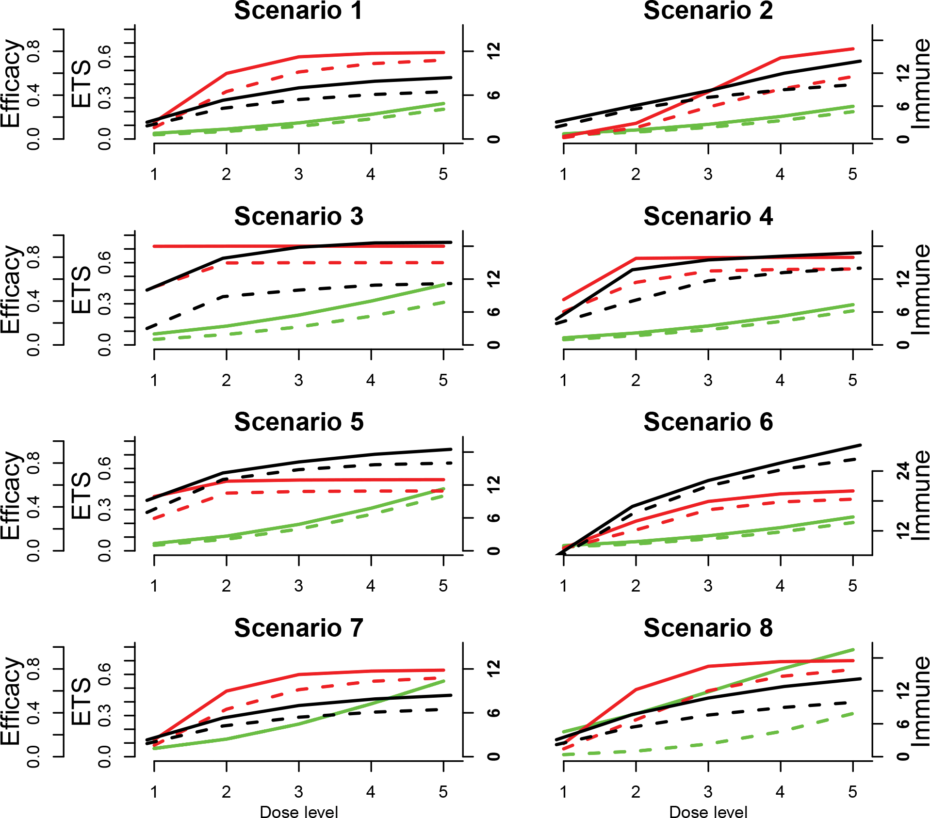
Dose-response curves for the 8 scenarios in the simulation study. The dashed and solid lines are for subgroups S = 0 and S = 1, respectively; and green, red, and black curves are the expected normalized ETS E(X), efficacy p, and the mean immune response μ_Z curves, respectively. The normalized ETS is plotted against the inner y axis on the left; efficacy is plotted against the outer y axis on the left, and the mean immune response is plotted against the right y axis.

Table 1:

True mean immune response μ_Z, efficacy probability p, and expected normalized ETS E(X) for the two subgroups at each dose for the eight scenarios. The numbers in boldface are target doses.

	S=0					S=1
	Scenario 1
μZ	1.8	4.2	5.4	6.1	6.5	2.3	5.3	7	7.9	8.4
p	0.10	0.43	0.61	0.69	0.72	0.15	0.60	0.75	0.78	0.79
E(X)	0.03	0.06	0.09	0.15	0.22	0.04	0.07	0.12	0.18	0.26
	Scenario 2
μZ	2.2	5.4	7.6	9	10	3.1	6	8.8	12	14.2
p	0.01	0.10	0.29	0.45	0.57	0.02	0.14	0.43	0.74	0.82
E(X)	0.03	0.05	0.08	0.13	0.20	0.04	0.07	0.11	0.16	0.24
	Scenario 3
μZ	3	8.8	10	10.9	11.2	10	15.8	17.8	18.6	18.7
p	0.53	0.75	0.75	0.75	0.75	0.90	0.90	0.90	0.90	0.90
E(X)	0.04	0.08	0.13	0.21	0.31	0.08	0.14	0.22	0.32	0.44
	Scenario 4
μZ	3.9	8	11.7	13.2	14	4.7	13.7	15.5	16.2	16.8
p	0.30	0.57	0.67	0.69	0.69	0.41	0.79	0.80	0.80	0.80
E(X)	0.04	0.07	0.11	0.17	0.25	0.05	0.09	0.14	0.21	0.29
	Scenario 5
μZ	7	13	14.8	15.7	16	9.2	14.2	16.2	17.6	18.5
p	0.30	0.53	0.54	0.54	0.55	0.49	0.63	0.65	0.65	0.65
E(X)	0.04	0.08	0.16	0.27	0.40	0.05	0.11	0.19	0.31	0.45
	Scenario 6
μZ	6.4	15.4	21	24.4	26.5	7	16.9	22.1	25.8	29.2
p	0.02	0.19	0.37	0.45	0.47	0.03	0.27	0.45	0.52	0.55
E(X)	0.03	0.05	0.09	0.14	0.21	0.04	0.07	0.11	0.17	0.25
	Scenario 7
μZ	1.8	4.2	5.4	6.1	6.5	2.3	5.3	7	7.9	8.4
p	0.10	0.43	0.61	0.69	0.72	0.15	0.60	0.75	0.78	0.79
E(X)	0.06	0.13	0.24	0.39	0.55	0.06	0.13	0.24	0.39	0.55
	Scenario 8
μZ	2.2	5.4	7.6	9	10	3.1	7.7	10.7	12.8	14.2
p	0.07	0.34	0.60	0.73	0.79	0.12	0.61	0.82	0.87	0.88
E(X)	0.02	0.04	0.09	0.18	0.31	0.18	0.30	0.47	0.64	0.78

Note that in the proposed SIR design, we model the normalized ETS as a quasi-binary outcome rather than directly modeling the ordinal toxicity grades, and as a result, none of the immune response, efficacy, or toxicity data was generated from our proposed models; the latent subgroup membership model (1) is mis-specified with respect to the subgroup partitions we specified; and although the SIR design models toxicity and efficacy independently, these two outcomes were correlated in the simulated data.

We compared the SIR design to the approach that uses the baseline PD-L1 expression to stratify patients (denoted as the baseline design), which is routinely used in practice. We adopted the commonly used cutoff 0.1 so that marker-positive patients were those whose baseline PD-L1 expressions were greater than 0.1. The maker-positive prevalence is 0.53 under this approach and the specified distribution of (M, R). So under the baseline design, the subgroup membership S is known for each patient, and we used the same models (4), (5), and (7) for immune response, efficacy, and toxicity given the known subgroup membership for each patient.

To demonstrate the importance of accounting for the subgroup effect in immunoRT, we also compared the SIR design to the design that did not include the subgroup effects (denoted as the pooled design). Specifically, the immune response, efficacy, and ETS models were given by

$${\mu }_Z\left(d_i\right)=\mu \left(1-\text{exp}\left(-\eta d_i\right)\right)$$

$$\text{logit}(\frac{p_i}{\rho })={\beta }_0+{\beta }_1{Z}_i$$

$$E\left(X_i|d_i\right)=\frac{\text{exp}\left({\gamma }_0+{\gamma }_1{d}_i\right)}{1+\text{exp}\left({\gamma }_0+{\gamma }_1{d}_i\right)}.$$

3.2. Simulation results

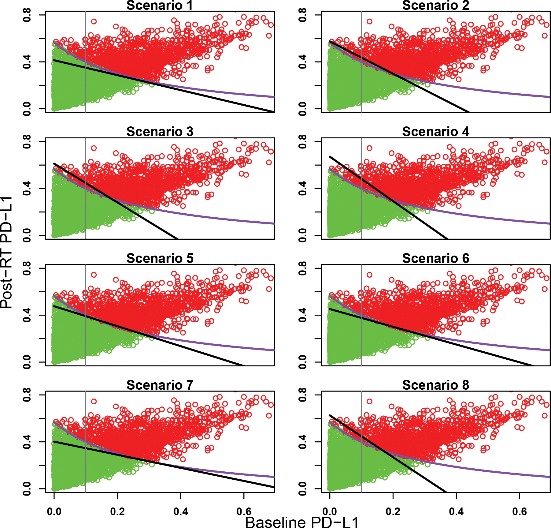
The objective of the design is twofold: (1) to identify subgroups and (2) to determine the optimal dose for each subgroup. Accordingly, we report the results in two ways. To see the capability of the designs to identify subgroups, Figures 3, 4, and 5 display the estimated subgroup partition under the SIR design using the average posterior means of α₁ and α₂ over the 1,000 simulated trials, and the partition under the baseline design, for the eight scenarios under the three partitions. As these figures show, the SIR design was successful in identifying subgroups and the estimated partition boundaries under SIR were much closer to the true partition boundaries than those under the baseline design.

Figure 3:

Estimated partition of the patient population for the eight scenarios under partition 1. The green and red dots represent marker-negative and -positive patients, respectively, randomly selected from the patient population. The blue curve is the true subgroup partition boundary, the black line is the estimated partition boundary from the SIR design, and the gray vertical line is the partition boundary used in the baseline design.

Figure 4:

Estimated partition of the patient population for the eight scenarios under partition 2. The green and red dots represent marker-negative and -positive patients, respectively, randomly selected from the patient population. The purple curve is the true subgroup partition boundary, the black line is the estimated partition boundary from the SIR design, and the gray vertical line is the partition boundary used in the baseline design.

Figure 5:

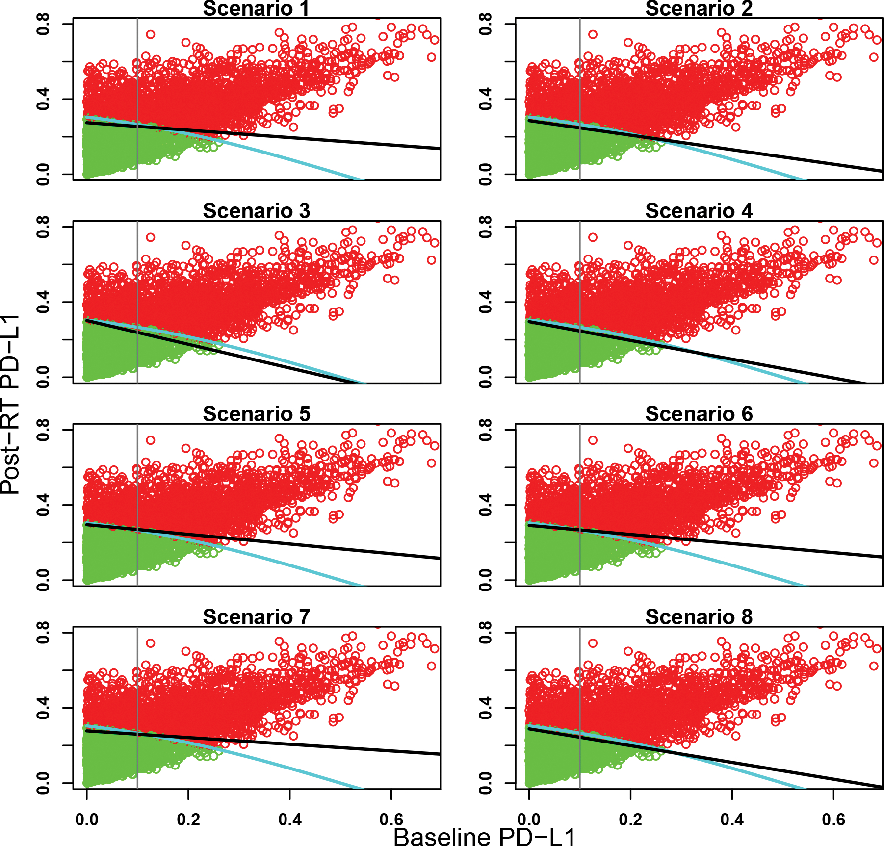
Estimated partition of the patient population for the eight scenarios under partition 3. The green and red dots represent marker-negative and -positive patients, respectively, randomly selected from the patient population. The light blue curve is the true subgroup partition boundary, the black line is the estimated partition boundary from the SIR design, and the gray vertical line is the partition boundary used in the baseline design.

To see the performance of the designs in terms of selecting the optimal dose, Table 2 reports the selection percentage and the average number of patients treated at each dose under the SIR design, the baseline design, and the pooled design, under Partition 1. In the first four scenarios, the optimal dose is different for the two subgroups. The SIR design yielded overall better performance than the other two designs. For example, in scenario 1, all dose levels are safe for both subgroups. The optimal dose is dose level 4 for marker-negative subgroup and dose level 3 for marker-positive subgroup. The percentage of correct optimal dose selection (PCS) was 81.6% and 83.7% for marker-negative and marker-positive subgroups, respectively, under the SIR design; 76% and 50.9% under the baseline design; and 66.2% and 33.8% under the pooled design. Likewise, in scenario 2, the SIR design resulted in much better performance than the other two designs. In scenario 3, the optimal dose is dose level 2 for marker-negative subgroup and dose level 1 for the marker-positive subgroup. The proposed SIR design yielded slightly lower PCS than the other two designs for the marker-negative subgroup (68.5% vs 72.6% and 77.8%), but much higher PCS for the marker-positive subgroup (71% vs 29.4% and 16.6%).

Table 2:

Selection percentage and the average number of patients treated at each dose for the two subgroups under the SIR design, the baseline design that uses the baseline PD-L1 to stratify patients, and the pooled design that ignores subgroup effects, under Partition 1. The numbers in boldface are target doses.

	S=0					S=1
	Scenario 1
Sel % (SIR)	0	0	0.156	0.816	0.027	0	0.02	0.837	0.143	0
# patients	4.9	6.9	7	7.1	7.2	4.8	5.4	5.4	5.6	5.7
Sel % (Baseline)	0	0.001	0.224	0.760	0.015	0	0	0.509	0.488	0.003
# patients	4.7	6.9	7	7.2	7.3	4.6	5.5	5.6	5.6	5.7
Sel % (Pool)	0	0	0.338	0.662	0	0	0	0.338	0.662	0
# patients	5.2	6.8	7	7	7.1	4.2	5.5	5.6	5.7	5.8
	Scenario 2
Sel % (SIR)	0	0	0.002	0.068	0.928	0	0	0.009	0.759	0.232
# patients	1.9	4.2	8.4	9.2	9.3	2	5.5	6.4	6.4	6.7
Sel % (Baseline)	0	0	0.004	0.088	0.902	0	0	0.002	0.221	0.777
# patients	1.9	4	8.1	9.4	9.6	1.7	4.6	6.6	6.9	7.1
Sel % (Pool)	0	0	0	0.103	0.896	0	0	0	0.103	0.896
# patients	1.9	4.7	8.7	8.8	9.1	1.5	3.9	6.9	7.2	7.3
	Scenario 3
Sel % (SIR)	0.309	0.685	0.006	0	0	0.710	0.29	0	0	0
# patients	6.9	6.9	7.3	6.9	5.1	5.7	5.9	6.1	5.4	3.8
Sel % (Baseline)	0.224	0.726	0.05	0	0	0.294	0.699	0.007	0	0
# patients	6.8	6.9	7.2	6.8	5.3	5.6	5.8	5.9	5.5	4.1
Sel % (Pool)	0.166	0.778	0.056	0	0	0.166	0.778	0.056	0	0
# patients	6.9	7.2	7.4	6.8	4.9	5.5	5.8	5.9	5.6	3.9
	Scenario 4
Sel % (SIR)	0.013	0.298	0.664	0.025	0	0.016	0.676	0.308	0	0
# patients	6.4	6.6	6.8	6.8	6.5	5.4	5.3	5.5	5.6	5.2
Sel % (Baseline)	0.007	0.231	0.716	0.046	0	0.008	0.369	0.62	0.003	0
# patients	6.4	6.5	6.9	6.8	6.5	5.3	5.3	5.4	5.5	5.3
Sel % (Pool)	0.003	0.252	0.716	0.029	0	0.003	0.252	0.716	0.029	0
# patients	6.4	6.7	6.9	6.8	6.4	5.2	5.3	5.5	5.5	5.2
	Scenario 5
Sel % (SIR)	0.015	0.801	0.183	0.001	0	0.023	0.919	0.058	0	0
# patients	6.8	7.1	7.7	7	4.4	5.7	5.9	6.2	5.6	3.6
Sel % (Baseline)	0.013	0.762	0.222	0	0	0.015	0.824	0.161	0	0
# patients	6.7	7.1	7.6	6.9	4.7	5.6	5.9	6.1	5.5	3.8
Sel % (Pool)	0.016	0.781	0.203	0	0	0.016	0.781	0.203	0	0
# patients	6.9	7.3	7.7	7	4.3	5.6	6	6.2	5.6	3.4
	Scenario 6
Sel % (SIR)	0	0	0.017	0.743	0.228	0	0	0.07	0.868	0.057
# patients	2.5	5.7	7.8	8.3	8.5	2.9	5.7	6	6	6.3
Sel % (Baseline)	0	0	0.013	0.707	0.244	0	0	0.027	0.801	0.17
# patients	2.5	5.3	7.8	8.2	8.5	2.6	5.3	6.1	6.3	6.5
Sel % (Pool)	0	0	0.023	0.754	0.217	0	0	0.023	0.754	0.217
# patients	2.8	6.1	7.9	8.2	8.2	2.1	4.9	6.4	6.5	6.7
	Scenario 7
Sel % (SIR)	0	0.055	0.806	0.137	0	0	0.12	0.871	0.009	0
# patients	5.6	9.4	9.7	5.8	2.5	5.8	7.2	7.4	4.6	2
Sel % (Baseline)	0	0.089	0.790	0.12	0	0	0.071	0.873	0.056	0
# patients	5.3	9.3	9.5	6.1	2.8	5.2	7.2	7.4	4.8	2.3
Sel % (Pool)	0	0.052	0.880	0.068	0	0	0.052	0.880	0.068	0
# patients	5.9	9.5	9.7	5.7	2.4	4.7	7.8	7.8	4.6	1.9
	Scenario 8
Sel % (SIR)	0	0.004	0.252	0.712	0.031	0.004	0.705	0.291	0	0
# patients	4.7	9.2	9.3	6.6	3.2	5.6	8.6	7.4	3.6	1.7
Sel % (Baseline)	0	0.007	0.477	0.505	0.007	0.002	0.403	0.569	0.023	0
# patients	4.7	9.5	9	6.5	3.5	4.8	8.3	7.3	4.1	2.1
Sel % (Pool)	0	0.127	0.757	0.116	0	0	0.127	0.757	0.116	0
# patients	5.1	10.6	9.8	5.2	2.4	4.1	8.5	8.1	4.3	1.9

In scenarios 5 and 6, the two subgroups have the same optimal dose (dose level 2 for scenario 5 and dose level 4 for scenario 6). For these two scenarios, the SIR design resulted in better or comparable PCS than the other two designs. For example, in scenario 5, the PCS for the two subgroups were 80.1% and 91.9% under SIR, 76.2% and 82.4% under the baseline design, and 78.1% and 78.1% under the pooled design.

In scenarios 7 and 8, the optimal dose is not the dose that reaches the efficacy plateau due to toxicity. For example, in scenario 8, in terms of efficacy alone, dose levels 4 and 3 are the optimal doses for marker-negative and -positive subgroups, respectively. However, dose level 3 is overly toxic for the marker-positive subgroup, so the optimal dose is dose levels 4 and 2 for the two subgroups, respectively. The SIR design yielded higher PCS than the other two designs (71.2% and 70.5% under the SIR design; 50.5% and 40.3% under the baseline design; and 11.6% and 12.7% under the pooled design).

The operating characteristics of the three designs are similar under Partitions 2 and 3 (see Tables S2 and S3 in the Supplementary Materials), which demonstrated the robustness of the SIR design to the subgroup partition.

3.3. Sensitivity Analyses

We have demonstrated that the proposed SIR design is not sensitive to the subgroup partition of the patient population or the mis-specification of the models. We carried out additional sensitivity analyses to assess the robustness of SIR’s performance by using 1) a smaller sample size and 2) less informative prior distributions. Only results under partition 1 are reported in this section.

When the maximum sample size dropped from 60 to 48, the SIR design was still successful in identifying patient subgroups, as shown in Figure S1 in the Supplementary Materials. The selection percentage of the target dose was slightly worse than the original number shown in Table 2, but was still the highest among all doses (see Table 3).

Table 3:

Selection percentage and the average number of patients treated at each dose for the two subgroups under the SIR design when the maximum sample size is 48, under Partition 1. The numbers in boldface are target doses.

	S=0					S=1
	Scenario 1
Sel %	0	0.002	0.218	0.762	0.018	0	0.035	0.801	0.164	0
# patients	4.3	5.3	5.5	5.7	5.9	3.9	4.2	4.4	4.3	4.6
	Scenario 2
Sel %	0	0	0.002	0.08	0.915	0	0	0.014	0.757	0.229
# patients	2	3.8	6.4	7	7.5	1.9	4.3	4.9	4.9	5.2
	Scenario 3
Sel %	0.418	0.574	0.008	0	0	0.693	0.307	0	0	0
# patients	5.4	5.6	6	5.6	4	4.4	4.6	4.9	4.3	3.1
	Scenario 4
Sel %	0.009	0.352	0.595	0.044	0	0.018	0.662	0.319	0.001	0
# patients	5.1	5.2	5.5	5.6	5.3	4.2	4.2	4.4	4.4	4.3
	Scenario 5
Sel %	0.015	0.791	0.188	0.004	0	0.026	0.909	0.065	0	0
# patients	5.3	5.8	6.2	5.6	3.6	4.4	4.7	5	4.4	2.9
	Scenario 6
Sel %	0	0	0.027	0.707	0.26	0	0.001	0.091	0.849	0.059
# patients	2.4	4.6	6.1	6.5	6.9	2.5	4.3	4.8	4.8	4.9
	Scenario 7
Sel %	0	0.057	0.787	0.153	0	0	0.131	0.858	0.011	0
# patients	4.9	7.3	7.7	4.7	2	4.7	5.6	6	3.6	1.6
	Scenario 8
Sel %	0	0.008	0.3	0.66	0.03	0.006	0.526	0.459	0.002	0
# patients	4.5	7.4	7.4	5	2.4	4.8	6.5	5.7	3	1.3

We made all the prior distributions more non-informative. In particular, we assigned β₀ and γ₁ normal priors N(0, 5²) so that the prior scale parameter was twice the previous value. Likewise, we assigned α₁, α₂ truncated normal priors N(0, 5²)I(α_j > 0), j = 1, 2, β₁ truncated normal prior N(0, 5²)I(β₁ > 0), and η truncated normal prior N(0,4.6²)I(η > 0). We assigned a Gamma(0.04, 0.002) prior for μ so that the prior standard deviation was five times the prior mean, i.e., $\tau =5\widehat{\mu }=100$, and an InverseGamma(0.01, 0.01) prior for σ². The operating characteristics of the SIR design are shown in Figure S2 in the Supplementary Materials and Table 4. As Figure S2 and Table 4 show, the performance was similar to the original results in Figure 3 and Table 2, suggesting that the SIR design is not sensitive to prior distributions.

Table 4:

Selection percentage and the average number of patients treated at each dose for the two subgroups under the SIR design under a less informative prior distribution, under Partition 1. The numbers in boldface are target doses.

	S=0					S=1
	Scenario 1
Sel %	0	0	0.195	0.764	0.038	0	0.067	0.854	0.079	0
# patients	4.1	7	7.2	7.4	7.3	4.3	5.5	5.6	5.7	5.8
	Scenario 2
Sel %	0	0	0.001	0.096	0.898	0	0	0.032	0.854	0.114
# patients	1.8	3.7	8.5	9.5	9.6	1.7	5	6.7	6.7	6.8
	Scenario 3
Sel %	0.384	0.612	0.004	0	0	0.896	0.104	0	0	0
# patients	7	7.1	7.5	6.7	4.8	5.9	6	6.1	5.3	3.6
	Scenario 4
Sel %	0.022	0.42	0.554	0.004	0	0.043	0.885	0.072	0	0
# patients	6.4	6.6	6.9	6.8	6.3	5.4	5.3	5.5	5.5	5.1
	Scenario 5
Sel %	0.061	0.831	0.105	0.002	0	0.132	0.843	0.025	0	0
# patients	6.7	7.4	7.9	7	4.1	5.8	6.1	6.3	5.5	3.3
	Scenario 6
Sel %	0	0	0.133	0.709	0.144	0	0.001	0.343	0.624	0.031
# patients	2.4	5.6	8	8.5	8.6	2.6	5.5	6.3	6.3	6.3
	Scenario 7
Sel %	0	0.113	0.745	0.116	0.001	0	0.209	0.783	0.008	0
# patients	4.7	10.4	10.2	5.5	2.2	5.2	8	7.9	4.3	1.7
	Scenario 8
Sel %	0	0.015	0.389	0.582	0.011	0.008	0.677	0.307	0	0
# patients	4.1	10.6	9.9	6	2.6	4.8	9.8	7.5	3.3	1.4

4. Trial application

For illustration, we applied the proposed SIR design to our motivating trial. The trial investigated five doses with a sample size of 60 and a cohort size of 3. Other settings, e.g., lower and upper limits for efficacy and toxicity, equivalence margin for efficacy, probability cutoffs, prior distributions, were all taken to be the same as those used in Section 3. The motivating trial is under the protocol development stage and is pending review from Indiana CTSI. Therefore, this is no real clincial data available. We use hypothetical data to illustrate the SIR design. Patient’s outcomes were generated from scenario 8 in the main simulation setting (Table 1), in which the target dose is dose level 4 for marker-negative patients and dose level 2 for marker-positive patients. We took partition 3 as the two subgroups are balanced in terms of size.

Figure 6 shows the dose allocation and marker subgroups for patients in the 20 cohorts during the trial. The trial started with treating the first cohort of patients at the lowest dose. All three patients experienced grade 0 or 1 toxicity. The mean normalized ETS was lower than the gBOIN escalation boundary, so we escalated the dose to dose level 2. Again all patients in cohort 2 experienced grade 0 or 1 toxicity, and the dose was escalated to dose level 3. For cohort 3 at dose level 3, one patient experienced a grade 2 toxicity and one patient experienced a grade 4 toxicity, so the mean normalized ETS was higher than the gBOIN de-escalation boundary, as a result of which, the dose was de-escalated to dose level 2. Stage I completed after 7 cohorts and we switched to stage II dose finding. In the eighth cohort, two patients were in the negative subgroup and one in the positive subgroup. Their personalized admissible dose sets were (2, 3, 4), (3, 4, 5) and (1, 2, 3). Adaptive randomization resulted in corresponding assigned doses 4, 5, and 2, respectively. As another example, for cohort 15, one patient was in the negative subgroup and two in the positive subgroup. Their personalized admissible dose sets were (2, 3), (1, 2), and (2, 3), with assigned doses 3, 1, and 3. At the end of the trial, the SIR design successfully recommended the target dose for both subgroups, i.e, dose level 4 for negative subgroup and dose level 2 for the positive subgroup.

Figure 6:

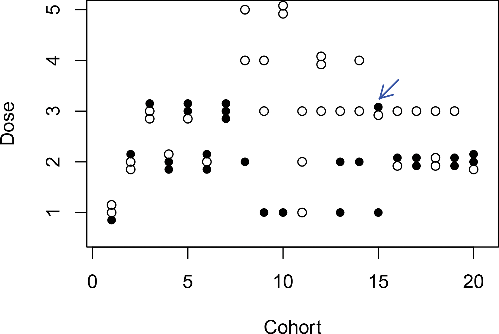
Trial illustration of the SIR design. Solid and empty circle represents a marker-positive and a marker-negative patient, respectively.

5. Discussion

We have proposed the SIR design, a Bayesian phase I/II design to determine patient subgroups and the optimal dose for each subgroup for immunotherapy when adminstered after RT. We construct a latent subgroup membership variable, conditional on which, we jointly model the immune response, toxicity, and efficacy using parsimonious and flexible models to borrow strength across subgroups. We propose a two-stage dose-finding algorithm to assign patients to doses and determine subgroups and subgroup-specific optimal dose at the end of the trial. Simulation studies show that the SIR design has desirable operating characteristics. It reliably identifies subgroups as well as the optimal doses with a large probability. The SIR design requires some pre-determined design parameters. We discuss the choices of them in the Supplementary Materials.

In this article, the binary objective response is used as the efficacy endpoint. In some immunotherapy trials, the ordinal efficacy or the progression-free survival (PFS) time may be a more appropriate efficacy endpoint to quantify the therapeutic effect of the treatment. The SIR design can be extended to those situations in a straightforward way. Specifically, we first construct the latent subgroup membership variable, conditional on which, we jointly model the immune response and the ordinal efficacy (using the proportional odds model) or PFS (using the proportional hazards model). Toxicity is also modeled conditional on the latent subgroup memberships. The SIR design can also be extended to incorporate other patient biomarkers and characteristics to achieve a more personalized medicine. Following most clinical practice, we assume that the dose of RT is pre-fixed. A more challenging yet interesting extension of the proposed design is to relax this assumption and identify the optimal dose-pair for both the radiotherapy and immunotherapy. These are topics of our future research. We wish the proposed design will provide a basis to boost the clinical trial design development for immunoRT.

In our design, we define personalized admissible dose set to increase the ethics of the trial. To illustrate this point, we evaluated the modified version of the design which randomizes a patient to the admissible dose set of his/her estimated subgroup, and compared its operating characteristics to those under the proposed SIR design shown in Section 4 (using the same random seed). The dose allocation and marker subgroups for patients in the 20 cohorts during the trial are shown in Figure S3 in the Supplementary Materials. For the marker-positive subgroup, the true admissible dose set contains dose levels 1 and 2. In stage II, only one marker-positive patient (pointed with an arrow in Figure 6) was assigned to an inadmissible dose under the SIR design, while this number is 7 (pointed with arrows in Figure S3 in the Supplementary Materials) under the subgroup-specific admissible dose set approach. For example, for cohort 14, two patients were in the marker-negative subgroup and one in the marker-positive subgroup. Under the subgroup admissible set approach, the marker-positive patient was mistakenly estimated to belong to the marker-negative subgroup with admissible dose set (3, 4, 5) and randomized to dose level 5.

Data Availability Statement

Data sharing is not applicable to this paper as all data in this article is computer simulated.

References

- [1].Goldstein D, Gordon N, Davidescu M et al. (2017) A Phamacoeconomic Analysis of Personalized Dosing vs Fixed Dosing of Pembrolizumab in Firstline PD-L1-Positive Non-Small Cell Lung Cancer. Journal of the National Cancer Institute, 109(11): djx063. [DOI] [PubMed] [Google Scholar]
- [2].Ingles Garces A, Au L, Mason R, Thomas J, Larkin J (2019), Building on the anti-PD1/PD-L1 backbone: combination immunotherapy for cancer. Expert Opinion on Investigational Drugs, 28: 695–708. [DOI] [PubMed] [Google Scholar]
- [3].Agur Z, Vuk-Pavlovic S (2012) Personalizing immunotherapy Balancing predictability and precision. Oncoimmunotherapy 1, 1169–1171. [DOI] [PMC free article] [PubMed] [Google Scholar]
- [4].Kiyotani K, Toyoshima Y, Nakamura Y (2021) Personalized immunotherapy in cancer precision medicine. Cancer Biology & Medicine 18, 955–965. [DOI] [PMC free article] [PubMed] [Google Scholar]
- [5].Matsumoto A, Nakashima C, Kimura S, Sueoka E, Aragane N (2021) ALDH2 polymorphism rs671 is a predictor of PD-1/PD-L1 inhibitor efficacy against thoracic malignancies. BMC Cancer 21:584. [DOI] [PMC free article] [PubMed] [Google Scholar]
- [6].Topalian S, Hodi F, Brahmer J, et al. (2012), Safety, Activity, and Immune Correlates of Anti-PD-1 Antibody in Cancer. The New England Journal of Medicine, 366: 2443–2454. [DOI] [PMC free article] [PubMed] [Google Scholar]
- [7].Manhoney KM, Atkins MB (2014), Prognostic and predictive markers for the new immunotherapies. Oncology, 28: 39–48. [PubMed] [Google Scholar]
- [8].Borghaei H, Paz-Ares L, Horn L, et al. (2015), Nivolumab versus docetaxel in advanced nonsquamous non-small-cell lung cancer. The New England Journal of Medicine, 373: 1627–39. [DOI] [PMC free article] [PubMed] [Google Scholar]
- [9].Garon EB, Rizvi NA, Hui R, et al. (2015), Pembrolizumab for the treatment of non-small-cell lung cancer. The New England Journal of Medicine, 372: 2018–28. [DOI] [PubMed] [Google Scholar]
- [10].Larkin J, Chiarion-Sileni V, Gonzles R, et al. (2015), Combined nivolumab and ipilimumab or monotherapy in untreated melanoma. The New England Journal of Medicine, 373: 23–34. [DOI] [PMC free article] [PubMed] [Google Scholar]
- [11].Aguiar P, Santoro S, Tadokoro H, et al. (2016), The role of PD-L1 expression as a predictive biomarker in advanced non-small-cell lung cancer: a network meta-analysis. Immunotherapy, 8, 479–488. [DOI] [PubMed] [Google Scholar]
- [12].Ribas A, Wolchok J (2018) Cancer immunotherapy using checkpoint blockade. Science 359, 1350–1355. [DOI] [PMC free article] [PubMed] [Google Scholar]
- [13].Lhuillier C, Vanpouille-Box C, Galluzzi L, Formenti S, Demaria S (2018) Emerging biomarkers for the combination of radiotherapy and immune checkpoint blockers. Seminars in Cancer Biology 52, 125–134. [DOI] [PMC free article] [PubMed] [Google Scholar]
- [14].Weichselbaum R, Liang H, Deng L, Fu Y (2017) Radiotherapy and immunotherapy: a beneficial liaison. Nature Review Clinical Oncology 14, 365–379. [DOI] [PubMed] [Google Scholar]
- [15].Turgeon G, Weichhardt A, Azad A, Solomon B, Siva S (2019) Radiotherapy and immunotherapy: a synergistic effect in cancer care. The Medical Journal of Australia 210, 47–53. [DOI] [PubMed] [Google Scholar]
- [16].Sato H, Okonogi N, Nakano T (2020) Rationale of combination of anti-PD-1/PD-L1 antibody therapy and radiotherapy for cancer treatment. International Journal of Clinical Oncology 25, 801–809. [DOI] [PMC free article] [PubMed] [Google Scholar]
- [17].Kong Y, Ma Y, Zhao X, Pan J, Xu Z, Zhang L (2021) Optimizing the treatment schedule of radiotherapy combined with anti-PD-1/PD-L1 immunotherapy in metastatic cancers. Frontiers in Oncology 11: 638873. [DOI] [PMC free article] [PubMed] [Google Scholar]
- [18].Harris T, Kipkiss E, Borzillary S, et al. (2008) Radiotherapy augments the immune response to prostate cancer in a time-dependent manner. Prostate 68, 1319–1329. [DOI] [PMC free article] [PubMed] [Google Scholar]
- [19].Twyman-Saint, et al. (2015) Radiation and Dual Checkpoint Blockade Activates Non-Redundant Immune Mechanisms in Cancer. Nature 520, 373–377. [DOI] [PMC free article] [PubMed] [Google Scholar]
- [20].Teng F, Kong L, Meng X, Yang J, Yu J (2015) Radiotherapy combined with immune checkpoint blockade immunotherapy: achievements and challenges. The Medical Journal of Australia 210, 47–53. [DOI] [PubMed] [Google Scholar]
- [21].Antonia S, Villegas A, Daniel D, et al. (2018) Overall Survival with Durvalumab after Chemoradiotherapy in Stage III NSCLC. Engl J Med 379, 2342–2350. [DOI] [PubMed] [Google Scholar]
- [22].Brahmer J, Govindan R, Anders R, et al. (2018) The society for immunotherapy of cancer consensus statement on immunotherapy for the treatment non-small cell lung cancer (NSCLC). Journal for Immunotherapy of Cancer 6, 75. [DOI] [PMC free article] [PubMed] [Google Scholar]
- [23].Yoneda K, Kuwata T, Kanayama M, Mori M et al. (2019) Alteration in tumoural PD-L1 expression and stromal CD8-positive tumour-infiltrating lymphocytes after concurrent chemo-radiotherapy for non-small cell lung cancer. British Journal of Cancer 121, 490–496. [DOI] [PMC free article] [PubMed] [Google Scholar]
- [24].Arina A, Beckett M, Fernandez C et al. (2019) Tumor-reprogrammed resident T cells resist radiation to control tumors. Nature Communications 10, 3959. [DOI] [PMC free article] [PubMed] [Google Scholar]
- [25].Yuan Z, Chappell R, Bailey H (2007) The continual reassessment method for multiple toxicity grades: a Bayesian quasi-likelihood approach. Biometrics, 63, 173–179. [DOI] [PubMed] [Google Scholar]
- [26].Lee J, Thall P, Rezvani K (2019), Optimizing natural killer cell doses for heterogenous cancer patients on the basis of multiple event times. Journal of the Royal Statistical Society, Series C, 68: 461–474. [DOI] [PMC free article] [PubMed] [Google Scholar]
- [27].Lee J, Thall P, Msaouel P (2021), Precision Bayesian phase I-II dose-finding based on utilities tailored to prognostic subgroups. Statistics in Medicine, DOI: 10.1002/sim.9120. [DOI] [PMC free article] [PubMed] [Google Scholar]
- [28].Guo B, Zang Y (2022a) BIPSE: A Biomarker-based Phase I/II Design for Immunotherapy Trials with Progression-free Survival Endpoint. Statistics in Medicine In Press. [DOI] [PMC free article] [PubMed] [Google Scholar]
- [29].Guo B, Zang Y (2022b) A Bayesian Phase I/II Biomarker-based Design for Identifying Subgroup-Speci c Optimal Dose for Immunotherapy. Statistical Methods in Medical Research In Press. [DOI] [PMC free article] [PubMed] [Google Scholar]
- [30].Spiegelhalter D, Best N, Carlin B, van der Linde A (2002) Bayesian measures of model complexity and fit (with discussion). Journal of the Royal Statistical Society, Series B, 64, 583–639. [Google Scholar]
- [31].Papke L and Wooldridge J (1996) Econometric methods for fractional response variables with an application to 401(k) plan participation rates. Journal of Applied Econometrics, 11, 619–632. [Google Scholar]
- [32].Cai C, Yuan Y, Ji Y (2014) A Bayesian dose finding design for oncology clinical trials of combinational biological agents. Applied Statistics 63, 159–173. [DOI] [PMC free article] [PubMed] [Google Scholar]
- [33].Gelman A, Jakulin A, Pittau MG, Su YS (2008) A weakly informative default prior distribution for logistic and other regression models. The Annals of Applied Statistics, 2: 1360–1383. [Google Scholar]
- [34].Gelfand A, Smith A (1990) Sampling-Based Approaches to Calculating Marginal Densities. Journal of the American Statistical Association, 85, 398–409. [Google Scholar]
- [35].Geman S, Geman D (1984) Stochastic Relaxation, Gibbs distributions, and the Bayesian restoration of images. IEEE Transactions on Pattern Analysis and Machine Intelligence, 6, 721–741. [DOI] [PubMed] [Google Scholar]
- [36].Mu R, Yuan Y, Xu J, Mandrekar S, Yin J (2019) gBOIN: a unified model-assisted phase I trial design accounting for toxicity grades, and binary or continuous end points. Applied Statistics, 68, 289–308. [Google Scholar]
- [37].Chen Q, Fu Y, Yue Q, Wu Q, Tang Y, et al. (2019) Distribution of PD-L1 expression and its relationship with clinicopathological variables: an audit from 1071 cases of surgically resected non-small cell lung cancer. International Journal of Clinical and Experimental Pathology, 12, 774–786. [PMC free article] [PubMed] [Google Scholar]
- [38].Xu S, Tian M, Zhang X, Qi C, Song C, et al. (2020) Distribution of PD-L1 expression level across major tumor types. Journal of Clinical Oncology, 38, DOI: 10.1200/JCO.2020.38.15suppl.e15176. [DOI] [Google Scholar]
Associated Data
This section collects any data citations, data availability statements, or supplementary materials included in this article.
Supplementary Materials