Optimization of blood pressure measurement practices for pharmacodynamic analyses of tyrosine‐kinase inhibitors

Abstract

Blood pressure measurements form a critical component of adverse event monitoring for tyrosine kinase inhibitors, but might also serve as a biomarker for dose titrations. This study explored the impact of various sources of within‐individual variation on blood pressure readings to improve measurement practices and evaluated the utility for individual‐ and population‐level dose selection. A pharmacokinetic–pharmacodynamic modeling framework was created to describe circadian blood pressure changes, inter‐ and intra‐day variability, changes from dipper to non‐dipper profiles, and the relationship between drug exposure and blood pressure changes over time. The framework was used to quantitatively evaluate the influence of physiological and pharmacological aspects on blood pressure measurements, as well as to compare measurement techniques, including office‐based, home‐based, and ambulatory 24‐h blood pressure readings. Circadian changes, as well as random intra‐day and inter‐day variability, were found to be the largest sources of within‐individual variation in blood pressure. Office‐based and ambulatory 24‐h measurements gave rise to potential bias (>5 mmHg), which was mitigated by model‐based estimations. Our findings suggest that 5–8 consecutive, home‐based, measurements taken at a consistent time around noon, or alternatively within a limited time frame (e.g., 8.00 a.m. to 12.00 p.m. or 12.00 p.m. to 5.00 p.m.), will give rise to the most consistent blood pressure estimates. Blood pressure measurements likely do not represent a sufficiently accurate method for individual‐level dose selection, but may be valuable for population‐level dose identification. A user‐friendly tool has been made available to allow for interactive blood pressure simulations and estimations for the investigated scenarios.

Study Highlights.

• WHAT IS THE CURRENT KNOWLEDGE ON THE TOPIC?

Blood pressure readings form a critical component of adverse event monitoring for tyrosine kinase inhibitors (TKIs), but have additionally gained attention as a biomarker for individual‐level dose titrations due to their population‐level relation with treatment outcome.

• WHAT QUESTION DID THIS STUDY ADDRESS?

Proposing an initial population‐level dose and finding the best individual‐level dose represent two very different undertakings. Due to the dynamic nature of blood pressure and issues related to measurement practices, measured values may differ from the true baseline value, potentially giving rise to inaccurate dose recommendations. The current study quantifies both physiological and clinical sources of measurement error to provide recommendations for blood pressure measurements and their use for dose titration.

• WHAT DOES THIS STUDY ADD TO OUR KNOWLEDGE?

The current work confirms the utility of repeated, home‐based measures on similar samplings times to increase the consistency and accuracy of blood pressure readings.

• HOW MIGHT THIS CHANGE CLINICAL PHARMACOLOGY OR TRANSLATIONAL SCIENCE?

These results could be utilized for population‐level dose optimization in clinical trials, as a potential base for dose selection or dose translation between populations. However, the practicality of our suggested method for individual‐level dose optimization for clinical practice is limited due to issues related to fear, compliance, and limited time for repeated measures to take place, in addition to dynamic changes when drug holidays schedules of TKIs are used.

INTRODUCTION

Tyrosine kinase inhibitors (TKIs) represent a group of targeted therapies that form an important component of both initial (first‐line) and subsequent (second‐line) therapies for a wide variety of cancers. ¹ By April 2021, 72 kinase inhibitors had received approval for cancer applications by the European Medicines Agency (EMA), whereas 89 TKIs had received market authorization for oncological purposes by the US Food and Drug Administration (FDA). ² For many of these TKIs, large variability in dose–response and dose–toxicity have been observed, giving rise to either suboptimal treatment efficacy or treatment‐related toxicities. ¹ , ³ , ⁴ It is therefore increasingly appreciated that dose individualization based on biomarkers can be used to reduce variability in outcomes and maximize treatment benefit.

Suggested approaches for dose individualization include those based on pharmacokinetic biomarkers, such as the a priori genetic cytochrome P450 (CYP) profiling ⁵ , ⁶ and a posteriori therapeutic drug monitoring (TDM) of drug plasma concentration, ¹ , ⁷ or biomarkers, based on soluble vascular endothelial growth factor receptor (sVEGFR)‐3, ⁸ neutrophil count,⁹ or diastolic blood pressure. ⁹ , ¹⁰ , ¹¹ Of these biomarkers, blood pressure is the least invasive, which might facilitate clinical implementation and repeated measurements. The TKIs targeting VEGF are most often associated with an increase in (diastolic) blood pressure, particularly axitinib, sunitinib, and sorafenib. ¹² Given the frequent occurrence of hypertension following anti‐VEGF TKI initiation, blood pressure monitoring already represents an important component of patient management for these drugs. ¹² , ¹³ , ¹⁴

Previous efforts have evaluated blood pressure as a pharmacodynamic biomarker for dose titration, both as an absolute (i.e., diastolic ≤90 mmHg) ¹³ and relative threshold value (i.e., diastolic ≤7.5% increase). ¹⁵ , ¹⁶ In a prospective randomized trial of patients with metastatic renal cell carcinoma (mRCC) in patients with diastolic blood pressure ≤95 mmHg, axitinib titration (n = 56) versus standard dosing (n = 56) did not yield a higher progression‐free survival, ¹⁷ even though a previous retrospective analysis suggested otherwise. ¹⁰ , ¹⁸ A similar evaluation of axitinib in mRCC found dynamic blood pressure changes to exhibit high measurement accuracy. ¹¹ , ¹⁶ However, a study of sunitinib in gastrointestinal stromal tumors found relative blood pressure changes to have high measurement error that obscure informed dose decisions. ⁹ , ¹⁹ This issue of ‘measurement noise’ in the use of blood pressure as a biomarker for TKI therapy has been coined a decade ago, but efforts to reduce the various sources of noise have been lacking. ²⁰

Deterministic (i.e., fixed/structural) influences on blood pressure can occur due to periodic hormonal and physiological changes giving rise to a circadian rhythm ²¹ (Figure 1). Under normal physiological circumstances, blood pressure will exhibit a nighttime dip, followed by a morning surge known as the ‘dipper profile’. ²¹ Under a ‘non‐dipper profile’, blood pressure remains high at night (≤10% decrease from daytime average) due to pathophysiological vascular rearrangements or medications. ²¹ Indeed, in several instances it has been observed that TKIs might reduce the magnitude of the nighttime dip, giving rise to the ‘non‐dipper profile’. ²²

FIGURE 1.

Within‐individual blood pressure variation. Diastolic blood pressure for one individual patient, including the underlying baseline value (gray dashed line), true value including long‐term fluctuations (i.e., inter‐day variability [black lines]), and measurements deviating from the true blood pressure value due to short‐term fluctuations (i.e., intra‐day variability [black dots]).

Stochastic (i.e., random/unpredictable) differences in blood pressure can arise from unexplained inter‐ or intra‐individual variability (Figure 1). From a clinical perspective, inter‐day fluctuations have been classified as unexplained long‐term fluctuations (>24 h), whereas intra‐day variability would represent unexplained short‐term fluctuations (<24 h). ²³

Different measurement approaches, such as office versus home measurements and single versus 24‐h ambulatory blood pressure measurements, ¹³ can result in biases due to white‐coat hypertension in office‐based measurements ²⁴ or non‐randomly missing data samples during ambulatory measurements. ²⁵

A quantitative understanding of how each of the abovementioned influencers affects blood pressure accuracy will give rise to improved measurement recommendation and possibly reduced measurement noise, which could increase the utility for dosing practices. Nonlinear mixed‐effects models have been developed as statistical tools that incorporate biological features to understand variability in pharmacological and physiological endpoints. ²⁶ , ²⁷ Previous efforts have given rise to blood pressure models that capture the various deterministic and stochastic aspects related to blood pressure changes over time. ²⁸ , ²⁹ , ³⁰ , ³¹ , ³² , ³³ , ³⁴ In addition, multiple exposure–response models have become available, linking drug TKI exposure to longitudinal changes in blood pressure. ⁹ , ¹¹ , ³⁴ , ³⁵ , ³⁶ However, adaptation of these models requires a degree of expertise and clinical implementation might be hampered.

In consideration of the abovementioned issues related to measurement noise, the aim of the study was to adapt a model‐based approach to (1) determine if blood pressure can be used for individual‐level dosing decisions for anti‐VEGF TKIs and (2) evaluate methods to reduce this measurement noise to optimize accuracy for dosing decisions (both at population and individual level).

METHODS

Model selection and biomarker evaluation

Blood pressure models were searched on PubMed during April 2022, using the terms “blood pressure AND (NONMEM OR MONOLIX OR ADAPT) OR (non‐linear mixed effects) AND circadian”. Models linking TKI exposure to changes in blood pressure were searched by “(((PKPD[Title/Abstract]) OR (PK/PD[Title/Abstract]) OR (exposure response[Title/Abstract])) AND (blood pressure)) AND (kinase inhibitor)”. Backward (and forward) citations were used to identify supplementary models. Additionally, abstracts from the annual Population Approach Group in Europe (PAGE), American Conference on Pharmacometrics (ACoP), World Conference on Pharmacometrics (WCoP), and Population Approach Group in Australia and New Zealand (PAGANZ) meetings were searched.

The selection for the blood pressure model to be used in the simulations was based on the following criteria with decreasing weight: capacity to describe (1) inter‐day variability, (2) diastolic blood pressure changes, and (3) blood pressure in Caucasian individuals.

Simulations of physiological influencers

The selected models were translated to the R‐based package mrgsolve (version 0.8.10) with the corresponding parameter estimates. A virtual population was generated to emulate real‐life patients. Dichotomous covariates reported in the model were randomly selected based on probability distributions for: age >60 years (0.0226/0.9774), non‐Caucasian race (0.38/0.62), and smoker (0.12/0.88; yes/no), following a reported population distribution. ³⁷

Diastolic and systolic measure were lowered to 70 mmHg diastolic and 120 mmHg systolic, respectively, ²¹ to account for the relatively low occurrence of primary hypertension at start of therapy. All selected models were linked to describe the relationship between TKI dose, concentration, and blood pressure changes. ¹⁸ , ³⁰ , ³⁴

Subsequently, simulations were performed to assess the impact of the following influencers on measurement consistency:

1. Circadian rhythm (deterministic effect).

2. Inter‐day variability (stochastic effect).

3. Intra‐day variability (stochastic effect).

4. Dipper to non‐dipper changes (deterministic effect).

5. Inaccurate documentation of drug intake time (deterministic effect).

Diastolic blood pressure was selected as the simulated variable, because of its current use in dose titration and in pharmacodynamic biomarker studies. ⁹ , ¹⁰ , ¹¹ , ¹⁸ The consistency in blood pressure between two measurements within an individual (BP _i (t ₁) and BP _i (t ₂)) was initially assessed based on random absolute difference (Equation 1), and the absolute difference between the maximum measured blood pressure and the minimum measured blood pressure within individuals (BP _i [max] and BP _i [min]). A summary measure of the latter was the population mean maximum variation (MMV) (Equation 2).

$$\mathrm{\Delta BP}={\mathrm{BP}}_i\left(t1\right)-{\mathrm{BP}}_i\left(t2\right)$$ (1)

$$\mathrm{MMV}={\sum }_{i=1}^n\frac{{\mathrm{BP}}_i\left(\max \right)-{\mathrm{BP}}_i\left(\min \right)}{n}$$ (2)

Each physiological source of measurement noise was investigated separately to evaluate the impact on the MMV. In order to isolate the impact of each investigated influencer, other sources of intra‐individual biomarker fluctuations were omitted during the corresponding simulations. For the investigations of circadian rhythm (I), the influence of inter‐ and intra‐day variability was fixed at 0. Recordings were performed at random timepoints within a defined time window to mimic a realistic scenario (e.g., 8.00 a.m. to 5.00 p.m. and 7.00 a.m. to 10.00 p.m., respectively). Likewise, investigations of the impact of inter‐ and intra‐day variability (II–III) were performed at the same time points of the day, to avoid any influences from circadian changes. Here, the recordings were performed at the following timepoints to mimic realistic scenarios: 7.00 a.m., 8.00 a.m., 12.00 p.m., 5.00 p.m. and 10.00 p.m.

Model adjustments were made to mimic the potential switch from dipper profile to non‐dipper profile (IV) under treatment with TKIs. For this purpose, population parameter changes between dipper and non‐dippers were derived from a previous investigation ³⁸ and translated into the blood pressure model. A 50% reduction in circadian amplitude was introduced with an associated increase in baseline blood pressure in order to account for non‐dippers, resulting in a reduced nighttime dip with a preserved morning peak. ³⁸ Measurement consistencies were here determined by comparing the dipper profile with non‐dipper profile within each individual.

Under steady‐state conditions, the time of TKI dose intake was increasingly shifted away from the baseline afternoon dosing time of 12.00 p.m., in increments of 1 h, to explore the impact of inaccurate dose intake or documentation (V). Blood pressure was then assumed to be measured the following afternoon (i.e., 24‐h thereafter). Changes in blood pressure values were compared to changes if the dose would have been taken at the default time of 12.00 p.m. (i.e., noon) within each individual.

Simulations of measurement practices

Following a similar approach, the limitations of different measurement practices were evaluated. In these simulations, all sources of measurement noise were added simultaneously to represent a real‐life scenario. The investigated conditions were:

1. Office‐based measurements.

2. Home‐based measurements.

3. 24‐h ambulatory blood pressure measurements.

For the office‐based scenario (I), an additional parameter was added to the model to account for the occurrence of white‐coat hypertension. The values for this parameter derived from a previous comparison between ambulatory blood pressure monitoring and office‐based measurements. ³⁹ For each patient, a parameter representing white‐coat hypertension was drawn from a given distribution (i.e., dBP 6.2 ± 5.57 SD). ³⁹ Desensitization to white‐coat hypertension was explored by gradual decrease of the sampled white‐coat hypertension value to 50% between visit 1 and 4 (e.g., 12.5% per visit), as described in a previous study. ²⁴

Home‐based measurements (scenario IIa) were simulated following the same procedure, but without the inclusion of white‐coat hypertension. Additionally, the scenario (IIb) of multiple measurements (three samples; ‘rich sampling’) on a single day (i.e., the optimized time points around 11.00 a.m. and 12.00 p.m.) was simulated.

Following the information derived from the previous simulations (I–II), measurement times that provided the lowest degree of within‐individual variability were used for the office‐ and home‐based measurements. For both the office‐ and home‐based measurements, recordings were performed once per day using the previously optimized timepoint. The accuracies of office‐ and home‐based measurements were thereafter evaluated using datasets with an increasing number of daily measurements to compute the mean (e.g., values on days 1–10). All simulated measurement observations contained both inter‐ and intra‐day variability. The mean of all measured values for each individual up to the last sample time was then compared to the ‘true’ individual blood pressure (BP_true) at the sampled time (i.e., simulated blood pressure without inter‐ and intra‐day variability):

$$\begin{array}{c}{\text{Accuracy}}_{\text{OFFICE}/\text{HOME measurements}}\hfill \\ =\left({\mathrm{BP}}_{\text{mean},\text{measured}}-{\mathrm{BP}}_{\text{true}}\right)/{\mathrm{BP}}_{\text{true}}\times 100\%.\hfill \end{array}$$ (3)

In the 24‐h ambulatory measurement scenario (III), blood pressure values were simulated to be recorded every 15 min between 12.00 a.m. and 11.59 p.m. To account for missing values, various percentages (10%–90%) of measurements were randomly removed from the dataset. This process was repeated for measurements made solely during daytime (7.00 a.m. and 10.00 p.m.) to evaluate the possibility of measurement bias due to higher waketime activity and related measurement errors. Each simulated sample contained both inter‐ and intra‐day variability. Final blood pressure accuracy was determined by comparing the average of all measured blood pressure during 24 h for one individual (ranging from 10 to 96 measurements during a day) with the ‘true’ average blood pressure (BP_{mean 24 h,true}, i.e., the simulated average 24‐h blood pressure without inter‐ and intra‐day variability):

$$\begin{array}{c}{\text{Accuracy}}_{\text{AMBULATORY measurements}}=\left({\mathrm{BP}}_{\text{mean}24\mathrm{h},\text{measured}}\right.\hfill \\ \left.-{\mathrm{BP}}_{\text{mean}24\mathrm{h},\text{true}}\right)/{\mathrm{BP}}_{\text{mean}24\mathrm{h},\text{true}}\times 100\%.\hfill \end{array}$$ (4)

Model‐based individual estimations for different measurement practices

A model‐guided individualization approach was evaluated following a simulation‐estimation‐prediction procedure in NONMEM (version 7.4). The previously simulated individual blood pressure measurements, representing either office‐based, home‐based (rich and poor sampling) measurements, or 24‐h ambulatory blood pressure measurements, were used for this purpose. All datapoints included both inter‐ and intra‐day variability. The selected blood pressure model and population parameters, including white‐coat hypertension where applicable, was applied to estimate individual parameter values based on the simulated data (Table S1). Similar to the direct clinical measurement scenario, varying numbers of measurements were explored to evaluate the impact of number of recordings on the accuracy in the parameter estimates. For office‐based measurements two scenarios were evaluated:

1. A scenario with (biased) model‐based estimations, where the model was not informed about presence and degree of white‐coat hypertension.

2. A scenario without (non‐biased) model‐based estimations were evaluated, where the model was informed about presence and degree of white‐coat hypertension.

Individual parameters were obtained through Bayesian feedback using the original population and residual error parameters to inform the model. Estimated parameters representing the individual difference from the typical patient (${\eta }_i$) were subsequently used to predict individual blood pressure profiles (IPREDs). The individual predicted blood pressure profiles were then compared to the simulated (‘true’) individual profiles to evaluate the difference between ‘true’ and ‘estimated’ blood pressure. The comparison was made between the underlying profiles without inter‐ and intra‐day variability:

$$\begin{array}{c}{\text{Accuracy}}_{\text{home}/\text{office},\text{estimations}}=\left({\mathrm{BP}}_{\text{mean},\text{estimated}}-{\mathrm{BP}}_{\text{true}}\right)/\hfill \\ {\mathrm{BP}}_{\text{true}}\times 100\%.\hfill \end{array}$$ (5)

$$\begin{array}{c}{\text{Accuracy}}_{\text{ambulatory},\text{estimations}}=\left({\mathrm{BP}}_{\text{mean}24\mathrm{h},\text{estimated}}\right.\hfill \\ \left.-{\mathrm{BP}}_{\text{mean}24\mathrm{h},\text{true}}\right)/{\mathrm{BP}}_{\text{mean}24\mathrm{h},\text{true}}\times 100\%.\hfill \end{array}$$ (6)

For both the home‐ and office‐based estimations, an intermediate step was performed to evaluate the influence of sampling time on model predictions. Selection of the most accurate sampling time was based on the 24‐h time point that gave rise to the highest accuracy.

Interactive tool for model‐based simulations and estimations

An interactive R‐based app was created to facilitate data simulation, estimation, and visualization following the various scenarios. The user‐friendly interface was constructed using the dplyr (Version 1.0.5), ggplot (Version 3.3.3), shiny (Version 1.6.0), and shinythemes (Version 1.2.0) packages. ⁴⁰ , ⁴¹ The tool was adjusted to allow for the estimation of individual parameter estimates, based on user‐provided data input. The objective function of residual sum of squares ⁴² was minimized to derive individual parameter estimates:

$${\mathrm{OBJ}}_{\text{sqwres}}={\sum }_{j=1}^p\left[\log {\left({\sigma }_{\mathit{ij}}\right)}^2+\frac{{\left({\widehat{\mathrm{BP}}}_{\mathit{ij}}-{\mathrm{BP}}_{\mathit{ij}}\right)}^2}{{{\sigma }_{\mathit{ij}}}^2}\right]+{\stackrel{⃑}{\eta }}_i^T{\Omega }^{-1}{\stackrel{⃑}{\eta }}_i$$ (7)

where BP _ij denotes the jth blood pressure observation of the ith individual, $\sigma$ the residual unexplained variability, $\eta$inter‐individual random variability, and $\Omega$ represents the covariance matrix for inter‐individual variability.

RESULTS

Model selection

Seven circadian blood pressure models ²⁸ , ²⁹ , ³⁰ , ³¹ , ³² , ³³ , ³⁴ and four exposure–response models ⁹ , ¹¹ , ³⁴ , ³⁵ were identified. The model by Trocóniz et al. ³⁰ was selected (Table S1) over other identified circadian models for different reasons (Table S2). This model captures blood pressure changes (BP) (t) by inclusion of two closed‐form cosine equations:

$$\begin{array}{c}\mathrm{BP}\left(t\right)={\kappa }_{1\mathrm{d}}+{\theta }_1\times \exp \left({\eta }_1\right)\times \hfill \\ \left[1+{\sum }_{n=1}^n{\theta }_{2\mathrm{i}}\times \left(1+{\eta }_2\right)\times \cos \left(\frac{\mathrm{i}\times \pi \times \left(t+{\eta }_3+{\kappa }_{2d}\right)}{12}-{\theta }_{2i+1}\right)\right]\hfill \end{array}$$

where $\theta$ accounts for the fixed‐effect parameters, where $\eta$ (inter‐individual variability) and $\mathrm{\kappa }$ (inter‐day variability) represent the random effect parameters on blood pressure baseline, amplitude, and peak time.

An exposure–response model of axitinib ³⁴ was selected, as it represents the TKI with the shortest half‐life. ⁷ The accompanying pharmacokinetic model by Rini et al. ¹⁸ was selected to characterize the exposure in the model framework.

Impact of physiological influencers

Of the 24 simulated scenarios, circadian changes were shown to be the largest source of blood pressure variations between two measurements within one individual, with a MMV of 17.3 mmHg on a population level (Figure 2a). This variation could largely be reduced, however, by sampling either in the morning (08.00 a.m. to 12.00 p.m.; MMV = 3.9 mmHg) or in the afternoon office‐hour (12.00 p.m. to 5.00 p.m.; MMV = 3.4 mmHg) windows.

FIGURE 2.

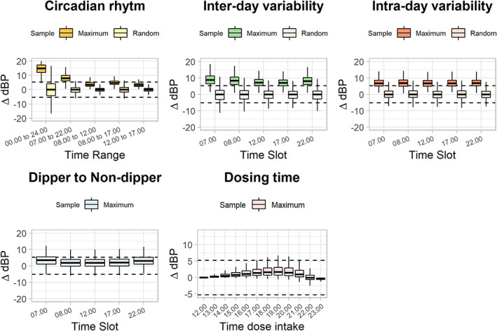
Influence of physiological processes on absolute differences in diastolic blood pressure measurements between two measurements occasions. In each plot, the ±5.25 mmHg dashed lines represent the proposed blood pressure threshold at which a typical individual might require dose changes under a tyrosine kinase inhibitor (TKI) (i.e., 7.5% of 70 mmHg). Maximum boxes represent the maximum difference between two observation times within an individual over 10 measurement occasions, random boxes represent the difference between two random times of observation within an individual. Each box illustrates the 25th and 75th percentiles with the population median value. Whiskers are the 2.5th and 97.5th percentiles, respectively. ΔBP = Consistency: absolute difference between two blood pressure measurements.

Two additional large sources of individual diastolic blood pressure fluctuations were inter‐day variability (MMV = 8.1 mmHg) and intra‐day variability (MMV = 6.9 mmHg; Figure 2b,c). Although both were more evenly spread throughout the day, the influence of inter‐day variability was the lowest at noon (12.00 p.m.; MMV = 7.3 mmHg vs. day average; MMV = 8.1 mmHg).

A more systematic bias in blood pressure deviation was seen for the switch from dipper‐to‐non‐dipper (MMV = 2.4 mmHg), where diastolic blood pressure was almost consistently larger under the non‐dipper profile compared to the dipper profile, or for inaccurate dose intake documentation (MMV = 1.2 mmHg; Figure 2d,e). Besides the potential bias, the measurement inaccuracy appears to be relatively low compared to the other diastolic blood pressure influencers.

Based on the above findings of circadian changes, inter‐ and intra‐day variability, and dipper‐ to non‐dipper changes, the optimal measurement time point and measurement time‐windows for blood pressure measurements were fixed at 12.00 p.m. and 12.00 p.m. to 5.00 p.m., respectively.

Impact of measurement practices

The accuracy of diastolic blood pressure measurements under the investigated measurement methods are summarized in Figure 3. Both white‐coat hypertension and missing daytime measurements gave rise to bias in the estimated blood pressure values.

FIGURE 3.

Influence of measurement practices on the accuracy (% from true mean dBP) of diastolic blood pressure measurements. Multiple single measurements. Single blood pressure measurement taken at an increasing number of separate occasions (days 1–10; 12.00 p.m.). Darker boxes represent the office‐based scenario, with potential white‐coat hypertension. Office with no bias represents the scenario where model‐based estimations are informed about white‐coat hypertension. Lighter boxes represent the home‐based scenario, without white‐coat hypertension. Ambulatory 24‐h measurements. 24‐h ambulatory blood pressure measurements during a single day, with an increasing percentage of datapoints included (measurement can occur every 15 min). Dark boxes represent the scenario where datapoints are randomly missing during awake time (07.00 a.m. to 10.00 p.m.). Light boxes represent the scenario where datapoints are missing throughout the whole day (12.00 a.m. to 11.59 p.m.). In each plot, the ±7.5% dashed lines represent the proposed blood pressure threshold at which a typical individual might require dose changes under a tyrosine kinase inhibitor (TKI). Each boxplot represents the population median value, with the 25th and 75th percentiles. Whiskers are the 2.5th and 97.5th percentiles, respectively.

For the office‐based measurements, the population distribution of accuracies of the individuals' measurements (day 1; 8.1% [−13.6%–30.6%]) reduced following multiple measurements (day 10; 5.0% [−4.1%–13.8%]). However, as expected, a systematic bias was observed also at measurements on day 10. For the home‐based measurements, no bias was seen. The accuracy spread between subjects was initially high (day 1; 0.05% [−16.4%–19.4%]) but demonstrated significant improvement over multiple measurements (day 10; −0.03% [−6.3%–5.95%]).

Ambulatory blood pressure measurements exhibited a large population variability (data 10%; −0.05% [−15.1%–14.4%]) that only marginally decreased with increasing number of measurements (data 100%; −0.04% [−10.7%–11%]). The daytime bias (data 10%; −7.3% [−21.1%–4.8%]) reduced, however, with an increased number of available datapoints (data 100%; −0.4% [−11.1%–10.7%]).

Model‐based individual estimations for different measurement practices

The accuracy of diastolic blood pressure estimations using a model‐based approach was compared to that of just using the actual clinical measurements (Figure 3). The most optimal sampling point for model‐based estimations was found to be at 11.00 a.m. in the morning. Model‐based estimations eradicated bias caused by office‐based white‐coat hypertension, but only when this was considered in the estimation process. Similarly, bias in missing daytime points for the ambulatory measurements disappeared when the average blood pressure was calculated using a model‐based approach.

Model‐based estimations did not notably improve the accuracy in home‐based measurements (measurement/model‐based estimation; day 10; − 0.03 [−6.3%–6.0%] vs. −0.18 [−5.0%–5.9%]) or ambulatory measurements that did not include sources of bias (data 100%; −0.4% [−11.1%–10.7%] vs. 0.3% [−7.3%–12.1%]). For the rich sampling home‐based measurements, the addition of samples outside the optimized scenario only marginally improved model‐based estimations. Multiple measurements were not considered in the clinical sampling scenario, since it is expected that measurements outside the optimized sampling point will only result in a decrease in accuracy.

Model‐based interactive tool

A user‐friendly web application (BPx Tool) was developed that can be accessed via the following link: https://mcentanni.shinyapps.io/BPxTool/. Following the above mentioned results, the application was adapted to allow for the independent performance of two interactive sessions:

1. Simulation: model‐based Monte Carlo simulations of diastolic and systolic blood pressure, following varying physiological and measurement conditions. The generated population and individual blood pressure outputs are visualized over time, to provide an understanding of the various sources of variance. A table output is also generated in a separate tab, which allows users to download and analyze the dataset in their software of preference.

2. Estimation: model‐based Bayesian Feedback estimations of user‐provided diastolic blood pressure measurements. A template dataset can be downloaded in the application, which can be uploaded after measurements have been added.

DISCUSSION

A mechanistic blood pressure model framework was employed to quantify sources of within‐individual variation, such as circadian blood pressure changes, inter‐ and intra‐day variability, transitions from dipper to non‐dipper profiles, white‐coat hypertension, and the relationship between axitinib dose, exposure, and blood pressure changes over time. Additionally, a user‐friendly tool was created to facilitate performance of both blood pressure simulations and estimations.

Circadian changes in blood pressure were found to be the largest potential source of inconsistency when measured at different times of the day, which is supported by guideline advices to have separate readings recorded at the same time of the day. ⁴³ Inter‐ and intra‐day variability were additionally found to cause substantial variations between two separate readings. The former, long‐term fluctuations, are diminished by measurements over longer periods of time, whereas the latter, short‐term fluctuations, can be reduced through multiple adjacent blood pressure measurements. ²³ Measurements over several occasions at the same time of the day will therefore enable averaging of both short‐term and long‐term fluctuations, as supported by literature. ²³ Based on our results we recommend performing blood pressure measurements at a fixed time point (preferably 12.00 p.m.) or within a narrow time frame (preferably 12.00 p.m to 5.00 p.m. or alternatively 8.00 a.m. to 12.00 p.m.).

Regarding the different measurement practices, we found that home‐based, consecutive (>1) blood pressure measurements provided the most accurate blood pressure values. According to our results, office‐based measurements exhibit a potentially large source of bias due to the occurrence of white‐coat hypertension. The 24‐h ambulatory measurements retained large inaccuracies due to the incapacity to account for inter‐day variability. In addition, non‐random removal of measurement samples during wake‐time gave rise to bias in blood pressure estimation. This might also explain the lack of relationship between sorafenib dose increases and ambulatory blood pressure elevations. ⁴⁴ Although, current guidelines remain cautious on favoring home‐based blood pressure measurements, evidence supports its potential benefits. ⁴⁵ , ⁴⁶ Based on our results, we therefore recommend using consecutive, home‐based measurements.

Model‐based estimations of patients' blood pressures can be used to mitigate sources of bias, such as non‐randomly missing sampling points in an ambulatory scenario or white‐coat hypertension for office‐based measurements. Despite these potential advantages, model‐based estimations did not largely improve accuracy of blood pressure readings under the other studied scenarios. Given the relative simplicity of averaging clinical measurements, compared to using the clinical measurements in model‐based estimations, we recommend utilization of direct measurements only. This recommendation can only be given under the assumption that the normally distributed inter‐ and intra‐day fluctuations allow for averaging of the measurements.

Because on a previous cutoff for dose titration of TKIs, ¹⁵ , ¹⁶ we suggest targeting a ≤7.5% relative deviation from the true value in at least 95% of the patients. Based on these prerequisites, home‐based recordings should be made at 12.00 p.m. (i.e., noon) on five different occasions to distinguish the true blood pressure from normal inter‐ and intra‐day variation for 95% of patients. It is likely that these requirements cannot be met in current oncology outpatient care due to issues of compliance. In addition, it may not be possible to determine an adequate blood pressure baseline, given the need for rapid treatment initiation and the lack of time for sufficient readings. It is also expected that patients will exhibit an elevated blood pressure at baseline due to recent diagnosis or disease progression that precedes TKI initiation, or alternatively a reduced blood pressure due to the use of antihypertensive treatment. Moreover, the presence of drug holidays will give rise to dynamic changes in blood pressure that hamper accurate measurement of pharmacodynamic effects. Even with the more frequent use of Dinamap (e.g., within hospital 30‐min readings) these issues will remain. The introduction of wearable smart devices in clinical trials may pose an interesting method for gathering a large quantity of data. However, further research will have to evaluate the measurement noise related to these devices.

Given the practical constraints of within‐individual biomarker measurements it is expected that blood pressure will give rise to inaccurate individual‐level dose decisions. Previous studies that have established the relationship between an increase in blood pressure and survival were largely retrospective studies that have analyzed blood pressure on a population‐level, thus reducing the impact of within‐individual measurement variation. Indeed, in the previously mentioned prospective axitinib RCT using blood pressure as a biomarker on an individual level for <90 mmgHg, progression‐free survival did not differ significantly between the fixed dose and titration groups ¹⁶ and the more mature overall survival data analysis did not show statistically significant differences between the two groups. ⁴⁷ Inaccurate blood pressure readings might be less problematic in dose‐finding trials, where data are analyzed on a population‐level and individual data noise is of less influence. Phase I/II clinical trials are generally also better designed for rich sampling, and blood pressure can hence serve as a more adequate marker for dose selection. ⁴⁸ With the perspective of increased pediatric drug development focused on extrapolation, blood pressure might additionally be an attractive non‐invasive biomarker for PK–PD and translational studies. ⁴⁹

Our model‐based framework has several limitations. The model‐based estimations were made under the assumption that the underlying model and its parameters were representative for the individual‐level estimations. This assumption was valid, as the virtual patients were generated from the same model that was used as a prior for the Bayesian estimations. However, the assumption may not hold if a model generated for one population is applied for a somewhat different patient population The transition of white‐coat hypertensions in the model has limited capacity to describe different sources of white‐coat hypertension (e.g., nurse vs. physician) or more refined habituation. ³⁹ Similarly, no studies investigated the transition from dipper to a non‐dipper profile on an individual level. The values were therefore extrapolated from population‐level data, which might give a misrepresentation of true individual changes. It would be of interest if future clinical studies were to investigate individual transitions in dipper profiles under the initiation of TKIs. Additionally, the investigated ambulatory measurements were taken every 15 min to investigate the influence of bias in missing values, whereas often measurements are made less frequently during the night to avoid sleep disruption. Lastly, our analysis does not account for previous use, or the initiation, of antihypertensive therapy, which may impact blood pressure measurements and thus the capacity to measure changes over time.

To conclude, to increase the accuracy of blood pressure readings we confirm the utility of repeated, home‐based measures on consistent samplings times. The practicality of our suggested method for individual‐level dose optimization for clinical practice is limited. Newly diagnosed patients are often urged to initiate treatment soon after diagnosis and there may be issues related to fear, compliance, and limited time for repeated measures to take place, in addition to the use of antihypertensive medication or dynamic changes when drug holidays schedules of TKIs are used. The interactive tool presented in this article can help as a user‐friendly support to understand the various sources of inter‐ and intra‐patient variability to help design better measurement practices.

AUTHOR CONTRIBUTIONS

M.C., L.E.F., M.O.K., A.T., and I.D. wrote the manuscript. M.C., L.E.F, and M.O.K designed the research. M.C. performed the research. M.C, L.E.F., M.O.K., A.T, and I.D. analyzed the data.

FUNDING INFORMATION

The study was supported by the Swedish Cancer Society 20 1226 PjF.

CONFLICT OF INTEREST

The authors declared no competing interests for this work.

Supporting information

Table S1

Table S2

Centanni M, Thijs A, Desar I, Karlsson MO, Friberg LE. Optimization of blood pressure measurement practices for pharmacodynamic analyses of tyrosine‐kinase inhibitors. Clin Transl Sci. 2023;16:73‐84. doi: 10.1111/cts.13423

REFERENCES

- 1. Verheijen RB, Yu H, Schellens JHM, Beijnen JH, Steeghs N, Huitema ADR. Practical recommendations for therapeutic drug monitoring of kinase inhibitors in oncology. Clin Pharmacol Ther. 2017;102:765‐776. [DOI] [PMC free article] [PubMed] [Google Scholar]
- 2. MRC Protein Phosphorylation Unit. List of clinically approved kinase inhibitors. 2021. Accessed April 22 2022. https://www.ppu.mrc.ac.uk/list‐clinically‐approved‐kinase‐inhibitors
- 3. Schmidinger M, Danesi R, Jones R, et al. Individualized dosing with axitinib: rationale and practical guidance. Futur Oncol Future Medicine. 2017;14:861‐875. [DOI] [PubMed] [Google Scholar]
- 4. Sabanathan D, Zhang A, Fox P, et al. Dose individualization of sunitinib in metastatic renal cell cancer: toxicity‐adjusted dose or therapeutic drug monitoring. Cancer Chemother Pharmacol. 2017;80:385‐393. [DOI] [PubMed] [Google Scholar]
- 5. Ravegnini G, Sammarini G, Angelini S, Hrelia P. Pharmacogenetics of tyrosine kinase inhibitors in gastrointestinal stromal tumor and chronic myeloid leukemia. Expert Opin Drug Metab Toxicol. 2016;12:733‐742. [DOI] [PubMed] [Google Scholar]
- 6. Diekstra MHM, Swen JJ, Gelderblom H, Guchelaar H‐J. A decade of pharmacogenomics research on tyrosine kinase inhibitors in metastatic renal cell cancer: a systematic review. Expert Rev Mol Diagn. 2016;16:605‐618. [DOI] [PubMed] [Google Scholar]
- 7. Yu H, Steeghs N, Nijenhuis CM. Practical guidelines for therapeutic drug monitoring of anticancer tyrosine kinase inhibitors: focus on the pharmacokinetic targets. Am J Hypertens; 2014;305–25. [DOI] [PubMed] [Google Scholar]
- 8. Hansson EK, Amantea MA, Westwood P, et al. PKPD modeling of VEGF, sVEGFR‐2, sVEGFR‐3, and sKIT as predictors of tumor dynamics and overall survival following sunitinib treatment in GIST. CPT Pharmacometrics Syst Pharmacol. 2013;11:84. [DOI] [PMC free article] [PubMed] [Google Scholar]
- 9. Hansson EK, Ma G, Amantea MA, et al. PKPD modeling of predictors for adverse effects and overall survival in sunitinib‐treated patients with GIST. CPT Pharmacometrics Syst Pharmacol. 2013;11:85. [DOI] [PMC free article] [PubMed] [Google Scholar]
- 10. Rini BI, Schiller JH, Fruehauf JP, et al. Diastolic blood pressure as a biomarker of axitinib efficacy in solid tumors. Clin Cancer Res. 2011;17:3841‐3849. [DOI] [PubMed] [Google Scholar]
- 11. Schindler E, Amantea MA, Karlsson MO, Friberg LE. A pharmacometric framework for axitinib exposure, efficacy, and safety in metastatic renal cell carcinoma patients. CPT Pharmacometrics Syst Pharmacol. 2017;6:373‐382. [DOI] [PMC free article] [PubMed] [Google Scholar]
- 12. Waliany S, Sainani KL, Park LS, Zhang CA, Srinivas S, Witteles RM. Increase in blood pressure associated with tyrosine kinase inhibitors targeting vascular endothelial growth factor. JACC CardioOncol. 2019;1:24‐36. [DOI] [PMC free article] [PubMed] [Google Scholar]
- 13. Rini BI, Melichar B, Fishman MN, et al. Axitinib dose titration: analyses of exposure, blood pressure and clinical response from a randomized phase II study in metastatic renal cell carcinoma. Ann Oncol. 2015;26:1372‐1377. [DOI] [PubMed] [Google Scholar]
- 14. Langenberg MHG, van Herpen CML, De Bono J, et al. Effective strategies for management of hypertension after vascular endothelial growth factor signaling inhibition therapy: results from a phase II randomized, factorial, double‐blind study of cediranib in patients with advanced solid tumors. J Clin Oncol. 2009;27:6152‐6159. [DOI] [PubMed] [Google Scholar]
- 15. Centanni M, Krishnan SM, Friberg LE. Model‐based dose individualization of sunitinib in gastrointestinal stromal tumors. Clin Cancer Res. 2020;26:4590‐4598. [DOI] [PubMed] [Google Scholar]
- 16. Centanni M, Friberg LE. Model‐based biomarker selection for dose individualization of tyrosine‐kinase inhibitors. Front Pharmacol. 2020;11:316. [DOI] [PMC free article] [PubMed] [Google Scholar]
- 17. Rini BI, Melichar B, Ueda T, et al. Axitinib with or without dose titration for first‐line metastatic renal‐cell carcinoma: a randomised double‐blind phase 2 trial. Lancet Oncol. 2013;14:1233‐1242. [DOI] [PMC free article] [PubMed] [Google Scholar]
- 18. Rini BI, Garrett M, Poland B, et al. Axitinib in metastatic renal cell carcinoma: results of a pharmacokinetic and pharmacodynamic analysis. J Clin Pharmacol. 2013;53:491‐504. [DOI] [PMC free article] [PubMed] [Google Scholar]
- 19. Centanni M, Krishnan SM, Friberg LE. A pharmacometric framework for dose individualisation of sunitinib in GIST [abstract]. Popul Approach gr Eur 27; 2018. Accessed August 10, 2022. 2018 29 May–1 June. Montreux. page Abstract nr 8741. https://www.page‐meeting.org/pdf_assets/6339‐PAGE2018_MCENTANNI.pdf.
- 20. Maitland ML. More sound cancer therapy biomarker development with active noise control. Oncologist. 2013;18:239‐241. [DOI] [PMC free article] [PubMed] [Google Scholar]
- 21. Blood WWB. In: White WB, ed. Pressure Monitoring in Cardiovascular Medicine and Therapeutics. Humana Press; 2001. [Google Scholar]
- 22. Kappers MHW, van Esch JHM, Sluiter W, Sleijfer S, Danser AHJ, van den Meiracker AH. Hypertension induced by the tyrosine kinase inhibitor sunitinib is associated with increased circulating endothelin‐1 levels. Hypertension. 2010;56:675‐681. [DOI] [PubMed] [Google Scholar]
- 23. Chadachan VM, Ye MT, Tay JC, Subramaniam K, Setia S. Understanding short‐term blood‐pressure‐variability phenotypes: from concept to clinical practice. Int J Gen Med. 2018;11:241‐254. [DOI] [PMC free article] [PubMed] [Google Scholar]
- 24. Parati G, Ochoa JE, Lombardi C, Bilo G. Predictive factors for white‐coat hypertension BT. White Coat Hypertension: An Unresolved Diagnostic and Therapeutic Problem. Cham: Springer International Publishing, Springer Nature; 2015:61‐78. [Google Scholar]
- 25. Agarwal R, Tu W. Minimally sufficient numbers of measurements for validation of 24‐hour blood pressure monitoring in chronic kidney disease. Kidney Int. 2018;94:1199‐1204. [DOI] [PMC free article] [PubMed] [Google Scholar]
- 26. Standing JF. Understanding and applying pharmacometric modelling and simulation in clinical practice and research. Br J Clin Pharmacol. 2017;83:247‐254. [DOI] [PMC free article] [PubMed] [Google Scholar]
- 27. Jackson RC. Pharmacodynamic modelling of biomarker data in oncology. ISRN Pharmacol. 2012;2012:590‐626. [DOI] [PMC free article] [PubMed] [Google Scholar]
- 28. van Rijn‐Bikker PC, Snelder N, Ackaert O, et al. Nonlinear mixed effects modeling of the diurnal blood pressure profile in a multiracial population. Am J Hypertens. 2013;26:1103‐1113. [DOI] [PubMed] [Google Scholar]
- 29. Chae D, Kim Y, Park K. Characterization of circadian blood pressure patterns using non‐linear mixed effects modeling. Transl Clin Pharmacol. 2019;27:24‐32. [DOI] [PMC free article] [PubMed] [Google Scholar]
- 30. Trocóniz IF, de Alwis DP, Tillmann C, Callies S, Mitchell M, Schaefer HG. Comparison of manual versus ambulatory blood pressure measurements with pharmacokinetic‐pharmacodynamic modeling of antihypertensive compounds: application to moxonidine. Clin Pharmacol Ther. 2000;68:18‐27. [DOI] [PubMed] [Google Scholar]
- 31. Hempel G, Karlsson MO, de Alwis DP, Toublanc N, McNay J, Schaefer HG. Population pharmacokinetic‐pharmacodynamic modeling of moxonidine using 24‐hour ambulatory blood pressure measurements. Clin Pharmacol Ther. 1998;64:622‐635. [DOI] [PubMed] [Google Scholar]
- 32. Brynne L, McNay JL, Schaefer HG, Swedberg K, Wiltse CG, Karlsson MO. Pharmacodynamic models for the cardiovascular effects of moxonidine in patients with congestive heart failure. Br J Clin Pharmacol. 2001;51:35‐43. [DOI] [PMC free article] [PubMed] [Google Scholar]
- 33. Sheng Y, Wang K, Xu L, Yang J, He Y, Zheng Q. A cyclic fluctuation model for 24‐h ambulatory blood pressure monitoring in Chinese patients with mild to moderate hypertension. Acta Pharmacol. 2013;34:1043‐1051. [DOI] [PMC free article] [PubMed] [Google Scholar]
- 34. Chen Y, Rini BI, Bair AH, Mugundu GM, Pithavala YK. Population pharmacokinetic‐pharmacodynamic modelling of 24‐h diastolic ambulatory blood pressure changes mediated by axitinib in patients with metastatic renal cell carcinoma. Clin Pharmacokinet Switzerland. 2015;54:397‐407. [DOI] [PubMed] [Google Scholar]
- 35. Lindauer A, Di Gion P, Kanefendt F, et al. Pharmacokinetic/pharmacodynamic modeling of biomarker response to sunitinib in healthy volunteers. Clin Pharmacol Ther. 2010;87:601‐608. [DOI] [PubMed] [Google Scholar]
- 36. Otani Y, Kasai H, Tanigawara Y. Pharmacodynamic analysis of hypertension caused by lenvatinib using real‐world post‐marketing surveillance data. CPT Pharmacometrics Syst Pharmacol. 2021;10(3):188‐198. [DOI] [PMC free article] [PubMed] [Google Scholar]
- 37. Garrett M, Poland B, Brennan M, Hee B, Pithavala YK, Amantea MA. Population pharmacokinetic analysis of axitinib in healthy volunteers. Br J Clin Pharmacol. 2014;77:480‐492. [DOI] [PMC free article] [PubMed] [Google Scholar]
- 38. Dehez M, Chenel M, Jochemsen R, Ragot S. Population modeling approach of circadian blood pressure variations using ambulatory monitoring in dippers and non dippers; 2006. Accessed August 10, 2022. https://www.page‐meeting.org/?abstract=989.
- 39. Tanner RM, Shimbo D, Seals SR, et al. White‐coat effect among older adults: data from the Jackson Heart Study. J Clin Hypertens. 2016;18:139‐145. [DOI] [PMC free article] [PubMed] [Google Scholar]
- 40. Wickham H. ggplot2: elegant graphics for data analysis. Springer‐Verlag; 2009. Accessed August 10, 2022. https://ggplot2.tidyverse.org/reference/ggplot.html [Google Scholar]
- 41. McPherson J, Chang WC, Cheng J, Allaire JJ, Xie Y. shiny: Web Application Framework for R. 2017. Accessed August 10, 2022. https://shiny.rstudio.com/.
- 42. Kang D, Bae K‐S, Houk BE, Savic RM, Karlsson MO. Standard error of empirical Bayes estimate in NONMEM® VI. Korean J Physiol Pharmacol. 2012;16:97‐106. [DOI] [PMC free article] [PubMed] [Google Scholar]
- 43. Pickering TG, Miller NH, Ogedegbe G, Krakoff LR, Artinian NT, Goff D. Call to action on use and reimbursement for home blood pressure monitoring: executive summary. Hypertension. 2008;52:1‐9. [DOI] [PubMed] [Google Scholar]
- 44. Karovic S, Wen Y, Karrison TG, et al. Sorafenib dose escalation is not uniformly associated with blood pressure elevations in normotensive patients with advanced malignancies. Clin Pharmacol Ther. 2014;96:27‐35. [DOI] [PMC free article] [PubMed] [Google Scholar]
- 45. Breaux‐Shropshire TL, Judd E, Vucovich LA, Shropshire TS, Singh S. Does home blood pressure monitoring improve patient outcomes? A systematic review comparing home and ambulatory blood pressure monitoring on blood pressure control and patient outcomes. Integr Blood Press Control. 2015;8:43‐49. [DOI] [PMC free article] [PubMed] [Google Scholar]
- 46. Stergiou GS, Bliziotis IA. Home blood pressure monitoring in the diagnosis and treatment of hypertension: a systematic review. Am J Hypertens. 2011;24:123‐134. [DOI] [PubMed] [Google Scholar]
- 47. Tomita Y, Uemura H, Oya M, et al. Patients with metastatic renal cell carcinoma who benefit from axitinib dose titration: analysis from a randomised, double‐blind phase II study. BMC Cancer [Internet]. 2019;19:17. [DOI] [PMC free article] [PubMed] [Google Scholar]
- 48. Musuamba FT, Manolis E, Holford N, et al. Advanced methods for dose and regimen finding during drug development: summary of the EMA/EFPIA workshop on dose finding (London 4–5 December 2014). CPT Pharmacometrics Syst Pharmacol. 2017;6(7):418‐429. [DOI] [PMC free article] [PubMed] [Google Scholar]
- 49. Conklin LS, Hoffman EP, van den Anker J. Developmental pharmacodynamics and modeling in pediatric drug development. J Clin Pharmacol. 2019;59 Suppl 1(Suppl 1):S87‐S94. [DOI] [PMC free article] [PubMed] [Google Scholar]
Associated Data
This section collects any data citations, data availability statements, or supplementary materials included in this article.
Supplementary Materials