Non-Ewald methods for evaluating the electrostatic interactions of charge systems: similarity and difference

Abstract

In molecular simulations, it is essential to properly calculate the electrostatic interactions of particles in the physical system of interest. Here we consider a method called the non-Ewald method, which does not rely on the standard Ewald method with periodic boundary conditions, but instead relies on the cutoff-based techniques. We focus on the physicochemical and mathematical conceptual aspects of the method in order to gain a deeper understanding of the simulation methodology. In particular, we take into account the reaction field (RF) method, the isotropic periodic sum (IPS) method, and the zero-multipole summation method (ZMM). These cutoff-based methods are based on different physical ideas and are completely distinguishable in their underlying concepts. The RF and IPS methods are “additive” methods that incorporate information outside the cutoff region, via dielectric medium and isotropic boundary condition, respectively. In contrast, the ZMM is a “subtraction” method that tries to remove the artificial effects, generated near the boundary, from the cutoff sphere. Nonetheless, we find physical and/or mathematical similarities between these methods. In particular, the modified RF method can be derived by the principle of neutralization utilized in the ZMM, and we also found a direct relationship between IPS and ZMM.

Introduction

Molecular dynamics (MD) and Monte-Carlo (MC) calculations enable investigation of macroscopic systems in terms of microscopic viewpoint with fine resolutions of time and space (Allen and Tildesley 1987; Hoover 1991; Schlick 2010). They are now widely used for studying the nature of biomolecular systems, including proteins, lipids, nucleotides, and surrounding solvent and ions, to reveal their structures, chemical properties, and biological functions. Electrostatic interactions among the particles of the system much affect these properties and so are critical in these molecular simulations (Nakamura 1996; Karttunen et al. 2008; Ren et al. 2012). The electrostatic interactions are originally defined by the Coulombic function that is long ranged, so that its sufficient approximation is nontrivial. In addition, calculation of the electrostatic interactions is the most time-consuming part in the simulation. Thus, considerable attention should be paid for calculating the electrostatic interactions.

For calculating electrostatic interactions, the lattice sum (LS) method (Hünenberger 1999; Sagui and Darden 1999) is often used in many studies. The periodic boundary condition (PBC) is assumed and the interactions from the infinitely expanded lattice is considered. The Ewald method (Ewald 1921; de Leeuw et al. 1980) is one of the representatives of LS methods. It decomposes the energy into a short range part working around the MD cell and a long range part expanded on the lattice, for which the former is treated by cutoff and the latter is treated as Fourier expansion. A detailed review on the LS method is given by Cisneros et al. (2014), and the recent development has been given in literature (Tornberg 2015; Wang et al. 2016a; Shamshirgar and Tornberg 2017; Hammonds and Heyes2022).

However, the LS method takes into account the interaction of particles infinitely far from each other during a non-zero unit timestep Δt of MD, which means that information beyond the speed of light is being exchanged. In addition, the concept of an infinitely extended lattice itself does not actually exist in reality. Thus, it is necessary to remind that the LS method is only an approximation for mimicking the nature.

In this paper, we focus on the non-Ewald method for calculating electrostatic interactions, which is also called the real-space method or the cutoff-based (CB) method (Fukuda and Nakamura 2012). The most simple CB method is the straight truncation method that calculates the electrostatic energy of N charged particle system (the non-SI unit) by

$$\frac{1}{2}\sum _{i=1}^N\underset{\underset{r_{ij}<r_{\mathrm{c}}}{j(\ne i)=1}}{\sum ^N}\frac{q_i{q}_j}{r_{ij}},$$ 1

where r_c is a cutoff length. In the CB method, in general, the interactions are computed by a finite pairwise sum,

$$\frac{1}{2}\sum _{i=1}^N\sum _{\underset{r_{ij}<r_{\mathrm{c}}}{j(\ne i)}}{\mathcal{U}}_{ij}(r_{ij})+\mathrm{const}\mathrm{.},$$ 2

where ${\mathcal{U}}_{ij}$ is a pair potential function considered in a physically reasonable manner, based on the Coulombic function q_iq_j/r, and the second term should be a certain constant.

Now, what is the artifact of the CB method? The often observed very large magnitude of artifact in the straight truncation method is due to the discontinuities of the pair potential and pair force functions, as discussed by Fukuda and Nakamura (2012). Then, what is the artifact of the CB method endowed with continuities for those quantities? It is often thought that the artifact is caused by the truncation of far distant information (Allen and Tildesley 2017), but to what extent is this argument correct?

In fact, we know that the effects exerted from afar are not instantaneous by the cutoff. However, as mentioned above, there is no need for such instantaneous coverage of distant information. In effect, if we take in information within a space, e.g., r_c = 10 Å = 10^− 9 m during an MD timestep Δt = 10^− 15 s, we are taking in information at a speed of 10⁶ m/s, or 1/300 of the speed of light. The effect of the distance over r_c is not instantaneous due to the cutoff, but it is not blocked forever, but comes with a time delay through the medium of particles that exist in between. For example, the information of a particle at n times the cutoff distance can be delivered by the mediation of (n − 1) particles at the shortest distance, so that the information at 10 times the cutoff distance r_c, which is about 100 Å away, can be transmitted at the fastest speed of about 10Δt = 10^− 14 s. This transmission speed is thus the same as before, 10⁶ m/s, and the transmission would be robust via the surroundings of each particle in a crowded particle system, such as a biomolecular system and condensed matter system. We would like to consider whether this speed and transfer method of information in CB methods really produce truncation artifacts.

The theme of this paper is to discuss the sophisticated CB method based on a suitable pairwise finite sum. However, since we have already reviewed the work presented earlier (Fukuda and Nakamura 2012), this paper mainly reports what has been clarified since then. First, one of the attractions of the CB method is that it is often much faster than LS. Another reason for expectation is that the artificial regularity, PBC, is not necessarily needed. In this paper, we will review in detail the theoretical aspects such as the latter issue rather than the practical aspects of the former issue, i.e., the computational speed. More specifically, the discussion will focus on the reaction field (RF) method (Barker and Watts 1973; Hünenberger and van Gunsteren 1998; Schulz et al. 2009), isotropic periodic sum (IPS) method (Wu and Brooks 2005; 2008; 2009; 2019), and zero multipole summation method (ZMM) (Fukuda 2013; Fukuda et al. 2011, 2014), on the basis of the following reasons.

The RF method has been expected as a method to compensate for the shortcomings of the straight truncation method. It has a long history (Onsager 1936) and is still one of the representative CB methods. This is the primary reason why we focus on this method in this paper. The characteristic of this method is that the far state is considered as a dielectric media and the interaction from the dielectric is taken into account, wherein the physical and chemical background is well established (Fröhlich 1958). For this reason and the computational efficiency, the RF method has been used in many studies as an alternative to the LS method. In fact, it has been implemented in GROMACS (Berendsen et al. 1995) and applied to many biomolecular systems (Schreiber and Steinhauser 1992; Norberg and Nilsson 2000; Mulakayala et al. 2013; Soares et al. 2016).

The artifact caused by the group-based cutoff in the RF method was reported in detail (Ni and Baumketner 2011; Wang et al. 2016b). Refer to our previous work (Fukuda and Nakamura 2012) for the artifacts that had been pointed out before that. In this paper, we reconsider the RF method by adding a new theoretical point of view. For example, the relationship between the RF and ZMM methods has already been discussed (Fukuda and Nakamura 2012), but here we consider a deeper relationship than that in our previous article.

The IPS method, developed by Wu and Brooks (2005) and implemented in CHARMM (Brooks et al. 1983), incorporates distant information with a different idea from the RF and LS methods. Specifically, assuming homogeneous nature, local states are copied non-regularly to represent distant states. The advantage of this method is that it can avoid introducing artificial translational symmetry, which is required in the LS method. In addition, unlike the RF method, the amount of the external information, such as a permittivity parameter, is not included in the final energy expression. Because the IPS method is a promising method that has been updating its theory and description with various ideas, it is discussed in this paper. The applications of the IPS method are found in literature (Klauda et al. 2007; Venable et al. 2009; Takahashi et al. 2010; 2011; Nakamura et al. 2013; Ojeda-May and Pu 2014b; Nozawa et al. 2015a,2015b).

ZMM is a method that we and our collaborators have developed (Fukuda 2013; Mashimo et al. 2013; Fukuda et al.2011; 2014; Kasahara et al. 2016; Sakuraba and Fukuda 2018). Unlike the LS, RF, and IPS methods described above, the ZMM does not actively consider the incorporation of distant information and argues that the artifact comes from the ad hoc computation of all interactions within the cutoff sphere, rather than from truncating the distant effects. ZMM gives an idea of which of the interactions in the cutoff sphere should be excluded. To achieve this, it is necessary to switch the viewpoint from the details of the energy function to the domain of definition of the function. The basic concept is that local electrostatic neutrality should always be taken into account for calculating the interactions. ZMM is implemented in myPresto (Mashimo et al. 2013), omega-gene (Kasahara et al. 2016), and GROMACS (Sakuraba and Fukuda 2018). Its applications to biomolecular systems are found in literature (Kamiya et al. 2013; Kasahara et al. 2014; Nishikawa et al. 2014; Iida et al. 2016; Kamiya et al. 2016; Nishigami et al. 2016; Bekker et al. 2017; Kasahara et al. 2017; Kasahara et al. 2018b; Hayami et al. 2019; Higo et al. 2020; Hayami et al. 2021; Ikebe et al. 2021; Higo et al. 2022).

The ZMM with moment order l = 0 corresponds to the Wolf method (Wolf 1992; Wolf et al. 1999), which provides a pioneering idea on the charge neutralization. This method has been applied to many systems, including molecular systems (Wang et al. 2013; Pham et al. 2015; Hens and Vlugt 2017; Rahbari et al. 2018; Bird et al. 2021), material (Huang and Kaviany 2008; Momeni et al. 2012; Gee et al. 2013; Momeni and Attariani 2014; Marashizadeh et al. 2021), and used in not only MD but also MC calculations (Viveros-Mendez and Gil-Villegas 2012; Pham et al. 2013; Viveros-Mendez et al. 2014; Sánchez-Monroy et al. 2019; Falcón-González et al. 2020).

Although the ideas on which the above RF and IPS are based are different, they have in common that they are “addition methods” that try to incorporate influences outside the cutoff sphere. On the contrary, ZMM is a “subtraction method” that tries to remove the artificial influence near the boundary from the cutoff sphere. In order to make such a contrast, we focus on the ZMM in this paper and discuss necessary principle and mathematics for this comparison. Since “addition methods” and “subtraction methods” are based on completely different ideas, they may seem to give completely different results (Allen and Tildesley 2017). However, they are in fact closely connected, as shown in this paper by revisiting the physical concepts and mathematical structure of the individual methods.

In “Physical concepts in non-Ewald methods,” we review the RF method, PBC, the IPS method, and the ZMM. We derive the RF (Appendix B) and IPS methods (Appendix C), on the basis of the original work, by adding our original interpretations. This helps to keep the consistencies of the descriptions, capture the essence, and simplifies the understanding. We give a brief derivation of the ZMM in Appendix D. In “Relationships among non-Ewald methods,” we then discuss similarities among the non-Ewald methods, utilizing mathematical common feature. Within this review, we synthesize the following concepts: (1) derivation of the modified RF (MRF) by neutralization principle. The notion of “cavity” conforms with the notion of the neutralized subset, which is taken into account in the ZMM. (2) A direct relationship between the ZMM and IPSp, which is one of the extended IPS methods discussed in “Isotropic periodicity principle.” Although one may think the Wolf type method and the IPS method are totally different, the ZMM can bridge over these methods. (3) Approximate relationship between the generalized RF (GRF) and ZMM. In “Conclusive discussion,” we briefly summarize the results and give discussions on them.

Physical concepts in non-Ewald methods

We consider electrostatic interactions among N atoms (in this paper, atom means a classical point particle) with charges q₁,…,q_N and coordinates r₁,...,r_N, which we will simply denote by $x\equiv ({\mathbf{r}}_1,\mathrm{...},{\mathbf{r}}_N)\in {\mathbb{ℝ}}^{3N}$. For ease,

$${\mathcal{R}}^i\equiv \left\{j\in \mathcal{N}\equiv \{1,\dots ,N\}|r_{ij}<r_{\mathrm{c}}\right\}$$ 3

denotes all the atoms in the cutoff sphere with the radius of a given cutoff length r_c centered at the position of atom i, and

$${\mathcal{R}}_i\equiv {\mathcal{R}}^i-\{i\}=\left\{j\in {\mathcal{N}}_i|r_{ij}<r_{\mathrm{c}}\right\}$$ 4

denotes those atoms except i. Here $r_{ij}\equiv ∥{\mathbf{r}}_{ij}∥\equiv ∥{\mathbf{r}}_i-{\mathbf{r}}_j∥$ is the distance between atoms i and j. Thus, Eq. 2 can be simply rewritten as

$$\frac{1}{2}\sum _{i\in \mathcal{N}}\sum _{j\in {\mathcal{R}}_i}{\mathcal{U}}_{ij}(r_{ij})+\mathrm{const}\mathrm{.}$$ 5

Note that the second term represents a constant that is independent of charge configurations in an ideal sense but sometimes allowed to be dependent if it could be approximated as a constant.

Reaction field principle

As stated in the “Introduction,” the RF method (Onsager 1936; Barker and Watts 1973; Watts 1974; Neumann 1983) has a long story and has been studied with various applications (Alper and Levy 1989; Schreiber and Steinhauser 1992; Gil-Villegas et al. 1997; Heinz et al. 2001; Baumketner and Shea 2005; van der Spoel and van Maaren 2006; Míguez et al. 2010; Reif and Oostenbrink 2014; Pechlaner et al. 2022). The RF method takes into account the interactions between each molecule involved within a “cavity” and the environment outside the cavity, as well as the interactions between molecule pairs inside the cavity. Here, “cavity” of each molecule a is regarded as a set of molecules included in the cutoff sphere with radius r_c (or often referred as the cutoff sphere itself) in the conventional idea. Note that, while it resembles the conventional idea, we will provide below an alternative sophisticated definition about this idea.

In any case, the region outside the cavity is assumed to be a dielectric continuum with a dielectric constant 𝜖_RF. The continuum polarizes via reacting with the molecules inside the cavity, and the polarization generates an electric field (reaction field)

$${\mathcal{E}}_a\equiv \frac{2({𝜖}_{\text{RF}}-1)}{2{𝜖}_{\text{RF}}+1}\frac{1}{r_{\mathrm{c}}^3}\sum _{b\in {\mathrm{C}}_a}{\mu }_b,$$ 6

which is proportional to the total dipole in C_a, the cavity of molecule a (Fröhlich 1958; Allen and Tildesley 1987). Here ${\mu }_b\equiv {\sum }_{i\in {\text{Mol}}_b}{q}_i{\mathbf{r}}_i$ is a dipole of molecule b in the cavity. The dipole in the cavity reacts with this field ${\mathcal{E}}_a$ and the energy $-\left({\mu }_a\right)\left|{\mathcal{E}}_a\right)$ is produced. Thus, the total energy of M molecules considered in a system becomes

$$E_{\text{Out}}(x)\equiv -\frac{1}{2}\sum _{a=1}^M\left({\mu }_a\right)\left|{\mathcal{E}}_a\right)\mathrm{.}$$ 7

Here the suffix “Out” means that this energy represents the interactions that comes from the environment outside each cavity.

Several derivations of the RF method are known. In convention, interactions between molecules inside the cavity are treated as a simple truncation within the cutoff sphere with radius r_c,

$$\frac{1}{2}\sum _{i\in \mathcal{N}}\sum _{j\in {\mathcal{R}}_i}\frac{q_i{q}_j}{r_{ij}},$$ 8

where the system consists of N atoms, and the total energy of this system is estimated as

$$\begin{array}{rcl}{E}^{{}_{\text{RF}}}(x)& \equiv \frac{1}{2}\sum _{i\in \mathcal{N}}\sum _{j\in {\mathcal{R}}_i}\frac{q_i{q}_j}{r_{ij}}+E_{\text{Out}}(x)& \\ & =\frac{1}{2}\sum _{i\in \mathcal{N}}\sum _{j\in {\mathcal{R}}_i}{q}_i{q}_j{V}_{\text{RF}}(r_{ij}),& \end{array}$$ 9

where

$$V_{\text{RF}}(r)\equiv \frac{1}{r}\left\{1+\frac{{𝜖}_{\text{RF}}-1}{2{𝜖}_{\text{RF}}+1}{\left(\frac{r}{r_{\mathrm{c}}}\right)}^3\right\}$$ 10

is a pair potential function of the RF method.

One issue is the discontinuity of the energy function (9), which comes from V_RF(r_c)≠ 0 for 𝜖_RF≠ 0. As discussed in our previous work (Fukuda et al. 2012), this causes serious problems in molecular simulation, and for a remedy, we have heuristically proposed a modified RF (MRF) summation method, which is defined by the energy formula,

$$\begin{array}{rcl}{E}^{{}_{\text{MRF}}}(x)& =& \frac{1}{2}\sum _{i\in \mathcal{N}}\sum _{j\in {\mathcal{R}}_i}{q}_i{q}_j\left[V_{\text{RF}}(r_{ij})-V_{\text{RF}}(r_{\mathrm{c}})\right]\\ & & -\frac{V_{\text{RF}}(r_{\mathrm{c}})}{2}\sum _{i\in \mathcal{N}}{q}_i^2,\end{array}$$ 11

where V_RF is the same as in Eq. 10. As well as obtaining the continuity, the self-energy term arises in the last term of Eq. (11).

In this paper, we give justifications of Eq. 11 via two routes. One of the routes is a practical one, where $E^{{}_{\text{RF}}}(x)$ itself is used and an approximation described in Appendix A is applied to it. This means subtracting the boundary term or adopting the charge neutrality condition for $E^{{}_{\text{RF}}}(x)$, and we immediately have Eq. 11 by substituting V_RF into V (see Appendix A, (81)). Another route is more systematic, which is detailed in Appendix B. It is based on redefining the idea of “cavity” as stated above (see Fig. 1), for which, simply speaking, the cavity can be treated as a charge neutralized subset, as will be introduced in “Neutralization principle.” Following this idea, starting from a quantity that corresponds (but not equivalent) to Eq. 8 and from expression (7), it leads us to Eq. 11 in a simple and straightforward manner, which is not through (9). It thus gives an alternative proof of energy formula of the RF energy, which is not exactly the original one but its analogue.

Fig. 1.

Schematic figures about “cavity” used in the RF method and interactions within the cavity are illustrated. Details are in Appendix B. (a) Conventional cavity: the set of atoms in ellipsoidal molecules within a red sphere (circle in 2D representation) is cavity for atom i and that within a blue sphere is cavity for $i^{\prime }$, where i and $i^{\prime }$ are atoms contained in a molecule a. A molecule including b, c, and e affect i, and molecules including b, d, e, and f affect $i^{\prime }$. Grey molecules partially affect either i or $i^{\prime }$, e.g., a molecule g partially affect i and does not affect $i^{\prime }$. A molecule f partially affects i and totally affects $i^{\prime }$. (b) New interpretation of cavity: cavity is the set of all atoms of solid ellipsoidal molecules, and it is common for atoms i and $i^{\prime }$. Open ellipsoidal molecules, including c, d, e, f, and g, do not affect both i and $i^{\prime }$. A molecule e, which is supposed to be totally charged, is excluded from the cavity; otherwise, it will violate the charge neutrality condition for the cavity (condition (b’) in the text). A molecule f, which is supposed to be charge neutral, is also excluded from the cavity; otherwise, the partial charge will violate the charge neutrality condition for the cavity

Even though the RF or MRF is supposed to incorporate the external information outside each cutoff sphere, the method is regarded as a CB method because it is written in a form of Eq. 5 using the internal information inside the cutoff sphere along with the data 𝜖_RF. An issue is that the only information outside the cutoff region, 𝜖_RF, is often unknown a priori. It is also noted that the force is not continuous unless ${𝜖}_{\text{RF}}\to \infty$. Following extensions for the RF method (Perram and Smith 1987; Tironi et al. 1995; Hünenberger and van Gunsteren 1998; Heinz and Hünenberger 2005; Lin et al. 2009), a simple approach to remedy this force discontinuity by shifting or switching for function V_RF is recently investigated by Kubincová et al. (2020).

Periodicity principle

An alternative to the RF method for taking into account the effect of the environment surrounding the target system involves the use of LS methods which impose PBC. We first review here concepts associated with PBC in order to better introduce another periodicity principle known as isotropic periodicity.

In a typical PBC, the system is defined by an atom set distributed in a cubic box, referred as a “basic cell” (or MD cell), surrounded with its copies that are arranged along the three orthogonal direction under the space-filling and disjoint manner in ${\mathbb{ℝ}}^3$. The energy of a charged atom i can be defined as follows:

$$E_{ij}^{\text{PBC}}({\mathbf{r}}_i,{\mathbf{r}}_j)={\epsilon }_{ij}(r_{ij})+\sum _{n\in {\mathbb{\mathbb{Z}}}^3-\{0\}}{\epsilon }_{ij}(r_{ijn})\text{for}j\in {\mathcal{N}}_i,$$ 12a

$$E_i^{\text{PBC}}(x)=\sum _{j\in {\mathcal{N}}_i}{E}_{ij}^{\text{PBC}}({\mathbf{r}}_i,{\mathbf{r}}_j)+\sum _{n\in {\mathbb{\mathbb{Z}}}^3-\{0\}}{\epsilon }_{ii}(r_{iin})$$ 12b

$$=\sum _{j\in {\mathcal{N}}_i}{\epsilon }_{ij}(r_{ij})+\sum _{j\in \mathcal{N}}\sum _{n\in {\mathbb{\mathbb{Z}}}^3-\{0\}}{\epsilon }_{ij}(r_{ijn}),$$ 12c

where $r_{ijn}=∥{\mathbf{r}}_i-{\mathbf{r}}_j+Ln∥$ with $n\in {\mathbb{\mathbb{Z}}}^3-\{0\}$ indicates three triplet integers except n = (0,0,0), with L being the cubic box length, and ε_ij(r_ij) ($i,j\in \mathcal{N}$) is a suitably defined pair potential function value such that the series in Eqs. (12a) and (12b), i.e.,${\sum }_{n\in {\mathbb{\mathbb{Z}}}^3-\{0\}}{\epsilon }_{ij}(r_{ijn})$, converge for all $i,j\in \mathcal{N}$. For example, ${\epsilon }_{ij}(r)=q_i{q}_j\frac{\text{erfc}(\alpha r)}{r}$ is utilized for the Coulombic interaction in the Ewald method real part (pure Coulomb potential is conditionally convergent). The total energy is obtained by $\frac{1}{2}{\sum }_{i\in \mathcal{N}}{E}_i^{\text{PBC}}(x)$.

While $E_i^{\text{PBC}}(x)$ may ordinarily be interpreted as the interaction energy between i and all other atoms, which include every atom except i in the basic cell and include every atom in every image cell (or called PB cell) (see Fig. 2a), an alternative interpretation can be given as follows. First, since r_ijn ($j\in {\mathcal{N}}_i$) can be interpreted as the distance between atom j in the basic cell and atom i in the image cell n, $E_{ij}^{\text{PBC}}$can be viewed as the interaction energy between j and all “i”s that are composed from the original i (viz, i in the basic cell) and image “i”s (viz., original i’s copies positioned in image cells). Thus ${\sum }_{j\in {\mathcal{N}}_i}{E}_{ij}^{\text{PBC}}({\mathbf{r}}_i,{\mathbf{r}}_j)$, which appears in the first term of the RHS of Eq. 12b, indicates the interaction energy from original i and all image “i”s to the all atoms (indexed by j) in the basic cell except i. Second, the so-called the self-interaction ${\sum }_{n\in {\mathbb{\mathbb{Z}}}^3-\{0\}}{\epsilon }_{ii}(r_{iin})$, which appears in the second term of Eq. 12b, indicates the interaction energy from all image “i” s to the original i. Thus, $E_i^{\text{PBC}}(x)$ in Eq. 12b can be interpreted as the interaction energy from original i and all image “i” to the all atoms in the basic cell (see Fig. 2b). In other words, $E_i^{\text{PBC}}(x)$ is the energy felt by the system from all “i” (where the “system” is composed from all atoms in the basic cell). This is also true for Eq. 12c. However, the way the components are divided differs between Eqs. 12b and 12c. Equation 12b decomposes the energy into the one felt by the system other than i and the one felt by i in the system, while Eq. 12c decomposes the energy into the one influenced from i in the system, ${\sum }_{j\in {\mathcal{N}}_i}{\epsilon }_{ij}(r_{ij})$, and the one influenced from “i”s outside the system, ${\sum }_{j\in \mathcal{N}}{\sum }_{n\in {\mathbb{\mathbb{Z}}}^3-\{0\}}{\epsilon }_{ij}(r_{ijn})$ (see Fig. 2c). These alternative viewpoints are one of the key points to understand the isotropic periodicity, as demonstrated below.

Fig. 2.

Schematic figure of the three interpretations of the energy for atom i under the PBC, $E_i^{\text{PBC}}(x)$. The basic cell is the shaded region surrounded by image cells (only 8 cells are described using 2D representation). Small, closed circles represent atom i in the basic cell and its image atoms $i^{\prime }$, $i^{\prime \prime }$, $i^{\prime \prime \prime }$, ... in image cells. Small open circles represent atom j (≠i) in basic cell and its image atoms $j^{\prime }$, $j^{\prime \prime }$, $j^{\prime \prime \prime }$, ... in image cells. The “system” is composed from all atoms in the basic cell. (a) corresponds ordinary interpretation: $E_i^{\text{PBC}}(x)$ is the energy felt by iin the system from all atoms (all “j”s in the basic cell and all image “j”s in image cells, and all image “i”s). (b) and (c) correspond Eqs. 12b and 12c, respectively: $E_i^{\text{PBC}}(x)$ is the energy felt by the system from all “i”s (i in the basic cell and all image “i”s). Equation 12b represents the energy felt by “j”s in the system plus the energy felt by i in the system, while Eq. 12c represents the energy influenced from i in the system and the energy influenced from “i”s outside the system

The PBC can be generalized with using a space filling shape, instead of the cube, and the copies are distributed under the space-filling, disjoint, and periodic manner. In any type of PBC, a certain symmetry arises where the basic cell is copied. Thus, the physical property in the basic cell should be governed by this symmetry. This is not physically sound in systems such as liquids (Kurtovié et al. 1993; Wu and Brooks 2005).

Isotropic periodicity principle

To solve the problem that the PBC is not physically sound in systems such as liquids, the IPS method does not feature the PBC, but uses the isotropic boundary condition (IBC). The method utilizes, instead of the basic cell, a sphere around each atom i with a radius r_c, for which the sphere shape should be harmonic with the isotropy and the sphere is called the “local region” of i. The method then distributes copies of the local region, where the copies are indexed by $m\in \mathbb{\mathbb{N}}$, under an isotropic manner in which the space filling and disjoint property are not necessarily met (see Fig. 3). Each copied region is called an image region. The energy of atom i is defined as follows:

Fig. 3.

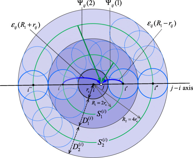
Schematic figure for representing the interactions used in the IPS method under the isotropic boundary condition. The center circle is the “local region” of atom i, a sphere with radius r_c, containing other atoms j, etc. $D_1^{(i)}$ [$D_2^{(i)}$] is a spherical shell (which is the annulus in this 2D representation) with a small radius r_c [3r_c] and a large radius 3r_c [5r_c]. $S_1^{(i)}$ [$S_2^{(i)}$] is a circle with a radius 2r_c [4r_c] and contained in $D_1^{(i)}$ [$D_2^{(i)}$]. Shown is only for m = 1,2. Dotted circles represent copies of the local region (called “image regions”), while, for calculating the interactions, the continuum approximation $S_1^{(i)},S_2^{(i)},\cdots$ are actually used instead, which can be viewed as continued images of $i^{\prime },i^{\prime \prime },\cdots ,$ respectively (see Appendix C (ii)). The “spherical interaction” (or “random interaction”) is interactions to atom j from spheres $S_1^{(i)},S_2^{(i)},\cdots$ (see Eq. 93). The “axial interaction” (Appendix C (iii)) is interactions to atom j from atoms $i^{\prime },i^{\circ },i^{\prime \prime },i^{\circ \circ },\cdots ,$ which are i’s copy along the j − i axis, ε_ij(R₁ − r_ij) + ε_ij(R₁ + r_ij) + ⋯ (see Eq. 94)

$$E_{ij}^{\text{IPS}}(r_{ij})={\epsilon }_{ij}(r_{ij})+\sum _{m\in \mathbb{\mathbb{N}}}{\tilde{\epsilon }}_{ij}(r_{ij};m)\text{for}j\in {\mathcal{N}}_i,$$ 13a

$$E_i^{\text{IPS}}(x)=\sum _{j\in {\mathcal{R}}_i}{E}_{ij}^{\text{IPS}}(r_{ij})+\sum _{m\in \mathbb{\mathbb{N}}}{\tilde{\epsilon }}_{ii}(r_{ii};m)$$ 13b

$$=\sum _{j\in {\mathcal{R}}_i}{\epsilon }_{ij}(r_{ij})+\sum _{j\in {\mathcal{R}}^i}\sum _{m\in \mathbb{\mathbb{N}}}{\tilde{\epsilon }}_{ij}(r_{ij};m)\mathrm{.}$$ 13c

Here, we restrict our discussion in the case of

$${\epsilon }_{ij}(r)=q_i{q}_j/r,$$ 14

but the IPS method can be formulated for other interactions; ${\mathcal{R}}^i$ and ${\mathcal{R}}_i$ are given in Eqs. 3 and 4, respectively. Note that there is a case that a factor 1/2 is attached for Eqs. 13b and 13c (e.g., Wu and Brooks 2005, 2019) for formulating theories, while not attached (Ojeda-May and Pu 2014a) for calculating Madelung energies, wherein we follow the latter definition, which is also parallel to Eqs. 12b and 12c in the PBC. The index $m\in \mathbb{\mathbb{N}}$ labels the radial direction centered at r_i, with letting R_m = 2mr_c, which captures the radius of concentric spheres. The image regions are placed inside each m-indexed spherical shell

$$D_m^{(i)}\equiv \{\mathbf{r}\in {\mathbb{ℝ}}^3|R_m-r_{\mathrm{c}}\le ∥\mathbf{r}-{\mathbf{r}}_i∥<R_m+r_{\mathrm{c}}\}\mathrm{.}$$ 15

These shells decompose the total space such that ${\mathbb{ℝ}}^3={\bigsqcup }_{m\in \mathbb{\mathbb{N}}}{D}_m^{(i)}\bigsqcup D_0^{(i)}$, where $D_0^{(i)}$ be the local region. On the other hand, the spherical directions are captured as an integration of continuously distributed individual copy. ${\tilde{\epsilon }}_{ij}$ includes all the effects such as this integration, as described below and detailed in Appendix C. ${\sum }_{m\in \mathbb{\mathbb{N}}}{\tilde{\epsilon }}_{ii}(r_{ii};m)$ in the second term of Eq. 13b represents self interaction.

The common feature between Eqs. 12 and 13 is clear, as interpreted by the correspondence:

$$\begin{array}{ccc}\mathcal{N}& \iff & {\mathcal{R}}^i\\ \text{(}{\mathcal{N}}_i& \iff & {\mathcal{R}}_i\text{)}\\ {\sum }_{n\in {\mathbb{\mathbb{Z}}}^3-\{0\}}{\epsilon }_{ij}(r_{ijn})& \iff & {\sum }_{m\in \mathbb{\mathbb{N}}}{\tilde{\epsilon }}_{ij}(r_{ij};m)\end{array}$$ 16

Namely, (i) the all atoms in the basic cell,$\mathcal{N}$, in the PBC corresponds to all the atoms in the local region,${\mathcal{R}}^i$ in the IBC. Accordingly, ${\mathcal{N}}_i$ corresponds to ${\mathcal{R}}_i$; (ii) while the interaction energy between atom j in the basic cell and all the copies of atom i in the PBC is ${\sum }_{n\in {\mathbb{\mathbb{Z}}}^3-\{0\}}{\epsilon }_{ij}(r_{ijn})$, it corresponds to the interaction energy between atom j in the local region and all the copies of atom i in the IBC, ${\sum }_{m\in \mathbb{\mathbb{N}}}{\tilde{\epsilon }}_{ij}(r_{ij};m)$; (iii) the self interaction in the PBC, which is obtained by replacing $ij\to ii$ in the left side of the third equation in (16), corresponds to the self interaction in the IBC, which is obtained by replacing $ij\to ii$ in the right side of the last equation in Eq. 16.

On the other hand, the difference between Eqs. 12 and 13 is seen in: (1) For the PBC, the fundamental region (basic cell) and the atoms ($\mathcal{N}$) are common for all i, but for the IBC, the fundamental region (local region) and the atoms (${\mathcal{R}}^i$) depend on each i; (2) the IBC assumes the special dependence of the energy, ${\tilde{\epsilon }}_{ij}(r_{ij};m)$, which is on a separated contribution from distance r_ij and index m.

As discussed in Appendix C, ${\tilde{\epsilon }}_{ij}$ is defined through several procedures, and we have

$${\mathrm{\Phi }}_{ij}^{\text{IPS}}(r)\equiv \sum _{m\in \mathbb{\mathbb{N}}}{\tilde{\epsilon }}_{ij}(r;m)$$ 17a

$$=-\frac{q_i{q}_j}{2r_{\mathrm{c}}}\left[\psi \left(1-\frac{r}{2r_{\mathrm{c}}}\right)\right)$$

$$\left(+\psi \left(1+\frac{r}{2r_{\mathrm{c}}}\right)+2\gamma \right],$$ 17b

where ψ is the digamma function, and γ is the Euler-Mascheroni constant. Using the notation

$$\begin{array}{rcl}{E}_{ij}^{\text{IPS}}(r_{ij})& \equiv & q_i{q}_j{\widehat{E}}^{\text{IPS}}(r_{ij})\\ & =& {\epsilon }_{ij}(r_{ij})+{\mathrm{\Phi }}_{ij}^{\text{IPS}}(r_{ij}),\end{array}$$ 18

we have the total energy of the IPS method (see Appendix C),

$$\begin{array}{rcl}{E}^{\text{IPS}}(x)& =& \frac{1}{2}\sum _{i\in \mathcal{N}}\sum _{j\in {\mathcal{R}}_i}{q}_i{q}_j\left[{\widehat{E}}^{\text{IPS}}(r_{ij})-{\widehat{E}}^{\text{IPS}}(r_{\mathrm{c}})\right]\\ & -& \frac{{\widehat{E}}^{\text{IPS}}(r_{\mathrm{c}})}{2}\sum _{i\in \mathcal{N}}{q}_i^2+\frac{{\widehat{E}}^{\text{IPS}}(r_{\mathrm{c}})}{2}\sum _{i\in \mathcal{N}}{q}_i\sum _{j\in {\mathcal{R}}^i}{q}_j\mathrm{.}\end{array}$$ 19

Here the right first term is a pairwise summation form with a cutoff procedure and the second term is called the self-energy term. The last term is called the “boundary energy,” whose approximation method is discussed in Appendix C (vi).

Note that, for ease in the computational handling, several approximations of

$${\mathrm{\Phi }}_{ij}^{\text{IPS}}(r)\equiv q_i{q}_j{\widehat{\mathrm{\Phi }}}^{\text{IPS}}(r)$$ 20

have been proposed to avoid the use of ψ (Wu and Brooks 2005, 2008), such as ${\widehat{\mathrm{\Phi }}}^{\text{IPS}}(r)$ being a polynomial (Wu and Brooks 2008).

IPSp method

The method introduced in “Isotropic periodicity principle” is derived based on a nonpolar homogeneous approximation, so that it is labelled as IPSn method. The IPSp method derives a polar electrostatic 3D-IPS potential (Wu and Brooks 2009). The pair potential function in the IPSp method is defined by adding a certain “screening” function ${\mathrm{\Phi }}_{ij}^{\text{Screen}}(r_{ij})$ into the original IPSn pair potential function (18). In other word, the IPSp method is obtained by replacing ${\mathrm{\Phi }}_{ij}^{\text{IPS}}(r_{ij})$ into

$${\mathrm{\Phi }}_{ij}^{\text{IPSp}}(r_{ij}):={\mathrm{\Phi }}_{ij}^{\text{IPS}}(r_{ij})+{\mathrm{\Phi }}_{ij}^{\text{Screen}}(r_{ij}),$$ 21

and we have

$$E_{ij}^{\text{IPSp}}(r_{ij})={\epsilon }_{ij}(r_{ij})+{\mathrm{\Phi }}_{ij}^{\text{IPSp}}(r_{ij}),$$ 22

instead of $E_{ij}^{\text{IPS}}(r_{ij})$ (see Eqs. 13a and 18). In the IPSp method, ${\mathrm{\Phi }}_{ij}^{\text{Screen}}$ is defined by ${\mathrm{\Phi }}_{ij}^{\text{Screen}}(r)=q_i{q}_j{\widehat{\mathrm{\Phi }}}^{\text{Screen}}(r)$ with using a polynomial

$${\widehat{\mathrm{\Phi }}}^{\text{Screen}}(r)\equiv \sum _{m=1}^L{b}_m{r}^{2m},$$ 23

and the coefficients b_ms are determined by constraints:

$$D^m{\widehat{E}}^{\text{IPSp}}(r_{\mathrm{c}})=0\text{for}m=1,\dots ,L\mathrm{.}$$ 24

Here we have denoted as $E_{ij}^{\text{IPSp}}(r)\equiv q_i{q}_j{\widehat{E}}^{\text{IPSp}}(r)$ (cf. (18)).

A physical interpretation for Eqs. 21 and 24 is not so straightforward. Original work is based on considering that ${\widehat{\mathrm{\Phi }}}^{\text{Screen}}(r)$ represents a screening effect by opposite-charge distribution around each charge in polar systems and that there are interactions with dipoles, which yield charge-dipole interactions, resulting in m = 2 condition in Eq. 24, and dipole-dipole interactions (m = 3), as well as charge-charge interactions (m = 1).

Three remarks are made. (1) Note that ${\widehat{\mathrm{\Phi }}}^{\text{Screen}}$ is specific to electrostatic interactions, whereas ${\mathrm{\Phi }}_{ij}^{\text{IPS}}$ can be constructed within the same procedure for any interactions such as the LJ type, instead of the electrostatic interaction. (2) It should be stressed that ${\widehat{\mathrm{\Phi }}}^{\text{Screen}}(r)$ is treated to work only as the axial interactions (see Appendix C (iii)), not as the spherical interactions. This is a characteristic choice, because a non-Coulombic function could contribute to spherical interactions (while pure Coulombic interactions cannot contribute to spherical interactions, as stated in Appendix C (v)). From this choice, a symmetry with respect to the line i − j arises, and the force between j and all “i”s in the line becomes zero when j is at the local region boundary (i.e., r_ij = r_c). (3) Another conceivable idea based on a physical viewpoint regarding Eq. 24 is that the screening effect can be measured not only for a charge that is really placed at the site j but also for a multipole that is imaginary placed at the site j. Considering that the charge–charge interaction is described by E^IPSp(r), an interaction potential and a force between a charge q_i and an m th-moment multipole (m = 0,…,L − 1) are proportional to $D^m{\widehat{E}}^{\text{IPSp}}(r)$ and $D^{m+1}{\widehat{E}}^{\text{IPSp}}(r)$, respectively. Here we have assumed that the multipoles have nonvanishing components only for the i − j direction (line multipole). This idea contributes to a possible supplementary explanation to justify Eq. 24.

The energy functions for the IPSp method are obtained by the replacement of ${\mathrm{\Phi }}_{ij}^{\text{IPS}}$ into ${\mathrm{\Phi }}_{ij}^{\text{IPSp}}$. Thus, in the IPSp method, $E_i^{\text{IPS}}(x)$ (see Eq. 13b) is replaced into

$$\begin{array}{rcl}{E}_i^{\text{IPSp}}(x)& =& \sum _{j\in {\mathcal{R}}_i}{E}_{ij}^{\text{IPSp}}(r_{ij})+{\mathrm{\Phi }}_{ii}^{\text{IPSp}}(r_{ii})\\ & =& \sum _{j\in {\mathcal{R}}_i}{E}_{ij}^{\text{IPSp}}(r_{ij}),\end{array}$$ 25

where we have used ${\mathrm{\Phi }}_{ii}^{\text{IPS}}(0)={\mathrm{\Phi }}_{ii}^{\text{Screen}}(0)=0$, and E^IPS (see Eq. 19) is replaced into

$$\begin{array}{rcl}{E}^{\text{IPSp}}(x)& =& \frac{1}{2}\sum _{i\in \mathcal{N}}\sum _{j\in {\mathcal{R}}_i}{q}_i{q}_j\left[{\widehat{E}}^{\text{IPSp}}(r_{ij})-{\widehat{E}}^{\text{IPSp}}(r_{\mathrm{c}})\right]\\ & -& \frac{{\widehat{E}}^{\text{IPSp}}(r_{\mathrm{c}})}{2}\sum _{i\in \mathcal{N}}{q}_i^2+\frac{{\widehat{E}}^{\text{IPSp}}(r_{\mathrm{c}})}{2}\sum _{i\in \mathcal{N}}{q}_i\sum _{j\in {\mathcal{R}}^i}{q}_j\mathrm{.}\\ & & \end{array}$$ 26

Neutralization principle

Each of the RF, IPS, and LS methods is an “addition method” that tries to incorporate the effects beyond the truncation region (which corresponds to the cavity, local region, and basic cell, respectively), whereas the ZMM discussed in this subsection is a “subtraction method” that tries to remove artificial effects from the truncation region (which corresponds to a cutoff sphere), where the artificial effects are generated near the boundary of the cutoff sphere.

As discussed in “Introduction,” we do not need to consider interactions from so far away that the rate of the information transfer exceeds the speed of light. In the most simple cutoff, i.e., the straight truncation, each charge i feels the interactions from every charge j only in the cutoff sphere with the radius of a given cutoff length r_c:

$$\frac{1}{2}\sum _{i\in \mathcal{N}}\sum _{j\in {\mathcal{R}}_i}\frac{q_i{q}_j}{r_{ij}}\mathrm{.}$$ 27

Then, is a cutoff length of 10 Å too short? Given that the potential function value decays with the distance between atoms, is it more accurate to increase the cutoff length even a little? In fact, it has been shown that this is not the case; Yonetani (2006) shows that the longer the r_c, the worse the results can be. What, then, is the essential problem with the CB method?

The reason is that the usual CB method takes in just all interactions within the cutoff length, which is pure distance clipping of interactions. A specific problem is that high-energy states, e.g., configurations gathering only positive charges, may occur just inside the cutoff region, which is artificially prepared. Although no such high-energy states can be directly observed with a slight change in the region surrounding such a state, such states are virtually present when applying the straight truncation (Fig. 4). High-energy configurations (or also extremely low-energy configurations) should be excluded, considering the canonical distribution at the room temperature, the most encountered situation in equilibrium molecular simulation. However, because the straight truncation incorporates the interactions from such a state, this can give false information to the central atom i. Moreover, immediate decay of such a state, as expected in a sufficiently wide region under the canonical distribution if it were generated, does not necessarily occur inside the clipping region.

Fig. 4.

Schematic figure for representing a neutralized subset ${\mathcal{M}}_i^{(l)}$ (composed from atoms in the green shaded region) in the cutoff sphere ${\mathcal{R}}_i$ with a radius r_c around atom i having charge + 1 denoted by “ + ” (while “−” denotes an atom with charge − 1). Excess subset ${\mathcal{J}}_i^{(l)}$ contains 5 positive charges, where, in particular, the 3 bold font “+ ” charges in the left side seem to provide a high energy state in the cutoff sphere

The basic policy of ZMM (Fukuda et al. 2011; Fukuda 2013) corresponds to discarding the virtual high-energy states arising just inside the artificial cutoff boundary. In other words, it is a method of “subtraction,” i.e., not counting interactions from such states, and discarding them. Since these virtual high energy states derive from the violation of the local electrostatic neutrality, ZMM takes into account electrostatically neutralized configurations inside the cutoff sphere. The neutrality is considered locally and is acceptable even if it is approximately attained. In addition, the neutralization should not only be for the charges but also dipole and higher multipole if needed.

That is, (nearly) neutralized configuration, which is called a neutralized subset, is utilized in the ZMM (Fukuda et al. 2011; Fukuda 2013):

$$\frac{1}{2}\sum _{i\in \mathcal{N}}\sum _{j\in {\mathcal{M}}_i^{(l)}}\frac{q_i{q}_j}{r_{ij}},$$ 28

where ${\mathcal{M}}_i^{(l)}$ is the neutralized subset in the sense of l th-(multi)pole with respect to charge i (see Fig. 4). However, seeking the neutralized subset HCode ${\mathcal{M}}_i^{(l)}$ may be time consuming in practice. Thus, the calculation of ${\mathcal{M}}_i^{(l)}$ is not required, but instead, just its existence is assumed. Our strategy is that we return to a simple cutoff sum form but instead deform the Coulomb pair potential function into a certain function ${\mathcal{U}}^{(l)}$ in order to approximate the neutralized sum (28) such that

$$\frac{1}{2}\sum _{i\in \mathcal{N}}\sum _{j\in {\mathcal{M}}_i^{(l)}}\frac{q_i{q}_j}{r_{ij}}\simeq \frac{1}{2}\sum _{i\in \mathcal{N}}\sum _{j\in {\mathcal{R}}_i}{q}_i{q}_j{\mathcal{U}}^{(l)}(r_{ij})+\text{const}\mathrm{.}$$ 29

To justify this idea and specifically formulate ${\mathcal{U}}^{(l)}$, it relies on the following three conditions for characterizing ${\mathcal{M}}_i^{(l)}$:

$$\forall j\in {\mathcal{M}}_i^{(l)},r_{ij}<r_{\mathrm{c}},$$ 30a

$$\sum _{j\in {\mathcal{M}}_i^{(l)}\cup \{i\}}{q}_j{\mathbf{r}}_j\otimes \stackrel{m}{\dots }\otimes {\mathbf{r}}_j=0\text{for}m=0,\dots ,l,$$ 30b

$$\forall j\in {\mathcal{N}}_i-{\mathcal{M}}_i^{(l)},(r_{ij}<r_{\mathrm{c}}\Rightarrow r_{ij}\simeq r_{\mathrm{c}})\mathrm{.}$$ 30c

The first two conditions are just the ones explained above. The last one indicates that the charges (≠i) excluded from the neutralized subset ${\mathcal{M}}_i^{(l)}$ in the cutoff sphere of i are located close to the cutoff surface. In other words, the neutrality is broken near the cutoff surface that is the boundary of the ad hoc chosen perfect sphere shape (which by itself does not necessarily ensure the neutrality). Using these three conditions along with a consistency condition (which is just the action-reaction condition), Eq. 29 can be mathematically deduced (Fukuda 2013).

To briefly review it, we first fix some notations: $\widehat{\epsilon }(r)=1/r$ is the Coulombic kernel, and

$${\mathcal{J}}_i^{(l)}\equiv {\mathcal{R}}_i-{\mathcal{M}}_i^{(l)}$$ 31

is an excess subset, which is a subset of charges whose interactions to charge i should be subtracted. That is, the total energy E(x) is represented as

$$E(x)\simeq \frac{1}{2}\sum _{i\in \mathcal{N}}\sum _{j\in {\mathcal{M}}_i^{(l)}}{q}_i{q}_j\widehat{\epsilon }(r_{ij})$$ 32a

$$\begin{array}{rcl}& =& \frac{1}{2}\sum _{i\in \mathcal{N}}\sum _{j\in {\mathcal{R}}_i}{q}_i{q}_j\widehat{\epsilon }(r_{ij})-\frac{1}{2}\sum _{i\in \mathcal{N}}\sum _{j\in {\mathcal{J}}_i^{(l)}}{q}_i{q}_j\widehat{\epsilon }(r_{ij}),\\ & & \end{array}$$ 32b

wherein the second line means that interactions from the excess subset. $\frac{1}{2}{\sum }_{i\in \mathcal{N}}{\sum }_{j\in {\mathcal{J}}_i^{(l)}}{q}_i{q}_j\widehat{\epsilon }(r_{ij})$ which is called the excess energy, is subtracted from the interactions from all charges in the cutoff sphere, $\frac{1}{2}{\sum }_{i\in \mathcal{N}}{\sum }_{j\in {\mathcal{R}}_i}{q}_i{q}_j\widehat{\epsilon }(r_{ij})$. As reviewed in Appendix D, by using a suitable polynomial

$${\widehat{\epsilon }}_l(r)\equiv \sum _{m=0}^l{a}_m^{(l)}{r}^{2m},$$ 33

the excess energy can be approximated by a pairwise form for this polynomial, allowing the subtraction to be accomplished using a pairwise form,

$$E(x)\simeq \frac{1}{2}\sum _{i\in \mathcal{N}}\sum _{j\in {\mathcal{R}}_i}{q}_i{q}_j\left[\widehat{\epsilon }(r_{ij})-{\widehat{\epsilon }}_l(r_{ij})\right]-\frac{a_0^{(l)}}{2}\sum _{i\in \mathcal{N}}{q}_i^2\mathrm{.}$$ 34

This formula accords with the RHS of Eq. 29 with ${\mathcal{U}}^{(l)}(r)=\widehat{\epsilon }(r)-{\widehat{\epsilon }}_l(r)$.

The above procedure utilizes the bare (undamped) Coulombic function $\widehat{\epsilon }(r)=1/r$ in the starting point of Eq. 27. In general, the same procedure can be applied to a damped function V (r), by suitably treating the remaining part $\frac{1}{r}-V(r)$. Specifically, the energy function of the ZMM can be represented by

$$\begin{array}{rcl}{E}_{\text{ZM}}^{(l)}(x)& \equiv & \frac{1}{2}\sum _{i\in \mathcal{N}}\sum _{j\in {\mathcal{R}}_i}{q}_i{q}_j\left[V(r_{ij})-V_l(r_{ij})\right]\\ & -& \left(\frac{{\tilde{a}}_0^{(l)}}{2}+\frac{\alpha }{\sqrt{\pi }}\right)\sum _{i\in \mathcal{N}}{q}_i^2\mathrm{.}\end{array}$$ 35

Here, in the first term,

$$V(r)\equiv \frac{\text{erfc}(\alpha r)}{r}$$ 36

is the damped Coulombic function, and the remaining function $\frac{1}{r}-V(r)$ contributes the last term of Eq. 35, viz., $-\frac{\alpha }{\sqrt{\pi }}{\sum }_{i\in \mathcal{N}}{q}_i^2$. In the pairwise term,

$$V_l(r)\equiv \sum _{m=0}^l{\tilde{a}}_m^{(l)}{r}_{ij}^{2m}$$ 37

is the polynomial whose degree depends on the multipole moment l, and the coefficients ${\tilde{a}}_m^{(l)}$ are uniquely determined and depend on α, l, and r_c (Fukuda 2013). Note that α = 0 reduces $E_{\text{ZM}}^{(l)}(x)$ into the RHS of Eq. 34 , and in particular

$${\tilde{a}}_m^{(l)}{|}_{\alpha =0}=a_m^{(l)}$$ 38

for all l and m.

The argument that “subtraction methods have artifacts and addition methods do not” is incorrect. The first reason is that these criticisms are based on the results of older literature (e.g., Koehl 2006; Izvekov et al. 2008) which mostly refer to artifacts in the straight truncation or group-based cutoff (Baumketner 2009) and do not refer to the artifact of the CB method in general, nor to the artifact of the subtraction method in the CB method. In fact, for example, ZMM, a subtraction CB method, shows that there is no unignorable artifact in polar fluids such as water systems (Fukuda et al. 2014; Wang et al. 2016b), DNA in explicit solvent as a highly charged system (Arakawa et al. 2013), and a ferroelectric crystal as a dipolar system (Wang et al. 2016b). Rather, the method also helped to clarify the artifact in the PBC (Kasahara et al. 2018b). The second reason is rather conspicuous, that is, the subtraction method, ZMM, can be equal to an addition method, IPS method, as will be shown in the next section. Finally, it is also noted that the subtraction method idea allows us to obtain the continuity for energy functions (see Appendix A), but there is no known case where this can be achieved by use of an addition method idea.

Other methods

One of other promising electrostatic interaction calculation methods is the fast multipole method (Greengard and Rokhlin 1987), which uses the multipole expansion in a suitably divided cell, utilizing the feature that the pair potential function decays as the atomic length is larger. Its recent development is provided in literature (Poursina and Anderson 2014; Alouges and Aussal 2015; March and Biros 2017; Abeyratne et al. 2019; Urano et al. 2020).

A quantitatively different approach for calculating electrostatic interactions is to utilize non-Euclidean geometry, such as 3-dimensional sphere S³ (Caillol 1999; Ramírez EV and Elvingson 2022), instead of ${\mathbb{ℝ}}^3$. Recently, Clifford torus is also considered and applied to calculate Madelung energy of crystal systems (Tavernier et al. 2021).

Relationships among non-Ewald methods

Mathematically unified form

There is a common mathematical structure in the form of the energy function among the non-Ewald method stated in the previous sections. As stated in literature (Fukuda and Nakamura 2012; Fukuda 2013), the energy function follows the form:

$$\begin{array}{rcl}E(x)& =& \frac{1}{2}\sum _{i\in \mathcal{N}}\sum _{j\in {\mathcal{R}}_i}{q}_i{q}_j\left[u(r_{ij})-u(r_{\mathrm{c}})\right]\\ & & -\frac{1}{2}\left[u(r_{\mathrm{c}})+\frac{2\alpha }{\sqrt{\pi }}\right]\sum _{i\in \mathcal{N}}{q}_i^2\mathrm{.}\end{array}$$ 39

Here, the first term is the pairwise sum using a basic function u that defines a pair potential function

$$r\mapsto \left\{\begin{array}{cc}u(r)-u(r_{\mathrm{c}})& \text{for}0<r<r_{\mathrm{c}}\\ 0& \text{for}r\ge r_{\mathrm{c}}\end{array}\right\},$$ 40

which is at least continuous. The second term $-\frac{1}{2}u(r_{\mathrm{c}}){\sum }_{i\in \mathcal{N}}{q}_i^2$ is the self-energy term, which can be viewed as the i = j term arising inside the first term. The last term comes from the choice of the kernel as the Ewald real function (see Eq. 36) and works as a correction of the energy on this choice.

CB methods taking this form are summarized in Fig. 5, and the relationships among these methods will be discussed in the following subsections.

Fig. 5.

Relationships among non-Ewald methods: Pre-averaging (PA) (Yakub and Ronchi 2003); FSw-Wolf (Fukuda et al. 2008); Wolf (Wolf et al. 1999); Harrison (Harrison 2006); modified reaction field (MRF) (Barker and Watts 1973; Fukuda and Nakamura 2012); generalized reaction field (GRF) (Hummer et al. 1994); modified IPSp (MIPSp) (Wu and Brooks 2009; and see Eq. 59); IPSn (Wu and Brooks 2005); zero multipole summation method (ZMM) (Fukuda 2013); non-damped ZMM (Nd-ZMM); and non-damped zero-dipole (Nd-ZD) (Fukuda et al. 2011). A dashed line shows an approximate relationship

Relationship between the RF method and the ZMM

The energy function of the ZMM can be rewritten (see Appendix D) as

$$\begin{array}{rcl}{E}_{\text{ZM}}^{(l)}(x)& =& \frac{1}{2}\sum _{i\in \mathcal{N}}\sum _{j\in {\mathcal{R}}_i}{q}_i{q}_j\left[u^{(l)}(r_{ij})-u^{(l)}(r_{\mathrm{c}})\right]\\ & -& \frac{1}{2}\left[u^{(l)}(r_{\mathrm{c}})+\frac{2\alpha }{\sqrt{\pi }}\right]\sum _{i\in \mathcal{N}}{q}_i^2,\end{array}$$ 41

where u^(l) is the basic function represented by

$$u^{(l)}(r)\equiv V(r)-\sum _{m=1}^l{\tilde{a}}_m^{(l)}{r}^{2m}\mathrm{.}$$ 42

Thus, it exactly takes the form of Eq. 39 with u ≡ u^(l). The ZMM with l = 1 and l = 0 are the zero dipole (ZD) method (Fukuda et al. 2011; 2012) and the Wolf method (Wolf 1992; Wolf et al. 1999), respectively. The ZMM with l = 0 and α = 0 is also considered to be the same as the scheme by Harrison (2006) (see Fukuda (2013)). ZMM with α = 0 is indicated as non-damped ZMM (Nd-ZMM) in Fig. 5. The force-switching (FSw) Wolf method (Fukuda et al. 2008) is the scheme modifying the Wolf method to use it in MD with a smooth force function using a switching length r₁.

The energy of the modified RF (MRF), Eq. 11, also takes the form of Eq. 39 with u ≡ V_RF and α = 0. As pointed out before (Fukuda and Nakamura 2012; Fukuda 2013), we can see the basic function correspondence between V_RF of the RF and u⁽¹⁾ of the ZMM (ZD), ${\left(V_{\text{RF}}\right|}_{{𝜖}_{\text{RF}}\to \infty }={\left(u^{(1)}\right|}_{\alpha =0}$. Note that an interpretation of the ZD method relating to the RF principle is discussed by Elvira and MacDowell (2014), where the dipole in the medium causes an electric field, which defines the force and its integration leads to the a potential function u⁽¹⁾(r_ij) − u⁽¹⁾(r_c).

Relationship between the IPSp method and the ZMM

We show an equivalence between the pair potential function of the IPSp method with a polynomial approximation and the pair potential function of the ZMM with α = 0 and l = 3. As shown in Appendix D, the pair function of the ZMM, u^(l) for l = 3, is given by

$$u^{(3)}{|}_{\alpha =0}(r)=\frac{1}{r}+\frac{35}{16}\frac{r^2}{r_{\mathrm{c}}^3}-\frac{21}{16}\frac{r^4}{r_{\mathrm{c}}^5}+\frac{5}{16}\frac{r^6}{r_{\mathrm{c}}^7}\mathrm{.}$$ 43

While in the IPSp method (Wu and Brooks 2009), the following approximated function, ${\widetilde{\widehat{\mathrm{\Phi }}}}^{\text{IPS}}(r)$, is used instead of ${\widehat{\mathrm{\Phi }}}^{\text{IPS}}(r)$: (i) it is a polynomial in the form of

$${\widetilde{\widehat{\mathrm{\Phi }}}}^{\text{IPS}}(r)\equiv \sum _{m=1}^M{c}_m{r}^{2m},$$ 44

as well as ${\widehat{\mathrm{\Phi }}}^{\text{Screen}}(r)$ (see Eq. 23); (ii) M = 3 is chosen (see Eq. 8 in Wu and Brooks (2009)). Corresponding to this polynomial approximation, replace ${\widehat{E}}^{\text{IPSp}}(r)$ by

$${\tilde{\widehat{E}}}^{\text{IPSp}}(r)\equiv \widehat{\epsilon }(r)+{\widetilde{\widehat{\mathrm{\Phi }}}}^{\text{IPS}}(r)+{\widehat{\mathrm{\Phi }}}^{\text{Screen}}(r)$$ 45

and (iii) choose L = 3 for ${\widehat{\mathrm{\Phi }}}^{\text{Screen}}(r)$. These strategies result in (see Eq. 15 in Wu and Brooks (2009))

$${\tilde{\widehat{E}}}^{\text{IPSp}}(r)=\frac{1}{r}\left[1+\frac{35}{16}\frac{r^3}{r_{\mathrm{c}}^3}-\frac{21}{16}\frac{r^5}{r_{\mathrm{c}}^5}+\frac{5}{16}\frac{r^7}{r_{\mathrm{c}}^7}\right]\mathrm{.}$$ 46

Comparing Eqs. 43 and 46, we see the equality of the basic functions between the ZMM with l = 3, α = 0 and the IPSp method, i.e.,

$$u^{(3)}{|}_{\alpha =0}(r)={\tilde{\widehat{E}}}^{\text{IPSp}}(r)$$ 47

for all r, and we also observe the equality of the pair potential functions of both methods (see the first term of RHS of Eq. 26; see also Eq. 19 in Wu and Brooks (2009)):

$$u^{(3)}{|}_{\alpha =0}(r)-u^{(3)}{|}_{\alpha =0}(r_{\mathrm{c}})={\tilde{\widehat{E}}}^{\text{IPSp}}(r)-{\tilde{\widehat{E}}}^{\text{IPSp}}(r_{\mathrm{c}})$$ 48a

$$=:{\widehat{\widehat{E}}}^{\text{IPSp}}(r)\mathrm{.}$$ 48b

Now we consider the reason of the correspondence, (47). In the ZMM with α = 0, to obtain the l th-order approximation of the excess energy, we require the following condition (see Eq. 33 and Appendix D):

$$D^m\widehat{\epsilon }(r_{\mathrm{c}})=D^m{\widehat{\epsilon }}_l(r_{\mathrm{c}})\text{for}m=0,\dots ,l\mathrm{.}$$ 49

Equation 49 with l = 3 is represented as

$${\left(\frac{d^m}{d{r}^m}\left[\frac{1}{r}-\sum _{m=0}^3{a}_m^{(3)}{r}^{2m}\right]\right|}_{r=r_{\mathrm{c}}}=0\text{for}m=0,\dots ,3.$$ 50

This is an invertible linear equation with respect to ${\{a_m^{(3)}\}}_{m=0,1,\dots ,3}$, and thus uniquely solved (Fukuda 2013). While for the IPSp, the method to determine polynomial coefficients via Eq. 24 is rewritten by the strategies (i)–(iii) such that

$$D^m{\widehat{\widehat{E}}}^{\text{IPSp}}(r_{\mathrm{c}})=0\text{for}m=0,\dots ,3,$$ 51

with

$${\widehat{\widehat{E}}}^{\text{IPSp}}(r)=\frac{1}{r}+\sum _{m=0}^3{d}_m{r}^{2m},$$ 52

where we have put

$$d_m\equiv c_m+b_m\text{for}m\ge 1$$ 53

and defined d₀ by

$$d_0\equiv -{\tilde{\widehat{E}}}^{\text{IPSp}}(r_{\mathrm{c}})=-\left[\widehat{\epsilon }(r_{\mathrm{c}})+{\widetilde{\widehat{\mathrm{\Phi }}}}^{\text{IPS}}(r_{\mathrm{c}})+{\widehat{\mathrm{\Phi }}}^{\text{Screen}}(r_{\mathrm{c}})\right]$$ 54

to meet Eq. 51 for m = 0. Since c_m are given quantities, solving Eq. 51 with respect to {b_m}_{m= 0,1,…,3} is equivalent to solve

$$0={\left(\frac{d^m}{d{r}^m}\left[\frac{1}{r}+\sum _{m=0}^3{d}_m{r}^{2m}\right]\right|}_{r=r_{\mathrm{c}}}\text{for}m=0,\dots ,3.$$ 55

with respect to {d_m}_{m= 0,1,…,3}. Since Eq. 55 has the same form as Eq. 50, ${\{d_m^{(l)}\}}_{m=0,1,\dots ,3}$ is uniquely obtained to be

$$d_m=-a_m^{(3)}\text{for}m=0,\dots ,3.$$ 56

Considering the fact that the pair potential function of the ZMM is $u^{(3)}{|}_{\alpha =0}(r)-u^{(3)}{|}_{\alpha =0}(r_{\mathrm{c}})=\widehat{\epsilon }(r)-{\widehat{\epsilon }}_l(r)=\frac{1}{r}-{\sum }_{m=0}^3{a}_m^{(3)}{r}^{2m}$ (see Eqs. 37 and 38 and Appendix D, Eq. (116)) and that of the IPSp method is given by Eq. 52, they are the same owing to Eq. 56 . Thus, we have obtained the proof of Eq. 48a. Equation 47 follows from this and from the fact that ${\tilde{\widehat{E}}}^{\text{IPSp}}(r_{\mathrm{c}})=u^{(3)}{|}_{\alpha =0}(r_{\mathrm{c}})$, which is derived from Eqs. 54 , 56, 38, and 115.

To summarize, between the IPSp and the ZMM with α = 0 and l = 3, the equations determining the polynomials that define the common pair potential function form are mathematically the same. Recall that, however, the physical motivations for the polynomial determination are different between the two methods: the ZMM with α = 0 and l = 3 motivates to have the third order approximation of the excess energy error, while the IPSp motivates to realize the IBC and adapt to polar systems. It should be noted that the equivalence, (47), is owing to strategies (i)–(iii) stated above. If we do not choose these strategies, the exact equivalence is not expected to be obtained. In fact, (i) is not chosen by Wu and Brooks (2005), for which ${\widehat{\mathrm{\Phi }}}^{\text{IPS}}(r)$ is not approximated as a pure polynomial (see Eq. 58 of Wu and Brooks (2005), which will also be shown in below Eq. 61, for the approximated form of $\widehat{\epsilon }(r)+{\widehat{\mathrm{\Phi }}}^{\text{IPS}}(r)$, and see also Eq. 38 of the literature for other potentials) (ii) is not chosen in (Wu and Brooks 2008), for which M = 6 is chosen (see Eq. 12 in Wu and Brooks (2008)). In general, to improve the accuracy of the approximation to the original pair function in numerical fitting, it will generally be advantageous to increase the number of coefficients involved in the approximate function (e.g., by increasing a polynomial degree, L or M). In fact, in IPSn, the deviation from the original function is measured by RMSD (Wu and Brooks 2005). In the IPSp, in contrast, the degrees of freedom of the fitting is lost by ignoring the higher order terms of the polynomial.

Regarding the energy function of the ZMM with α = 0 and l = 3 (see Eq. 41),

$$\begin{array}{rcl}{E}_{\text{ZM}}^{(3)}{|}_{\alpha =0}(x)& =& \frac{1}{2}\sum _{i\in \mathcal{N}}\sum _{j\in {\mathcal{R}}_i}{q}_i{q}_j\left[u^{(3)}{|}_{\alpha =0}(r_{ij})-u^{(3)}{|}_{\alpha =0}(r_{\mathrm{c}})\right]\\ & & -\frac{1}{2}{u}^{(3)}{|}_{\alpha =0}(r_{\mathrm{c}})\sum _{i\in \mathcal{N}}{q}_i^2,\end{array}$$ 57

and the approximate energy function of the IPSp (cf. (26)) is

$$\begin{array}{rcl}{E}^{\text{IPSp}}(x)& =& \frac{1}{2}\sum _{i\in \mathcal{N}}\sum _{j\in {\mathcal{R}}_i}{q}_i{q}_j\left[{\tilde{\widehat{E}}}^{\text{IPSp}}(r_{ij})-{\tilde{\widehat{E}}}^{\text{IPSp}}(r_{\mathrm{c}})\right]\\ & & -\frac{{\tilde{\widehat{E}}}^{\text{IPSp}}(r_{\mathrm{c}})}{2}\sum _{i\in \mathcal{N}}{q}_i^2+\frac{{\tilde{\widehat{E}}}^{\text{IPSp}}(r_{\mathrm{c}})}{2}\sum _{i\in \mathcal{N}}{q}_i\sum _{j\in {\mathcal{R}}^i}{q}_j\mathrm{.}\\ & & \end{array}$$ 58

Their pairwise summation terms and the self terms are the same as seen above. The difference between these two energy formulas is in the last term of Eq. 58, but these two will be the same if we use an approximation of subtracting the boundary term or adopting the charge neutrality, as detailed in Appendix C, noting that ${\tilde{\widehat{E}}}^{\text{IPSp}}(r_{\mathrm{c}})=35/16r_{\mathrm{c}}\ne 0$ owing to Eq. 46. Namely, if we denote an energy of a modified IPSp method by E^MIPSp(x)that is defined, using the above approximation, by

$$\begin{array}{rcl}{E}^{\text{MIPSp}}(x)& =& \frac{1}{2}\sum _{i\in \mathcal{N}}\sum _{j\in {\mathcal{R}}_i}{q}_i{q}_j\left[{\tilde{\widehat{E}}}^{\text{IPSp}}(r_{ij})-{\tilde{\widehat{E}}}^{\text{IPSp}}(r_{\mathrm{c}})\right]\\ & & -\frac{1}{2}{\tilde{\widehat{E}}}^{\text{IPSp}}(r_{\mathrm{c}})\sum _{i\in \mathcal{N}}{q}_i^2,\end{array}$$ 59

then it is the same as the ZMM energy with α = 0 and l = 3. It is reported in the study of a model liquid-crystal system (Nozawa et al. 2015b) that IPSn and IPSp methods indicate similar properties with that of the particle mesh Ewald method (Essmann et al. 1995) in a range of temperatures except for away from equilibria.

Other relationships

To compare pair potential functions in different methods, u − u(r_c), as employed in Eq. 39, it is often convenient to use, instead of $u:(0,r_{\mathrm{c}})\to \mathbb{ℝ}$ itself, a scaled function $v:(0,1)\to \mathbb{ℝ}$ characterized by

$$r_{\mathrm{c}}(u(r)-u(r_{\mathrm{c}}))=v(s)-v(1),$$ 60

where $s=\frac{r}{r_{\mathrm{c}}}$. This is because the original functions u often contain the parameter r_c so that r_c dependence should also be studied for their comparison, while functions v, which are scaled but completely capture the original functions u, are all parametrized by s ∈ (0,1) in a unit scale and may not contain r_c. In fact, the function v in the following methods, including the IPS, RF, and ZMM with α = 0, does not contain r_c.

1. IPSn is similar to the RF with low 𝜖_RF–.

   As indicated by Wu and Brooks (2005), the basic function of the IPS method, ${\widehat{E}}^{\text{IPS}}$, approximated such that

   $$\begin{array}{rcl}{\widehat{E}}^{\text{IPS}}(r)& \simeq & {\tilde{\widehat{E}}}^{\text{IPS}}(r)\equiv \frac{1}{r}+\frac{2.737821}{\sqrt{2}{r}_{\mathrm{c}}}\\ & & +\frac{1}{\sqrt{2r_{\mathrm{c}}^2-r^2}}\left(-2.737821+1.109466{\left(\frac{r}{r_{\mathrm{c}}}\right)}^2\right)\\ & & \left(+0.070800{\left(\frac{r}{r_{\mathrm{c}}}\right)}^4+0.007918{\left(\frac{r}{r_{\mathrm{c}}}\right)}^6\right)\end{array}$$ 61

   is similar to the basic function V_RF(r) in Eq. 10 with ${𝜖}_{\text{RF}}\sim 5$. The scaled function, characterized by Eq. 60, of the IPS ${\tilde{\widehat{E}}}^{\text{IPS}}$ is denoted as
   $$\begin{array}{rcl}& & {\tilde{\widehat{v}}}^{\text{IPS}}(s)=\frac{1}{s}+\frac{2.737821}{\sqrt{2}}+\frac{1}{\sqrt{2-s^2}}\\ & & \left(-2.737821+1.109466s^2+0.070800s^4+0.007918s^6\right),\end{array}$$ 62

   and the scaled function of the RF is

   $$v^{{}_{\text{RF}}}(s)=\frac{1}{s}+\frac{{𝜖}_{\text{RF}}-1}{2{𝜖}_{\text{RF}}+1}{s}^2,$$ 63

   where both scaled functions are independent of r_c. Figure 6 indicates ${\tilde{\widehat{v}}}^{\text{IPS}}-{\tilde{\widehat{v}}}^{\text{IPS}}(1)$ and $v^{{}_{\text{RF}}}-v^{{}_{\text{RF}}}(1)$ with 𝜖_RF = 5, as well as $v^{{}_{\text{RF}}}-v^{{}_{\text{RF}}}(1)$ with ${𝜖}_{\text{RF}}\to \infty$ for comparison.

2. GRF and ZMM with α = 0 and l = 4 are similar–.

   The generalized RF (GRF) method by Hummer et al. (1994) is derived from an attempt to eliminate the asymmetry in the RF method by assuming that the interacting distant atoms are also surrounded by a uniform background charge, and it has the following pair potential function:

   $$\begin{array}{rcl}{u}^{\text{GRF}}(r)-u^{\text{GRF}}(r_{\mathrm{c}})& =& \frac{1}{r}{\left(1-\frac{r}{r_{\mathrm{c}}}\right)}^4\\ & & \times \left(1+\frac{8r}{5r_{\mathrm{c}}}+\frac{2}{5}{\left(\frac{r}{r_{\mathrm{c}}}\right)}^2\right)\mathrm{.}\\ & & \end{array}$$ 64

   Note that u^GRF is based on V_RF ((10)) with ${𝜖}_{\text{RF}}\to \infty$ and that r_c in Eq. 64 corresponds to twice the cutoff length for V_RF, as used in e.g., bulk water (Teplukhin 2018), ice-water interface (Hummer and Soumpasis 1994), ion solvation (Soper and Weckstrom 2006), and Amyloid β peptide (Gnanakaran et al. 2006). Here, $u^{\text{GRF}}(r)=\frac{1}{r}+4\frac{r^2}{r_{\mathrm{c}}^3}-3\frac{r^3}{r_{\mathrm{c}}^4}+\frac{2}{5}\frac{r^5}{r_{\mathrm{c}}^6}$ so that its scaled function is

   $$v^{\text{GRF}}(s)=\frac{1}{s}+4s^2-3s^3+\frac{2}{5}{s}^5\mathrm{.}$$ 65
   As seen from Fig. 6, two curves v^GRF − v^GRF(1) and v⁽⁴⁾|_α= 0 − v⁽⁴⁾|_α= 0(1), where v⁽⁴⁾|_α= 0 is the scaled function of ZMM with l = 4 and α = 0 obtained from Eq. 119 in Appendix D as

   $$v^{(4)}{|}_{\alpha =0}(s)=\frac{1}{s}+\frac{105}{32}{s}^2-\frac{189}{64}{s}^4+\frac{45}{32}{s}^6-\frac{35}{128}{s}^8,$$ 66

   seem numerically similar. The difference comes from the polynomial types and the smoothness, where the ZMM is smoother (u^GRF is of class C³ while u⁽⁴⁾|_α= 0 is of C⁴).

3. Relationship between IPSM3 and ZMM–.

   The pair potential function of the IPSM3 (IPSMm with m = 3) with a polynomial approximation and that of the ZMM with α = 0 and l = 4 is also shown to be equal. Here, the IPSMm method (Wu et al. 2016) defines “background multipole IPS potential” ${\widehat{\mathrm{\Phi }}}^{\text{BGM}m}$ and it is subtracted from ${\widehat{\mathrm{\Phi }}}^{\text{IPS}}(r_{ij})$ to represent a pair potential function ${\widehat{\mathrm{\Phi }}}^{\text{IPSMm}}$, i.e.,

   $${\widehat{\mathrm{\Phi }}}^{\text{IPSM}m}(r_{ij}):={\widehat{\mathrm{\Phi }}}^{\text{IPS}}(r_{ij})-{\widehat{\mathrm{\Phi }}}^{\text{BGM}m}(r_{ij}),$$ 67

   which is analogous to Eq. 21 with replacement of ${\widehat{\mathrm{\Phi }}}^{\text{Screen}}$ into $-{\widehat{\mathrm{\Phi }}}^{\text{BGM}m}$ but different in that it should be zero at r_ij = r_c. An approximated pair potential function of the IPSM3, ${\widehat{\widehat{E}}}^{\text{IPSM}3}$, becomes (see order 3, Table II of Wu et al. (2016))
   $$\begin{array}{rcl}{\widehat{\widehat{E}}}^{\text{IPSM}3}(r)& =& \frac{1}{r}+\frac{1}{128r_{\mathrm{c}}}\left(-315+420{\left(\frac{r}{r_{\mathrm{c}}}\right)}^2\right)\\ & & \left(-378{\left(\frac{r}{r_{\mathrm{c}}}\right)}^4+180{\left(\frac{r}{r_{\mathrm{c}}}\right)}^6-35{\left(\frac{r}{r_{\mathrm{c}}}\right)}^8\right)\mathrm{.}\end{array}$$ 68

   This is an approximation of ${\widehat{\mathrm{\Phi }}}^{\text{IPSM}3}(r)$ obtained in a similar manner stated for the IPSp method in “Relationship between the IPSp method and the ZMM.” Namely, ${\widehat{\widehat{E}}}^{\text{IPSM}3}(r)$ is constructed from a polynomial approximation with the type of Eq. 52 within the replacement of 3 by 4 in the sum and from considering the boundary condition corresponding to Eq. 55 (replace $3\to$ 4). Thus, from the discussion in “Relationship between the IPSp method and the ZMM,” ${\widehat{\widehat{E}}}^{\text{IPSM}3}(r)$ should be equal to the pair potential function of ZMM with α = 0 and l = 4 (see Eq. 119 in Appendix D). However, note also that this correspondence is due to the strategy of the polynomial approximation with approximation with the specific choice of the degree in the IPSMm, as stated in “Relationship between the IPSp method and the ZMM.”

4. PA method: averaging principle–.

   The pre-averaging (PA) method (Yakub and Ronchi 2003) connects the Ewald and non-Ewald methods (Fig. 5). The energy formula comes from averaging the quantities over the spherical angular coordinates expressed in the Ewald method, wherein a more mathematical discussion on the derivation appears very recently (Demyanov and Levashov 2022). The total energy can be represented by Eq. 39 with α = 0 and u ≡ V_PA, where

   $$V_{\text{PA}}(r)\equiv \frac{1}{r}\left\{1+\frac{1}{2}{\left(\frac{r}{r_{\mathrm{m}}}\right)}^3\right\}$$ 69

   with r_m being the radius of the volume-equivalent sphere of the cubic basic cell. It is shown (Fukuda and Nakamura 2012) that $V_{\text{PA}}={\left(u^{(1)}\right|}_{\begin{array}{c}\alpha =0,\\ r_{\mathrm{c}}\to r_{\mathrm{m}}\end{array}}$, leading to the connection between the PA method and ZMM (Fig. 5). The PA method has been successfully applied to many kind of systems (Yakub et al. 2007; Arima et al. 2009; Jha et al. 2010; Guerrero-García et al. 2011; Filinov et al. 2015; Lytle et al. 2016; Nikitin 2020). In a similar context, another spherically averaged potential is also proposed (Vernizzi et al. 2011).

5. General shifting method–.

   Each of the above methods, including the RF, IPS, and ZMM, is built on a solid physicochemical background, and their relationships have been discussed so far. On the other hand, there may be a standpoint that the physical interpretation of the methods is not always necessary for their approximate computation (e.g., AI-like tools are useful for practical use). As a specific example, we can mention the general shifting method (GSM), which is a practical method, but in fact there are many application studies using a particular GSM, the shifted-force method, which has been developed and intensively studied by Fennell and Gezelter (2006). We will discuss the relevance of these methods to the ZMM.

   As seen from Eq. 35, the pair potential function of the ZMM takes the form of V minus a function V_l whose Taylor expansion around r_c is the same as that of V up to the l th order (as shown by Eq. 107 in the α = 0 non-damped case; see Fukuda (2013) for a general case). A similar approach when focusing only on this point is taken in the GSM (Levitt et al. 1995; McCann and Acevedo 2013). In that method, the energy is defined as the sum of the pair potential function 1/r − g_l(r), where g_l(r) is the Taylor expansion of 1/r around r_c up to the l th order. This method is possible to attenuate the straight-truncation method artifact often appearing in the vicinity of r_c, such as that in the radial distribution function (Kale and Herzfeld 2011). Then, if we ask whether the pair potential function $1/r-{\widehat{\epsilon }}_l(r)$ of ZMM with α = 0 and the pair potential function 1/r − g_l(r) of GSM are similar, it is true that they are similar at very near r = r_c. However, they can be different, as r is shorter. Figure 6b shows the detailed view in a range 0.8 ≤ s ≤ 1, which represents the behavior relatively near r_c, and that the curves, including ZMM with α = 0 and the GSM with l = 1,2, are different. An exception is for ZMM with α = 0 and l = 4 and the GSM with l = 3, wherein they are similar in 0.8 ≤ s ≤ 1. However, they differ for shorter s, as clearly seen in Fig. 6a. It is a reflection of the variety of C^l functions that, unlike analytic functions, they can have the same behavior in the neighborhood of one point (r_c in this case), but globally they can be completely different.

   What is characteristic of ZMM is the establishment of Eq. 111 (see Appendix C), which is deduced from the physical viewpoint represented in Eq. 30b. One of the differences between the GSM and the ZMM is that the polynomial that establishes (111) is chosen in the ZMM, instead of the simple Taylor expansion polynomial of 1/r. In addition, because of the presence of Eq. 111, the second term of Eq. 34 (i.e., the self term) arises in the ZMM. Such a term is necessary to obtain accurate estimates of the Madelung energy and is important for energetic properties, but it is not derived from the GSM alone (even if the method in Appendix A is used) and is often ambiguously treated. This is another difference between the two methods. Numerical comparison (Elvira and MacDowell 2014) on the accuracy between the ZD method (which is ZMM with l = 1) and the Fennell-Gezelter shifted-force method (which is GSM with l = 1) indicates that the former method is comparable or superior than the latter method in crystal systems. For more specific features of the shifting method, the reader can refer to Brooks et al. (1985), Steinbach and Brooks (1994), and Lamichhane et al. (2014).

Fig. 6.

Scaled functions v − v(1) (Eq. (60)), which completely characterize the pair potential functions and become irrelevant to the cutoff length, are shown for the IPS method, the MRF method with 𝜖_RF = 5 (very similar to IPS), that with ${𝜖}_{\text{RF}}\to \infty$, the GRF method, ZMM with α = 0 and l = 4, ZMM with α = 0 and l = 3, and the general shifting method (GSM) with l = 1, 2, and 3. Panel (a) indicates for almost full scale 0.1 ≤ s ≤ 1 and (b) for 0.8 ≤ s ≤ 1

Conclusive discussion

We reviewed non-Ewald methods, emphasizing the RF, IPS, and ZMM, with regard to their physical background concepts in relation to their derivations. We also discussed their physical and/or mathematical relationships and found new results. Our synthesis has shed light on a technical point of view that has not been discussed clearly so far.

It is not appropriate to criticize “subtraction methods” such as the Wolf method and ZMM by claiming that they have artifacts because they ignore distant contributions, and to praise “addition method” such as RF and IPS methods as if they are saviors because they are supposed to incorporate distant effects in order to avoid such artifacts. In fact, the present result that the ZMM and IPS method can be consistent is the antithesis of such a claim.

To take a more constructive view, we would like to explore why these “addition method” (RF and IPS) and “subtraction methods” (ZMM) are closely related or indeed why they are equivalent for certain parameter values. First, the distant influence brought about by the addition method is considered to enter the interior of the cutoff sphere through its boundary. On the other hand, the subtraction method, ZMM, manipulates the information on the boundary to consider the neutralization condition. This manipulation may actually be a reflection of the distant influence. It may be a future theme to investigate whether this can be quantitatively expressed.

On the other hand, the LS method tries to incorporate the distant influence under the PBC. However, the PBC is only a model, where the PBC is close to the reality in some systems but not in others (see (Kasahara et al. 2018a) and the references therein). Before we become obsessed with the PBC and try to reproduce the energy under the PBC as precisely as possible, we should not forget the points made in relation to the non-Ewald methods discussed in this review.

Appendix A: Continuity of energy function

Consider an atomic energy function E_i defined by a cutoff sum (see Eq. 4) of a continuous pairwise function V_ij = q_iq_jV such that

$$E_i(x)=\sum _{j\in {\mathcal{R}}_i}{V}_{ij}(r_{ij})\mathrm{.}$$ 70

For energetic studies and for keeping energy conservation, e.g., in NEV simulations, the continuity of the energy function is required. We will demonstrate that this requirement can be met by subtracting the boundary term (which is the last term of Eq. 72; see below for detail) or adopting the charge neutrality condition. Specifically, we state that they are equivalent, i.e.,

$$\begin{array}{rcl}\text{Subtracting the boundary term}=& & \\ \text{Adopting the charge neutrality condition.}& & \end{array}$$ 71

In the following, we assume V_ij(r_c)≠ 0, because V_ij(r_c) = 0 makes E_i continuous with respect to x so that the requirement is already satisfied. Obviously, the continuity of E_i indicates the continuity of the total energy function $x\mapsto E(x)=\frac{1}{2}{\sum }_{j\in {\mathcal{N}}_i}{E}_i(x)$.

To access the problem, just using a simple equivalence, we observe

$$\begin{array}{rcl}{E}_i(x)& =& E_i(x)-\sum _{j\in {\mathcal{R}}_i}{V}_{ij}(r_{\mathrm{c}})+\sum _{j\in {\mathcal{R}}_i}{V}_{ij}(r_{\mathrm{c}})\\ & =& \sum _{j\in {\mathcal{R}}_i}\left[V_{ij}(r_{ij})-V_{ij}(r_{\mathrm{c}})\right]-V_{ii}(r_{\mathrm{c}})+\sum _{j\in {\mathcal{R}}^i}{V}_{ij}(r_{\mathrm{c}})\\ & =& \sum _{j\in {\mathcal{R}}_i}{q}_i{q}_j\left[V(r_{ij})-V(r_{\mathrm{c}})\right]-V(r_{\mathrm{c}})q_i^2\\ & & +V(r_{\mathrm{c}})q_i\sum _{j\in {\mathcal{R}}^i}{q}_j,\end{array}$$ 72

where the relation (4) has been used in the second line. The continuity of E_i and so a continuous time development t↦E_i(x(t)) seem to be guaranteed by the last line of Eq. 72, but they do not hold. This is because the quantity ${\sum }_{j\in {\mathcal{R}}^i}{q}_j$ in the final term, often called the “boundary energy” term, is a fluctuating quantity, since ${\mathcal{R}}^i$ depends on the configuration x (viz., ${\mathcal{R}}^i={\mathcal{R}}^i(x)$ by definition (3)), so that the sum over it, ${\sum }_{j\in {\mathcal{R}}^i(x)}{q}_j$, is not ensured to be constant in time.

To proceed ahead, one may consider using a uniform/homogeneous approximation (Wu and Brooks 2005) in the boundary energy term such that

$$\sum _{j\in {\mathcal{R}}^i}{q}_j\simeq \frac{{\mathrm{V}}_0}{\mathrm{V}}\sum _{j\in \mathcal{N}}{q}_j$$ 73

for any i, where V is the volume of the basic cell and V₀ is the volume of the cutoff sphere. Another possible approximation may be

$$\sum _{j\in {\mathcal{R}}^i}{q}_j\simeq 0$$ 74

for any i, which implies a subtraction of the boundary term in the original energy function, viz.,

$$E_i(x)\to E_i(x)-V(r_{\mathrm{c}})q_i\sum _{j\in {\mathcal{R}}^i}{q}_j\mathrm{.}$$ 75

The two approximations (73) and (74) are equivalent (Ojeda-May and Pu 2014a) for a large system with V₀ ≪V or for a charge neutral system with

$$\sum _{j\in \mathcal{N}}{q}_j=0.$$ 76

According to either approximation, we get

$$E_i(x)\simeq \sum _{j\in {\mathcal{R}}_i}{q}_i{q}_j\left[V(r_{ij})-V(r_{\mathrm{c}})\right]+\text{constant}\mathrm{,}$$ 77

where the constant is $-V(r_{\mathrm{c}})q_i^2+V(r_{\mathrm{c}})\frac{{\mathrm{V}}_0}{\mathrm{V}}{q}_i{\sum }_{j\in \mathcal{N}}{q}_j$ or $-V(r_{\mathrm{c}})q_i^2$, and hence we reach the continuity of E_i. However, considering the neutralization principle (“Neutralization principle”), we see that Eq. 74 does not often hold and large deviations from it are often observed, as Wolf et al. (1992) deeply investigate this issue in ionic systems under condition (76). Therefore, the accuracies in the above approximations would become problematic. Namely, these are approximations that transfer the discontinuity from the original cutoff sum ${\sum }_{j\in {\mathcal{R}}_i}{V}_{ij}(r_{ij})$ into the boundary energy term and ignore the latter as a constant. In other words, approximation (74), or (73) for a large/neutral system, allows large intrinsic errors against the originally defined energy E_i(x), in exchange for the gain of the continuity of E_i.

Nevertheless, investigation (Ojeda-May and Pu 2014a) of the Madelung energy of an ionic crystal (in the IPS method) suggests that the accuracy of E_i(x) becomes better if we take the approximation (74), which should have a large error against the originally defined energy E_i(x). A possible explanation for this contradiction is that an error that is intrinsically involved in E_i(x) can be extracted by removing the boundary energy. In fact, this explanation can be justified by the charge neutralization principle (Wolf et al. 1999), as follows.

The neutralization principle in the lowest order, discussed in “Neutralization principle” (which is recommended to be read to continue reading below), suggests the replacement of ${\mathcal{N}}_i$ into the neutralized subset ${\mathcal{M}}_i^{(l)}$ with l = 0 for calculating the interactions, indicating that E_i(x) should be replaced by

$$E_i^{\prime }(x):=\sum _{j\in {\mathcal{M}}_i^{(0)}}{V}_{ij}(r_{ij})\mathrm{.}$$ 78

We see that

$$\begin{array}{rcl}{E}_i^{\prime }(x)& =& {\sum }_{j\in {\mathcal{R}}_i}{V}_{ij}(r_{ij})-{\sum }_{j\in {\mathcal{J}}_i^{(0)}}{V}_{ij}(r_{ij})\text{(}\because \text{condition (30a) and Eq. (31))}\\ & \simeq & E_i(x)-{\sum }_{j\in {\mathcal{J}}_i^{(0)}}{V}_{ij}(r_{\mathrm{c}})\text{(}\because \text{condition (30c) for}l=0\text{)}\\ & =& E_i(x)-V(r_{\mathrm{c}})q_i{\sum }_{j\in {\mathcal{J}}_i^{(0)}}{q}_j\\ & =& E_i(x)-V(r_{\mathrm{c}})q_i\left({\sum }_{j\in {\mathcal{R}}^i}{q}_j-{\sum }_{j\in {\mathcal{M}}_i^{(0)}\cup \{i\}}{q}_j\right)\text{(}\because \text{Eq. (31))}\\ & =& E_i(x)-V(r_{\mathrm{c}})q_i\left({\sum }_{j\in {\mathcal{R}}^i}{q}_j\right)\mathrm{.}\text{(}\because \text{condition (30b))}\end{array}$$ 79

Equation 79 indicates the subtraction approximation (75), so that the statement (71) is proven.

On the total energy, we have

$$\begin{array}{rcl}E(x)& =& \frac{1}{2}{\sum }_{i\in \mathcal{N}}{E}_i(x)\\ & =& \frac{1}{2}{\sum }_{i\in \mathcal{N}}{\sum }_{j\in {\mathcal{R}}_i}{q}_i{q}_j\left[V(r_{ij})-V(r_{\mathrm{c}})\right]\\ & -& \frac{V(r_{\mathrm{c}})}{2}{\sum }_{i\in \mathcal{N}}{q}_i^2+\frac{V(r_{\mathrm{c}})}{2}{\sum }_{i\in \mathcal{N}}{q}_i{\sum }_{j\in {\mathcal{R}}^i}{q}_j\mathrm{.}\end{array}$$ 80

Here, the final term of the second line is still not necessarily zero even for a neutral system, but it can be treated as zero in the approximation (75), or in adopting the neutrality condition, to get

$$\begin{array}{rcl}\frac{1}{2}\sum _{i\in \mathcal{N}}{E}_i^{\prime }(x)& =& \frac{1}{2}\sum _{i\in \mathcal{N}}\sum _{j\in {\mathcal{R}}_i}{q}_i{q}_j\left[V(r_{ij})-V(r_{\mathrm{c}})\right]\\ & -& \frac{V(r_{\mathrm{c}})}{2}\sum _{i\in \mathcal{N}}{q}_i^2\mathrm{.}\end{array}$$ 81

Finally note that adopting the charge neutrality condition, or the approximation with subtracting the boundary term, makes the energy function continuous, but it does not ensure the force function’s continuity. The force function’s continuity is ensured by, e.g., the ZM scheme with l ≥ 1 (Fukuda 2013).

Appendix B: Derivation of the reaction field method

We give a simple and systematic derivation of the RF energy formula, Eq. 11, using Eq. 7. For this purpose, we reinterpret the “cavity” using the notion of the charge neutralization, which turns out to be an idea that is really in harmony with this.

A. Cavity

Here, the “cavity” of molecule a, ${\mathcal{C}}_a$, is formally treated as a set of atoms, but not as a set of molecules (for the latter, a resembled notation C_a is used in “Reaction field principle”), and the notation in Eqs. 3 and 4 is followed (“Neutralization principle” should be read before reading below).

In conventional simulations, cavity is often considered as atom-wise to be the all atoms contained within the sphere of radius r_c centered at atom i that is contained in a molecule a (see Fig. 1a).

The new interpretation of the cavity is given molecular-wise and also in a manner that enables atom-based interaction treatment, as follows. Cavity ${\mathcal{C}}_a$ is a subset of atoms contained within the sphere of radius r_c centered at an atom i in a molecule a, so that it can be denoted as ${\mathcal{M}}^i$, viz.,

1. ${\mathcal{M}}^i={\mathcal{C}}_a\subset {\mathcal{R}}^i=\left\{j\in \mathcal{N}|r_{ij}<r_{\mathrm{c}}\right\}$ for i ∈Mol_a.This subset ${\mathcal{M}}^i$ needs not necessarily contain all the atoms of ${\mathcal{R}}^i$ but is assumed to satisfy the following conditions:

2. The total charge of these atoms is zero, ${\sum }_{j\in {\mathcal{M}}^i}{q}_j=0$, and

3. Atoms in ${\mathcal{R}}^i$ but excluded from ${\mathcal{M}}^i$ are placed near the boundary of ${\mathcal{R}}^i$.

Note that the conditions (a), (b), and (c) imply that conditions (30a), (30b), and (30c), respectively, hold for l = 0 when we view ${\mathcal{M}}^i$ as

$${\mathcal{M}}^i={\mathcal{M}}_i^{(0)}\cup \{i\}\mathrm{.}$$ 82

However, for ${\mathcal{M}}^i$ to be defined as a subset associated to each atom i and for the viewpoint of Eq. 82 to be appropriate, it is necessary that ${\mathcal{M}}^{i^{\prime }}={\mathcal{C}}_a$ is always valid, even when any other atom $i^{\prime }(\ne i)\in$Mol_a is chosen. We will see this is justified in the following subsection.

Before doing so, we specify the definition of interactions. The interaction on individual atom i in a molecule a is considered on the basis of this cavity ${\mathcal{C}}_a$ (rather than the basis of ${\mathcal{R}}^i$ as before), coming from inside ${\mathcal{C}}_a$ (by its whole atoms) and from outside ${\mathcal{C}}_a$ (by the electric field generated from a dielectric continuum). That is, we consider the interactions acting on atom i ∈Mol_a as (i) an energy E_Int coming from inside the cavity ${\mathcal{C}}_a$ and (ii) an energy E_Out coming from outside ${\mathcal{C}}_a$.

B. On (i)

By the definition, the interaction of type (i) acting on an atom $i^{\prime }(\ne i)$ in a molecule a is only from inside ${\mathcal{C}}_a$, wherein ${\mathcal{C}}_a$ does not necessarily coincide with ${\mathcal{R}}^{i^{\prime }}$ that is the total atoms in the cutoff sphere centered at $i^{\prime }$ (Fig. 1b). Specifically, we assume that a molecule a is sufficiently small such that

(${\mathrm{a}}^{\prime }$) ${\mathcal{C}}_a$ is a subset of ${\mathcal{R}}^{i^{\prime }}$

(${\mathrm{c}}^{\prime }$) Atoms in ${\mathcal{R}}^{i^{\prime }}$ but excluded from ${\mathcal{C}}_a$ are placed near the boundary of ${\mathcal{R}}^{i^{\prime }}$.

Note also that it holds from above (a) and (b) that

(${\mathrm{b}}^{\prime }$) ${\sum }_{j\in {\mathcal{C}}_a}{q}_j=0$.

These conditions (a’), (b), and (c’) also imply that conditions (30a), (30b), and (30c), respectively, hold for l = 0, when ${\mathcal{C}}_a$ is treated as ${\mathcal{M}}^{i^{\prime }}$. That is, we reach a consistent characterization of ${\mathcal{C}}_a$ such that

$$\forall i\in {\text{Mol}}_a,{\mathcal{M}}^i={\mathcal{C}}_a$$ 83

for any molecule a. Note that it is should be ${\mathcal{C}}_a\subset {\cap }_{i\in {\text{Mol}}_a}{\mathcal{R}}^i$, but not necessarily ${\mathcal{C}}_a={\cap }_{i\in {\text{Mol}}_a}{\mathcal{R}}^i$; Fig. 1b illustrates the case that the equality does not hold. Hence, ${\mathcal{M}}^i$ is defined with respect to every atom i, and conditions (30a)–(30c) with l = 0 hold for any i, where e.g., condition (30b) is denoted by

$$\sum _{j\in {\mathcal{M}}^i}{q}_j=0.$$ 84

We see that the concept of the neutralized subset is compatible with the concept of the cavity of molecule and will also see below that it fits well with the RF principle.

Now, the energy E_Int, coming from inside ${\mathcal{C}}_a$, is thus represented as

$$\begin{array}{rcl}{E}_{\text{Int}}(x)& \equiv & \frac{1}{2}\sum _{a=1}^M\sum _{i\in {\text{Mol}}_a}\sum _{j\in {\mathcal{C}}_a\setminus \{i\}}\frac{q_i{q}_j}{r_{ij}}\\ & =& \frac{1}{2}\sum _{a=1}^M\sum _{i\in {\text{Mol}}_a}\sum _{j\in {\mathcal{M}}_i^{(0)}}\frac{q_i{q}_j}{r_{ij}}\\ & =& \frac{1}{2}\sum _{i\in \mathcal{N}}\sum _{j\in {\mathcal{M}}_i^{(0)}}\frac{q_i{q}_j}{r_{ij}}\mathrm{.}\end{array}$$ 85

C. On (ii)

The energy E_Out, which is coming from outside ${\mathcal{C}}_a$, is described by an electric field (reaction field) ${\mathcal{E}}_a$ defined by Eq. 6, which is now represented, using the constant $\gamma \equiv \frac{2({𝜖}_{\text{RF}}-1)}{2{𝜖}_{\text{RF}}+1}\frac{1}{r_{\mathrm{c}}^3}$, as

$$\begin{array}{rcl}{\mathcal{E}}_a& =& \gamma \sum _{b\in {\mathrm{C}}_a}{\mu }_b=\gamma {\sum }_{b\in {\mathrm{C}}_a}\sum _{j\in {\text{Mol}}_b}{q}_j{\mathbf{r}}_j\\ & =& \gamma \sum _{j\in {\mathcal{C}}_a}{q}_j{\mathbf{r}}_j=\gamma \sum _{j\in {\mathcal{M}}^i}{q}_j{\mathbf{r}}_j,\end{array}$$ 86

where any i ∈Mol_a can be used in the most right equation (see Eq. (83)). Thus,

$$\begin{array}{rcl}{E}_{\text{Out}}(x)& \equiv & -\frac{1}{2}\sum _{a=1}^M\left({\mu }_a\right)\left|{\mathcal{E}}_a\right)\\ & =& -\frac{1}{2}\sum _{a=1}^M\left(\sum _{i\in {\text{Mol}}_a}{q}_i{\mathbf{r}}_i\right)\left|\gamma \sum _{j\in {\mathcal{C}}_a}{q}_j{\mathbf{r}}_j\right)\\ & =& -\frac{\gamma }{2}\sum _{a=1}^M\sum _{i\in {\text{Mol}}_a}\sum _{j\in {\mathcal{M}}^i}{q}_i{q}_j\left({\mathbf{r}}_i\right)\left|{\mathbf{r}}_j\right)\\ & =& -\frac{\gamma }{2}\sum _{i\in \mathcal{N}}\sum _{j\in {\mathcal{M}}^i}{q}_i{q}_j\left({\mathbf{r}}_i\right)\left|{\mathbf{r}}_j\right)\\ & =& \frac{\gamma }{4}\sum _{i\in \mathcal{N}}\sum _{j\in {\mathcal{M}}_i^{(0)}}{q}_i{q}_j{r}_{ij}^2,\end{array}$$ 87

where the last line is obtained as follows:

$$\sum _{i\in \mathcal{N}}\sum _{j\in {\mathcal{M}}_i^{(0)}}{q}_i{q}_j{r}_{ij}^2$$ 88a

$$=\sum _{i\in \mathcal{N}}\sum _{j\in {\mathcal{M}}^i}{q}_i{q}_j{r}_{ij}^2$$ 88b

$$=2\sum _{i\in \mathcal{N}}{q}_i{∥{\mathbf{r}}_i∥}^2\sum _{j\in {\mathcal{M}}^i}{q}_j-2\sum _{i\in \mathcal{N}}\sum _{j\in {\mathcal{M}}^i}{q}_i{q}_j\left({\mathbf{r}}_i\right)\left|{\mathbf{r}}_j\right)$$ 88c

$$=-2\sum _{i\in \mathcal{N}}\sum _{j\in {\mathcal{M}}^i}{q}_i{q}_j\left({\mathbf{r}}_i\right)\left|{\mathbf{r}}_j\right)\mathrm{.}$$ 88d

To get Eq. 88c, we have used Eq. 31 and the consistency condition (Fukuda 2013) for l = 0; and to get Eq. 88d, we have used Eq. 84.

D. Total energy

Last, combining Eqs. 85 and 87, we have

$$\begin{array}{rcl}{E}^{{}_{\text{MRF}}}(x)& \equiv & E_{\text{Int}}(x)+E_{\text{Out}}(x)\\ & =& \frac{1}{2}\sum _{i\in \mathcal{N}}\sum _{j\in {\mathcal{M}}_i^{(0)}}\frac{q_i{q}_j}{r_{ij}}+\frac{\gamma }{4}\sum _{i\in \mathcal{N}}\sum _{j\in {\mathcal{M}}_i^{(0)}}{q}_i{q}_j{r}_{ij}^2\\ & =& \frac{1}{2}\sum _{i\in \mathcal{N}}\sum _{j\in {\mathcal{M}}_i^{(0)}}{q}_i{q}_j{V}_{\text{RF}}(r_{ij}),\end{array}$$ 89

where V_RF is defined by Eq. 10. Thus, a similar procedure to get Eq. 79 leads us to Eq. 11 such that

$$\begin{array}{rcl}{E}^{{}_{\text{MRF}}}(x)& =& \frac{1}{2}\sum _{i\in \mathcal{N}}\sum _{j\in {\mathcal{M}}_i^{(0)}}{q}_i{q}_j{V}_{\text{RF}}(r_{ij})\\ & =& \frac{1}{2}\sum _{i\in \mathcal{N}}\left[\sum _{j\in {\mathcal{R}}_i}{q}_i{q}_j{V}_{\text{RF}}(r_{ij})-V_{\text{RF}}(r_{\mathrm{c}})q_i\sum _{j\in {\mathcal{R}}^i}{q}_j\right]\\ & =& \frac{1}{2}\sum _{i\in \mathcal{N}}\sum _{j\in {\mathcal{R}}_i}{q}_i{q}_j\left[V_{\text{RF}}(r_{ij})-V_{\text{RF}}(r_{\mathrm{c}})\right]-\frac{V_{\text{RF}}(r_{\mathrm{c}})}{2}\sum _{i\in \mathcal{N}}{q}_i^2\mathrm{.}\\ & & \end{array}$$ 90

Appendix C: Derivation of the IPS method

We derive Eqs. 2–19, based on the original work (Wu and Brooks 2005) and our additional interpretation.

• (i)
  First, the number of copies, n(m), of the local region distributed in a shell $D_m^{(i)}$ should be defined (see Fig. 3). The number density is set to be irrelevant to m so that n(m)/V_m = n(0)/V₀ = 1/V₀, where V_m is the volume of $D_m^{(i)}$, leading to the result

  $$n(m)=24m^2+2.$$ 91

  By this setting, the isotropy along the radial direction could be met.
• (ii)
  To attain the isotropy along the spherical direction, several strategies can be considered. A complete isotropy along the spherical direction cannot be directly attained by an arrangement, such as proposed in (i), of a finite number of spherical regions. Thus, a continuum approximation is defined: each copy of i in $D_m^{(i)}$ is extended uniformly along the spherical direction. That is, the charge q_i is supposed to exist not as a point charge, but as a uniform surface density ${\rho }_i^{(m)}$ spread on a sphere $S_m^{(i)}\equiv \{\mathbf{r}\in {\mathbb{ℝ}}^3|∥\mathbf{r}-{\mathbf{r}}_i∥=R_m\}$ (see Fig. 3). The potential energy, generated by this density, acting on the charge q_j is

  $${\mathrm{\Psi }}_{ij}(m)\equiv {\int }_{S_m^{(i)}}{q}_j\widehat{\epsilon }(s_{ijm}){\rho }_i^{(m)}d\sigma ,$$ 92

  where $\widehat{\epsilon }(r)=1/r$, and s_ijm is the distance between r_j and a surface area dσ on $S_m^{(i)}$. After this integration, we get

  $${\mathrm{\Psi }}_{ij}(m)=\frac{q_i{q}_j}{R_m},$$ 93

  which we here refer to the spherical interaction (rather than the “random interaction” (Wu and Brooks 2009)). This discussion can be generalized for any function ε_ij(r) and for d-dimensional space ${\mathbb{ℝ}}^d$, and this generalized Ψ_ij(m) depends on r_ij, in principle. Thus, the result, (93), is a special case for the Coulombic function in the three-dimensional space, known as the elementary fact that Coulombic/gravitational potential, which is produced by charge/mass uniformly distributed on the shell, acting on any point charge/mass inside the shell is constant. This simplicity, however, yields a difficulty to construct a method responsible for the IPS principle. That is, although one would like to straightforwardly use these good ideas by applying a definition ${\tilde{\epsilon }}_{ij}(r_{ij};m)=n(m){\mathrm{\Psi }}_{ij}(m)$ to Eq. 13a, one finds a divergence in the series ${\sum }_{m\in \mathbb{\mathbb{N}}}{\tilde{\epsilon }}_{ij}(r_{ij};m)=q_i{q}_j{\sum }_{m\in \mathbb{\mathbb{N}}}(24m^2+2)/2m{r}_{\mathrm{c}}$. Certain remedies are thus needed, as stated below (iii)–(v).
• (iii)
  The IPS method requires that there should be interactions that are symmetric with respect to the “j–i axis,” which is the axis including both r_i and r_j (i≠j). To meet this requirement, we put (at least two) image regions into each $D_m^{(i)}$along the j–i axis. So the image regions arrange, stick close each other, along the j–i axis (see Fig. 3). These image regions yield the energy term

  $$\sum _{m\in \mathbb{\mathbb{N}}}\left[{\epsilon }_{ij}(R_m-r_{ij})+{\epsilon }_{ij}(R_m+r_{ij})\right],$$ 94

  which is called the “axial interaction.” Thus, a candidate of ${\tilde{\epsilon }}_{ij}(r_{ij};m)$ becomes

  $$(n(m)-2){\mathrm{\Psi }}_{ij}(m)+{\epsilon }_{ij}(R_m-r_{ij})+{\epsilon }_{ij}(R_m+r_{ij}),$$ 95

  which recovers the dependence on r_ij.
• (iv)
  Introduce a parameter ξ to ensure that the force at the distance of r_c becomes zero, which is required for a stable MD simulation. Although we expect the axial interaction defined by Eq. 95 to yield the results that the force at the distance of r_c is zero, it is not automatically ensured. To solve this problem, recall the strategy that we may duplicately put copies of the local region. Namely, we can put ξ copies along the j–i axis for the two opposite side, so that Eq. 95 will be changed into

  $$\begin{array}{rcl}{\stackrel{\circ }{\tilde{\epsilon }}}_{ij}(r_{ij};m)& \equiv & (n(m)-2\xi ){\mathrm{\Psi }}_{ij}(m)+\xi {\epsilon }_{ij}(R_m-r_{ij})\\ & & +\xi {\epsilon }_{ij}(R_m+r_{ij})\mathrm{.}\end{array}$$ 96

  The specific process to determine the value of ξ ensuring the force continuity is seen in (v), and ξ will be 1 for the three-dimensional Coulombic interaction. Note that ξ will not be an integer for a general interaction (e.g., LJ), so that its interpretation as the number of copies should also be generalized.
• (v)
  Regardless of the introduction of ξ, the sum of Eq. 96 with respect to $m\in \mathbb{\mathbb{N}}$ does not converge due to the presence of the right first term. To remedy this problem, a certain regularization is introduced. Since ${\tilde{\epsilon }}_{ij}(r_{ij};m)$ should be a potential energy (acting on j from all copies of i), the energy zero can be freely chosen. We define

  $${\tilde{\epsilon }}_{ij}(r_{ij};m)\equiv {\stackrel{\circ }{\tilde{\epsilon }}}_{ij}(r_{ij};m)-{\stackrel{\circ }{\tilde{\epsilon }}}_{ij}(0;m),$$ 97

  then the first term of Eq. 96 vanishes,

  $$\begin{array}{rcl}{\tilde{\epsilon }}_{ij}(r_{ij};m)& =& \xi [{\epsilon }_{ij}(R_m-r_{ij})-{\epsilon }_{ij}(R_m)\\ & & +{\epsilon }_{ij}(R_m+r_{ij})-{\epsilon }_{ij}(R_m)],\end{array}$$ 98

  and the sum is convergent:
  $$\begin{array}{rcl}{\mathrm{\Phi }}_{ij}^{\text{IPS}}(r):& =& \sum _{m\in \mathbb{\mathbb{N}}}{\tilde{\epsilon }}_{ij}(r;m)\\ & =& q_i{q}_j\xi \sum _{m\in \mathbb{\mathbb{N}}}\left[\frac{1}{R_m-r}-\frac{1}{R_m}+\frac{1}{R_m+r}-\frac{1}{R_m}\right]\\ & =& -\frac{q_i{q}_j\xi }{2r_{\mathrm{c}}}\left[\psi \left(1-\frac{r}{2r_{\mathrm{c}}}\right)+\psi \left(1+\frac{r}{2r_{\mathrm{c}}}\right)+2\gamma \right],\end{array}$$ 99

  where ψ is the digamma function and γ is the -Mascheroni constant. Equation 13a is thus
  $$\begin{array}{rcl}{E}_{ij}^{\text{IPS}}(r_{ij})& =& q_i{q}_j{\widehat{E}}^{\text{IPS}}(r_{ij})={\epsilon }_{ij}(r_{ij})+{\mathrm{\Phi }}_{ij}^{\text{IPS}}(r_{ij})\\ & =& \frac{q_i{q}_j}{r_{ij}}-\frac{q_i{q}_j\xi }{2r_{\mathrm{c}}}\left[\psi \left(1-\frac{r_{ij}}{2r_{\mathrm{c}}}\right)+\psi \left(1+\frac{r_{ij}}{2r_{\mathrm{c}}}\right)+2\gamma \right]\mathrm{.}\\ & & \end{array}$$ 100

  Note that this result implies that all the spherical interactions (93) do not contribute to the IPS potential and that the only axial interactions (94) define the IPS potential. Using the properties of the digamma function, we observe that $-D{\widehat{E}}^{\text{IPS}}(r_{\mathrm{c}})=0$ is attained only if

  $$\xi =1.$$ 101

  Thus, we have Eq. 18 along with Eq. 2.
• (vi)Continuity of the energy function is required in general, as detailed in Appendix A. The condition of the energy continuity in the IPS method, ${\widehat{E}}^{\text{IPS}}(r_{\mathrm{c}})=0$, is attained only if $\xi =1/(1-2\ln 2)$ (due to $\psi \left(3/2\right)=\psi \left(1/2\right)+2=-\gamma -2\ln 2+2$), which is not equal to the condition of the force continuity, Eq. 101. Thus, if we use Eq. 101, an alternative treatment for the energy continuity is required.
  For this, going back to Eq. 13b (see also Eq. (17a)), we have

  $$\begin{array}{rcl}{E}_i^{\text{IPS}}(x)& =& \sum _{j\in {\mathcal{R}}_i}{E}_{ij}^{\text{IPS}}(r_{ij})+{\mathrm{\Phi }}_{ii}^{\text{IPS}}(r_{ii})\\ & =& \sum _{j\in {\mathcal{R}}_i}{q}_i{q}_j{\widehat{E}}^{\text{IPS}}(r_{ij})\end{array}$$ 102

  using ${\mathrm{\Phi }}_{ii}^{\text{IPS}}(0)=0$ for the Coulomb function (owing to $\psi \left(1\right)=-\gamma$). Thus, applying (72) in the scheme described in Appendix A, the atomic energy is

  $$\begin{array}{rcl}{E}_i^{\text{IPS}}(x)& =& \sum _{j\in {\mathcal{R}}_i}{q}_i{q}_j\left[{\widehat{E}}^{\text{IPS}}(r_{ij})-{\widehat{E}}^{\text{IPS}}(r_{\mathrm{c}})\right]\\ & -& {\widehat{E}}^{\text{IPS}}(r_{\mathrm{c}})q_i^2+{\widehat{E}}^{\text{IPS}}(r_{\mathrm{c}})q_i\sum _{j\in {\mathcal{R}}^i}{q}_j,\end{array}$$ 103

  and the last term may be approximated as

  $${\widehat{E}}^{\text{IPS}}(r_{\mathrm{c}})q_i\sum _{j\in {\mathcal{R}}^i}{q}_j\simeq {\widehat{E}}^{\text{IPS}}(r_{\mathrm{c}})\frac{{\mathrm{V}}_0}{\mathrm{V}}{q}_i\sum _{j\in \mathcal{N}}{q}_j$$ 104

  via Eq. 73 or approximated just as zero via Eq. 74. The total energy of the IPS method is described by Eq. 19, i.e.,

  $$\begin{array}{rcl}{E}^{\text{IPS}}(x)& =& \frac{1}{2}\sum _{i\in \mathcal{N}}{E}_i^{\text{IPS}}(x)\\ & =& \frac{1}{2}{\sum }_{i\in \mathcal{N}}{\sum }_{j\in {\mathcal{R}}_i}{q}_i{q}_j\left[{\widehat{E}}^{\text{IPS}}(r_{ij})-{\widehat{E}}^{\text{IPS}}(r_{\mathrm{c}})\right]\\ & & -\frac{{\widehat{E}}^{\text{IPS}}(r_{\mathrm{c}})}{2}{\sum }_{i\in \mathcal{N}}{q}_i^2\\ & & +\frac{{\widehat{E}}^{\text{IPS}}(r_{\mathrm{c}})}{2}{\sum }_{i\in \mathcal{N}}{q}_i{\sum }_{j\in {\mathcal{R}}^i}{q}_j,\end{array}$$ 105

  where the last term may be approximated similarly above. In particular, subtracting the boundary term, which is equivalent to adopting the charge neutrality condition (see Eq. 71), yields

  $$\begin{array}{rcl}{E}^{\text{MIPS}}(x)& :=& \frac{1}{2}{\sum }_{i\in \mathcal{N}}{\sum }_{j\in {\mathcal{R}}_i}{q}_i{q}_j\left[{\widehat{E}}^{\text{IPS}}(r_{ij})-{\widehat{E}}^{\text{IPS}}(r_{\mathrm{c}})\right]\\ & & -\frac{{\widehat{E}}^{\text{IPS}}(r_{\mathrm{c}})}{2}{\sum }_{i\in \mathcal{N}}{q}_i^2\end{array}$$ 106

which we refer to as a modified IPS method. Finally, we note an alternative approach that has recently been proposed (Wu and Brooks 2019). By studying the reference point of ${\tilde{\epsilon }}_{ij}$ so far, we were able to make the sum converge by building it as (97). The resulting ${\mathrm{\Phi }}_{ij}^{\text{IPS}}(r)$ was Eq. 99. However, Wu and Brooks (2019) argue that the origin of ${\mathrm{\Phi }}_{ij}^{\text{IPS}}(r)$ itself can also be shifted. As a result, the boundary term can also be adjusted, and they try to do this in their “homogeneity condition.” They showed numerically the effectiveness of this method for a functional form of ${\epsilon }_{ij}(r)\propto a{r}^{-12}-b{r}^{-n_{\mathrm{c}}}$ with various integers n_c. It would be desirable to study it in depth for the Coulomb type function.

Appendix D: Derivation of the ZMM

Here, we first briefly derive the energy formula of ZMM (Fukuda 2013), Eq. 34, starting from Eq. 32b . We consider an approximation of $\widehat{\epsilon }(r)=1/r$ near r = r_c such that

$$\widehat{\epsilon }(r)={\widehat{\epsilon }}_l(r)+o\left({\left|r-r_{\mathrm{c}}\right|}^l\right)(r\to r_{\mathrm{c}}),$$ 107

where ${\widehat{\epsilon }}_l(r)$ is a polynomial of the form

$${\widehat{\epsilon }}_l(r)\equiv \sum _{m=0}^l{a}_m^{(l)}{r}^{2m}\mathrm{.}$$ 108

As shown in literature (Fukuda 2013, Appendix A), Eq. 107 is equivalent to

$$D^m\widehat{\epsilon }(r_{\mathrm{c}})=D^m{\widehat{\epsilon }}_l(r_{\mathrm{c}})\text{for}m=0,\dots ,l,$$ 109

which yields the coefficients ${\{a_m^{(l)}\}}_{m=0,1,\dots ,l}$ to be uniquely determined (see below for some specific cases). Use of this approximation exerts an effect, owing to the condition defined by Eq. 30c, in the evaluation of the excess energy (see ibid., Appendix B):

$$\frac{1}{2}\sum _{i\in \mathcal{N}}\sum _{j\in {\mathcal{J}}_i^{(l)}}{q}_i{q}_j\widehat{\epsilon }(r_{ij})\simeq \frac{1}{2}\sum _{i\in \mathcal{N}}\sum _{j\in {\mathcal{J}}_i^{(l)}}{q}_i{q}_j{\widehat{\epsilon }}_l(r_{ij})\mathrm{.}$$ 110

The polynomial (108) fits the algebraic condition, Eq. 30b, so that the RHS of Eq. 110 can be simplified, after some algebra with the help of the consistency condition (see ibid., Appendix C), such that

$$\frac{1}{2}\sum _{i\in \mathcal{N}}\sum _{j\in {\mathcal{J}}_i^{(l)}}{q}_i{q}_j{\widehat{\epsilon }}_l(r_{ij})=\frac{1}{2}\sum _{i\in \mathcal{N}}\sum _{j\in {\mathcal{R}}^i}{q}_i{q}_j{\widehat{\epsilon }}_l(r_{ij})\mathrm{.}$$ 111

Substitution of Eqs. 110 and 111 into Eq. 32b yields

$$E(x)\simeq \frac{1}{2}\sum _{i\in \mathcal{N}}\sum _{j\in {\mathcal{R}}_i}{q}_i{q}_j\left[\widehat{\epsilon }(r_{ij})-{\widehat{\epsilon }}_l(r_{ij})\right]-\frac{a_0^{(l)}}{2}\sum _{i\in \mathcal{N}}{q}_i^2,$$ 112

which is Eq. 34.

As described in “Neutralization principle,” we can generalize $\widehat{\epsilon }(r)$ into the damped form V (r) (Eq. 36), and the result is given in Eq. 35. This energy formula can also be represented as

$$\begin{array}{rcl}{E}_{\text{ZM}}^{(l)}(x)& =& \frac{1}{2}\sum _{i\in \mathcal{N}}\sum _{j\in {\mathcal{R}}_i}{q}_i{q}_j\left[u^{(l)}(r_{ij})-u^{(l)}(r_{\mathrm{c}})\right]\\ & -& \frac{1}{2}\left[u^{(l)}(r_{\mathrm{c}})+\frac{2\alpha }{\sqrt{\pi }}\right]\sum _{i\in \mathcal{N}}{q}_i^2,\end{array}$$ 113

where

$$u^{(l)}(r)\equiv \left\{\begin{array}{cc}V(r)-\sum _{m=1}^l{\tilde{a}}_m^{(l)}{r}^{2m}& \text{for}l\ge 1\\ V(r)& \text{for}l=0\end{array}\right\},$$ 114

because V (r_c) = V_l(r_c), which corresponds to Eq. 109 with m = 0 for α ≥ 0, yielding

$${\tilde{a}}_0^{(l)}=u^{(l)}(r_{\mathrm{c}})$$ 115

and

$$u^{(l)}(r)-u^{(l)}(r_{\mathrm{c}})=V(r)-V_l(r)$$ 116

for any l ≥ 0.

We finally describe the polynomials for l = 3 and 4, which are used in “Relationship between the IPSp method and the ZMM” and “Other relationships” (2), respectively. When l = 3, the pair potential function of the ZMM (Fukuda et al. 2014), u^(l), is represented as

$$\begin{array}{rcl}{u}^{(3)}(r)& =& V(r)\\ & +& \left(\frac{15}{16}\frac{d_1}{r_{\mathrm{c}}}+\frac{7}{16}{d}_2+\frac{1}{16}{d}_3{r}_{\mathrm{c}}\right)r^2\\ & -& \left(\frac{5}{16}\frac{d_1}{r_{\mathrm{c}}^3}+\frac{5}{16}\frac{d_2}{r_{\mathrm{c}}^2}+\frac{1}{16}\frac{d_3}{r_{\mathrm{c}}}\right)r^4\\ & +& \left(\frac{1}{16}\frac{d_1}{r_{\mathrm{c}}^5}+\frac{1}{16}\frac{d_2}{r_{\mathrm{c}}^4}+\frac{1}{48}\frac{d_3}{r_{\mathrm{c}}^3}\right)r^6,\end{array}$$ 117

where d_n ≡ (−)ⁿDⁿV (r_c) is (−)ⁿ times the n th derivatives of V at r_c. Moreover, if α = 0 then $d_n=\frac{n!}{r_{\mathrm{c}}^{n+1}}$ so that Eq. 117 yields

$$u^{(3)}{|}_{\alpha =0}(r)=\frac{1}{r}+\frac{35}{16}\frac{r^2}{r_{\mathrm{c}}^3}-\frac{21}{16}\frac{r^4}{r_{\mathrm{c}}^5}+\frac{5}{16}\frac{r^6}{r_{\mathrm{c}}^7}\mathrm{.}$$ 118

Similarly, for l = 4 and α = 0, we have

$$u^{(4)}{|}_{\alpha =0}(r)=\frac{1}{r}+\frac{105}{32}\frac{r^2}{r_{\mathrm{c}}^3}-\frac{189}{64}\frac{r^4}{r_{\mathrm{c}}^5}+\frac{45}{32}\frac{r^6}{r_{\mathrm{c}}^7}-\frac{35}{128}\frac{r^8}{r_{\mathrm{c}}^9}\mathrm{.}$$ 119

Funding

This work was supported by a Grant-in-Aid for Scientific Research (C) (20K11854) from JSPS and Project Focused on Developing Key Technology for Discovering and Manufacturing Drugs for Next-Generation Treatment and Diagnosis from AMED.

Declarations

Ethics approval

Not applicable.

Consent to participate

Not applicable.

Consent for publication

Not applicable.

Conflict of interest

The authors declare no competing interests.

References

- Abeyratne S, Gee A, Erdelyi B. An adaptive fast multipole method in Cartesian basis, enabled by algorithmic differentiation. Commun Nonlinear Sci Numer Simul. 2019;72:294–317. doi: 10.1016/j.cnsns.2019.01.001. [DOI] [Google Scholar]
- Allen MP, Tildesley DJ. Computer simulation of liquids. Oxford: Clarendon; 1987. [Google Scholar]
- Allen MP, Tildesley DJ. Computer simulation of liquids. Second ed. Oxford: Oxford University Press; 2017. [Google Scholar]
- Alouges F, Aussal M. The sparse cardinal sine decomposition and its application for fast numerical convolution. Numerical Algorithms. 2015;70:427–448. doi: 10.1007/s11075-014-9953-6. [DOI] [Google Scholar]
- Alper HE, Levy RM. Computer simulations of the dielectric properties of water: studies of the simple point charge and transferrable intermolecular potential models. J Chem Phys. 1989;91:1242–1251. doi: 10.1063/1.457198. [DOI] [Google Scholar]
- Arakawa T, Kamiya N, Nakamura H, Fukuda I (2013) Molecular dynamics simulations of double-stranded DNA in an explicit solvent model with the zero-dipole summation method. PLoS One. 8:e76606. 10.1371/journal.pone.0076606 [DOI] [PMC free article] [PubMed]
- Arima T, Idemitsu K, Inagaki Y, Tsujita Y, Kinoshita M, Yakub E. Evaluation of melting point of UO2 by molecular dynamics simulation. J Nucl Mater. 2009;389:149–154. doi: 10.1016/j.jnucmat.2009.01.020. [DOI] [Google Scholar]
- Barker JA, Watts RO. Monte Carlo studies of the dielectric properties of water-like models. Mol Phys. 1973;26:789–792. doi: 10.1080/00268977300102101. [DOI] [Google Scholar]
- Baumketner A. Removing systematic errors in interionic potentials of mean force computed in molecular simulations using reaction-field-based electrostatics. J Chem Phys. 2009;130:104106. doi: 10.1063/1.3081138. [DOI] [PMC free article] [PubMed] [Google Scholar]
- Baumketner A, Shea J-E. The influence of different treatments of electrostatic interactions on the thermodynamics of folding of peptides. J Phys Chem B. 2005;109:21322–21328. doi: 10.1021/jp051325a. [DOI] [PubMed] [Google Scholar]
- Bekker G-J, Kamiya N, Araki M, Fukuda I, Okuno Y, Nakamura H. Accurate prediction of complex structure and affinity for a flexible protein receptor and its inhibitor. J Chem Theory Comput. 2017;13:2389–2399. doi: 10.1021/acs.jctc.6b01127. [DOI] [PubMed] [Google Scholar]
- Berendsen HJC, van der Spoel D, van Drunen R. GROMACS: A message-passing parallel molecular dynamics implementation. Comput Phys Commun. 1995;91:43–56. doi: 10.1016/0010-4655(95)00042-E. [DOI] [Google Scholar]
- Bird E, Smith E, Liang Z. Coalescence characteristics of bulk nanobubbles in water: a molecular dynamics study coupled with theoretical analysis. Physical Review Fluids. 2021;6:093604. doi: 10.1103/PhysRevFluids.6.093604. [DOI] [Google Scholar]
- Brooks BR, Bruccoleri RE, Olafson BD, States DJ, Swaminathan S, Karplus M. CHARMM: a program for macromolecular energy, minimization, and dynamics calculations. J Comput Chem. 1983;4:187–217. doi: 10.1002/jcc.540040211. [DOI] [Google Scholar]
- Brooks CL, Pettitt BM, Karplus M. Structural and energetic effects of truncating long ranged interactions in ionic and polar fluids. J Chem Phys. 1985;83:5897. doi: 10.1063/1.449621. [DOI] [Google Scholar]
- Caillol JM. Numerical simulations of Coulomb systems: a comparison between hyperspherical and periodic boundary conditions. J Chem Phys. 1999;111:6528–6537. doi: 10.1063/1.479947. [DOI] [Google Scholar]
- Cisneros GA, Karttunen M, Ren P, Sagui C. Classical electrostatics for biomolecular simulations. Chem Rev. 2014;114:779–814. doi: 10.1021/cr300461d. [DOI] [PMC free article] [PubMed] [Google Scholar]
- de Leeuw SW. Perram JW. Smith ER. Rowlinson JS Simulation of electrostatic systems in periodic boundary conditions. I. Lattice sums and dielectric constants. Proceedings of the Royal Society of London A Mathematical and Physical Sciences. 1980;373:27–56. doi: 10.1098/rspa.1980.0135. [DOI] [Google Scholar]
- Demyanov GS, Levashov PR. Systematic derivation of angular-averaged Ewald potential. J Phys A: Math Theor. 2022;55:385202. doi: 10.1088/1751-8121/ac870b. [DOI] [PubMed] [Google Scholar]
- Elvira VH, MacDowell LG. Damped reaction field method and the accelerated convergence of the real space Ewald summation. J Chem Phys. 2014;141:164108. doi: 10.1063/1.4898147. [DOI] [PubMed] [Google Scholar]
- Essmann U, Perera L, Berkowitz ML, Darden T, Lee H, Pedersen LG. A smooth particle mesh Ewald method. J Chem Phys. 1995;103:8577. doi: 10.1063/1.470117. [DOI] [Google Scholar]
- Ewald PP. Die Berechnung optischer und elektrostatischer Gitterpotentiale. Ann Phys. 1921;369:253–287. doi: 10.1002/andp.19213690304. [DOI] [Google Scholar]
- Falcón-González JM, Contreras-Aburto C, Lara-Peña M, Heinen M, Avendaño C, Gil-Villegas A, Castañeda-Priego R. Assessment of the Wolf method using the Stillinger–Lovett sum rules: from strong electrolytes to weakly charged colloidal dispersions. J Chem Phys. 2020;153:234901. doi: 10.1063/5.0033561. [DOI] [PubMed] [Google Scholar]
- Fennell CJ, Gezelter JD. Is the Ewald summation still necessary? Pairwise alternatives to the accepted standard for long-range electrostatics. J Chem Phys. 2006;124:234104. doi: 10.1063/1.2206581. [DOI] [PubMed] [Google Scholar]
- Filinov VS, Fortov VE, Bonitz M, Moldabekov Z. Fermionic path-integral Monte Carlo results for the uniform electron gas at finite temperature. Phys Rev E Stat Nonlin Soft Matter Phys. 2015;91:033108. doi: 10.1103/PhysRevE.91.033108. [DOI] [PubMed] [Google Scholar]
- Fröhlich H. Theory of dielectrics. Oxford: Clarendon; 1958. [Google Scholar]
- Fukuda I. Zero-multipole summation method for efficiently estimating electrostatic interactions in molecular system. J Chem Phys. 2013;139:174107. doi: 10.1063/1.4827055. [DOI] [PubMed] [Google Scholar]
- Fukuda I, Kamiya N, Nakamura H. The zero-multipole summation method for estimating electrostatic interactions in molecular dynamics: analysis of the accuracy and application to liquid systems. J Chem Phys. 2014;140:194307. doi: 10.1063/1.4875693. [DOI] [PubMed] [Google Scholar]
- Fukuda I, Kamiya N, Yonezawa Y, Nakamura H. Simple and accurate scheme to compute electrostatic interaction: zero-dipole summation technique for molecular system and application to bulk water. J Chem Phys. 2012;137:054314. doi: 10.1063/1.4739789. [DOI] [PubMed] [Google Scholar]
- Fukuda I, Nakamura H. Non-Ewald methods: theory and applications to molecular systems. Biophys Rev. 2012;4:161–170. doi: 10.1007/s12551-012-0089-4. [DOI] [PMC free article] [PubMed] [Google Scholar]
- Fukuda I, Yonezawa Y, Nakamura H. Consistent molecular dynamics scheme applying the Wolf summation for calculating electrostatic interaction of particles. J Phys Soc Jpn. 2008;77:114301. doi: 10.1143/jpsj.77.114301. [DOI] [Google Scholar]
- Fukuda I, Yonezawa Y, Nakamura H. Molecular dynamics scheme for precise estimation of electrostatic interaction via zero-dipole summation principle. J Chem Phys. 2011;134:164107. doi: 10.1063/1.3582791. [DOI] [PubMed] [Google Scholar]
- Fukuda I, Nakamura H (2012) Non-Ewald methods: theory and applications to molecular systems. Biophys Rev 4:161–170 [DOI] [PMC free article] [PubMed]
- Gee JA, Chung J, Nair S, Sholl DS. Adsorption and diffusion of small alcohols in Zeolitic Imidazolate frameworks ZIF-8 and ZIF-90. J Phys Chem C. 2013;117:3169–3176. doi: 10.1021/jp312489w. [DOI] [Google Scholar]
- Gil-Villegas A, McGrother SC, Jackson G. Reaction-field and Ewald summation methods in Monte Carlo simulations of dipolar liquid crystals. Mol Phys. 1997;92:723–734. doi: 10.1080/002689797170004. [DOI] [Google Scholar]
- Gnanakaran S, Nussinov R, García AE Atomic-level description of Amyloid β-Dimer formation. J Am Chem Soc. 2006;128:2158–2159. doi: 10.1021/ja0548337. [DOI] [PubMed] [Google Scholar]
- Greengard L, Rokhlin V. A fast algorithm for particle simulations. J Comput Phys. 1987;73:325–348. doi: 10.1016/0021-9991(87)90140-9. [DOI] [Google Scholar]
- Guerrero-García GI, Gonzalez-Mozuelos P. de la Cruz MO Potential of mean force between identical charged nanoparticles immersed in a size-asymmetric monovalent electrolyte. J Chem Phys. 2011;135:164705. doi: 10.1063/1.3656763. [DOI] [PubMed] [Google Scholar]
- Hünenberger PH. Lattice-sum methods for computing electrostatic interactions in molecular simulations. AIP Conf Proc. 1999;492:17–83. doi: 10.1063/1.1301521. [DOI] [Google Scholar]
- Hünenberger PH, van Gunsteren WF. Alternative schemes for the inclusion of a reaction-field correction into molecular dynamics simulations: influence on the simulated energetic, structural, and dielectric properties of liquid water. J Chem Phys. 1998;108:6117–6134. doi: 10.1063/1.476022. [DOI] [Google Scholar]
- Hammonds KD, Heyes DM. Optimization of the Ewald method for calculating Coulomb interactions in molecular simulations. J Chem Phys. 2022;157:074108. doi: 10.1063/5.0101450. [DOI] [PubMed] [Google Scholar]
- Harrison WA. Simple calculation of Madelung constants. Phys Rev B. 2006;73:212103. doi: 10.1103/PhysRevB.73.212103. [DOI] [Google Scholar]
- Hayami T, Higo J, Nakamura H, Kasahara K. Multidimensional virtual-system coupled canonical molecular dynamics to compute free-energy landscapes of peptide multimer assembly. J Comput Chem. 2019;40:2453–2463. doi: 10.1002/jcc.26020. [DOI] [PubMed] [Google Scholar]
- Hayami T, Kamiya N, Kasahara K, Kawabata T, J-i Kurita, Fukunishi Y, Nishimura Y, Nakamura H, Higo J. Difference of binding modes among three ligands to a receptor mSin3B corresponding to their inhibitory activities. Sci Rep. 2021;11:6178. doi: 10.1038/s41598-021-85612-9. [DOI] [PMC free article] [PubMed] [Google Scholar]
- Heinz TN, Hünenberger PH. Combining the lattice-sum and reaction-field approaches for evaluating long-range electrostatic interactions in molecular simulations. J Chem Phys. 2005;123:34107. doi: 10.1063/1.1955525. [DOI] [PubMed] [Google Scholar]
- Heinz TN, van Gunsteren WF, Hünenberger PH. Comparison of four methods to compute the dielectric permittivity of liquids from molecular dynamics simulations. J Chem Phys. 2001;115:1125. doi: 10.1063/1.1379764. [DOI] [Google Scholar]
- Hens R, Vlugt TJH. Molecular simulation of vapor–liquid equilibria using the Wolf method for electrostatic interactions. J Chem Eng Data. 2017;63:1096–1102. doi: 10.1021/acs.jced.7b00839. [DOI] [PMC free article] [PubMed] [Google Scholar]
- Higo J, Kasahara K, Bekker GJ, Ma B, Sakuraba S, Iida S, Kamiya N, Fukuda I, Kono H, Fukunishi Y, Nakamura H. Fly casting with ligand sliding and orientational selection supporting complex formation of a GPCR and a middle sized flexible molecule. Sci Rep. 2022;12:13792. doi: 10.1038/s41598-022-17920-7. [DOI] [PMC free article] [PubMed] [Google Scholar]
- Higo J, Kawabata T, Kusaka A, Kasahara K, Kamiya N, Fukuda I, Mori K, Hata Y, Fukunishi Y, Nakamura H. Molecular interaction mechanism of a 14-3-3 protein with a phosphorylated peptide elucidated by enhanced conformational sampling. J Chem Inf Model. 2020;60:4867–4880. doi: 10.1021/acs.jcim.0c00551. [DOI] [PubMed] [Google Scholar]
- Hoover WG. Computational statistical mechanics. Amsterdam: Elsevier; 1991. [Google Scholar]
- Huang BL, Kaviany M. Ab initio and molecular dynamics predictions for electron and phonon transport in bismuth telluride. Phys Rev B. 2008;77:125209. doi: 10.1103/PhysRevB.77.125209. [DOI] [Google Scholar]
- Hummer G, Soumpasis D. Computation of the water density distribution at the ice-water interface using the potentials-of-mean-force expansion. Phys Rev E. 1994;49:591–596. doi: 10.1103/PhysRevE.49.591. [DOI] [PubMed] [Google Scholar]
- Hummer G, Soumpasis DM, Neumann M. Computer simulation of aqueous Na-Cl electrolytes. J Phys Condens Matter. 1994;6:A141–A144. doi: 10.1088/0953-8984/6/23a/018. [DOI] [Google Scholar]
- Iida S, Mashimo T, Kurosawa T, Hojo H, Muta H, Goto Y, Fukunishi Y, Nakamura H, Higo J. Variation of free-energy landscape of the p53 C-terminal domain induced by acetylation: enhanced conformational sampling. J Comput Chem. 2016;37:2687–2700. doi: 10.1002/jcc.24494. [DOI] [PMC free article] [PubMed] [Google Scholar]
- Ikebe J, Suzuki M, Komori A, Kobayashi K, Kameda T. Enzyme modification using mutation site prediction method for enhancing the regioselectivity of substrate reaction sites. Sci Rep. 2021;11:19004. doi: 10.1038/s41598-021-98433-7. [DOI] [PMC free article] [PubMed] [Google Scholar]
- Izvekov S, Swanson JM, Voth GA. Coarse-graining in interaction space: a systematic approach for replacing long-range electrostatics with short-range potentials. J Phys Chem B. 2008;112:4711–4724. doi: 10.1021/jp710339n. [DOI] [PubMed] [Google Scholar]
- Jha PK, Sknepnek R, Guerrero-García GI delaCruzMO. A graphics processing unit implementation of Coulomb interaction in molecular dynamics. J Chem Theory Comput. 2010;6:3058–3065. doi: 10.1021/ct100365c. [DOI] [PubMed] [Google Scholar]
- Kale S, Herzfeld J. Pairwise long-range compensation for strongly ionic systems. J Chem Theory Comput. 2011;7:3620–3624. doi: 10.1021/ct200392u. [DOI] [PMC free article] [PubMed] [Google Scholar]
- Kamiya N, Fukuda I, Nakamura H. Application of zero-dipole summation method to molecular dynamics simulations of a membrane protein system. Chem Phys Lett. 2013;568-569:26–32. doi: 10.1016/j.cplett.2013.03.014. [DOI] [Google Scholar]
- Kamiya N, Mashimo T, Takano Y, Kon T, Kurisu G, Nakamura H. Elastic properties of dynein motor domain obtained from all-atom molecular dynamics simulations. Protein Eng Des Sel. 2016;29:317–325. doi: 10.1093/protein/gzw022. [DOI] [PMC free article] [PubMed] [Google Scholar]
- Karttunen M, Rottler J, Vattulainen I, Sagui C (2008) Chapter 2 electrostatics in biomolecular simulations: where are we now and where are we heading?60:49–89. 10.1016/s1063-5823(08)00002-1
- Kasahara K, Fukuda I, Nakamura H. A novel approach of dynamic cross correlation analysis on molecular dynamics simulations and its application to Ets1 dimer-DNA complex. PLoS One. 2014;9:e112419. doi: 10.1371/journal.pone.0112419. [DOI] [PMC free article] [PubMed] [Google Scholar]
- Kasahara K, Ma B, Goto K, Dasgupta B, Higo J, Fukuda I. Mashimo T, Akiyama Y, Nakamura H. myPresto omegagene: a GPU-accelerated molecular dynamics simulator tailored for enhanced conformational sampling methods with a non-Ewald electrostatic scheme. Biophysics and Physicobiology. 2016;13:209–216. doi: 10.2142/biophysico.13.0_209. [DOI] [PMC free article] [PubMed] [Google Scholar]
- Kasahara K, Sakuraba S, Fukuda I. Enhanced sampling of molecular dynamics simulations of a polyalanine octapeptide: effects of the periodic boundary conditions on peptide conformation. J Phys Chem B. 2018;122:2495–2503. doi: 10.1021/acs.jpcb.7b10830. [DOI] [PubMed] [Google Scholar]
- Kasahara K, Shiina M, Fukuda I, Ogata K, Nakamura H. Molecular mechanisms of cooperative binding of transcription factors Runx1-CBF beta-Ets1 on the TCR alpha gene enhancer. PLoS One. 2017;12:e0172654. doi: 10.1371/journal.pone.0172654. [DOI] [PMC free article] [PubMed] [Google Scholar]
- Kasahara K, Shiina M, Higo J, Ogata K, Nakamura H (2018b) Phosphorylation of an intrinsically disordered region of Ets1 shifts a multi-modal interaction ensemble to an auto-inhibitory state. Nucleic Acids Res:2243–2251. 10.1093/nar/gkx1297 [DOI] [PMC free article] [PubMed]
- Klauda JB, Wu X, Pastor RW, Brooks BR. Long-Range Lennard-Jones and electrostatic interactions in interfaces: application of the isotropic periodic sum method. J Phys Chem B. 2007;111:4393–4400. doi: 10.1021/jp068767m. [DOI] [PMC free article] [PubMed] [Google Scholar]
- Koehl P. Electrostatics calculations: latest methodological advances. Curr Opin Struct Biol. 2006;16:142–151. doi: 10.1016/j.sbi.2006.03.001. [DOI] [PubMed] [Google Scholar]
- Kubincová A, Riniker S, Hünenberger P. Reaction-field electrostatics in molecular dynamics simulations: development of a conservative scheme compatible with an atomic cut-off. Phys Chem Chem Phys. 2020;22:26419–26437. doi: 10.1039/d0cp03835k. [DOI] [PubMed] [Google Scholar]
- Kurtovié Z, Marchi M, Chandler D. Umbrella sampling molecular dynamics study of the dielectric constant of water. Mol Phys. 1993;78:1155–1165. doi: 10.1080/00268979300100751. [DOI] [Google Scholar]
- Lamichhane M, Gezelter JD, Newman KE. Real space electrostatics for multipoles. I development of methods. J Chem Phys. 2014;141:134109. doi: 10.1063/1.4896627. [DOI] [PubMed] [Google Scholar]
- Levitt M, Hirshberg M, Sharon R, Daggett V. Potential energy function and parameters for simulations of the molecular dynamics of proteins and nucleic acids in solution. Comput Phys Commun. 1995;91:215–231. doi: 10.1016/0010-4655(95)00049-L. [DOI] [Google Scholar]
- Lin Y, Baumketner A, Deng S, Xu Z, Jacobs D, Cai W. An image-based reaction field method for electrostatic interactions in molecular dynamics simulations of aqueous solutions. J Chem Phys. 2009;131:154103. doi: 10.1063/1.3245232. [DOI] [PMC free article] [PubMed] [Google Scholar]
- Lytle TK, Radhakrishna M, Sing CE. High charge density coacervate assembly via hybrid monte carlo single chain in mean field theory. Macromolecules. 2016;49:9693–9705. doi: 10.1021/acs.macromol.6b02159. [DOI] [Google Scholar]
- Marashizadeh P, Abshirini M, Saha M, Huang L, Liu Y. Interfacial properties of ZnO Nanowire-enhanced carbon fiber composites: a molecular dynamics simulation study. Langmuir. 2021;37:7138–7146. doi: 10.1021/acs.langmuir.1c00711. [DOI] [PubMed] [Google Scholar]
- March WB, Biros G. Far-field compression for fast kernel summation methods in high dimensions. Appl Comput Harmon Anal. 2017;43:39–75. doi: 10.1016/j.acha.2015.09.007. [DOI] [Google Scholar]
- Mashimo T, Fukunishi Y, Kamiya N, Takano Y, Fukuda I, Nakamura H. Molecular dynamics simulations accelerated by GPU for biological macromolecules with a Non-Ewald scheme for electrostatic interactions. J Chem Theory Comput. 2013;9:5599–5609. doi: 10.1021/ct400342e. [DOI] [PubMed] [Google Scholar]
- McCann BW, Acevedo O. Pairwise alternatives to Ewald summation for calculating long-range electrostatics in ionic liquids. J Chem Theory Comput. 2013;9:944–950. doi: 10.1021/ct300961e. [DOI] [PubMed] [Google Scholar]
- McLaughlin K, Cioce CR, Pham T, Belof JL, Space B. Efficient calculation of many-body induced electrostatics in molecular systems. J Chem Phys. 2013;139:184112. doi: 10.1063/1.4829144. [DOI] [PubMed] [Google Scholar]
- Míguez JM, González-Salgado D, Legido JL, Piñeiro MM. Calculation of interfacial properties using molecular simulation with the reaction field method: results for different water models. J Chem Phys. 2010;132:184102. doi: 10.1063/1.3422528. [DOI] [Google Scholar]
- Momeni K, Attariani H. Electromechanical properties of 1D ZnO nanostructures: nanopiezotronics building blocks, surface and size-scale effects. Phys Chem Chem Phys. 2014;16:4522–4527. doi: 10.1039/c3cp54456g. [DOI] [PubMed] [Google Scholar]
- Momeni K, Odegard GM, Yassar RS. Finite size effect on the piezoelectric properties of ZnO nanobelts: a molecular dynamics approach. Acta Mater. 2012;60:5117–5124. doi: 10.1016/j.actamat.2012.06.041. [DOI] [Google Scholar]
- Mulakayala C, Babajan B, Madhusudana P, Anuradha CM, Rao RM, Nune RP, Manna SK, Mulakayala N, Kumar CS. Synthesis and evaluation of resveratrol derivatives as new chemical entities for cancer. J Mol Graphics Modell. 2013;41:43–54. doi: 10.1016/j.jmgm.2013.01.005. [DOI] [PubMed] [Google Scholar]
- Nakamura H. Roles of electrostatic interaction in proteins. Q Rev Biophys. 1996;29:1–90. doi: 10.1017/S0033583500005746. [DOI] [PubMed] [Google Scholar]
- Nakamura H, Ohto T, Nagata Y. Polarizable site charge model at liquid/solid interfaces for describing surface polarity: application to structure and molecular dynamics of water rutile TiO2(110) interface. J Chem Theory Comput. 2013;9:1193–1201. doi: 10.1021/ct300998z. [DOI] [PubMed] [Google Scholar]
- Neumann M. Dipole moment fluctuation formulas in computer simulations of polar systems. Mol Phys. 1983;50:841–858. doi: 10.1080/00268978300102721. [DOI] [Google Scholar]
- Ni B, Baumketner A. Effect of atom- and group-based truncations on biomolecules simulated with reaction-field electrostatics. J Mol Model. 2011;17:2883–2893. doi: 10.1007/s00894-011-0975-x. [DOI] [PMC free article] [PubMed] [Google Scholar]
- Nikitin A. Non-zero Lennard-Jones parameters for the Toukan-Rahman water model: more accurate calculations of the solvation free energy of organic substances. J Comput Aided Mol Des. 2020;34:437–441. doi: 10.1007/s10822-019-00256-2. [DOI] [PubMed] [Google Scholar]
- Nishigami H, Kamiya N, Nakamura H. Revisiting antibody modeling assessment for CDR-H3 loop. Protein Eng Des Sel. 2016;29:477–484. doi: 10.1093/protein/gzw028. [DOI] [PMC free article] [PubMed] [Google Scholar]
- Nishikawa Y, Oyama T, Kamiya N, Kon T, Toyoshima YY, Nakamura H, Kurisu G. Structure of the entire stalk region of the dynein motor domain. J Mol Biol. 2014;426:3232–3245. doi: 10.1016/j.jmb.2014.06.023. [DOI] [PubMed] [Google Scholar]
- Norberg J, Nilsson L. On the truncation of long-range electrostatic interactions in DNA. Biophys J. 2000;79:1537–1553. doi: 10.1016/S0006-3495(00)76405-8. [DOI] [PMC free article] [PubMed] [Google Scholar]
- Nozawa T, Takahashi KZ, Kameoka S, Narumi T, Yasuoka K. Application of isotropic periodic sum method for 4-pentyl-4’-cyanobiphenyl liquid crystal. Mol Simul. 2015;41:927–935. doi: 10.1080/08927022.2014.998210. [DOI] [Google Scholar]
- Nozawa T, Takahashi KZ, Narumi T, Yasuoka K. Comparison of the accuracy of periodic reaction field methods in molecular dynamics simulations of a model liquid crystal system. J Comput Chem. 2015;36:2406–2411. doi: 10.1002/jcc.24222. [DOI] [PubMed] [Google Scholar]
- Ojeda-May P, Pu J. Assessing the accuracy of the isotropic periodic sum method through Madelung energy computation. J Chem Phys. 2014;140:164106. doi: 10.1063/1.4871871. [DOI] [PubMed] [Google Scholar]
- Ojeda-May P, Pu J. Isotropic periodic sum treatment of long-range electrostatic interactions in combined quantum mechanical and molecular mechanical calculations. J Chem Theory Comput. 2014;10:134–145. doi: 10.1021/ct400724d. [DOI] [PubMed] [Google Scholar]
- Onsager L. Electric moments of molecules in liquids. J Am Chem Soc. 1936;58:1486–1493. doi: 10.1021/ja01299a050. [DOI] [Google Scholar]
- Pechlaner M, van Gunsteren WF, Hansen N, Smith LJ. Molecular dynamics simulation or structure refinement of proteins: are solvent molecules required? A case study using hen lysozyme. Eur Biophys J. 2022;51:265–282. doi: 10.1007/s00249-022-01593-1. [DOI] [PMC free article] [PubMed] [Google Scholar]
- Perram JW, Smith ER. Microscopic derivation of fluctuation formulas for calculating dielectric constants by simulation. J Stat Phys. 1987;46:179–190. doi: 10.1007/bf01010339. [DOI] [Google Scholar]
- Pham T, Forrest KA, Hogan A, Tudor B, McLaughlin K, Belof JL, Eckert J, Space B. Understanding hydrogen sorption in In-soc-MOF: a charged metal-organic framework with open-metal sites, narrow channels, and counterions. Cryst Growth Des. 2015;15:1460–1471. doi: 10.1021/cg5018104. [DOI] [Google Scholar]
- Pham T, Forrest KA, Nugent P, Belmabkhout Y, Luebke R, Eddaoudi M, Zaworotko MJ, Space B. Understanding hydrogen sorption in a metal–organic framework with open-metal sites and amide functional groups. J Phys Chem. 2013;117:9340–9354. doi: 10.1021/jp402304a. [DOI] [Google Scholar]
- Poursina M, Anderson KS. An improved fast multipole method for electrostatic potential calculations in a class of coarse-grained molecular simulations. J Comput Phys. 2014;270:613–633. doi: 10.1016/j.jcp.2014.04.025. [DOI] [Google Scholar]
- Rahbari A, Hens R, Jamali SH, Ramdin M, Dubbeldam D, Vlugt TJH. Effect of truncating electrostatic interactions on predicting thermodynamic properties of water–methanol systems. Mol Simul. 2018;45:1–15. doi: 10.1080/08927022.2018.1547824. [DOI] [Google Scholar]
- Ramírez EV. Elvingson C. An efficient linked list for molecular simulations on a spherical surface. J Phys A: Math Theor. 2022;55:385001. doi: 10.1088/1751-8121/ac852f. [DOI] [Google Scholar]
- Reif MM, Oostenbrink C. Net charge changes in the calculation of relative ligand-binding free energies via classical atomistic molecular dynamics simulation. J Comput Chem. 2014;35:227–243. doi: 10.1002/jcc.23490. [DOI] [PMC free article] [PubMed] [Google Scholar]
- Ren P, Chun J, Thomas DG, Schnieders MJ, Marucho M, Zhang J, Baker NA. Biomolecular electrostatics and solvation: a computational perspective. Q Rev Biophys. 2012;45:427–491. doi: 10.1017/S003358351200011X. [DOI] [PMC free article] [PubMed] [Google Scholar]
- Sagui C, Darden TA. Molecular dynamics simulations of biomolecules: long-range electrostatic effects. Annu Rev Biophys Biomol Struct. 1999;28:155–179. doi: 10.1146/annurev.biophys.28.1.155. [DOI] [PubMed] [Google Scholar]
- Sakuraba S, Fukuda I. Performance evaluation of the zero-multipole summation method in modern molecular dynamics software. J Comput Chem. 2018;39:1551–1560. doi: 10.1002/jcc.25228. [DOI] [PubMed] [Google Scholar]
- Sánchez-Monroy X, Torres-Arenas J, Gil-Villegas A. Theoretical equations of state for a charged fluid. J Chem Phys. 2019;150:144507. doi: 10.1063/1.5063577. [DOI] [PubMed] [Google Scholar]
- Schlick T. Molecular modeling and simulation: an interdisciplinary guide. 2nd edition. New York: Springer; 2010. [Google Scholar]
- Schreiber H, Steinhauser O. Taming cut-off induced artifacts in molecular dynamics studies of solvated polypeptides: the reaction field method. J Mol Biol. 1992;228:909–923. doi: 10.1016/0022-2836(92)90874-j. [DOI] [PubMed] [Google Scholar]
- Schulz R, Lindner B, Petridis L, Smith JC. Scaling of multimillion-atom biological molecular dynamics simulation on a petascale supercomputer. J Chem Theory Comput. 2009;5:2798–2808. doi: 10.1021/ct900292r. [DOI] [PubMed] [Google Scholar]
- Shamshirgar DS, Tornberg AK. The spectral Ewald method for singly periodic domains. J Comput Phys. 2017;347:341–366. doi: 10.1016/j.jcp.2017.07.001. [DOI] [Google Scholar]
- Soares RO, Torres PH, da Silva ML, Pascutti PG. Dataset showing the impact of the protonation states on molecular dynamics of HIV protease. Data Brief. 2016;8:1144–1150. doi: 10.1016/j.dib.2016.07.040. [DOI] [PMC free article] [PubMed] [Google Scholar]
- Soper AK, Weckstrom K. Ion solvation and water structure in potassium halide aqueous solutions. Biophys Chem. 2006;124:180–191. doi: 10.1016/j.bpc.2006.04.009. [DOI] [PubMed] [Google Scholar]
- Steinbach PJ, Brooks BR. New spherical-cutoff methods for long-range forces in macromolecular simulation. J Comput Chem. 1994;15:667–683. doi: 10.1002/jcc.540150702. [DOI] [Google Scholar]
- Takahashi K, Narumi T, Yasuoka K. Cutoff radius effect of the isotropic periodic sum method in homogeneous system. II. water. J Chem Phys. 2010;133:014109. doi: 10.1063/1.3462241. [DOI] [PubMed] [Google Scholar]
- Takahashi KZ, Narumi T, Yasuoka K. Cutoff radius effect of the isotropic periodic sum and Wolf method in liquid-vapor interfaces of water. J Chem Phys. 2011;134:174112. doi: 10.1063/1.3578473. [DOI] [PubMed] [Google Scholar]
- Tavernier N, Bendazzoli GL, Brumas V, Evangelisti S, Berger JA. Clifford boundary conditions for periodic systems: the Madelung constant of cubic crystals in 1, 2 and 3 dimensions. Theor Chem Acc. 2021;140:1–12. doi: 10.1007/s00214-021-02805-1. [DOI] [Google Scholar]
- Teplukhin AV. Thermodynamically motivated criterion of hydrogen bonds in water simulations. J Struct Chem. 2018;59:1368–1373. doi: 10.1134/s0022476618060161. [DOI] [Google Scholar]
- Tironi IG, Sperb R, Smith PE, van Gunsteren WF. A generalized reaction field method for molecular dynamics simulations. J Chem Phys. 1995;102:5451–5459. doi: 10.1063/1.469273. [DOI] [Google Scholar]
- Tornberg A-K. The Ewald sums for singly, doubly and triply periodic electrostatic systems. Adv Comput Math. 2015;42:227–248. doi: 10.1007/s10444-015-9422-3. [DOI] [Google Scholar]
- Urano R, Shinoda W, Yoshii N, Okazaki S. Exact long-range Coulombic energy calculation for net charged systems neutralized by uniformly distributed background charge using fast multipole method and its application to efficient free energy calculation. J Chem Phys. 2020;152:244115. doi: 10.1063/5.0007957. [DOI] [PubMed] [Google Scholar]
- van der Spoel D, van Maaren PJ. The origin of layer structure artifacts in simulations of liquid water. J Chem Theory Comput. 2006;2:1–11. doi: 10.1021/ct0502256. [DOI] [PubMed] [Google Scholar]
- Venable RM, Chen LE, Pastor RW. Comparison of the extended isotropic periodic sum and particle mesh Ewald methods for simulations of lipid bilayers and monolayers. J Phys Chem B. 2009;113:5855–5862. doi: 10.1021/jp900843x. [DOI] [PMC free article] [PubMed] [Google Scholar]
- Vernizzi G, Guerrero-García GI, de la Cruz OlveraM. Coulomb interactions in charged fluids. Phys Rev E. 2011;84:016707. doi: 10.1103/PhysRevE.84.016707. [DOI] [PubMed] [Google Scholar]
- Viveros-Mendez PX, Gil-Villegas A. Computer simulation of sedimentation of ionic systems using the Wolf method. J Chem Phys. 2012;136:154507. doi: 10.1063/1.4704743. [DOI] [PubMed] [Google Scholar]
- Viveros-Mendez PX, Gil-Villegas A, Aranda-Espinoza S. Monte Carlo computer simulation of sedimentation of charged hard spherocylinders. J Chem Phys. 2014;141:044905. doi: 10.1063/1.4890819. [DOI] [PubMed] [Google Scholar]
- Wang H, Gao X, Fang J. Multiple staggered mesh Ewald: boosting the accuracy of the smooth particle mesh Ewald method. J Chem Theory Comput. 2016;12:5596–5608. doi: 10.1021/acs.jctc.6b00701. [DOI] [PubMed] [Google Scholar]
- Wang H, Nakamura H, Fukuda I. A critical appraisal of the zero-multipole method: structural, thermodynamic, dielectric, and dynamical properties of a water system. J Chem Phys. 2016;144:114503. doi: 10.1063/1.4943956. [DOI] [PubMed] [Google Scholar]
- Wang Q, Keffer DJ, Deng S, Mays J. Structure and diffusion in cross-linked and sulfonated poly(1,3-cyclohexadiene)/polyethylene glycol-based proton exchange membranes. J Phys Chem C. 2013;117:4901–4912. doi: 10.1021/jp309793z. [DOI] [Google Scholar]
- Watts RO. Monte Carlo studies of liquid water. Mol Phys. 1974;28:1069–1083. doi: 10.1080/00268977400102381. [DOI] [Google Scholar]
- Wolf D. Reconstruction of NaCl surfaces from a dipolar solution to the Madelung problem. Phys Rev Lett. 1992;68:3315–3318. doi: 10.1103/PhysRevLett.68.3315. [DOI] [PubMed] [Google Scholar]
- Wolf D, Keblinski P, Phillpot SR, Eggebrecht J. Exact method for the simulation of Coulombic systems by spherically truncated, pairwise r − 1 summation. J Chem Phys. 1999;110:8254–8282. doi: 10.1063/1.478738. [DOI] [Google Scholar]
- Wu X, Brooks BR. Isotropic periodic sum: a method for the calculation of long-range interactions. J Chem Phys. 2005;122:44107. doi: 10.1063/1.1836733. [DOI] [PMC free article] [PubMed] [Google Scholar]
- Wu X, Brooks BR. Using the isotropic periodic sum method to calculate long-range interactions of heterogeneous systems. J Chem Phys. 2008;129:154115. doi: 10.1063/1.2992601. [DOI] [PMC free article] [PubMed] [Google Scholar]
- Wu X, Brooks BR. Isotropic periodic sum of electrostatic interactions for polar systems. J Chem Phys. 2009;131:024107. doi: 10.1063/1.3160730. [DOI] [PMC free article] [PubMed] [Google Scholar]
- Wu X, Brooks BR. The homogeneity condition: a simple way to derive isotropic periodic sum potentials for efficient calculation of long-range interactions in molecular simulation. J Chem Phys. 2019;150:214109. doi: 10.1063/1.5097560. [DOI] [PMC free article] [PubMed] [Google Scholar]
- Wu X, Pickard FC, Brooks BR. Isotropic periodic sum for multipole interactions and a vector relation for calculation of the Cartesian multipole tensor. J Chem Phys. 2016;145:164110. doi: 10.1063/1.4966019. [DOI] [PMC free article] [PubMed] [Google Scholar]
- Yakub E, Ronchi C. An efficient method for computation of long-ranged Coulomb forces in computer simulation of ionic fluids. J Chem Phys. 2003;119:11556. doi: 10.1063/1.1624364. [DOI] [Google Scholar]
- Yakub E, Ronchi C, Staicu D. Molecular dynamics simulation of premelting and melting phase transitions in stoichiometric uranium dioxide. J Chem Phys. 2007;127:094508. doi: 10.1063/1.2764484. [DOI] [PubMed] [Google Scholar]
- Yonetani Y. Liquid water simulation: a critical examination of cutoff length. J Chem Phys. 2006;124:204501. doi: 10.1063/1.2198208. [DOI] [PubMed] [Google Scholar]