

Abstract
Infectious diseases are strong drivers of wildlife population dynamics, however, empirical analyses from the early stages of pathogen emergence are rare. Tasmanian devil facial tumour disease (DFTD), discovered in 1996, provides the opportunity to study an epizootic from its inception. We use a pattern-oriented diffusion simulation to model the spatial spread of DFTD across the species’ range and quantify population effects by jointly modelling multiple streams of data spanning 35 years. We estimate the wild devil population peaked at 53 000 in 1996, less than half of previous estimates. DFTD spread rapidly through high-density areas, with spread velocity slowing in areas of low host densities. By 2020, DFTD occupied >90% of the species’ range, causing 82% declines in local densities and reducing the total population to 16 900. Encouragingly, our model forecasts the population decline should level-off within the next decade, supporting conservation management focused on facilitating evolution of resistance and tolerance.
Keywords: Approximate Bayesian Computation, density dependence, devil facial tumour disease, disease spread, emerging infectious disease, host-pathogen, integrated species distribution model, Sarcophilus harrisii, spatial capture-recapture, wildlife disease
INTRODUCTION
Emerging infectious diseases are a global threat for wildlife (De Castro & Bolker 2005; Skerratt et al. 2007; McCallum 2012), leading to cascading ecosystem impacts (McCallum & Dobson 1995; Daszak et al. 2000; Buck & Ripple 2017). Understanding the spatial and temporal dynamics of epizootics is key to managing their effects on host populations (Langwig et al. 2015; Plowright et al. 2019), with variation in host density a major driver of whether epizootics establish in a population and spread to others (Swinton et al. 1998; Dobson & Foufopoulos 2001; Hagenaars et al. 2004). Simple diffusion models suggest that the velocity of pathogen invasion is determined by factors that influence a pathogen’s basic reproductive number (R0) and/or the movement rate of infected hosts, which can be interrelated (van den Bosch et al. 1990, 1992). The processes leading to pathogen transmission can vary with host density and environmental heterogeneity, and can operate at different scales (e.g. within vs. between population spread). For instance, the spatial spread of rabies in racoons was accelerated by unpredictable long-distance dispersal (Russell et al. 2005) but slowed by rivers (Smith et al. 2002), whereas low host abundance restricted the spread of Mycoplasma gallisepticum in house finches (Carpodacus mexicanus) (Hosseini et al. 2006).
Classic epidemiological models require estimates of pathogen prevalence and transmission, mortality rates and host densities (Anderson & May 1979; McCallum et al. 2001), which are difficult to obtain in wild animals (Dobson & Hudson 1995). The difficulty of obtaining this information can be overcome by leveraging ecological data, not necessarily collected for epidemiological purposes, to understand host population dynamics and infer epidemiological processes. Recent advances in species distribution modelling have made it possible to integrate multiple datasets into ‘joint-likelihood’ models (Miller et al. 2019; Isaac et al. 2020). These integrative approaches can translate across common ecological data types (Isaac et al. 2020), making them highly relevant in an age where large online databases can supplement systematically collected data (Theobald et al. 2015; Fletcher Jr. et al. 2019). Using multiple datasets can help answer questions where each dataset alone is insufficient (Pacifici et al. 2019). Here we use a Bayesian joint-likelihood model (Bachl et al. 2019; Isaac et al. 2020) to model the long-term population effects of an emerging infectious disease.
The emergence and spread of Tasmanian devil facial tumour disease (DFTD) provides an opportunity to study an epizootic from its inception. DFTD is a transmissible cancer that has caused severe population declines in Tasmanian devils (Sarcophilus harrisii, hereafter ‘devil’) over the last three decades (Hawkins et al. 2006; McCallum et al. 2007). DFTD was discovered in 1996 and has since spread across most of the devil’s geographic range (Hawkins et al. 2006; Lazenby et al. 2018). The nearly 100% fatal infection causes large tumours on a devil’s mouth, face and neck (Fig. 1a), which are transmitted through biting (Pearse & Swift 2006).
Figure 1.
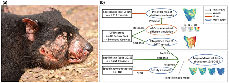
(a) Devil facial tumour disease (DFTD) causes large tumours on the face and mouth of Tasmanian devils (photo: David Hamilton). (b) The main steps involved in our modelling strategy. We first produced maps of the pre-DFTD devil population based on spotlighting data before the discovery of DFTD, and then used this map in a diffusion simulation of DFTD spread across Tasmania (blue box). In a second modelling stage, we used an interpolated map of DFTD spread as a predictor variable in a Bayesian joint-likelihood model, which jointly modelled 35 years of spotlighting data and 21 years of devil density estimates derived from spatially explicit capture-recapture (orange box). From the best joint-likelihood model, we produced maps of devil density, quantified historical changes in the total abundance of the species, and forecasted to the scenario where DFTD will occupy all of the devil’s geographic range.
Early studies indicated that DFTD transmission is strongly frequency-dependent (McCallum et al. 2009), making transmission possible at very low host densities (De Castro & Bolker 2005). This frequency dependence arises because most bite injuries occur during mating interactions when males guard females, which happens irrespective of density (Hamilton et al. 2019). The frequency-dependence led early models to suggest the possibility of disease-induced extinction (McCallum et al. 2009), and consequently, the species was listed as Endangered (Hawkins et al. 2008). While transmission within populations may be maintained by frequency-dependent processes (McCallum et al. 2009), we hypothesise here that the initial spatial spread of DFTD might be a density-dependent process at larger spatial scales.
DFTD now encompasses almost the entire geographic range of the devil (i.e. Tasmania, Australia), presenting the opportunity to study the spread and population effects from the first detection of DFTD to maximum potential distribution. Data are available across the entire range of this emerging host-pathogen system from before and during the early stages of the epizootic. We used three datasets: (1) spatiotemporal occurrences of DFTD, (2) 35 years of spotlighting counts of devils, 10 years prior and 25 years after DFTD discovery, and (3) 21 years of longitudinal capture-mark-recapture host density estimates. Our aims and analysis took a two-stage approach (Fig. 1b). Our first aim was to map and model the spatial spread of DFTD across Tasmania, and to investigate how host density influenced the pattern of disease spread. To do this, we developed a stochastic-diffusion simulation that responded to host density. We parameterised this model using a pattern-oriented framework (Grimm et al. 2005), providing inference on how host density shaped the spatial spread of DFTD. Our second aim was to model the effects of DFTD on devil density and total abundance. Using a map of DFTD spread as an explanatory variable, we jointly modelled the spotlight counts and capture-mark-recapture data. We forecast these findings to the scenario where DFTD occupies the entire range of the devil (Storfer et al. 2017). Finally, we provide the first rigorous estimate of changes in the total abundance of the species.
MATERIALS AND METHODS
Data sources
Spotlight surveys as an index of devil density
The Tasmanian Government has conducted standardised annual spotlighting surveys at up to 172 transects across Tasmania (Fig. 2a; n = 5761) from 1985 to 2019 (Table S1). The surveys record all sightings of non-domestic mammalian wildlife species, including devils (Hocking & Driessen 1992), along 10-km road transects. Transects are driven at a constant speed of 20 km h−1, with one person using a handheld spotlight to observe animals on both sides of the road (for details, see Hocking & Driessen 1992; Hollings et al. 2014). Transects are surveyed once per year during the summer months, ensuring comparability between years, but precluding the use of techniques that require repeat surveys within a year, like occupancy modelling. We treat the count of devils per transect as an index of devil density, and henceforth refer to it as ‘relative density’.
Figure 2.

Maps of study sites and trends in the spotlighting and trapping datasets. (a) The map shows the centroids of each of 172 10-km long spotlight transects. To visualise the broad-scale trends in devil detections, we aggregated transects into the national bioregions (IBRA DSEWPC 2013). The data points show the mean number of devil detections within a bioregion. For visualisation purposes only, the trend lines show the mean estimates from a generalised additive model with 95% confidence band. See Fig. S1 for a finer-scale visualisation of the spotlighting data. (b) Yellow squares show the locations of trapping sites, including those reported by Lazenby et al. (2018) as well as those analysed in this paper. We present four example time-series of devil densities (95% CI) estimated using spatially explicit capture-recapture, with blue and grey points representing densities before and after the arrival of DFTD respectively. The estimates for Bronte, wukalina and Woolnorth come from Lazenby et al. (2018), and we present all density estimates in Fig. S2. In all graphs, the vertical dashed lines denote the approximate year of DFTD arrival to an area. * denotes that disease was discovered at wukalina in 1996, which is earlier than the range of the x-axis.
Estimating absolute density from trapping surveys
We assembled 183 estimates of devil density (±95% CI) derived from standardised 10-day capture-mark-recapture trapping surveys, which used ~ 40 traps set over 25 km2 (Appendix S1, Table S2). We first calculated 87 estimates of devil density using spatially explicit capture-recapture (SECR) models (Borchers & Efford 2008). Since SECR uses the spatial detection history to estimate the effective survey area, it can produce comparable estimates of density across different trap layouts (Borchers & Efford 2008). See Appendix S1 for details. In a second step, we combined our results with 96 estimates of devil density reported by Lazenby et al. (2018), who also used SECR to estimate density. In total, the density estimates came from 72 298 trap nights at 15 sites (Fig. 2B).
Disease spread
We collated records of DFTD locations including those already published from 1996 to 2015 (Lazenby et al. 2018) and recent cases of DFTD in new areas until September 2020. Lazenby et al. (2018) reported locations of lab-confirmed DFTD samples until 2015. We additionally used DFTD locations reported in Hawkins et al. (2006) and McCallum et al. (2007), some of which included cases with clinical signs of DFTD but were not lab-confirmed, which is important before the disease was formally identified. Because we aimed to model the progression of the disease front into new areas, we retained only the earliest arrival of DFTD in each 10 × 10 km2 grid cell across Tasmania, leaving 83 records (Fig. 3).
Figure 3.

After discovery in 1996, the spatial spread of DFTD occurred most rapidly through areas of high devil relative density. The spread of DFTD then appeared to slow as the southern and western disease fronts passed through areas of lower devil relative density. (a) Predictive map of devil spotlighting detections, a proxy for density, at the time of DFTD discovery. This map shows that devils were naturally most abundant in the eastern and central part of Tasmania. The model used data from state-wide spotlight surveys prior to the discovery of DFTD (1985–1996). (b) Map of DFTD spread across Tasmania based on a spatial random field and (c) on a stochastic-diffusion simulation model, incorporating a landscape friction layer based on devil relative density, and parameterised using Approximate Bayesian Computation. The estimated year of disease arrival is shown by colours and contours. Black crosses show the first incidences of lab-confirmed cases of DFTD, or of devils with clinical signs of DFTD. The triangle in the far north-west shows the only remaining long-term trapping site that is currently free of disease, while the squares in the south-west show disease-free areas determined by recent camera trapping. White polygons (b) show inland water bodies. The grey polygon in the south (b) denotes an area with very high uncertainty because of sparse data (standard deviation of at least 3 years; Fig. S4). This area of Tasmania is particularly rugged and has no road access, and consequently very little data from which to infer disease spread.
There is little trapping data from south-west Tasmania because the region is largely inaccessible. To survey this area for DFTD, we used records from recent camera-trap surveys. Although cameras are less sensitive for detecting small tumours, they regularly detect tumours when they become larger. In this case, cameras observed tumours in areas with confirmed cases of DFTD but did not detect DFTD along the south-west coast (2016–2020), where live trapping in 2015 also did not detect DFTD. We have therefore included eight absence locations along the south-west coast (Fig. 3). Additionally, one long-term trapping site in the north-west is currently free of disease (Fig. 3). Based on a continuation of the pattern of spread, we estimated that DFTD would arrive at these disease-free sites in 2022 (Fig. 3B). Future disease spread may differ from this estimate, but any departures will have only a small effect on the population estimates because the influence of these data points relates to a small, low-density area of Tasmania.
Modelling spatial data using integrated nested Laplace approximation
We visualised the spatial spread of DFTD and modelled changes in devil density using integrated nested Laplace approximation (INLA) (Illian et al. 2013), an accurate and computationally fast option for Bayesian inference from spatial data. We used the inlabru R package (Bachl et al. 2019; R Core Team 2019), which builds on the R-INLA package (Rue et al. 2009; Bakka et al. 2018). Spatial dependence between observations is modelled using a Gaussian random field, which is a spatially continuous process where random variables at any point in space are normally distributed, and are spatially correlated with other random points via a continuous correlation process (Bachl et al. 2019). The Gaussian random field is approximated by a stochastic partial differential equation (SPDE) (for details, see Lindgren et al. 2011). In all models, we used a Matérn correlation structure for the SPDE (Table S6).
Modelling the pre-DFTD devil population
We spatially modelled devil relative density at the time of DFTD discovery using the count of devils per spotlight transect from 1985 to 1996 as the response variable. We created temporally static continuous variables for the proportional cover of four major habitat classes comprising 84% of Tasmania: (1) wet eucalypt and rainforest (%wetEuc, 28% of Tasmania), (2) dry eucalypt forest (%dryEuc, 24%), (3) buttongrass moorlands (%butGrass, 9%), and (4) agricultural land (%agric, 23%). We excluded %dryEuc from the models because it was negatively correlated with %wetEuc (Pearson’s r = −0.65). We modelled a non-linear effect of ‘survey year’ (1985–1996) using a one-dimensional SPDE. Finally, to model spatial correlations not accounted for by covariates, as well as correlations between repeated surveys at a location, we created (1) a temporally static two-dimensional SPDE and (2) a spatiotemporal SPDE. See Table S6 for details and ecological justification of these variables and Fig. S1 for a vegetation map.
We followed the model selection advice of Illian et al. (2013) when inferring the effect of spatial covariates in models that also include spatial random fields. We began by fitting a model with the three vegetation covariates and ‘survey year’. Using this model, we tested whether devil counts best conformed to a Poisson or negative binomial distribution. Then, we fitted all simpler combinations of the vegetation covariates, aiming to select the statistically important vegetation covariates. Next, we added a temporally static SPDE, and finally a spatiotemporal SPDE (see Table S7 for models). We selected the best model using a leave-one-out cross-validation quantity, the conditional predictive ordinate (CPO), with smaller values of −2 × Σ(logCPO) indicating better fit (Pettit 1990). To screen for violations of assumptions, we spatially examined CPO scores and histograms of the predictive integral transform, and visually examined Pearson residuals against model estimates (Conn et al. 2018). From the best model, we produced a predictive map of devil relative density across Tasmania as a function of the vegetation covariates and random field, with year set to 1996. We did this using the predict function of inlabru, which repeatedly draws samples from the posterior distributions of the model parameters.
Pattern-oriented diffusion simulation of the spatial spread of DFTD
To investigate the effect of host density on the spatial spread of DFTD, we developed a grid-based, stochastic-diffusion simulation. We parameterised this model using a pattern-oriented framework, which provides a systematic, data-oriented way of calibrating complex simulation models (Grimm et al. 2005; Grimm & Railsback 2012). Specifically, we used Approximate Bayesian Computation (ABC) using the abc package (Csilléry et al. 2012) in R. This involved running many versions of the model, each with different parameters drawn from vaguely specified prior distributions. Using summary statistics from the simulations, ABC selects only the models that are close to reproducing ‘target’ statistics calculated from the observed data, from which ABC estimates the posterior parameter distributions (Csilléry et al. 2010; Csilléry et al. 2012).
To initiate the simulation, we seeded one grid cell in north-east Tasmania with DFTD at a location between the first two observed cases of DFTD. We started the simulation in 1990 because genomic evidence suggests that although DFTD probably emerged in the 1980s, it was not until the mid-1990s that the effective reproduction number increased and DFTD began to spread more widely (Patton et al. 2020). In each of 31 time-steps (1990–2020), the probability of DFTD spreading into an unoccupied grid cell was first determined by the distance, s, from an occupied cell. For cells within s distance, the odds, Y, of DFTD spreading into a cell was:
where β1 is an intercept and β2 is a coefficient for the effect of devil relative density (previous section). The probability of diffusing into a new cell was stochastically determined by sampling from the binomial distribution with a probability of exp (Y)/(1 + exp(Y)). We assumed that once grid cells were infected by DFTD, they remained so thereafter, which is broadly true at the landscape scale.
We used ABC to estimate the posterior distributions of s, β1 and β2. We considered parameters for β1 and β2 to be important if credible intervals did not span zero. We evaluated the simulations on their ability to correctly estimate the year of arrival at 83 DFTD locations and the absence of DFTD in 9 DFTD-free locations. See Appendix S2 for model details and see Appendix S3 for R code.
To visually compare the results of the ABC-parameterised simulation with the observed data, we created an interpolated map of DFTD first cases. Using inlabru (Bachl et al. 2019) in R, we modelled the year of DFTD arrival using a Gaussian distribution in response to a spatial random field only (Table S6). From this model, we produced a smooth map of estimated disease-arrival times. Because this model is based solely on a spatial random field, it provides no direct inference about the processes responsible for the pattern of disease spread. Nevertheless, because it directly fits the data, it has higher descriptive fidelity than the diffusion model. We therefore use the diffusion model to interpret the processes driving DFTD spread, while using the random-field-map for the subsequent models investigating population effects.
Integrating multiple data sources into a joint-likelihood model
We integrated the density and spotlight datasets into a Bayesian joint-likelihood model. Joint likelihood models combine multiple data sources into single integrated models that estimate a shared set of parameters (Miller et al. 2019; Isaac et al. 2020). The integrated model has sub-models for each data source, with some or all parameters shared between the sub-models (Bachl et al. 2019; Miller et al. 2019). We fitted the joint-likelihood model using the inlabru R package (tutorials in Bachl et al. 2019; Watson et al. 2019). To model spatiotemporal changes to devil density from the spotlighting and density datasets, we created explanatory variables for ‘survey year’ (1985–2019) and the model-estimated number of years since DFTD arrival to a site (‘yrsDFTD’; 0–23 years), which we estimated from the random-field-map of disease spread (Fig. 3B). Non-linear effects of ‘survey year’ and ‘yrsDFTD’ were modelled using one-dimensional SPDEs (Table S6). As previously described, we modelled the effect of three vegetation types: %wetEuc, %agric and %butGrass. Finally, to model spatial correlations not accounted for by covariates, we included in separate models a temporally static two-dimensional SPDE and a spatiotemporal SPDE that allows the random field to change through time (Table S6).
We followed the same model selection process as for the pre-DFTD model, first by selecting the important environmental covariates, and then adding spatial random fields (Illian et al. 2013). For the spotlighting sub-model, the response variable was the count of devils observed on a transect (Poisson or negative binomial distribution). For the density sub-model, the response variable was the estimated devil density for each trapping session (devils/km2; gamma or Weibull distribution). All models used the default link function. The most complex joint-likelihood model took the form of
where β1 and β2 are intercepts for each sub-model, f3 and f4 are shared non-linear effects, β5, β6, β7 are shared fixed effects, SPDE is a shared spatial random field and β8 is a scaling constant that modifies f3 (see chapter 3 of Krainski et al. 2019). We included the scaling constant because initial exploration of the two datasets suggested that the spotlight data slightly overstated the decline in devil density. See Table S9 for the structure of all fitted models. From the density sub-model of the best joint model, we produced predictive maps of devil density across Tasmania at various points from 1985 to 2035 (predict function of inlabru). To estimate the total devil abundance, we multiplied density estimates weighted by the area of each grid location across Tasmania. See Appendix S4 for example R code.
RESULTS
Density-dependent spatial spread of DFTD
Devil relative density varied substantially across Tasmania at the time of DFTD discovery (Fig. 3A). The best model of pre-DFTD spotlight detections included a spatiotemporal random field and negative effects of wet eucalypt/rainforest and buttongrass (Table S7). As a result, devil relative density was highest in the central and eastern part of Tasmania, where vegetation is dominated by dry eucalypt forests and woodlands (Fig. 3A).
The diffusion simulation of DFTD spread suggests that devil density played a key role in mediating the initial spatial spread of DFTD. Within a timestep, the ABC posteriors estimated that DFTD was able to diffuse into grid cells within ~ 18 km of already-occupied cells, with the probability of doing so strongly influenced by the relative devil density of the receiving grid cell (βrelativeDensity = 7.75, 95% CI: 6.89-8.29) (Table S8; Fig. S5). This model goes some way to explain why DFTD spread south rapidly in the decade after ‘break-out’, as it moved through an area with high relative densities (Fig. 3). From the mid-2000s, the spread of DFTD was substantially slower, as the western and southern disease-fronts crossed areas of lower relative densities (Fig. 3). The diffusion model correctly predicted that much of south-west Tasmania, a rugged area with low devil densities (Hawkins et al. 2006), is currently free of DFTD. The diffusion model and random-field-model estimate that DFTD occupies 91% and 96% of Tasmania (Fig. 3) respectively, with high uncertainty in southern Tasmania, where data is sparse (Fig. S4).
Devil population declines
The joint-likelihood model revealed a strong negative effect of ‘yrsDFTD’, with local devil densities declining by an average of 76% 10 years after disease arrival, at which point the population decline tends to level off, with 82% decline after 23 years (Fig. 4C). The joint model revealed a positive effect of ‘survey year’, and negative effects of %butGrass and %wetEuc (Fig. 4; Table 1; Fig. S6). Devil density was steadily rising before the discovery of DFTD, peaking in 1996 at a Tasmania-wide mean of 0.84 devils/km2 (95% CI: 0.61–1.08) and a total population of 53 000 (95% CI: 39 600–71 800) (Fig. 5). By 2020, estimated mean density had declined to 0.27/km2 (0.20–0.36) and the total population had declined by 68% to 16 900 (12 500–23 100) (Fig. 5).
Figure 4.

(a) Predictive maps of Tasmanian devil density from the joint-likelihood model. Devil densities were rising before the discovery of DFTD in 1996. The spread of DFTD across Tasmania then caused a wave of rapid and severe population declines. In the first panel (only), black dots indicate the location of annual spotlight transects and maroon squares show the location of longitudinal trapping sites. See Fig. S7 for maps of uncertainty around the density estimates. (b–e) The effect of predictor variables on devil density from the best joint-likelihood model (±95% credible interval). Grey lines show the effect of a predictor variable across its range when all other predictors are held at their mean (i.e. 4.5 years after the arrival of DFTD), and yellow lines show the effect when sites were free of DFTD. The axis ranges reflect the range of those variables.
Table 1.
Model selection table for the joint-likelihood model, which simultaneously modelled devil density at long-term trapping sites and devil detections on long-term spotlight transects. Here we present the four top-performing models and a null model. We selected the best model based on a leave-one-out cross-validation metric, the conditional predictive ordinate (CPO), with ΔCPO showing the difference from the best model. We present the mean coefficient estimate, with 95% credible interval shown in brackets. ‘nl’ denotes a non-linear effect. All models in this table used the gamma distribution to model density and the negative binomial distribution to model the spotlight counts. See Table S9 for the full model selection table
| Model | −2 × Σ(logCPO) |
ΣCPO | Intercept: spotlight sub-model |
Intercept: density sub-model |
Year | Years since DFTD arrival |
Scaling constant |
% button grass |
% wet eucalypt/ rainforest |
% agric | Gaussian random field |
|---|---|---|---|---|---|---|---|---|---|---|---|
| 1 | 7570.5 | 0.0 |
2.61
(−3.46, −1.92) |
−1.58
(−2.3, −0.96) |
nl | nl |
0.70
(0.59, 0.81) |
−1.88
(−3.65, −0.19) |
−0.80
(−1.37, −0.24) |
✓ | |
| 2 | 7571.2 | 0.7 | −2.59 (−3.48, −1.86) |
−1.57 (−2.31, −0.91) |
nl | nl | 0.70 (0.59, 0.81) |
−1.91 (−3.71, −0.18) |
−0.82 (−1.43, −0.20) |
−0.05 (−0.67, 0.57) |
✓ |
| 3 | 8036.3 | 465.8 | −2.64 (−3.80, −1.94) |
−1.53 (−2.42, −0.94) |
nl | nl | 0.76 (0.62, 0.89) |
−1.05 (−1.74, −0.37) |
−0.86 (−1.07, −0.65) |
0.27 (0.01, 0.54) |
|
| 4 | 8038.7 | 468.1 | −2.57 (−3.75, −1.86) |
−1.48 (−2.41, −0.88) |
nl | nl | 0.78 (0.64, 0.92) |
−1.28 (−1.94, −0.61) |
−0.93 (−1.14, −0.73) |
||
| Null | 8884.5 | 1314.0 | −1.07 (−1.12, −1.01) |
−0.49 (−0.60, −0.37) |
Figure 5.

Changes in the Tasmanian devil population across the entire geographic range of the species. (a) Estimates of devil density across Tasmania at time points from 1985 and 2030. Yellow bars distinguish density in areas that are free of DFTD and grey shows densities where DFTD is present. The vertical dashed lines show the mean density in each disease category, with black denoting the overall mean. (b) Changes in the global abundance (±95% credible interval) of Tasmanian devils. Dashed lines represent forecasts into the future. The black line shows the estimated proportion of Tasmania occupied by DFTD based on the random-field-model of disease spread (Fig. 3b).
To project forward to the scenario where DFTD will occupy all of Tasmania, we made the simplifying assumption, based on a continuation of disease spread trends, that DFTD will occupy all of Tasmania by 2022. Based on this assumption, our model forecasts a continuing but slowing decline of total devil abundance (Fig. 5), suggesting it should plateau at 11 900 devils (95% CI: 6300–18 600). Overall, this would represent a 78% decline in total abundance. To date, no local extinctions have been documented, with devil populations persisting at all monitoring sites, albeit at much lower densities (Fig. S2).
DISCUSSION
We modelled the spread of an infectious epizootic disease, DFTD, from emergence until the present, where it now occupies > 90% of the geographic range of its sole host, the Tasmanian devil. DFTD emerged in an area of high host density, potentially creating the perfect conditions for the epizootic to establish and spread, with our diffusion simulation suggesting that DFTD spread fastest in areas of high host density. We integrated 35 years of spotlighting data and 21 years of capture-mark-recapture data to spatially model changes in the devil population, highlighting the utility of recent advances in data integration for modelling changes to species’ distributions (Miller et al. 2019; Isaac et al. 2020). The joint-likelihood model allowed us to quantify, for the first time, the wave of severe population declines as DFTD invaded host populations. Our forecast, which does not include rapid evolutionary dynamics, predicts the devil population decline is likely to level-off within the next decade.
Density-dependent spatial spread of DFTD
Our pattern-oriented diffusion simulation suggests that DFTD spread most rapidly through areas of high host density. This raises an interesting point about spatial scale: although transmission within devil populations may be maintained by frequency-dependent processes (McCallum et al. 2009), the spatial spread of DFTD was apparently density-dependent. Using a simple diffusion model, van den Bosch et al. (1992) show that the spread of an invading organism is driven by a combination of the host movement rate and the intrinsic rate of increase. Both movement rate and interactions between devils could increase in response to competition. At high devil densities, carrion and live prey are less available per capita (Cunningham et al. 2018) and aggressive interactions at carcasses are more common (Hamede et al. 2008). Female devils in high density populations have larger home ranges (Comte et al. 2020) and disperse larger distances (Lachish et al. 2011; Storfer et al. 2017). Other studies, for instance of European badgers, show that larger home ranges can lead to increased potential for pathogen transmission (Woodroffe et al. 2006), and simulations show that greater host movement can increase the probability of a pandemic establishing (Cross et al. 2005). Adult devils sometimes engage in long-distance excursions of ~ 15–25 km (M. Jones, unpublished tracking data). These are likely to be more numerous at high densities, and could act as rare long-distance transmission events, which have been shown in other systems to substantially accelerate disease spread (Smith et al. 2002; Russell et al. 2005; Smith et al. 2005; Meentemeyer et al. 2011). Our simulation model was a first step in establishing a probable link between host density and the spatial spread of DFTD. Future studies should unpick the mechanisms that depend on density, and incorporate other drivers or barriers of DFTD spread, both of which would likely require a finer scale of study that matches the scale of transmission and host movement.
Population trends and conservation
Our estimate of pre-DFTD devil population size is less than half the previous estimate of 130 000–150 000 (Hawkins et al. 2008), which would require average densities across Tasmania of 2.15 devils/km2. Our estimates suggest that only 1.3% of Tasmania had densities of at least 2.15 devils/km2 at the time of DFTD discovery (Fig. 5B). This discrepancy might have two main causes. First, SECR has produced smaller density estimates than older methods. SECR uses the spatial detection histories of animals to estimate the effective sampling area (Borchers & Efford 2008), which can differ substantially between similar-sized trapping arrays (Table S5). In contrast, older methods defined the sampling area based on a buffer around trap sites without considering how animal movement around study sites influences the effective survey area (Hawkins et al. 2008). Second, previous extrapolations seemingly suffered from a common form of site selection bias, whereby study sites are selected in high-density areas (Fournier et al. 2019). Extrapolating such density estimates to areas with lower suitability, such as the Tasmanian south-west (Jones & Rose 1996; Hawkins et al. 2006), is likely to result in an over-estimated population size. The integration of multiple datasets in our analysis allowed us to incorporate information from a broader range of environments, including low-suitability habitat, while harnessing the favourable qualities of each dataset (high-quality density estimates and long-term, wide-spread spotlight counts).
Based on the persistence of devils at all long-term diseased sites, our model predicts the overall population is likely to stabilise within the next 10 years. This supports recent simulations suggesting the most likely long-term outcomes are either the coexistence of devils and DFTD, or DFTD fading out (Wells et al. 2019), with genomic evidence suggesting a transition towards endemism (Patton et al. 2020). These stabilising trends reflect a growing body of research suggesting that devils are potentially adapting to DFTD in the face of this extreme selective pressure (Epstein et al. 2016; Ruiz-Aravena et al. 2018; Margres et al. 2018a; Fraik et al. 2020). Several individual devils have demonstrated natural tumour regressions in association with an immune response (Pye et al. 2016a), with tumour regression potentially related to genomic variation in both host (Margres et al. 2018b) and tumour (Margres et al. 2020). Nevertheless, it remains unclear how the genomic changes detected in long-term diseased areas (Epstein et al. 2016) relate to functional traits in devil-DFTD interactions, and whether genomic changes are involved in the persistence and even recovery of some populations.
Despite revealing 25 years of ongoing population decline, our results suggest the species no longer meets the criteria for Endangered status under the IUCN Red List. Because the Red List evaluates population reductions over the longer of 10 years or three generations (IUCN Standards & Petitions Committee 2019), the severe devil population decline before 2010 is essentially excluded from consideration. Our modelling suggests the species now qualifies for Vulnerable status based on a 31% population decline from 2011 to 2020 (criterion A2), and a reproductively mature population size that is likely to be < 10 000 but > 2500 individuals within the next decade (criterion C1). Given the population has declined by 68% over the last 25 years, numbers continue to decline, and the trend is not reversible with current knowledge, we strongly caution that the potential down-listing of the species does not mean the species is secure. This is particularly so in the face of new and uncertain threats, including the discovery in 2014 of a second, independently evolved facial tumour (DFT2) which is spreading through southern Tasmania (Pye et al. 2016b; James et al. 2019).
Although the outlook for the wild devil population is undoubtedly more positive than it was a decade ago (McCallum et al. 2009), devils are currently well below ecologically functional densities across much of Tasmania. Devil declines have had cascading ecological effects, such as carrion accumulation (Cunningham et al. 2018), mesopredator release with effects on small and medium-sized mammals (Hollings et al. 2014; Hollings et al. 2016; Cunningham et al. 2020), and the relaxation of anti-predator behaviours by prey (Hollings et al. 2015; Cunningham et al. 2019a; Cunningham et al. 2019b). In the the online data repository, we provide annual rasters of estimated devil densities from 1985 to 2035, which we expect will be useful for improving our understanding of the ecological effects of devils and identifying thresholds that could provide longer term targets for population recovery.
Given DFTD-induced extinction of the devil now seems unlikely, we suggest several management priorities. First, we emphasise the importance of continued monitoring across the species’ geographic range, particularly following the discovery of DFT2 (Pye et al. 2016b). Second, because the now-small devil population is more exposed to other threatening processes (De Castro & Bolker 2005; McCallum 2012), it is an ongoing priority to minimise additional stressors like vehicle collisions and habitat destruction. A third exciting priority is that we can attempt to accelerate the pace of evolution by identifying and then moving advantageous genotypes to areas lacking them (McCallum 2012). Crucially, these genotypes need to come from populations that are under selective pressure by DFTD (Hohenlohe et al. 2019; Hamede et al. 2020). It is, however, important to recognise the potential for DFTD to evolve in response to changes in the host population, and that selecting for resistant devils might inadvertently select for more virulent tumours. Before intervening to boost adaptation, it is therefore important to better understand (1) how genotype influences phenotype in both devils and DFTD, and (2) how these traits influence the persistence of devils in long-diseased populations.
Concluding remarks
Modelling spatial dynamics of pathogens in wildlife populations remains a major challenge (White et al. 2018), but is critical for managing emerging disease threats, both to wildlife themselves and to human or livestock populations to which these pathogens may spill over. Our study of DFTD as it has spread across almost the entire geographic range of its sole host takes advantage of recent advances in pattern-oriented modelling, as well as joint modelling of multiple datasets. Diffusion-based approaches are often considered to be high-level general frameworks not well suited to providing specific predictions (White et al. 2018). By re-imagining a diffusion model as a multi-layer, grid-based simulation, our framework can accommodate complex processes that would otherwise be intractable using an analytical diffusion model. Our highly flexible simulation shows that diffusion-based models can provide explicit quantitative information on the relationship between host density and spatial spread, which should have broad, real-world applications to other wildlife disease systems, and invading organisms more generally. Ours is, however, one of few studies of emerging infectious diseases with plentiful ‘spatiotemporal data on both host and pathogen populations from the time of disease emergence. This high-lights the importance of long-term monitoring programs. Regular, joint analysis of general-purpose survey datasets that monitor a large suite of species would be valuable for the early detection of population declines or disease emergence at a point where management interventions can be effective. Our analysis involved the use of survey data that was established to monitor harvested herbivore species, but has now provided valuable insights into the influence of host density on infectious disease spread and the population effects of an emerging infectious disease that did not exist when the surveys were established.
Supplementary Material
ACKNOWLEDGEMENTS
The manuscript was made possible by two bequests to the UTAS University Foundation Save the Tasmanian Devil Appeal, from The Estate of the late Pauline Barnett and The Estate of the late Nancy Frederiksen, which supported CXC as a postdoctoral fellow. Field work was supported by NIH Grant R01-GM126563-01 and NSF Grant DEB 1316549 to A.S., P.A.H., M.E.J. and H.M. as part of the joint NIH-NSF-USDA Ecology and Evolution of Infectious Diseases program, the Australian Research Council (ARC) Future Fellowship (FT100100250) to M.J., ARC Large Grants (A00000162) to M.J., Linkage (LP0561120, LP0989613) to M.J. and H.M., Discovery (DP110102656) to M.J. and H.M., DECRA (170101116) and Linkage (LP170101105) to R.H., multiple Holsworth Wildlife Trust, Eric Guiler Grants (UTAS Foundation Save the Tasmanian Devil Appeal) and Estate of WV Scott grants, and grants from the National Geographic Society, Mohammed bin Zayed Conservation Fund, Ian Potter Foundation and Australian Academy of Science. Field work was supported by innumerable volunteers and was conducted with permission and field support from the Tasmanian Parks and Wildlife Service and Forico Pty Ltd. We thank the Tasmanian Department of Primary Industries, Parks, Water and Environment for providing access to the spotlighting dataset, and Billie Lazenby for early discussions around the analysis, and four anonymous reviewers for constructive reviews.
Footnotes
ETHICS STATEMENT
This study was conducted in accordance with the Univ. of Tasmania Animal Ethics Committee permits A0008588, A0010296, A0011696, A0013326, A0015835, A0018223 and A0016789.
SUPPORTING INFORMATION
Additional supporting information may be found online in the Supporting Information section at the end of the article.
DATA AVAILABILITY STATEMENT
The data supporting the results have been archived in the Dryad public data repository (https://doi.org/10.6084/m9.figshare.13624406.v1; https://doi.org/10.6084/m9.figshare.13624517.v1; https://doi.org/10.6084/m9.figshare.13624565.v1; https://doi.org/10.6084/m9.figshare.13728220).
REFERENCES
- Anderson RM & May RM (1979). Population biology of infectious diseases: Part I. Nature, 280, 361–367. [DOI] [PubMed] [Google Scholar]
- Bachl FE, Lindgren F, Borchers DL & Illian JB (2019). inlabru: an R package for Bayesian spatial modelling from ecological survey data. Methods Ecol. Evol, 10, 760–766. [Google Scholar]
- Bakka H, Rue H, Fuglstad G-A, Riebler A, Bolin D, Illian J et al. (2018). Spatial modeling with R-INLA: a review. WIREs Computational Statistics, 10, e1443. [Google Scholar]
- Borchers DL & Efford MG (2008). Spatially explicit maximum likelihood methods for capture-recapture studies. Biometrics, 64, 377–385. [DOI] [PubMed] [Google Scholar]
- van den Bosch F, Hengeveld R & Metz JAJ (1992). Analysing the velocity of animal range expansion. J. Biogeogr, 19, 135–150. [Google Scholar]
- van den Bosch F, Metz JAJ & Diekmann O (1990). The velocity of spatial population expansion. J. Math. Biol, 28, 529–565. [Google Scholar]
- Buck JC & Ripple WJ (2017). Infectious agents trigger trophic cascades. Trends Ecol. Evol, 32, 681–694. [DOI] [PubMed] [Google Scholar]
- Comte S, Carver S, Hamede R & Jones M (2020). Changes in spatial organization following an acute epizootic: Tasmanian devils and their transmissible cancer. Glob. Ecol. Conserv, 22, e00993. [DOI] [PMC free article] [PubMed] [Google Scholar]
- Conn PB, Johnson DS, Williams PJ, Melin SR & Hooten MB (2018). A guide to Bayesian model checking for ecologists. Ecol. Monogr, 88, 526–542. [Google Scholar]
- Cross PC, Lloyd-Smith JO, Johnson PLF & Getz WM (2005). Duelling timescales of host movement and disease recovery determine invasion of disease in structured populations. Ecol. Lett, 8, 587–595. [Google Scholar]
- Csilléry K, Blum MGB, Gaggiotti OE & François O (2010). Approximate Bayesian Computation (ABC) in practice. Trends Ecol. Evol, 25, 410–418. [DOI] [PubMed] [Google Scholar]
- Csilléry K, François O & Blum MGB (2012). abc: an R package for approximate Bayesian computation (ABC). Methods Ecol. Evol, 3, 475–479. [Google Scholar]
- Cunningham CX, Johnson CN, Barmuta LA, Hollings T, Woehler E & Jones ME (2018). Top carnivore decline has cascading effects on scavengers and carrion persistence. Proc. R. Soc. B, 285, 20181582. [DOI] [PMC free article] [PubMed] [Google Scholar]
- Cunningham CX, Johnson CN, Hollings T, Kreger K & Jones ME (2019a). Trophic rewilding establishes a landscape of fear: Tasmanian devil introduction increases risk-sensitive foraging in a key prey species. Ecography, 42(12), 2053–2059. [Google Scholar]
- Cunningham CX, Johnson CN & Jones ME (2020). A native apex predator limits an invasive mesopredator and protects native prey: Tasmanian devils protecting bandicoots from cats. Ecol. Lett, 23(4), 711–721. [DOI] [PubMed] [Google Scholar]
- Cunningham CX, Scoleri V, Johnson CN, Barmuta LA & Jones M (2019b). Temporal partitioning of activity: rising and falling top-predator abundance triggers community-wide shifts in diel activity. Ecography, 42(12), 2157–2168. [Google Scholar]
- Daszak P, Cunningham AA & Hyatt AD (2000). Emerging infectious diseases of wildlife– threats to biodiversity and human health. Science, 287, 443–449. [DOI] [PubMed] [Google Scholar]
- De Castro F & Bolker B (2005). Mechanisms of disease-induced extinction. Ecol. Lett, 8, 117–126. [Google Scholar]
- Dobson A & Foufopoulos J (2001). Emerging infectious pathogens of wildlife. Philos. Trans. R. Soc. Lond. B Biol. Sci, 356, 1001–1012. [DOI] [PMC free article] [PubMed] [Google Scholar]
- Dobson A & Hudson P (1995). Microparasites: observed patterns in wild animal populations. In: Ecology of infectious diseases in natural populations (eds. Grenfell B & Dobson A). Cambridge University Press, Cambridge, p. 89. [Google Scholar]
- Epstein B, Jones M, Hamede R, Hendricks S, McCallum H, Murchison EP et al. (2016). Rapid evolutionary response to a transmissible cancer in Tasmanian devils. Nat. Commun, 7, 12684. [DOI] [PMC free article] [PubMed] [Google Scholar]
- Fletcher RJ Jr, Hefley TJ, Robertson EP, Zuckerberg B, McCleery RA & Dorazio RM (2019). A practical guide for combining data to model species distributions. Ecology, 100, e02710. [DOI] [PubMed] [Google Scholar]
- Fournier AMV, White ER & Heard SB (2019). Site-selection bias and apparent population declines in long-term studies. Conserv. Biol, 33, 1370–1379. [DOI] [PubMed] [Google Scholar]
- Fraik AK, Margres MJ, Epstein B, Barbosa S, Jones M, Hendricks S et al. (2020). Disease swamps molecular signatures of genetic-environmental associations to abiotic factors in Tasmanian devil (Sarcophilus harrisii) populations. Evolution, 74(7), 1392–1408. [DOI] [PMC free article] [PubMed] [Google Scholar]
- Grimm V & Railsback SF (2012). Pattern-oriented modelling: a multi-scope for predictive systems ecology. Philos. Trans. R. Soc. Lond. B Biol. Sci, 367, 298–310. [DOI] [PMC free article] [PubMed] [Google Scholar]
- Grimm V, Revilla E, Berger U, Jeltsch F, Mooij WM, Railsback SF et al. (2005). Pattern-oriented modeling of agent-based complex systems: lessons from ecology. Science, 310, 987. [DOI] [PubMed] [Google Scholar]
- Hagenaars TJ, Donnelly CA & Ferguson NM (2004). Spatial heterogeneity and the persistence of infectious diseases. J. Theor. Biol, 229, 349–359. [DOI] [PubMed] [Google Scholar]
- Hamede R, Madsen T, McCallum H, Storfer A, Hohenlohe PA, Siddle H et al. (2020) Darwin, the devil, and the management of transmissible cancers. Conservation Biology, 10.1111/cobi.13644. [DOI] [PMC free article] [PubMed] [Google Scholar]
- Hamede RK, McCallum H & Jones M (2008). Seasonal, demographic and density-related patterns of contact between Tasmanian devils (Sarcophilus harrisii): Implications for transmission of devil facial tumour disease. Austral Ecol, 33, 614. [Google Scholar]
- Hamilton DG, Jones ME, Cameron EZ, McCallum H, Storfer A, Hohenlohe PA et al. (2019). Rate of intersexual interactions affects injury likelihood in Tasmanian devil contact networks. Behav. Ecol, 30 (4), 1087–1095. [Google Scholar]
- Hawkins CE, Baars C, Hesterman H, Hocking GJ, Jones ME, Lazenby B et al. (2006). Emerging disease and population decline of an island endemic, the Tasmanian devil Sarcophilus harrisii. Biol. Cons, 131, 307–324. [Google Scholar]
- Hawkins CE, McCallum H, Mooney N, Jones M & Holdsworth M (2008). Sarcophilus harrisii. The IUCN Red List of Threatened Species; 2008: e.T40540A10331066. 10.2305/IUCN.UK.2008.RLTS.T40540A10331066.en. [DOI] [Google Scholar]
- Hocking GJ & Driessen MM (1992). Tasmanian Spotlight Survey Manual: A Set of Instructions and Maps for Conducting Spotlight Surveys in Tasmania. Department of Parks Wildlife and Heritage, Hobart. [Google Scholar]
- Hohenlohe PA, McCallum HI, Jones ME, Lawrance MF, Hamede RK & Storfer A (2019). Conserving adaptive potential: lessons from Tasmanian devils and their transmissible cancer. Conserv. Genet, 20, 81–87. [DOI] [PMC free article] [PubMed] [Google Scholar]
- Hollings T, Jones M, Mooney N & McCallum H (2014). Trophic cascades following the disease-induced decline of an apex predator, the Tasmanian devil. Conserv. Biol, 28, 63–75. [DOI] [PubMed] [Google Scholar]
- Hollings T, Jones M, Mooney N & McCallum HI (2016). Disease-induced decline of an apex predator drives invasive dominated states and threatens biodiversity. Ecology, 97, 394–405. [DOI] [PubMed] [Google Scholar]
- Hollings T, McCallum H, Kreger K, Mooney N & Jones M (2015). Relaxation of risk-sensitive behaviour of prey following disease-induced decline of an apex predator, the Tasmanian devil. Proc. R. Soc. B, 282, 20150124. [DOI] [PMC free article] [PubMed] [Google Scholar]
- Hosseini PR, Dhondt AA & Dobson AP (2006). Spatial spread of an emerging infectious disease: conjunctivitis in house finches. Ecology, 87, 3037–3046. [DOI] [PubMed] [Google Scholar]
- IBRA DSEWPC (2013). Interim Biogeographic Regionalisation for Australia (IBRA), Version 7 (Regions). [Google Scholar]
- Illian JB, Martino S, Sørbye SH, Gallego-Fernández JB, Zunzunegui M, Esquivias MP et al. (2013). Fitting complex ecological point process models with integrated nested Laplace approximation. Methods Ecol. Evol, 4, 305–315. [Google Scholar]
- Isaac NJB, Jarzyna MA, Keil P, Dambly LI, Boersch-Supan PH, Browning E et al. (2020). Data integration for large-scale models of species distributions. Trends Ecol. Evol, 35, 56–67. [DOI] [PubMed] [Google Scholar]
- IUCN Standards and Petitions Committee (2019). Guidelines for Using the IUCN Red List Categories and Criteria. http://www.iucnredlist.org/documents/RedListGuidelines.pdf. [Google Scholar]
- James S, Jennings G, Kwon YM, Stammnitz M, Fraik A, Storfer A et al. (2019). Tracing the rise of malignant cell lines: Distribution, epidemiology and evolutionary interactions of two transmissible cancers in Tasmanian devils. Evol. Appl, 12, 1772–1780. [DOI] [PMC free article] [PubMed] [Google Scholar]
- Jones ME & Rose RK (1996). Preliminary Assessment of Distribution and Habitat Associations of the Spotted-Tailed Quoll (Dasyurus maculatus maculatus) and Eastern Quoll (D. viverrinus) in Tasmania to Determine Conservation and Reservation Status. Tasmanian Public Land Use Commission, Hobart, Tasmania. [Google Scholar]
- Krainski ET, Gómez-Rubio V, Bakka H, Lenzi A, Castro-Camilo D, Simpson D et al. (2019). Chapter 3: More than one likelihood. In: Advanced Spatial Modeling with Stochastic Partial Differential Equations Using R and INLA. CRC Press/Taylor and Francis Group. https://becarioprecario.bitbucket.io/spde-gitbook/ch-manipula.html. [Google Scholar]
- Lachish S, Miller KJ, Storfer A, Goldizen AW & Jones ME (2011). Evidence that disease-induced population decline changes genetic structure and alters dispersal patterns in the Tasmanian devil. Heredity, 106, 172–182. [DOI] [PMC free article] [PubMed] [Google Scholar]
- Langwig KE, Voyles J, Wilber MQ, Frick WF, Murray KA, Bolker BM et al. (2015). Context-dependent conservation responses to emerging wildlife diseases. Front. Ecol. Environ, 13, 195–202. [Google Scholar]
- Lazenby BT, Tobler MW, Brown WE, Hawkins CE, Hocking GJ, Hume F et al. (2018). Density trends and demographic signals uncover the long-term impact of transmissible cancer in Tasmanian devils. J. Appl. Ecol, 55, 1368–1379. [DOI] [PMC free article] [PubMed] [Google Scholar]
- Lindgren F, Rue H & Lindström J (2011). An explicit link between Gaussian fields and Gaussian Markov random fields: the stochastic partial differential equation approach. J. R. Stat. Soc. Series B Stat. Methodol, 73, 423–498. [Google Scholar]
- Margres MJ, Jones ME, Epstein B, Kerlin DH, Comte S, Fox S et al. (2018a). Large-effect loci affect survival in Tasmanian devils (Sarcophilus harrisii) infected with a transmissible cancer. Mol. Ecol, 27, 4189–4199. [DOI] [PMC free article] [PubMed] [Google Scholar]
- Margres MJ, Ruiz-Aravena M, Hamede R, Jones ME, Lawrance MF, Hendricks SA et al. (2018b). The genomic basis of tumor regression in Tasmanian Devils (Sarcophilus harrisii). Genome Biology and Evolution, 10, 3012–3025. [DOI] [PMC free article] [PubMed] [Google Scholar]
- Margres MJ, Ruiz-Aravena M, Hamede R, Chawla K, Patton AH, Lawrance MF et al. (2020). Spontaneous tumor regression in Tasmanian devils associated with RASL11A activation. Genetics, 215 (4), 1143–1152. [DOI] [PMC free article] [PubMed] [Google Scholar]
- McCallum H (2012). Disease and the dynamics of extinction. Philos. Trans. R. Soc. B Biol. Sci, 367, 2828–2839. [DOI] [PMC free article] [PubMed] [Google Scholar]
- McCallum H, Barlow N & Hone J (2001). How should pathogen transmission be modelled? Trends Ecol. Evol, 16, 295–300. [DOI] [PubMed] [Google Scholar]
- McCallum H & Dobson A (1995). Detecting disease and parasite threats to endangered species and ecosystems. Trends Ecol. Evol, 10, 190–194. [DOI] [PubMed] [Google Scholar]
- wMcCallum H, Jones M, Hawkins C, Hamede R, Lachish S, Sinn DL et al. (2009). Transmission dynamics of Tasmanian devil facial tumor disease mayleadtodisease-inducedextinction.Ecol.,90,3379–3392. [DOI] [PubMed] [Google Scholar]
- McCallum H, Tompkins DM, Jones M, Lachish S, Marvanek S, Lazenby B et al. (2007). Distribution and impacts of tasmanian devil facial tumor disease. EcoHealth, 4, 318–325. [Google Scholar]
- Meentemeyer RK, Cunniffe NJ, Cook AR, Filipe JAN, Hunter RD, Rizzo DM et al. (2011). Epidemiological modeling of invasion in heterogeneous landscapes: spread of sudden oak death in California (1990–2030). Ecosphere, 2(2), 1990–2030. [Google Scholar]
- Miller DAW, Pacifici K, Sanderlin JS & Reich BJ (2019). The recent past and promising future for data integration methods to estimate species’ distributions. Methods Ecol. Evol, 10, 22–37. [Google Scholar]
- Pacifici K, Reich BJ, Miller DAW & Pease BS (2019). Resolving misaligned spatial data with integrated species distribution models. Ecology, 100, e02709. [DOI] [PMC free article] [PubMed] [Google Scholar]
- Patton AH, Lawrance MF, Margres MJ, Kozakiewicz CP, Hamede R, Ruiz-Aravena M et al. (2020). A transmissible cancer shifts from emergence to endemism in Tasmanian devils. Science, 370, eabb9772. [DOI] [PubMed] [Google Scholar]
- Pearse AM & Swift K (2006). Allograft theory: Transmission of devil facial-tumour disease. Nature, 439, 549. [DOI] [PubMed] [Google Scholar]
- Pettit LI (1990). The conditional predictive ordinate for the normal distribution. J. Roy. Stat. Soc.: Ser. B (Methodol.), 52, 175–184. [Google Scholar]
- Plowright RK, Becker DJ, McCallum H & Manlove KR (2019). Sampling to elucidate the dynamics of infections in reservoir hosts. Philos. Trans. R. Soc. B Biol. Sci, 374, 20180336. [DOI] [PMC free article] [PubMed] [Google Scholar]
- Pye R, Hamede R, Siddle HV, Caldwell A, Knowles GW, Swift K et al. (2016a). Demonstration of immune responses against devil facial tumour disease in wild Tasmanian devils. Biol. Let, 12, 20160553. [DOI] [PMC free article] [PubMed] [Google Scholar]
- Pye RJ, Pemberton D, Tovar C, Tubio JMC, Dun KA, Fox S et al. (2016b). A second transmissible cancer in Tasmanian devils. Proc. Natl Acad. Sci, 113, 374–379. [DOI] [PMC free article] [PubMed] [Google Scholar]
- R Core Team (2019). R: A Language and Environment for Statistical Computing. R Foundation for Statistical Computing, Vienna, Austria. [Google Scholar]
- wRue H, Martino S & Chopin N (2009). Approximate Bayesian inference for latent Gaussian models by using integrated nested Laplace approximations. J. R. Stat. Soc. Series B Stat. Methodol, 71, 319–392. [Google Scholar]
- Ruiz-Aravena M, Jones Menna E, Carver S, Estay S, Espejo C, Storfer A et al. (2018). Sex bias in ability to cope with cancer: Tasmanian devils and facial tumour disease. Proc. R. Soc. B Biol. Sci, 285, 20182239. [DOI] [PMC free article] [PubMed] [Google Scholar]
- Russell CA, Smith DL, Childs JE & Real LA (2005). Predictive spatial dynamics and strategic planning for raccoon rabies emergence in Ohio. PLoS Biol, 3(3), e88. [DOI] [PMC free article] [PubMed] [Google Scholar]
- Skerratt LF, Berger L, Speare R, Cashins S, McDonald KR, Phillott AD et al. (2007). Spread of chytridiomycosis has caused the rapid global decline and extinction of frogs. EcoHealth, 4, 125. [Google Scholar]
- Smith DL, Lucey B, Waller LA, Childs JE & Real LA (2002). Predicting the spatial dynamics of rabies epidemics on heterogeneous landscapes. Proc. Natl Acad. Sci, 99, 3668–3672. [DOI] [PMC free article] [PubMed] [Google Scholar]
- Smith DL, Waller LA, Russell CA, Childs JE & Real LA (2005). Assessing the role of long-distance translocation and spatial heterogeneity in the raccoon rabies epidemic in Connecticut. Prev. Vet. Med, 71, 225–240. [DOI] [PMC free article] [PubMed] [Google Scholar]
- Storfer A, Epstein B, Jones M, Micheletti S, Spear SF, Lachish S et al. (2017). Landscape genetics of the Tasmanian devil: implications for spread of an infectious cancer. Conserv. Genet, 18, 1287–1297. [Google Scholar]
- Swinton J, Harwood J, Grenfell BT & Gilligan CA (1998). Persistence thresholds for phocine distemper virus infection in harbour seal Phoca vitulina metapopulations. J. Anim. Ecol, 67, 54–68. [Google Scholar]
- Theobald EJ, Ettinger AK, Burgess HK, DeBey LB, Schmidt NR, Froehlich HE et al. (2015). Global change and local solutions: Tapping the unrealized potential of citizen science for biodiversity research. Biol. Cons, 181, 236–244. [Google Scholar]
- Watson J, Joy R, Tollit D, Thornton S & Auger-Methe M (2019). A general framework for estimating the spatio-temporal distribution of a species using multiple data types. arXiv preprint arXiv:1911.00151. [Google Scholar]
- Wells K, Hamede RK, Jones ME, Hohenlohe PA, Storfer A & McCallum HI (2019). Individual and temporal variation in pathogen load predicts long-term impacts of an emerging infectious disease. Ecology, 100, e02613. [DOI] [PMC free article] [PubMed] [Google Scholar]
- White LA, Forester JD & Craft ME (2018). Dynamic, spatial models of parasite transmission in wildlife: their structure, applications and remaining challenges. J. Anim. Ecol, 87, 559–580. [DOI] [PubMed] [Google Scholar]
- Woodroffe R, Donnelly CA, Cox DR, Bourne FJ, Cheeseman CL, Delahay RJ et al. (2006). Effects of culling on badger Meles meles spatial organization: implications for the control of bovine tuberculosis. J. Appl. Ecol, 43, 1–10. [Google Scholar]
Associated Data
This section collects any data citations, data availability statements, or supplementary materials included in this article.
Supplementary Materials
Data Availability Statement
The data supporting the results have been archived in the Dryad public data repository (https://doi.org/10.6084/m9.figshare.13624406.v1; https://doi.org/10.6084/m9.figshare.13624517.v1; https://doi.org/10.6084/m9.figshare.13624565.v1; https://doi.org/10.6084/m9.figshare.13728220).