Rapid Multivariate Analysis Approach to Explore Differential Spatial Protein Profiles in Tissue

Abstract

Spatially targeted proteomics analyzes the proteome of specific cell types and functional regions within tissue. While spatial context is often essential to understanding biological processes, interpreting sub-region-specific protein profiles can pose a challenge due to the high-dimensional nature of the data. Here, we develop a multivariate approach for rapid exploration of differential protein profiles acquired from distinct tissue regions and apply it to analyze a published spatially targeted proteomics data set collected from Staphylococcus aureus-infected murine kidney, 4 and 10 days postinfection. The data analysis process rapidly filters high-dimensional proteomic data to reveal relevant differentiating species among hundreds to thousands of measured molecules. We employ principal component analysis (PCA) for dimensionality reduction of protein profiles measured by microliquid extraction surface analysis mass spectrometry. Subsequently, k-means clustering of the PCA-processed data groups samples by chemical similarity. Cluster center interpretation revealed a subset of proteins that differentiate between spatial regions of infection over two time points. These proteins appear involved in tricarboxylic acid metabolomic pathways, calcium-dependent processes, and cytoskeletal organization. Gene ontology analysis further uncovered relationships to tissue damage/repair and calcium-related defense mechanisms. Applying our analysis in infectious disease highlighted differential proteomic changes across abscess regions over time, reflecting the dynamic nature of host–pathogen interactions.

Graphical Abstract

INTRODUCTION

The field of proteomics has sought to develop methods to separate, purify, identify, and quantify proteins^1–6 and assess overall proteomic coverage and spatial specificity. Liquid chromatography with tandem mass spectrometry (LC-MS/MS) provides deep proteomic coverage on the order of thousands of proteins and is often performed on homogenized tissue but generally has little spatial context.^7,8 It can accurately identify proteins and their post-translational modifications and has been used to describe the proteomic landscape in biomedical research areas such as cancer,^9–11 diabetes,^12–15 and heart disease.^16–19 Alternatively, spatially targeted assays, such as matrix-assisted laser desorption/ionization imaging mass spectrometry (MALDI IMS),^20–24 describe proteomic variation for many hundreds of species simultaneously^25,26 at relatively high spatial resolution of ~10–50 μm. Although MALDI IMS provides an unmatched combination of high plexity and high spatial resolution molecular imaging, the overall protein coverage and confidence in identifications is lower than that of LC-MS/MS.^27,28

Bridging the gap between bulk analysis and tissue imaging approaches are hybrid technologies that allow for histology-directed spatially localized sampling coupled to LC-MS/MS platforms. These technologies offer deeper molecular coverage than other spatial analyses from a limited number of sampled regions. One example is nanodroplet processing in one pot for trace samples (nanoPOTS),^29–31 a spatially targeted method that uses a laser capture microdissection and a customized sample preparation technique to obtain samples for subsequent processing with LC-MS/MS.^32,33 NanoPOTS can provide approximately 2000 protein identifications at a 100 μm sampling location size.³¹ Another such hybrid technology is microliquid extraction surface analysis (microLESA), which provides targeted extraction of analytes from ~100 μm sized regions, as compared to a traditional LESA experiment that is limited to 1–2 mm.^34–37 Regions of tissue are selected for extraction by image-guided robotic spotters that deposit picoliters of a proteolytic enzyme solution on the region of interest (ROI), providing localized microdigestions at these specific histological foci. Following an incubation period, proteolytic peptides are extracted and analyzed using LC-MS/MS.

However, spatially targeted LC-MS/MS methods bring a unique set of challenges. By targeting smaller tissue regions, the amount of material sampled is reduced, leading to a decrease in the total number of proteins detected. As such, microLESA experiments provide fewer identifications than bulk proteomics and can lead to differing coverage from sample to sample. For example, within this study, the number of missing values postprotein identification ranged from 31 to 77% of all proteins detected across localized samples.^37,38 Additionally, molecular heterogeneity between biologically distinct tissue regions leads to differences in both the total number and specific protein families being detected from each ROI. During the postacquisition data analysis, mass spectral measurements are processed using a protein identification software such as MaxQuant,^39,40 which cross-references the mass spectra with reference databases, performs quantification, and provides protein identifications for each sample. It is at this stage that missing values may be introduced because a protein concentration is below the limit of detection, is filtered based on user-defined criteria, or is missing randomly due to technical issues or a borderline signal-to-noise ratio.

Existing methods for analyzing protein data tend to be univariate in nature—for instance, focusing on particular proteins that are differentially expressed among samples.^41–49 These approaches do not lend themselves well to capturing systems-level trends or panels of molecules working in unison, limiting their effectiveness at retrieving the most information from complex multivariate data. This is especially the case with spatially targeted protein data where, due to the common occurrence of missing values, these data are not easily amenable to one-on-one protein comparisons without first removing proteins from the analysis that were not measured consistently across all samples or alternatively, imputing missing values.^50–52 Furthermore, supervised methods are also commonly employed for protein studies; most often to categorize diseased and nondiseased tissue or differentiate among tissue regions.^53–55 However, the advantage of an unsupervised approach is that the analysis is not focused on recognizing specific predetermined categories, but rather the data are allowed to separate into underlying trends, some of which will be nonbiological and others biological. Here, we address the above challenges by developing a rapid automated unsupervised multivariate method using principal component analysis (PCA) and k-means clustering to discover molecular differentiators within a publicly available microLESA data set investigating Staphylococcus aureus infection in a murine kidney on a spatial scale and over two time points.³⁸ This model was chosen to provide insight into the profound protein changes within tissue containing bacterial abscesses as a result of staphylococcal infection,^38,56 while maintaining broad multivariate protein coverage and avoiding prior focus on specific tissue classes of protein species.

METHODS

Sampling and Data Acquisition

Data used in the murine case study are stored on the ProteomeXchange Consortium database by the PRIDE118 partner repository with the data set identifier PXD019920 and were reanalyzed from the original publication.³⁸ From this publication, we briefly report the methods used for sample preparation and technical aspects for microLESA, and LC-MS/MS (Figure 1A).³⁸ Six- to eight-week-old mice were retro-orbitally inoculated with S. aureus (strain USA300 LAC) constitutively expressing sfGFP.³⁸ Infections were allowed to progress until 4 or 10 days postinfection (DPI) before animals were humanely euthanized and kidneys excised for analysis. All animal experiments were approved by the Vanderbilt Medical Center Institutional Animal Care and Use Committee. This work consisted of cryosectioning 10 μm thick tissue sections, thaw-mounting onto glass microscope slides, and imaging the sections with autofluorescence microscopy (Carl Zeiss Microscopy, White Plains, NY)) to determine ROIs for microLESA sampling. Trypsin dissolved in ddH₂O to a final concentration of 0.048 μg/mL was applied to each ROI using a robotic piezoelectric spotter (sciFLEXARRAYER S3, Princeton, NJ); slides were incubated at 37 °C for 3 h in 300 μL ammonium bicarbonate, and proteolytic peptides were extracted using a TriVersa NanoMate (Advion Inc., Ithaca, NY) with the LESAplusLC modification. To mitigate batch effects, samples were run in a single batch in a randomized order by both region and infection status. Samples were stored at −4 °C prior to analysis. Samples were collected and analyzed by LC-MS/MS in positive ion mode using an Orbitrap Fusion Tribrid mass spectrometer (Thermo Scientific, San Jose, CA) at 120,000 resolving power at m/z 200 with a mass range of m/z 400–1600 and an automatic gain control target of 1.0 × 10⁶.

Figure 1.

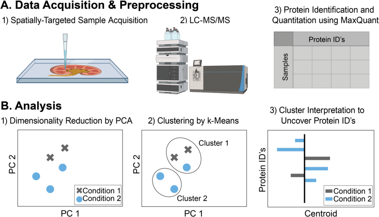
Pipeline for spatially targeted proteomics data acquisition and analysis. (A) Protein data were acquired from tissue samples using spatially targeted sample acquisition and then peptides were analyzed using LC-MS/MS. Data preprocessing involved protein identification and quantitation using MaxQuant software. (B) PCA was applied for dimensionality reduction and grouping of correlated and anticorrelated proteins among regions and time points. The PCA-processed data were clustered by k-means and cluster centers examined for protein identifications.

Data Analysis

We performed protein identification and quantitation using MaxQuant⁴⁰ as follows (Figure 1A). Raw LC-MS/MS files were processed using the label-free quantification method in MaxQuant version 1.6.7. Spectra were simultaneously searched against Mus musculus and S. aureus (strain USA300 LAC) reference databases downloaded from UniProt KB,⁵⁷ and the resultant peptide and subsequent protein identifications include the name of the species. These labeled identifications can later be used to separate the proteins by species. These were supplemented with the reversed sequences and common contaminants for quality control purposes. Acetyl (protein N-term) and oxidation (M) were set as variable modifications. Match between runs was not used and the LFQ min ratio count was set to 1. Minimal peptide length was seven amino acids. Peptide and protein false discovery rates (FDRs) were both set at 1%.

The resultant protein groups file containing label-free quantitation (LFQ) intensity values from MaxQuant, was used for the subsequent data analysis. In this file, each row contains the group of proteins that could be reconstructed from a set of peptides; proteins in each protein group are sorted based on the number of identified peptides in descending order. This protein groups file was analyzed for outliers using a z-score anomaly detection calculation. Briefly, z-scores were calculated based on the number of protein groups identified and samples with z-scores > |2| were excluded. Based on this calculation, 3 samples out of 42 total were excluded (Figures S1 and S2). Proteins identified as “reverse”, “only identified by site”, or “potential contaminants” were also removed, as well as proteins with fewer than two unique peptides identified. As a result of this filtering process and of the molecular heterogeneity between samples, there are many missing (LFQ) values in the data set. For the primary analysis in the paper, proteins with missing values in any of the samples were excluded from the subsequent data analysis, resulting in a data set comprising only 287 proteins (rather than the 3613 protein rows from the start). To also assess broader coverage, a secondary (inclusive) analysis was also conducted, where instead of removal, the missing values were zero-filled and analyzed using the same subsequent data analysis method. The latter results are reported in the Supporting Information.

Using Python version 3.7, we applied Scikit-learn’s principal component analysis with a randomized solver⁵⁸ to generate an array of 39 ranked components (the maximum, given that there are 39 samples). This array of PCA-transformed data (of size 39 × 39 instead of the original 39 × 287) was then used for k-means clustering using Scikit-learn’s KMeans implementation (Figure 1B and Figure 3D). A range of k values from 2 to 15 was tested using silhouette scores⁵⁹ as a performance metric⁵⁹ to determine the optimal k number of clusters. Upon determining the optimal k value to be 4 (Figure S3), the k-means clustering algorithm was deployed to assign cluster membership to each sample; aside from setting the random_state parameter to a fixed but randomly selected integer (42) to maintain reproducibility across runs, the default parameters were used. Cluster centroids for each cluster, which represent the average for all points belonging to the cluster, were used for biological interpretation with 10% of proteins (n = 29) with highest absolute values labeled (Figure 4 and Table S2). Since the k-means clustering was performed on PCA-transformed data, the resultant cluster centroids are in the form of 4 rows (one per cluster) and 39 columns (one for each principal component). To interpret the cluster centroids in terms of the protein groups, we cast the centroids back to the original measurement space by performing matrix multiplication between the centroid table (of size 4 × 39) and the PCA scores table (of size 39 × 287), thereby generating a final matrix of size 4 × 287 (Figure 1B). For the secondary (inclusive) analysis as a supplement to the original analysis, we also performed the PCA and k-means clustering on the full proteomic data set, zero-filling the missing values, which resulted in a total feature set of 3613 proteins. For this analysis, a k of 5 was selected and the resultant cluster centroids were extracted in the same way as described above, with the note that the final centroid matrix was in that case of size 5 × 3613 (Figures S4 and Figure S5 and Table S3).

Figure 3.

Principal component analysis and k-means clustering results of proteins of an S. aureus-infected murine kidney. (A) PCA was performed on protein LFQ intensity values acquired from 3 regions and 2 time points. This unsupervised approach separates the SAC and interface (left) from the cortex samples with no visible infection (right). (B) Samples also seem to cluster based on biological replicate within the PCA space. (C) There is a separation among the samples 4 and 10 days postinfection within samples acquired from region of infection; this separation is not seen from samples acquired from the cortex where there was no visible infection. (D) k-Means clustering was used to cluster the samples after PCA; k = 4 was determined using silhouette scores as a metric. To aid in interpretation, clusters are labeled by the regions and time points from which samples were collected.

Figure 4.

Molecular differentiators among regions of S. aureus-infected kidney. (A) All four cluster centers are overlaid with 10% of proteins (n = 29) with highest absolute values labeled. Underlined are the three proteins with overall highest absolute centroid values; * = proteins involved in the tricarboxylic acid cycle, ** = proteins involved in maintaining cell structure and facilitating tissue repair/remodeling.

The absolute centroid values were summed per cluster and the 100 and 175 proteins for the nonimputed and zero-imputed data sets, respectively, with highest accumulated centroid values were selected for gene ontology analysis. The original LFQ intensity values for those top proteins were extracted for each sample and their intensity was standardized per protein by removing the mean and scaling to unit variance. These standardized protein intensity values were averaged per cluster, and proteins with a standardized intensity greater than zero were selected for gene ontology enrichment analysis, which was performed using the protein analysis through evolutionary relationships (PANTHER) classification system (version 16.0) for each set of proteins per cluster.⁶⁰ Only murine proteins were used for the gene ontology analysis since PANTHER does not include the S. aureus strain USA300 LAC in their databases. The resultant protein classes were summarized (Figure 5, Figure S6, Table S4, and Table S5).

Figure 5.

Gene ontology analysis. Gene ontology analysis was performed using the 100 proteins with highest accumulated absolute centroid values. The LFQ intensity for these proteins were normalized across all samples and those with values above 0 were analyzed using the PANTHER classification system based on protein class. Panels A–D are sorted from no infection (cortex 4 DPI and 10 DPI) to most infection (interface 10 DPI and SAC 10 DPI). The total number of proteins in each cluster are as follows: (A) 31, (B) 28, (C) 47, and (D) 48. Panel E shows three protein classes with differences among regions of infection versus no infection, and the total number of proteins in each class.

Figures were generated using Matplotlib,⁶¹ circlize,⁶² and Numbers for iOS, except the schematic for Figure 1, Figure 2A, and the TOC graphic, which were created with BioRender.com. All code for data analysis can be found at https://github.com/kavyasharman/microlesa (Supporting Information 1 and Supporting Information 2).

Figure 2.

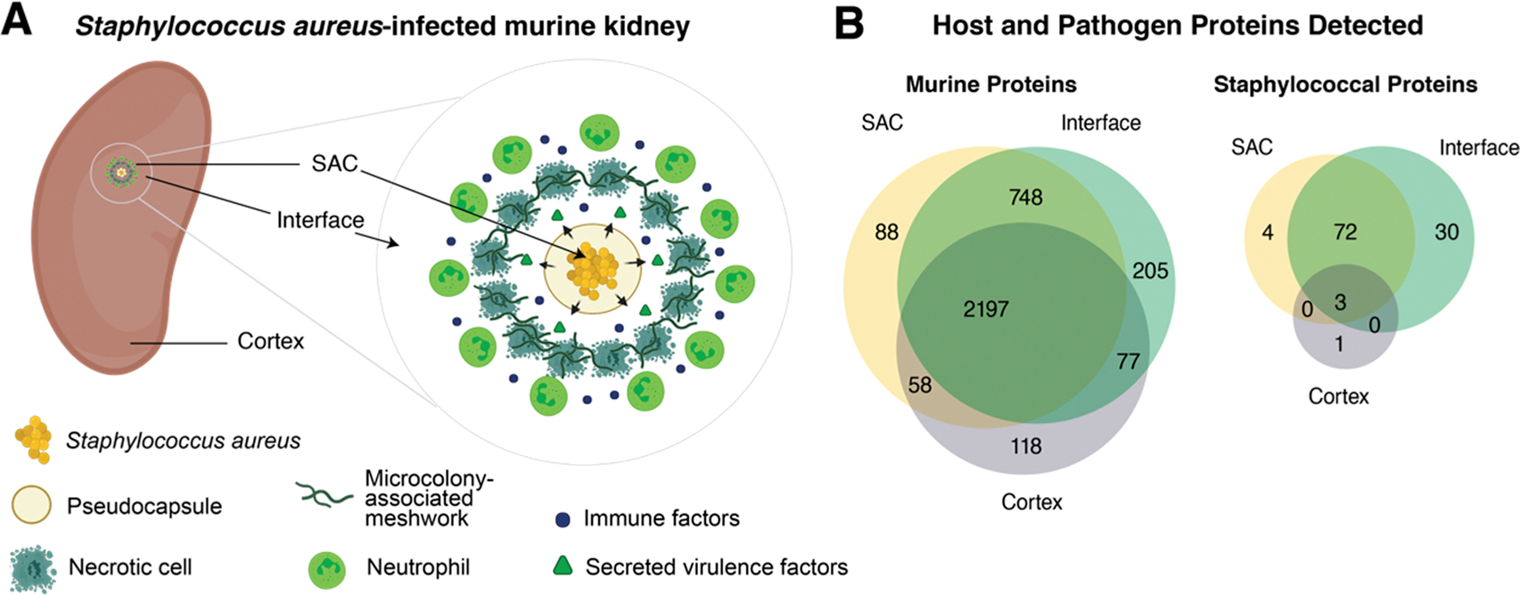
S. aureus-infected murine kidney. (A) Graphical depiction of the host–pathogen interface of S. aureus infection within a murine kidney. SAC: staphylococcal abscess community. (B) Summary of the total number of host and pathogen proteins detected.

RESULTS AND DISCUSSION

S. aureus is a Gram-positive pathogen that is known to cause skin and soft tissue infections.⁶³ A hallmark of S. aureus infection is the formation of soft-tissue abscesses. Development of these three-dimensional structures are accompanied by changes in architecture as well as cellular and molecular compositions of host tissue.^38,56,63,64 Understanding the formation of these structures, including the molecular changes across different regions of, and in proximity to, the abscess is particularly relevant to understand how S. aureus interacts with the host immune system and how staphylococcal infections progress.

In this original experiment,³⁸ mice were infected with fluorescently labeled strains of S. aureus and their kidneys were isolated for analysis with microLESA at 4 or 10 DPI (Figure 1). Three regions were selected for analysis:³⁸ the staphylococcal abscess community (SAC), the nonabscessed cortex, and the interface between the abscess and the surrounding nonabscessed cortex (Figure 2A). Of the 42 samples, 20 were measured at 4 DPI (5 from the interface, 7 from nonabscessed cortex, and 8 from the SAC) and 22 at 10 DPI (6 from the interface, 7 from nonabscessed cortex, and 9 from the SAC). There were 3 biological replicates for each DPI category, making for 6 mice total (3 mice at 4 DPI and 3 mice at 10 DPI). Multiple ROIs from each of the 3 regions were sampled for analysis.

Protein Identification and Quantitation

An average of 1500 proteins were detected from each sample. Proteins that were not identified within a sample but detected in another sample or that were below the limit of detection were not reported, generating a missing value. Missing values from each sample ranged from 31 to 77% (Table S1, Figure S1, and Figure S2). There are multiple options for handling missing values, including imputation or removing proteins not detected consistently across samples. For our primary (nonimputing) analysis, proteins with missing values in one or more samples were excluded, resulting in a remaining total of 287 proteins detected and quantified across all samples.

After protein identification and quantitation, the resultant protein groups containing LFQ intensity values were analyzed for outliers by calculating z-scores for each sample based on the number of protein groups identified in each and excluding samples with a z-score > |2|. From this preprocessing, we generated a table containing protein group versus LFQ intensity, consisting of 39 samples total representing 3 regions (SAC, interface, cortex), 2 time points (4 DPI, 10 DPI), and 287 total protein groups (cross section across all 39 samples). Of these proteins, all 287 were identified as murine using the MaxQuant database search as explained above (Figure 2B). It is important to note that although in this paper and case study MaxQuant LFQ was used as the input data, other value types such as iBAQ intensities or raw ion intensities can also be provided as input data for this PCA + k-means workflow, without it requiring substantial changes. The choice of which input type to supply depends on what is most appropriate for the data set and analysis at hand.

Next, we sought to develop an unsupervised multivariate method that would allow us to capture the unique proteomic signature from each of the distinct ROIs, but without focusing on a specific protein species and instead providing broad coverage across a panel of proteins. The entire data set of protein group measurements, excluding those with missing values, for each of the protein groups (n = 287) was used for the analysis and each sample was annotated by time point (4 DPI (n = 20) and 10 DPI (n = 19)) and region (SAC (n = 17), interface (n = 11), or cortex (n = 11)). The data were not pooled by technical or biological replicates in order to provide as many measurements as possible for the unsupervised learning and to avoid an “averaging out” of information, which could underpower the analysis given the already low number of samples (n = 39).

Principal Component Analysis Followed by k-Means Clustering

The first part of our analytical process consists of PCA to address the “curse of dimensionality”, which broadly summarizes the myriad challenges in analyzing and identifying patterns in high-dimensional data. PCA groups correlating and anticorrelating features into a series of orthogonal components. In doing so, the data are transformed from a high-dimensional space into a lower-dimensional space while attempting to minimize the loss of information.

PCA with a randomized solver⁵⁸ was applied to reduce the dimensionality of the complete data set and group correlated/anticorrelated samples based on the protein LFQ intensity values. In doing so, the dimensions of the data set were reduced, from a matrix of dimensions [39 × 287] to that of [39 × 39]. All components were retained to avoid information loss. We found that the first and second principal components accounted for 81.35 and 10.61% of the explained variance, respectively, and together, these components separated the data by region and time point (Figure 3A). We further labeled the data by regions and time points to explore variation present among these subsets (Figure 3A,C). In terms of region (Figure 3A), samples collected from the (uninfected) cortex cluster seem to separate away (to the right in the figure) from those collected from the interface and SAC, suggesting similarity between the interface and SAC proteomics, which is expected since both contain regions of infection. There is also a degree of protein similarity among the biological replicates because samples within the PCA seem to cluster similarly based on biological replicate (Figure 3B).

Examining the PCA results as a function of time points reveals a clear distinction between samples collected 4 and 10 DPI (Figure 3C), suggesting that infection time is a key differentiator among the protein patterns in both interface and SAC regions. Some interface samples that were collected 10 DPI overlap closely with SAC samples collected 10 DPI, suggesting that, after 10 DPI, the interface proteome could potentially start resembling that of the SAC. This observation is indicative of interface heterogeneity and a differential impact of infection among regions of tissue surrounding bacterial abscesses. It may also imply spatial expansion of the immune response and expanding tissue damage as result of the progressing infection, but this would require subsequent follow-up study and validation. Conversely, samples acquired from the cortex where there was no infection visibly present do not show a separation between 4 and 10 DPI.

While PCA tends to group the data based on the protein (LFQ) content of each sample, a secondary step is required to identify and interpret protein patterns. We hypothesized that an automated unsupervised clustering method could provide further insight into the spatial patterns of staphylococcal infection over early and late time points. Clustering is a common approach for interpreting high-dimensional data and works by grouping similar samples together based on variation among measured features. Within a protein data set, samples that contain similar protein expression patterns can be grouped and the underlying variation among the groups can potentially represent biologically relevant information. Of the myriad methods for clustering,^65–67 k-means clustering^68–70 (with a Euclidean distance metric) was chosen because the cluster centroids that represent the average protein pattern for each group can provide rapid and straightforward protein-level insight.

We applied k-means clustering to the PCA-transformed data. Silhouette scores⁵⁹ were used as a performance metric (Figure S3); 3, 4, and 5 were relatively equally good choices so a k of 4 was chosen as it lies at the center of this equally good range. Each sample was then assigned membership to one of four clusters (Figure 3D). Descriptors of samples in each cluster were added to the figure to aid in interpretation (Figure 3D).

Samples from the nonabscessed cortex regions are grouped into cluster 3, comprising samples from both 4 and 10 DPI. However, the k-means clustering led to varied cluster membership for the samples extracted from areas of infection. For instance, cluster 4 consists of samples collected from the cortex and interface 4 DPI and 10 DPI, suggesting that the proteome of the interface early in the infection is more like the cortex than the proteome of other interface samples or the SAC. Cluster 2 consists of interface samples 4 and 10 DPI as well as SAC samples 4 and 10 DPI. Cluster 1 only consists of samples 10 DPI from both interface and SAC. The clustering patterns of interface and SAC samples reveal two interesting observations. First, that the SAC samples can be categorized into two different clusters is consistent with findings of previously observed abscess heterogeneity^38,56 and indicates that there can still be changes in abscesses that are seemingly fully formed. Second, abscess formation and mounting immune response may take up to 10 DPI to manifest proteomic changes in the interface even though abscesses can be seen at the 4 DPI mark. The distinction in the proteome between the early and late interface is especially evident as interface samples are seen clustering with cortex and SAC samples at varying time points. In summary, these observations from the k-means clustering analysis reveal patterns of staphylococcal infection progression and heterogeneity in the proteome among specific regions of infection.

Cluster Interpretation

Our multivariate analysis provides broad proteomic insight based on underlying proteomic (LFQ) variations. The method provides a high-level understanding into protein differences between time points and regions within an S. aureus infection model. To identify a subset of relevant proteins from the 287 total measured proteins used for this analysis, we interpreted the average centroids of each cluster. Using PCA followed by k-means clustering, we can automatically rank proteins that significantly contribute to the clustering model; proteins with high absolute centroid values contribute more as differentiators to the clustering model than those with low absolute centroid values, and therefore are more likely to reveal biological insight. Average centroids for each of the four clusters were extracted, with 287 proteins or protein groups as observations and absolute cluster centroid values as variables. All proteins are represented in each centroid and the centroid value for each protein indicates the degree to which that protein is relevant to that cluster. Proteins with high absolute values are more relevant to a given cluster than those with low values.

Of the 287 proteins analyzed, the top 10% with highest absolute centroid values were labeled for interpretation (Figure 4). α-Globin 1, cytoplasmic actin, and β-globin have the highest absolute centroid values and distinguish clusters comprising samples from infected regions (interface and SAC) versus those from the cortex. Among the 29 highest ranked proteins are mitochondrial ATP synthase subunits α and β and pyruvate kinase, which are involved in the tricarboxylic acid cycle. We also note proteins involved in maintaining cell structure and facilitating tissue repair/remodeling such as myosin-9, cytoplasmic actin, filamin, and fibrinogen.

Given the low number of samples (n = 39) encompassing multiple time points and regions, eliminating proteins with missing values in one or more samples resulted in eliminating a substantial amount of measured protein data. As a comparison, we reanalyzed the data, this time using all the proteomics data with an imputation approach to handle the missing values. Imputation has been systematically evaluated and successfully implemented for mass spectrometry data sets and studies in the past.^50,58,71 A recent study found that techniques such as local least-squares, random forest, and Bayesian PCA missing value estimation worked well for label-free data-independent acquisition mass spectrometry (DIA-MS) data sets.⁵¹ However, this study among others has shown that for an imputation to be helpful in the final analysis, it must model actual observed phenomena. For the case of microLESA data where proteins are sampled from small, biologically heterogeneous regions of tissue, the probability that a protein was not detected when its value is missing is higher than if we were to impute a value based on an imputation method. Therefore, for this analysis, we chose a simple model with the assumption that if a protein was not measured, it was below the limit of detection or not present in the sample. As such, missing values were zero-filled. This type of imputation is a common approach for handling missing value, as opposed to our primary approach, where columns with missing values were removed such that only globally present proteins are used for the analysis.^50,51,71

Upon analyzing the data set with zero-filled values, comprising 3,613 proteins in total, we found that the PCA and k-means clustering results remained largely the same (Figure S4). The key differences are in the PCA explained variance (components 1 and 2 now respectively represent 77.26 and 10.3% of the data as compared to the 81.35 and 10.61% previously, Figure S4A–C), the number of k clusters (silhouette score analysis revealed a k of 5 to be optimal for this larger richer data set with imputed values, Figure S4D), and resultant cluster membership of samples. When analyzing the zero-filled larger proteomics data set, there is a new cluster intermediately situated between the cortex and interface/SAC 4 and 10 DPI clusters. This new cluster comprises samples from the cortex 4 and 10 DPI as well as interface 4 DPI. Samples that were originally organized into a single cluster comprising cortex 4 and 10 DPI split into two clusters, with two samples acquired from the cortex at 4 DPI comprising one cluster and six samples acquired from the cortex at 4 and 10 DPI comprising a second cluster. This indicates that with the inclusion of all proteins and zero-filling those with missing values, we can observe more perceived separation among the samples. The cluster with interface and SAC samples 10 DPI remains unchanged.

In analyzing the cluster centroids, we found that cluster membership is largely driven by the same proteins, such as α-globin 1, cytoplasmic actin, and β-globin (Figure S5). However, notably present in this list are several immune-response related factors such as S100-A9 and prothymosin α.⁷² Although the primary drivers of cluster membership remained the same, the same analytical process applied to the larger imputed data set provided a broader description of the host–pathogen interface, uncovering additional target proteins that can be further validated.

It is important to note that interpreting the PCA pseudoprotein signature must be done carefully because it represents combinations of protein LFQ data that capture as much of the observed variance as possible. For example, the PCA result might be be skewed by high-intensity values for proteins that may not be biologically relevant, or miss low-intensity valued proteins that nevertheless may hold biological significance, but whose importance is mathematically hard to discern in the presence of proteins with higher intensity values. Although the MaxQuant software performs normalization across the entire sample set during the LFQ intensity calculation, differences in overall protein intensity values may still affect the final output. This relays a fundamental concern in proteomics, which is the extremes in dynamic range of signal and biological abundance for detected proteins.

PCA is also vulnerable to proteins that may describe non-Gaussian distributions in the LFQ intensity domain, going against a key assumption for PCA.⁶⁷ As such, we refrain from attempting to overinterpret the pseudoprotein signatures, and limit ourselves to exploring in each cluster only the highest absolute centroid values. In doing so, we only claim to find a focused subset of interesting proteins that merit further investigation, from among the hundreds that were measured over the entire experiment, thereby providing a means of efficiently identifying candidates for future investigation. Similarly, alternative clustering methods such as hierarchical clustering can also be used to analyze the dimensionality reduced proteomics data. In this study, k-means was selected due to the ease of interpretation of the cluster centroids, which represent the average protein pattern for each cluster. In summary, this unsupervised multivariate method provides a way to efficiently analyze highly complex spatially targeted proteomics data and provide an effective way of highlighting a panel of potential drivers of biological differences among regions of interest.

Gene Ontology Analysis

While identifying individual proteins from thousands measured is an important output of this biocomputational process, understanding the functional categories of each protein can provide additional biological insight. We used the PANTHER classification system⁶⁰ to perform a gene ontology analysis of the proteins driving the clustering algorithm. The absolute centroid values were summed across all four clusters, and the top 100 and 175 proteins for the nonimputed and zero-imputed data sets, respectively, with highest accumulated centroid values selected for gene ontology analysis. For a broader or more narrow biological interpretation, more or fewer proteins can be selected at this stage of the analysis. Original LFQ intensity values for the selected proteins were retrieved, and their LFQ intensity was standardized per protein by removing the mean and scaling to unit variance. The standardized protein intensity values were averaged per cluster and proteins with positive values per cluster were extracted. These proteins per cluster were analyzed using PANTHER for a gene ontology analysis, and the resultant protein classes found in each cluster were determined (Figures 5 and S5).

Results indicate that the proteins driving the clustering model comprise 13 protein classes, including cytoskeletal and metabolic processes (Figure 5). Panels A–D are sorted from regions distant from the abscess with no visible bacteria present (cortex 4 DPI and 10 DPI) to those in proximity to abscesses at the later time point (interface/SAC 10 DPI), and panel E shows three protein classes (cytoskeletal, metabolite interconversion enzyme, and calcium binding) with distinct changes between regions of infection (interface/SAC) and no infection (cortex/early interface).

Our study identified cytoskeletal proteins that are enriched at the site of infection (abscess and interface), particularly at the later time point. These findings are indicative of extensive tissue damage resulting from S. aureus residing and proliferating within the tissue, as well as subsequent repair and remodeling efforts by the host.⁷³ Additionally, we detected an enrichment of established immune factors, such as calcium-binding proteins, comprising different Annexins, which have been recently implicated in the defense against Gram-positive infections.^74–76 Specifically, Annexins A2 and A3 were increased in two clusters: (i) interface 4 DPI and 10 DPI, SAC 4 DPI and 10 DPI, and (ii) interface 10 DPI, SAC 10 DPI. Further, Annexin A5 showed increased abundance in the Interface 10 DPI, SAC 10 DPI cluster. Recent studies suggest that Annexin A2 interacts with staphylococcal clumping factors A and B, facilitating attachment to epithelial cells.^75,76 Another study concluded that binding of Annexin A2 allows S. aureus to anchor onto vascular endothelial cells, establishing this host protein as an important factor for initiating staphylococcal interaction with its host.⁷⁷ In contrast, little is known about the roles of Annexins A3 and A5 during infection with S. aureus. A transcriptomics study revealed that Annexin A3 expression is restricted to neutrophils and is increased in the blood of patients with sepsis.⁷⁸ Annexin A5, which was increased in the Interface 10 DPI, SAC 10 DPI cluster, has been shown to aid survival in a murine sepsis model by inhibiting HMGB1-mediated proinflammation and coagulation.⁷⁹ Despite these findings, it is not clear how Annexins A3 and A5 affect the host–pathogen interplay, particularly in the context of S. aureus soft-tissue infections. While our study relies on a relatively small sample size, our data clearly show that Annexins A2, A3, and A5 are highly abundant at the site of infection. The data presented here and previous studies on Annexins allow us to speculate that while A2 may be facilitating staphylococcal anchoring in the tissue, A3 and A5 may confer varying degrees of host protection during staphylococcal infection.

We also performed a gene ontology analysis using the larger, zero-filled data set (Figure S6). As with the centroid analysis above, the protein classes remained largely the same, with the addition of defense/immunity proteins present in clusters with infected samples as well as additional calcium-binding proteins such as the major immune component calprotectin.

This systems-level summary of a complex biological model demonstrates the utility of the data generated through our method and presents the potential for future biology-driven investigation and experimentation. The gene ontology analysis demonstrated here is one of many potential interpretations of the cluster centers. Another way of interpreting the cluster centroids can include building protein–protein interaction networks using proteins with high accumulated absolute centroid values as seeds. We also acknowledge that the samples chosen in this study belonged to biologically distinct locations with profound protein changes. While we cannot directly speak to the performance of this method on a different data set with more nuanced protein heterogeneity, there are multiple opportunities to tune the pipeline to be more robust or sensitive to the protein changes within the study. There would need to be some prior knowledge about the source of protein variation, but those changes could be used to inform the PCA, the number of k-means clusters, and the approach to cluster interpretation.

Though this method was applied to spatially targeted proteomics data acquired by microLESA, it can be extended to multiomics data involving metabolites, lipids, and peptides acquired using other spatially targeted approaches such as liquid extraction surface analysis,^34,36,80 liquid microjunction,^81,82 nanoPOTS,^29–31 tissue punch biopsies,^83,84 laser capture microdissection,^42–45,85 and hydrogel extractions.^86–88

CONCLUSION

We have developed a rapid automated unsupervised method for analyzing high-dimensional spatially targeted proteomics data utilizing PCA followed by k-means clustering. Here, we applied this multivariate analysis to study S. aureus infection in murine kidney. The k-means clustering results revealed molecular heterogeneity in the abscesses and the interface region between areas of infection and noninfection that goes beyond what can be seen by microscopy alone. Proteins that were driving the clustering algorithm, and thereby likely to play a role in staphylococcal infection, were extracted from cluster centroids; these were found to be involved in key metabolic processes and cytoskeletal reorganization. The subsequent gene ontology analysis of proteins with high accumulated absolute centroid values revealed that proteins involved in calcium-dependent, metabolite interconversion, and cytoskeletal processes were enriched in sites of infection, especially at the 10 DPI time point. Collectively, we identified both key proteins and processes that are enriched at the site of staphylococcal infection. These findings demonstrate that this multivariate approach is a powerful method that provides a means of rapidly filtering complex biological data to determine the most relevant species from hundreds to thousands of measured proteins in the form of ranked protein lists and pathway enrichments, thereby providing a systems-level view into complex molecular biological processes.

REFERENCES

- (1).Aebersold R; Mann M Mass spectrometry-based proteomics. Nature 2003, 422, 198–207. [DOI] [PubMed] [Google Scholar]
- (2).Bantscheff M; Schirle M; Sweetman G; Rick J; Kuster B Quantitative mass spectrometry in proteomics: a critical review. Anal. Bioanal. Chem. 2007, 389, 1017–1031. [DOI] [PubMed] [Google Scholar]
- (3).Han X; Aslanian A; Yates JR 3rd Mass spectrometry for proteomics. Curr. Opin. Chem. Biol. 2008, 12, 483–490. [DOI] [PMC free article] [PubMed] [Google Scholar]
- (4).Yates JR; Ruse CI; Nakorchevsky A Proteomics by Mass Spectrometry: Approaches, Advances, and Applications. Annu. Rev. Biomed. Eng. 2009, 11, 49–79. [DOI] [PubMed] [Google Scholar]
- (5).Baker ES; et al. Mass spectrometry for translational proteomics: progress and clinical implications. Genome Med. 2012, 4, 63. [DOI] [PMC free article] [PubMed] [Google Scholar]
- (6).Noor Z; Ahn SB; Baker MS; Ranganathan S; Mohamedali A Mass spectrometry-based protein identification in proteomics- A review. Briefings in Bioinformatics 2021, 22, 1620–1638. [DOI] [PubMed] [Google Scholar]
- (7).Pitt JJ Principles and applications of liquid chromatography-mass spectrometry in clinical biochemistry. Clin. Biochem. Rev. 2009, 30, 19–34. [PMC free article] [PubMed] [Google Scholar]
- (8).Chen G; Pramanik BN Application of LC/MS to proteomics studies: current status and future prospects. Drug Discovery Today 2009, 14, 465–471. [DOI] [PubMed] [Google Scholar]
- (9).Srinivas PR; Verma M; Zhao Y; Srivastava S Proteomics for Cancer Biomarker Discovery. Clin. Chem. 2002, 48, 1160–1169. [PubMed] [Google Scholar]
- (10).Sallam RM Proteomics in Cancer Biomarkers Discovery: Challenges and Applications. Dis. Markers 2015, 2015, 321370. [DOI] [PMC free article] [PubMed] [Google Scholar]
- (11).Shruthi BS; Vinodhkumar P; Selvamani. Proteomics: A new perspective for cancer. Adv. Biomed. Res. 2016, 5, 67. [DOI] [PMC free article] [PubMed] [Google Scholar]
- (12).Scott EM; Carter AM; Findlay JBC The application of proteomics to diabetes. Diabetes Vasc. Dis. Res. 2005, 2, 54–60. [DOI] [PubMed] [Google Scholar]
- (13).Bhat S; Jagadeeshaprasad MG; Venkatasubramani V; Kulkarni MJ Abundance matters: role of albumin in diabetes, a proteomics perspective. Expert Rev. Proteomics 2017, 14, 677–689. [DOI] [PubMed] [Google Scholar]
- (14).Wang N; Zhu F; Chen L; Chen K Proteomics, metabolomics and metagenomics for type 2 diabetes and its complications. Life Sci. 2018, 212, 194–202. [DOI] [PubMed] [Google Scholar]
- (15).Fu J; et al. Advances in Current Diabetes Proteomics: From the Perspectives of Label- free Quantification and Biomarker Selection. Curr. Drug Targets 2019, 21, 34–54. [DOI] [PubMed] [Google Scholar]
- (16).Van Eyk JE Proteomics: unraveling the complexity of heart disease and striving to change cardiology. Curr. Opin. Mol. Ther. 2001, 3, 546–553. [PubMed] [Google Scholar]
- (17).McGregor E; Dunn MJ Proteomics of the heart: unraveling disease. Circ. Res. 2006, 98, 309–321. [DOI] [PubMed] [Google Scholar]
- (18).Fu Q; Van Eyk JE Proteomics and heart disease: identifying biomarkers of clinical utility. Expert Rev. Proteomics 2006, 3, 237–249. [DOI] [PubMed] [Google Scholar]
- (19).Baetta R; Pontremoli M; Martinez Fernandez A; Spickett CM; Banfi C Proteomics in cardiovascular diseases: Unveiling sex and gender differences in the era of precision medicine. J. Proteomics 2018, 173, 62–76. [DOI] [PubMed] [Google Scholar]
- (20).Caprioli RM; Farmer TB; Gile J Molecular Imaging of Biological Samples: Localization of Peptides and Proteins Using MALDI-TOF MS. Anal. Chem. 1997, 69, 4751–4760. [DOI] [PubMed] [Google Scholar]
- (21).Stoeckli M; Chaurand P; Hallahan DE; Caprioli RM Imaging mass spectrometry: a new technology for the analysis of protein expression in mammalian tissues. Nat. Med. 2001, 7, 493–496. [DOI] [PubMed] [Google Scholar]
- (22).Amstalden van Hove ER; Smith DF; Heeren RMA A concise review of mass spectrometry imaging. J. Chromatogr. A 2010, 1217, 3946–3954. [DOI] [PubMed] [Google Scholar]
- (23).McDonnell LA; Heeren RMA Imaging mass spectrometry. Mass Spectrom. Rev. 2007, 26, 606–643. [DOI] [PubMed] [Google Scholar]
- (24).Norris JL; Caprioli RM Analysis of tissue specimens by matrix-assisted laser desorption/ionization imaging mass spectrometry in biological and clinical research. Chem. Rev. 2013, 113, 2309–2342. [DOI] [PMC free article] [PubMed] [Google Scholar]
- (25).Burnum KE; Frappier SL; Caprioli RM Matrix-assisted laser desorption/ionization imaging mass spectrometry for the investigation of proteins and peptides. Annu. Rev. Anal. Chem. (Palo Alto. Calif) 2008, 1, 689–705. [DOI] [PubMed] [Google Scholar]
- (26).Spraggins JM; et al. Next-generation technologies for spatial proteomics: Integrating ultra-high speed MALDI-TOF and high mass resolution MALDI FTICR imaging mass spectrometry for protein analysis. Proteomics 2016, 16, 1678–1689. [DOI] [PMC free article] [PubMed] [Google Scholar]
- (27).Aichler M; Walch A MALDI Imaging mass spectrometry: current frontiers and perspectives in pathology research and practice. Lab. Investig. 2015, 95, 422–431. [DOI] [PubMed] [Google Scholar]
- (28).Ryan DJ; Spraggins JM; Caprioli RM Protein identification strategies in MALDI imaging mass spectrometry: a brief review. Curr. Opin. Chem. Biol. 2019, 48, 64–72. [DOI] [PMC free article] [PubMed] [Google Scholar]
- (29).Zhu Y; et al. Spatially Resolved Proteome Mapping of Laser Capture Microdissected Tissue with Automated Sample Transfer to Nanodroplets*. Mol. Cell. Proteomics 2018, 17, 1864–1874. [DOI] [PMC free article] [PubMed] [Google Scholar]
- (30).Zhu Y; Piehowski PD; Zhao R; Chen J; Shen Y; Moore RJ; Shukla AK; Petyuk VA; Campbell-Thompson M; Mathews CE; Smith RD; Qian W-J; Kelly RT Nanodroplet processing platform for deep and quantitative proteome profiling of 10–100 mammalian cells. Nat. Commun. 2018, 9 (1), 882. [DOI] [PMC free article] [PubMed] [Google Scholar]
- (31).Piehowski PD; Zhu Y; Bramer LM; Stratton KG; Zhao R; Orton DJ; Moore RJ; Yuan J; Mitchell HD; Gao Y; Webb-Robertson B-JM; Dey SK; Kelly RT; Burnum-Johnson KE Automated mass spectrometry imaging of over 2000 proteins from tissue sections at 100-μm spatial resolution. Nat. Commun. 2020, 11, 8. [DOI] [PMC free article] [PubMed] [Google Scholar]
- (32).Kelly R; et al. Single Cell Proteome Mapping of Tissue Heterogeneity Using Microfluidic Nanodroplet Sample Processing and Ultrasensitive LC-MS. J. Biomol. Technol. 2019, 30, S61. [Google Scholar]
- (33).Williams SM; et al. Automated Coupling of Nanodroplet Sample Preparation with Liquid Chromatography-Mass Spectrometry for High-Throughput Single-Cell Proteomics. Anal. Chem. 2020, 92, 10588–10596. [DOI] [PMC free article] [PubMed] [Google Scholar]
- (34).Sarsby J; et al. Liquid Extraction Surface Analysis Mass Spectrometry Coupled with Field Asymmetric Waveform Ion Mobility Spectrometry for Analysis of Intact Proteins from Biological Substrates. Anal. Chem. 2015, 87, 6794–6800. [DOI] [PubMed] [Google Scholar]
- (35).Schey KL; Anderson DM; Rose KL Spatially-directed protein identification from tissue sections by top-down LC-MS/MS with electron transfer dissociation. Anal. Chem. 2013, 85, 6767–6774. [DOI] [PMC free article] [PubMed] [Google Scholar]
- (36).Wisztorski M; et al. Droplet-based liquid extraction for spatially-resolved microproteomics analysis of tissue sections. Methods in Molecular Biology; Humana Press Inc., 2017; Vol. 1618, pp 49–63. [DOI] [PubMed] [Google Scholar]
- (37).Ryan DJ; et al. MicroLESA: Integrating Autofluorescence Microscopy, in Situ Micro-Digestions, and Liquid Extraction Surface Analysis for High Spatial Resolution Targeted Proteomic Studies. Anal. Chem. 2019, 91, 7578–7585. [DOI] [PMC free article] [PubMed] [Google Scholar]
- (38).Guiberson ER; et al. Spatially Targeted Proteomics of the Host-Pathogen Interface during Staphylococcal Abscess Formation. ACS Infect. Dis. 2021, 7, 101–113. [DOI] [PMC free article] [PubMed] [Google Scholar]
- (39).Cox J; Mann M MaxQuant enables high peptide identification rates, individualized p.p.b.-range mass accuracies and proteome-wide protein quantification. Nat. Biotechnol. 2008, 26, 1367–1372. [DOI] [PubMed] [Google Scholar]
- (40).Tyanova S; Temu T; Cox J The MaxQuant computational platform for mass spectrometry-based shotgun proteomics. Nat. Protoc. 2016, 11, 2301–2319. [DOI] [PubMed] [Google Scholar]
- (41).Piehowski PD; Zhu Y; Bramer LM; Stratton KG; Zhao R; Orton DJ; Moore RJ; Yuan J; Mitchell HD; Gao Y; Webb-Robertson B-JM; Dey SK; Kelly RT; Burnum-Johnson KE Automated mass spectrometry imaging of over 2000 proteins from tissue sections at 100-μm spatial resolution. Nat. Commun. 2020, 11, 8. [DOI] [PMC free article] [PubMed] [Google Scholar]
- (42).Satoskar AA; et al. Characterization of Glomerular Diseases Using Proteomic Analysis of Laser Capture Microdissected Glomeruli. Mod. Pathol 2012, 25, 709–721. [DOI] [PMC free article] [PubMed] [Google Scholar]
- (43).Cazares LH; et al. Normal, benign, preneoplastic, and malignant prostate cells have distinct protein expression profiles resolved by Surface Enhanced Laser Desorption/Ionization mass spectrometry. Clin. Cancer Res. 2002, 8, 2541–2552. [PubMed] [Google Scholar]
- (44).Datta S; et al. Laser capture microdissection: Big data from small samples. Histol. Histopathol. 2015, 30, 1255–1269. [DOI] [PMC free article] [PubMed] [Google Scholar]
- (45).Schuetz CS; et al. Progression-specific genes identified by expression profiling of matched ductal carcinomas in situ and invasive breast tumors, combining laser capture microdissection and oligonucleotide microarray analysis. Cancer Res. 2006, 66, 5278–5286. [DOI] [PubMed] [Google Scholar]
- (46).Alevizos I; et al. Oral cancer in vivo gene expression profiling assisted by laser capture microdissection and microarray analysis. Oncogene 2001, 20, 6196–6204. [DOI] [PubMed] [Google Scholar]
- (47).Kunz GM; Chan DW The use of laser capture microscopy in proteomics research - A review. Dis. Markers 2004, 20, 155–160. [DOI] [PMC free article] [PubMed] [Google Scholar]
- (48).Shapiro JP; et al. A quantitative proteomic workflow for characterization of frozen clinical biopsies: Laser capture microdissection coupled with label-free mass spectrometry. J. Proteomics 2012, 77, 433–440. [DOI] [PMC free article] [PubMed] [Google Scholar]
- (49).Elias J; Heuschmann PU; Schmitt C; Eckhardt F; Boehm H; Maier S; Kolb-Maurer A; Riedmiller H; Mullges W; Weisser C; Wunder C; Frosch M; Vogel U Prevalence dependent calibration of a predictive model for nasal carriage of methicillin-resistant Staphylococcus aureus. BMC Infect. Dis. 2013, 13, 111. [DOI] [PMC free article] [PubMed] [Google Scholar]
- (50).Wei R; Wang J; Su M; Jia E; Chen S; Chen T; Ni Y Missing Value Imputation Approach for Mass Spectrometry-based Metabolomics Data. Sci. Rep. 2018, 8, 663. [DOI] [PMC free article] [PubMed] [Google Scholar]
- (51).Dabke K; Kreimer S; Jones MR; Parker SJ A simple optimization workflow to enable precise and accurate imputation of missing values in proteomic datasets. J. Proteome Res. 2021, 20, 3214–3229. [DOI] [PubMed] [Google Scholar]
- (52).Lazar C; Gatto L; Ferro M; Bruley C; Burger T Accounting for the Multiple Natures of Missing Values in Label-Free Quantitative Proteomics Data Sets to Compare Imputation Strategies. J. Proteome Res. 2016, 15, 1116–1125. [DOI] [PubMed] [Google Scholar]
- (53).Anderson DC; Li W; Payan DG; Noble WS A new algorithm for the evaluation of shotgun peptide sequencing in proteomics: Support vector machine classification of peptide MS/MS spectra and SEQUEST scores. J. Proteome Res. 2003, 2, 137–146. [DOI] [PubMed] [Google Scholar]
- (54).Klein O; Kanter F; Kulbe H; Jank P; Denkert C; Nebrich G; Schmitt WD; Wu Z; Kunze CA; Sehouli J; Darb-Esfahani S; Braicu I; Lellmann J; Thiele H; Taube ET MALDI-Imaging for Classification of Epithelial Ovarian Cancer Histotypes from a Tissue Microarray Using Machine Learning Methods. Proteomics - Clin. Appl. 2019, 13, 1700181. [DOI] [PubMed] [Google Scholar]
- (55).Swan AL; Mobasheri A; Allaway D; Liddell S; Bacardit J Application of Machine Learning to Proteomics Data: Classification and Biomarker Identification in Postgenomics Biology. Omi. A J. Integr. Biol. 2013, 17, 595–610. [DOI] [PMC free article] [PubMed] [Google Scholar]
- (56).Cassat JE; et al. Integrated molecular imaging reveals tissue heterogeneity driving host-pathogen interactions. Sci. Transl. Med. 2018, 10, 6361. [DOI] [PMC free article] [PubMed] [Google Scholar]
- (57).The UniProt Consortium; et al. UniProt: the universal protein knowledgebase in 2021. Nucleic Acids Res. 2021, 49, D480–D489. [DOI] [PMC free article] [PubMed] [Google Scholar]
- (58).Halko N; Martinsson PG; Tropp JA Finding structure with randomness: Probabilistic algorithms for constructing approximate matrix decompositions. SIAM Rev. 2011, 53, 217–288. [Google Scholar]
- (59).Rousseeuw PJ Silhouettes: A graphical aid to the interpretation and validation of cluster analysis. J. Comput. Appl. Math. 1987, 20, 53–65. [Google Scholar]
- (60).Mi H; et al. PANTHER version 16: a revised family classification, tree-based classification tool, enhancer regions and extensive API. Nucleic Acids Res. 2021, 49, D394–D403. [DOI] [PMC free article] [PubMed] [Google Scholar]
- (61).Hunter JD Matplotlib: A 2D graphics environment. Comput. Sci. Eng. 2007, 9, 90–95. [Google Scholar]
- (62).Gu Z; Gu L; Eils R; Schlesner M; Brors B Circlize implements and enhances circular visualization in R. Bioinformatics 2014, 30, 2811–2812. [DOI] [PubMed] [Google Scholar]
- (63).Cheng AG; DeDent AC; Schneewind O; Missiakas D A play in four acts: Staphylococcus aureus abscess formation. Trends in Microbiology 2011, 19, 225–232. [DOI] [PMC free article] [PubMed] [Google Scholar]
- (64).Casadevall A; Pirofski LA Host-pathogen interactions: Basic concepts of microbial commensalism, colonization, infection, and disease. Infect. Immun. 2000, 68, 6511–6518. [DOI] [PMC free article] [PubMed] [Google Scholar]
- (65).Hastie T; Tibshirani R; Friedman JH The Elements of Statistical Learning Data Mining, Inference, and Prediction; Springer Series in Statistics; Springer, 2009. [Google Scholar]
- (66).Sinitcyn P; Rudolph JD; Cox J Computational Methods for Understanding Mass Spectrometry–Based Shotgun Proteomics Data. Annu. Rev. Biomed. Data Sci. 2018, 1, 207–234. [Google Scholar]
- (67).Verbeeck N; Caprioli RM; Van de Plas R Unsupervised machine learning for exploratory data analysis in imaging mass spectrometry. Mass Spectrom. Rev. 2020, 39, 245–291. [DOI] [PMC free article] [PubMed] [Google Scholar]
- (68).Hartigan JA; Wong MA Algorithm AS 136: A K-Means Clustering Algorithm. Appl. Stat. 1979, 28, 100. [Google Scholar]
- (69).Lloyd SP Least Squares Quantization in PCM. IEEE Trans. Inf. Theory 1982, 28, 129–137. [Google Scholar]
- (70).MacQueen J Some methods for classification and analysis of multivariate observations. Proceedings of the Fifth Berkeley Symposium on Mathematical Statistics and Probability; The Regents of the University of California, 1967; Vol. 1, pp 281–296. [Google Scholar]
- (71).Karpievitch Y; et al. A statistical framework for protein quantitation in bottom-up MS-based proteomics. Bioinformatics 2009, 25, 2028–2034. [DOI] [PMC free article] [PubMed] [Google Scholar]
- (72).Santamaria-Kisiel L; Rintala-Dempsey AC; Shaw GS Calcium-dependent and -independent interactions of the S100 protein family. Biochem. J. 2006, 396, 201–214. [DOI] [PMC free article] [PubMed] [Google Scholar]
- (73).Ziesemer S; et al. Staphylococcus aureus α-Toxin Induces Actin Filament Remodeling in Human Airway Epithelial Model Cells. Am. J. Respir. Cell Mol. Biol. 2018, 58, 482–491. [DOI] [PubMed] [Google Scholar]
- (74).Gotoh M; et al. Annexins I and IV inhibit Staphylococcus aureus attachment to human macrophages. Immunol. Lett. 2005, 98, 297–302. [DOI] [PubMed] [Google Scholar]
- (75).Ashraf S; Cheng J; Zhao X Clumping factor A of Staphylococcus aureus interacts with AnnexinA2 on mammary epithelial cells. Sci. Rep. 2017, 7, 40608. [DOI] [PMC free article] [PubMed] [Google Scholar]
- (76).Ying Y-T; et al. Annexin A2-Mediated Internalization of Staphylococcus aureus into Bovine Mammary Epithelial Cells Requires Its Interaction with Clumping Factor B. Microorganisms 2021, 9, 2090. [DOI] [PMC free article] [PubMed] [Google Scholar]
- (77).He X; et al. A new role for host annexin A2 in establishing bacterial adhesion to vascular endothelial cells: lines of evidence from atomic force microscopy and an in vivo study. Lab. Investig. 2019, 99, 1650–1660. [DOI] [PMC free article] [PubMed] [Google Scholar]
- (78).Toufiq M; et al. Annexin A3 in sepsis: novel perspectives from an exploration of public transcriptome data. Immunology 2020, 161, 291–302. [DOI] [PMC free article] [PubMed] [Google Scholar]
- (79).Park JH; et al. Annexin A5 increases survival in murine sepsis model by inhibiting HMGB1-mediated pro-inflammation and coagulation. Mol. Med. 2016, 22, 424–436. [DOI] [PMC free article] [PubMed] [Google Scholar]
- (80).Randall EC; Race AM; Cooper HJ; Bunch J MALDI Imaging of Liquid Extraction Surface Analysis Sampled Tissue. Anal. Chem. 2016, 88, 8433–8440. [DOI] [PubMed] [Google Scholar]
- (81).Kertesz V; Van Berkel GJ Liquid microjunction surface sampling coupled with high-pressure liquid chromatography-electrospray ionization-mass spectrometry for analysis of drugs and metabolites in whole-body thin tissue sections. Anal. Chem. 2010, 82, 5917–5921. [DOI] [PubMed] [Google Scholar]
- (82).Kertesz V; Weiskittel TM; Van Berkel GJ An enhanced droplet-based liquid microjunction surface sampling system coupled with HPLC-ESI-MS/MS for spatially resolved analysis. Anal. Bioanal. Chem. 2015, 407, 2117–2125. [DOI] [PubMed] [Google Scholar]
- (83).Parkinson E; et al. Proteomic analysis of the human skin proteome after In Vivo treatment with sodium dodecyl sulphate. PLoS One 2014, 9, e97772. [DOI] [PMC free article] [PubMed] [Google Scholar]
- (84).Bliss E; Heywood WE; Benatti M; Sebire NJ; Mills K An optimized method for the proteomic profiling of full thickness human skin. Biol. Proced. Online 2016, 18, 15. [DOI] [PMC free article] [PubMed] [Google Scholar]
- (85).Simone NL; et al. Sensitive immunoassay of tissue cell proteins procured by laser capture microdissection. Am. J. Pathol. 2000, 156, 445–452. [DOI] [PMC free article] [PubMed] [Google Scholar]
- (86).Harris GA; Nicklay JJ; Caprioli RM Localized in situ hydrogel-mediated protein digestion and extraction technique for on-tissue analysis. Anal. Chem. 2013, 85, 2717–2723. [DOI] [PMC free article] [PubMed] [Google Scholar]
- (87).Taverna D; Norris JL; Caprioli RM Histology-directed microwave assisted enzymatic protein digestion for MALDI ms analysis of mammalian tissue. Anal. Chem. 2015, 87, 670–676. [DOI] [PMC free article] [PubMed] [Google Scholar]
- (88).Nicklay JJ; Harris GA; Schey KL; Caprioli RM MALDI imaging and in situ identification of integral membrane proteins from rat brain tissue sections. Anal. Chem. 2013, 85, 7191–7196. [DOI] [PMC free article] [PubMed] [Google Scholar]
Associated Data
This section collects any data citations, data availability statements, or supplementary materials included in this article.