

Abstract
Nanoscale infrared spectroscopy (AFMIR) is becoming an important tool for the analysis of biological sample, in particular protein assemblies, at the nanoscale level. While the amide I band is usually used to determine the secondary structure of proteins in Fourier transform infrared spectroscopy, no tool has been developed so far for AFMIR. The paper introduces a method for the study of secondary structure of protein based on a protein library of 38 well-characterized proteins. Ascending stepwise linear regression (ASLR) and partial least square (PLS) regression were used to correlate spectrum characteristic bands with the major secondary structures (α-helixes and β-sheets). ASLR appears to provide better results than PLS. The secondary structure predictions are characterized by a root mean square standard error in a cross validation of 6.39% for α-helixes and 6.23% for β-sheets.
Protein conformational changes are involved in a wide variety of biological processes. A description of these conformational changes is required for the understanding of biological processes. These conformational changes can be triggered by variations of pH, ligand binding, aging, and, in general, any change in environmental conditions. In some cases, multimers are formed and result in health problems, as it is the case in Alzheimer’s1 or Parkinson’s diseases.2 Spectroscopy techniques are flexible methods for monitoring conformational changes. They are usually non-destructive and can be adapted to various experimental conditions but they usually can only be applied to a large amount of protein molecules. Protein secondary structures are mainly assessed by Fourier transform infrared (FTIR) and circular dichroism (CD).3,4 FTIR, and, in particular, attenuated total reflection (ATR) FTIR spectroscopy, is the tool of choice for studying protein large assemblies for which light scattering is a problem in the far-UV used in CD. In ATR-FTIR, minute amount of proteins provide good quality spectra, including for large protein assemblies and even for protein embedded in lipid vesicles.5,6 The usual tools for protein secondary structure determination from FTIR spectra are curve fitting after Fourier self-deconvolution,7 multivariate statistical analysis like factor analysis,8 singular value decomposition,9 partial least square (PLS) regression,10 ascending stepwise linear regression (ASLR),3,11 or multiple neural network.12
Even though ATR-FTIR is very useful for dealing with large protein assemblies, these assemblies are usually not homogenous. For instance, an amyloid fiber population is a complex, evolving system and spectroscopic techniques, such as ATR-FTIR, can only provide an average signal for the different species present. Recently, a technique coupling atomic force microscopy and infrared spectroscopy (AFMIR)13,14 has been developed. It has a lateral resolution of few nm and is able to image and record the infrared spectra of single biomolecules.15 It is, therefore, a unique opportunity to obtain structural and chemical information at the single molecule level. AFMIR was already used to study proteins in tissues16−18 or amyloid fibrils.19−21 As the aggregation pathway is complex and many heterogeneities are observed, the AFMIR opens new perspectives to improve our knowledge of the aggregation pathway.
So far, very little is known of the potential of AFMIR to provide information on the protein secondary structure. A comparison between FTIR and AFMIR of oligomeric and fibrillar aggregates during amyloid formation as well of thyroglobulin and apoferritin were reported and showed consistency between the two methods.15 However, data reported so far are limited to a small number of proteins. Furthermore, no multivariate model for protein secondary structure evaluation was developed. The development of a multivariate model for the secondary structure prediction based on a large protein database could increase the robustness and accuracy of the approach. In this paper, we used a library of 38 proteins from a database that was built22−27 to cover as much as possible the α/β secondary content space as well as the space of folds described by the class, architecture, topology, and homology classification.28
To compare protein spectra obtained by AFMIR and FTIR, the proteins were printed to form protein microarrays on CaF2 disks to allow both microscopy FTIR (μFTIR) and AFMIR measurements. AFMIR measurements were done with a bottom-up illumination system and equipped with a gold-coated tip already used for the correlative measurement.29,30 The possibility to measure the same protein with both techniques allowed a direct comparison of the spectra and models built for secondary structure prediction. The results establish the validity of the AFMIR method to evaluate the protein secondary structure content for a large variety of proteins.
Experimental Section
Protein Microarray
Proteins were solubilized at 10 mg mL–1 in 2 mM Hepes buffer pH 7.5 with 45 mM NaCl and ethylene glycol 1/1 v/v. To avoid contributions of the original salts, the protein were de-salted and buffer exchanged with 4 mM Hepes, pH 7.5, 85 mM NaCl before the addition of ethylene glycol.23 Microarrays were printed with an Arrayjet Marathon non-contact inkjet Microarrayer (ArrayJet, Roslin, UK) on CaF2 windows (Crystran, Dorset, UK). Samples were pipetted from a 384 well plate using a 12-sample low volume Jet Spyder (Arrayjet). Drops of 100 pL protein solutions were deposited on the CaF2 surface to form regular arrays.24 The buffer was evaporated overnight under vacuum before the spectral acquisition. The list of the proteins and their structures is reported in Table S1. The proteins studied are extracted from the cSP92 database,23 where the high-resolution structure is available and the secondary structure of the protein is obtained by applying the DSSP algorithm and separated in three categories: α-helix structure (defined as H), β-sheet structures (defined as E), and other for all other structures as random (mainly) from DSSP classification.31
μFTIR Data Acquisition
FTIR data were collected using an Agilent carry 620 mid-IR imager equipped with a 128 × 128 focal plane array mercury cadmium telluride detector cooled in liquid nitrogen. A 15× objective (NA = 0.62) was used and each pixel covered an area of 5.5 × 5.5 μm2. The background was acquired in the absence of the sample on a clean CaF2 slide in transmission with 64 scans co-added. To improve the background correction, the local background was also subtracted from the spectra. For that purpose, a square was defined around each protein spot as described elsewhere.24 The spectra with a signal (absorbance of amide I band) to noise (standard deviation between 2000 and 1900 cm–1) ratio < 13 were averaged and subtracted from all spectra of that square. Spectra with SNR > 13 were averaged for each spot, providing the mean spectrum of the sample present in that spot. The spectra were then baseline corrected. For this purpose, straight lines were interpolated between the spectra points at 1765, 1724, 1594, and 1520 cm–1 and subtracted from each spectrum.24 Spectra were scaled to a constant area under the amide I band, from 1724 to 1594 cm–1.
AFMIR Data Acquisition
The data were acquired with a bottom-up illumination setup and a QCL from Daylight Solution with one chip centered at 1650 cm–1. 100% of the laser power was used, 450 μW at 1670 cm–1, and the duty cycle was adapted to keep the IR deflection at 0.1 V (pulse width ∼ 20 ns). The AFM probe used for the experiment, purchased from μmasch, had a spring constant around 0.03 N/m (HQ:CSC38/Cr–Au for gold-coated tips). 20 spectra at random location on the spot were averaged to obtain the spectrum corresponding to each protein. AFM topographies of different proteins are available in Figure S2. AFMIR spectra were acquired on the same CaF2 substrate as the μFTIR spectra. The CaF2 disks were deposited on the top of a CaF2 prism and immobilized with a drop of paraffinic oil. The oil ensures a continuous refractive index between the prism and the lamellae and therefore avoids reflections of the IR beam in between.30,32
AFMIR Data Treatment
Water vapor contribution was removed from the AFMIR spectra by subtracting a reference spectrum scaled on the area of the sharp band at 1560 cm–1. The scaling factor was equal to the area of the band of the AFMIR sample spectrum divided by the area in the reference spectrum. The AFMIR signal is proportional to the absorbance of the sample but also to the intensity of the incident light.33 The output power of the laser is not the same at all wavenumbers and this variation in intensity is corrected by dividing the AFMIR signal by the output power of the laser at each wavenumber. Before AFMIR measurements, the output power of the laser is measured at each wavenumber and the reference spectrum for water vapor correction corresponds to the inverse of the average background spectra from all proteins baseline corrected.
Spectra were digitally encoded every 1 cm–1 and smoothing was obtained by a Savitzky–Golay function,34 second-order, 25 points in Kinetics, a custom-made program running under Matlab (Mathworks, Inc.) available upon request. The Lorentz–Gaussian (LG) smoothing was also done on Kinetics, with a Lorentzian deconvolution with a full width at half height (fwhh) of 15 cm–1 and a Gaussian apodization with a fwhh of 25 cm–1. The double-Gaussian (DG) filter with a cut-off of 25 cm–1 was done on Mountains Map 8 (Digital Surf). Finally the baseline subtraction was carried out as in μFTIR.
Classical Least Square for Pure Spectra
IR spectra of mixture can be seen as the sum of the spectra from the different pure component and the composition of unknown sample can be determined by the determination of the percentage of each component in the spectra when pure spectra are known. In our case, the pure spectra of each structure is unknown but as the spectra and the structure of each protein is known, the classical least square (CLS) procedure35 can be applied to extract the pure spectra of the three structures studied (α-helix, β-sheet, and others).
PLS and ASLR Models
Multivariate analysis by PLS and ASLR were computed with Kinetics.3,11 The precision of the model was determined by cross-validation with 20% of spectra excluded for PLS and a leave one out procedure for ASLR. The full wavenumber range of AFMIR data (from 1800 to 1520 cm–1) was used for our models.
To determine the best number of latent variables (LV) without overfitting the data, the repeated double cross-validation (rdCV)36 was used with a random split of the data in 5 groups. The model was built on 4 groups, which include the cross-validation samples, and the last group was used for the prediction (validation on independent spectra). This procedure was repeated 100 times, generating a total of 500 root mean square error of prediction (RMSEP) and the number of LV for the best prediction was determined as the most frequently observed value during the iterations (Figure S2). Finally, the model was built on all spectra and the accuracy was determined as the RMSEP in the cross-validation (RMSECV). For AFMIR data, the prediction of the model was better when selecting only the amide I interval and defined as iPLS.
Results and Discussion
Preprocessing of AFMIR Spectra
The bottom-up illumination AFMIR setup used is a system open to the air. The presence of water vapor can, therefore, be observed on the spectra. Indeed, the laser energy is absorbed by the water vapor through the entire optical pathway between the laser and the detector. Correction for the water vapor contribution to AFMIR spectra is complex because of the specific mode of detection of the IR absorption. The AFM cantilever is the detector itself and can only detect signals from the thermal expansion of the object below the tip. Consequently, a reference water vapor spectrum cannot be measured directly as the vapor cannot generate this thermal expansion required to push the cantilever. To correct for the water vapor contribution, the strategy was to use a power meter that measures the output power of the IR laser. A comparison of μFTIR and AFMIR spectra is presented in Figure 1. We can observe on both the typical signature of protein IR spectra with two major bands centered at 1650 and 1540 cm–1 characteristic of, respectively, amide I and amide II bands. The amide I band corresponds to the stretching vibration of the C=O (approximately 80% C=O stretching, 10% C–N stretching; and 10% N–H bending) and the amide II is mainly the deformation of the N–H group (approximately 60% N–H bending and 40% C–N stretching). On Figure 1a, sharp bands (width < 5 cm–1), corresponding to the water vapor, can still be observed even after subtracting the reference spectrum and therefore smoothing are needed to fully remove water vapor absorption from AFMIR spectra.
Figure 1.

(a) AFMIR and (b) μFTIR spectra of 10 proteins used for the model. Spectra have been rescaled as described in the Experimental section. For the sake of the clarity, the spectra of only 10 proteins are shown here, their identity appears in panel b. Spectra have been offset along the ordinate. All the AFMIR and μFTIR spectra are available in Figure S1, Supporting Information.
Correction for water vapor absorption is always a complex matter in infrared spectroscopy as small shifts in the reference water vapor spectrum results in sigmoid features. The preferred strategy consists therefore of first subtracting the water vapor contribution and, second, smoothing to remove the residual features.37,38 Different strategies exist to smoothen spectra, the most used ones are the Savitzky–Golay filter or a specific band pass filter, such as DG filter or Lorentz–Gaussian filter, including potentially a deconvolution function as the high pass filter and a smoothing function as the low pass filter frequency filtering.39Figure 2 reports different smoothing for five AFMIR spectra. In the example presented in Figure 2, the five different proteins have an increasing content in the β-sheet from bottom to top. The first spectrum, in dark blue, has a maximum at 1662 cm–1 typical for the α-helix structure and corresponds to the lysozyme spectrum with 41% of α-helix and 10% of β-sheet. The last spectrum in light green presents a maximum of the amide I band at 1630 cm–1, corresponding to the absorption band of the β-sheet. It is the spectrum of a lectin that contains 1% α-helix and 47% β-sheet.40 The raw data plotted in Figure 2a show the sharp bands of water vapor with the most intense peaks at 1700, 1682, 1651, and 1537 cm–1. On Figure 2b, the spectra were smoothed with a Savitzky–Golay filter. The noise and water vapor peaks in amide I and II bands are largely damped by this smoothing, but we still observe some effects of its major peak above 1700 cm–1. In Figure 2c, a DG was applied. For this smoothing, neither amide I nor amide II band display visible residual contributions of water vapor above 1700 cm–1. In Figure 2d, the spectra were filtered with a Lorentz deconvolution and a Gaussian apodization.
Figure 2.

Effect of the different preprocessing on the AFMIR spectrum. (a) Raw data, (b) with a Savitzky–Golay smoothing, (c) double Gaussian filter, and (d) Lorentz–Gaussian filter. Four proteins have been selected as an example. They have been selected to cover low (blue) to high (yellow) β-sheet contents.
Again, no residual contribution of water vapor bands is apparent. As over-filtering could result in the loss of important information for secondary structure prediction, we will compare the prediction of the secondary structure models obtained in unsmoothed spectra and for the different smoothing presented. It must be noted at that the amide II band in AFMIR spectra presents intensity variations dependent on the protein. These variations are not fully understood and will be discussed later.
Extraction of the Spectra of Pure Component
As the concentration in the different structures is known for the set of 38 proteins, it could be possible to extract the spectra of the pure structures by CLS regression.35 The spectrum of each component is plotted in Figure 3. The black curve corresponds to the α-helix structure and the red curve to the β-sheet structure. The dash lines report the AFMIR data smoothed with a Lorentz–Gaussian convolution and the solid line with the μFTIR data. We can observe that for both methods, the spectra of each structure are similar in the amide I band. The maximum α-helix structure is located at 1659 cm–1 for AFMIR and 1656 cm–1 for the μFTIR. For the β-sheet structure, the maximum is at 1635 cm–1 for AFMIR data and 1634 cm–1 for μFTIR. For the β-sheet structure, a shoulder is present at 1666 cm–1 for AFMIR and at 1685 cm–1 for μFTIR. For the amide II band, the major difference between AFMIR and μFTIR is its amplitude, which is 5 times larger for AFMIR. Such differences in intensities are commonly observed in AFMIR and, as already mentioned, the potential reasons for the discrepancy will be discussed later. For AFMIR data, the wavenumber at the maximum of the α-helix structure is at 1542 cm–1 and 1545 for the β-sheet structure. The μFTIR wavenumbers at the maxima are found at 1544 and 1548 cm–1 respectively. Even though a large difference between the amplitude of the amide II band is present, the relative position of the band corresponding to the α-helix and β-sheet structure is conserved for the two structures.
Figure 3.

Spectra of the different secondary structures extracted from the protein set. Black is for the α-helix (H-structure) and red for the β-sheet (E-structure). The solid lines correspond to the FTIR spectra, dashed line to the AFMIR data treated with a Lorentz–Gaussian convolution.
Prediction Models
As AFMIR and μFTIR spectra are not identical, prediction of secondary structures requires a specific model for each method. Models for secondary structure prediction were built by PLS or ASLR. PLS is a regression method where LVs are created in the direction of the covariance between IR spectra and the secondary structure content in the present case. The ascending stepwise regression selects the best wavenumbers to predict a secondary structure content.
In both models, spectra of the 38 different proteins were used. The first step is the determination of the best number of wavenumbers or LVs. To define the optimal number of parameters (LVs for PLS and wavenumber for ASLR), a rdCV was applied as described by Filzmoser et al.,36 briefly the error of prediction was obtained on a test set based on models built on an independent calibration set. In our case, the 38 spectra are separated into 5 sets, the model is built with 4 sets and the error of prediction is obtained on the last independent set. The error of prediction is obtained for all the number of parameters. This optimal number is selected based on the equation reported by Filzmoser. This procedure is repeated 5 times, each time with a different set defined as an independent test set. Finally the entire procedure is repeated 100 times allowing statistical evaluation of the prediction and the optimal number of parameters is the most frequently found during all the iterations. The results of the rdCV procedure is reported in Figures S3 and S4, respectively, for PLS and ASLR. The second step is the development of the model itself. The models were built with the number of parameters obtained by the rdCV on the full set of data and the quality of the prediction is assessed by a cross-validation procedure and the RMSECV are reported in Table 1 for all the different pretreatments. A better prediction for the β-sheet structure (lower RMSECV) than for the α-helix is observed for all models.
Table 1. Performances of the Different Methods Used to Predict Protein Secondary Structures from the 1800–1520 cm–1 Spectral Range of Protein Microarray Based on the RMSECV.
| FTIR |
raw
AFMIR |
SG AFMIR |
LG AFMIR |
DG
AFMIR |
||||||
|---|---|---|---|---|---|---|---|---|---|---|
| RMSECV | ASLR | PLS | ASLR | PLS | ASLR | iPLS | ASLR | iPLS | ASLR | iPLS |
| α-helix | 6.52 [7] | 6.62 [3] | 8.33 [10] | 12.02 [3] | 6.39 [8] | 10.57 [4] | 9.91 [6] | 9.89 [4] | 8.49 [7] | 10.49 [3] |
| β-sheet | 5.64 [8] | 6.66 [2] | 6.84 [9] | 8.86 [3] | 6.23[8] | 8.39 [4] | 7.49 [6] | 7.61 [4] | 7.15 [6] | 8.66 [3] |
| others | 6.73 [8] | 9.46 [1] | 6.15 [11] | 9.97 [1] | 7.83 [11] | 10.45 [1] | 8.65 [3] | 10.23 [1] | 8.90 [8] | 9.25 [1] |
The table reports the root mean square error of the different model in %. For the ASLR, the error is obtained by a leave-one-out procedure and for PLS the error is obtained by the error in cross-validation with 20% of spectra used for cross-validation. For processed AFMIR data, PLS models were built only with the amide I band (1720–1590 cm–1) as it provides better prediction and it is specified in the table as iPLS for interval PLS. The number of wavenumbers or of LVs is indicated in brackets for ASLR and PLS, respectively.
Another general observation is the better prediction for the μFTIR model than for the AFMIR one. This is expected as no water vapor issue is present in μFTIR spectra. For AFMIR results, we observe a slightly better prediction with the SG smoothing but the results are not very significantly affected by the smoothing.
Similarly, in ASLR, the wavenumbers where water vapor absorbs are not selected for the prediction of the structure. ASLR is indeed not much affected by the presence of water vapor contributions to the spectra. Smoothing is, therefore, only important for visual comparison and potentially for methods based on curve fitting. According to the results presented in Table 1, the best model is based on ASLR with Savitzky–Golay smoothed data. A second conclusion is the poor quality of the amide II band in AFMIR. In ASLR, the wavenumbers selected for the secondary structure prediction from AFMIR spectra are always above 1600 cm–1, that is, do not include amide II. As explained before the amide II band presents the anomalous amplitude of the absorbance in AFMIR. Different factors can influence this amplitude: 1) the lower power of the laser in this spectral range (only 25% of the nominal power), 2) the orientation of the proteins combined with the polarization of the laser, and 3) the Au-coating on the cantilever that enhances the electric field21 (and therefore the AFMIR signal) in a wavenumber-dependent fashion, resulting in the change in the amide I/II ratio. Further investigations on model samples are necessary to better understand the reason for this effect.
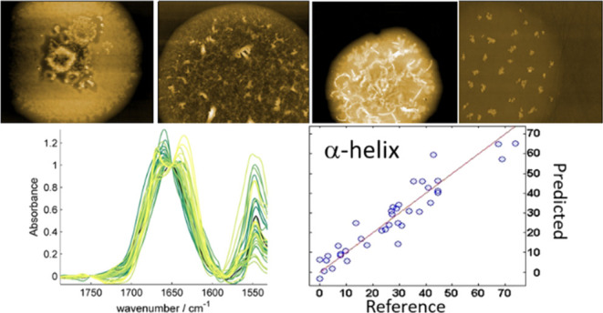
Figure 4 compares, for ASLR, the secondary structure predicted values with the “true” values obtained by analysis of the high-resolution structures obtained from PDB as described elsewhere.23 Ideally, proteins should be located on the red line (predicted values equal to the true values). For the α-helix and β-sheet structure contents, the correlation coefficients are above 0.9 for both AFMIR and μFTIR, while it is much poorer for the sum of the remaining structures, called “Others”. Prediction is better by μFTIR for the β-sheet and other structures, but for the α-helix the AFMIR and μFTIR have similar prediction errors. Importantly, for AFMIR an error of prediction of 6.39% for α-helix and 6.23% for the β-sheet structure were obtained, that is, close to many values reported in the literature for FTIR, demonstrating that AFMIR is able to predict the secondary structure of protein, though with a specific model that takes into account the specificities of the AFMIR spectra. The secondary structures of proteins can be calculated based on the AFMIR spectra and these equations
Figure 4.

Comparison of the different models obtained by FTIR and AFMIR for the different secondary structures. The first line is the results obtained by ASLR prediction for the α-helix with 7 wavenumbers (left), β-sheet with 8 wavenumbers (middle), and other structures with 8 wavenumbers (right). On the second line, the results with AFMIR data treated with SG smoothing. α-Helix is predicted with 8 wavenumbers (left), β-sheet with 8 wavenumbers (middle), and other structures with 11wavenumbers (right).
The results obtained by FTIR and AFMIR are compared in Figure S5, the predicted value from AFMIR in function of the FTIR value is plotted. All the points are observed distributed along the diagonal and no specific bias for one technique is observed.
Conclusions
The AFMIR is a recent technique with high sensibility down to single molecule and with a spatial resolution of few nanometers. Spectra obtained by AFMIR with bottom-up illumination are similar to the one obtained by FTIR. We first showed that the pure spectra of α-helix and β-sheet structure extracted by CLS are similar when obtained from AFMIR or μFTIR spectra of a 38-protein library that covers a wide range of structures. Yet, there are significant differences between the spectra obtained by these two methods, requiring the building of a specific quantitative model for predicting secondary structure from AFMIR spectra. The best model to predict the secondary structure content was found to be the ASLR model with 8 wavenumbers obtained on the data pretreated with Savitzky–Golay smoothing. The error on the prediction of the α-helix content was 6.39% (as compared to 6.52% for μFTIR) and 6.23% for β-sheet content (as compared to 5.64% for μFTIR). While slightly better models were obtained for μFTIR, the errors are of the same order of magnitude for both techniques. Quantification of protein secondary structure at the nanoscale level will open new horizons for the study of protein aggregation in cells and tissues (amyloidosis diseases). As the best prediction is based on ASLR model requiring the knowledge of the absorbance at only a few wavenumbers, it will be possible, using QCL sources, to measure rapidly AFMIR absorption maps at few specific wavenumbers that can be translated easily in secondary structure maps, saving a considerable amount of time in comparison with hyperspectral acquisition.
Acknowledgments
This work was supported by the Fonds National de la Recherche Scientifique FNRS under grant no. O001518F (EOS-Convention # 30467715). The authors thank the Walloon Region (SPW, DGO6, Belgium) for supporting the ROBOTEIN project within the frame of the EQUIP2013 Program and FNRS and Boël Sofina travel grant for the financial support.
Supporting Information Available
The Supporting Information is available free of charge at https://pubs.acs.org/doi/10.1021/acs.analchem.2c01431.
List of proteins used for the calibration and their secondary structures content, The AFMIR and μFTIR spectra of all proteins, AFM topographies of some proteins, rdCV results in PLS for LVs selections and in ASLR for wavenumbers selections, ASLR wavenumber selection for model in Figure 4 and comparison of prediction by AFMIR and FTIR (PDF)
Author Contributions
The work was designed by A.D., V.R. and E.G. J.D.M. prepared all the samples and printed the protein microarrays. J.W. recorded the AFMIR data and performed the data processing. The manuscript was written through contributions of all authors. All authors gave approval to the manuscript.
The authors declare no competing financial interest.
Supplementary Material
References
- Cerf E.; Sarroukh R.; Tamamizu-Kato S.; Breydo L.; Derclaye S.; Dufrêne Y. F.; Narayanaswami V.; Goormaghtigh E.; Ruysschaert J. M.; Raussens V. Antiparallel β-sheet: a signature structure of the oligomeric amyloid β-peptide. Biochem. J. 2009, 421, 415–423. 10.1042/bj20090379. [DOI] [PubMed] [Google Scholar]
- Celej M. S.; Sarroukh R.; Goormaghtigh E.; Fidelio G. D.; Ruysschaert J.-M.; Raussens V. Toxic prefibrillar α-synuclein amyloid oligomers adopt a distinctive antiparallel β-sheet structure. Biochem. J. 2012, 443, 719–726. 10.1042/bj20111924. [DOI] [PubMed] [Google Scholar]
- Goormaghtigh E.; Gasper R.; Bénard A.; Goldsztein A.; Raussens V. Protein secondary structure content in solution, films and tissues: redundancy and complementarity of the information content in circular dichroism, transmission and ATR FTIR spectra. Biochim. Biophys. Acta 2009, 1794, 1332–1343. 10.1016/j.bbapap.2009.06.007. [DOI] [PubMed] [Google Scholar]
- Sreerama N.; Woody R. W. Estimation of Protein Secondary Structure from Circular Dichroism Spectra: Comparison of CONTIN, SELCON, and CDSSTR Methods with an Expanded Reference Set. Anal. Biochem. 2000, 287, 252–260. 10.1006/abio.2000.4880. [DOI] [PubMed] [Google Scholar]
- Goormaghtigh E.; Raussens V.; Ruysschaert J. M. Attenuated total reflection infrared spectroscopy of proteins and lipids in biological membranes. Biochim. Biophys. Acta 1999, 1422, 105–185. 10.1016/s0304-4157(99)00004-0. [DOI] [PubMed] [Google Scholar]
- Gbaguidi B.; Hakizimana P.; Vandenbussche G.; Ruysschaert J. M. Conformational changes in a bacterial multidrug transporter are phosphatidylethanolamine-dependent. Cell. Mol. Life Sci. 2007, 64, 1571–1582. 10.1007/s00018-007-7031-0. [DOI] [PMC free article] [PubMed] [Google Scholar]
- Goormaghtigh E.; Cabiaux V.; Ruysschaert J. M. Determination of Soluble and Membrane Protein Structure by Fourier Transform Infrared Spectroscopy. Subcell. Biochem. 1994, 23, 405–450. 10.1007/978-1-4615-1863-1_10. [DOI] [PubMed] [Google Scholar]
- Baumruk V.; Pancoska P.; Keiderling T. A. Predictions of Secondary Structure using Statistical Analyses of Electronic and Vibrational Circular Dichroism and Fourier Transform Infrared Spectra of Proteins in H2O. J. Mol. Biol. 1996, 259, 774–791. 10.1006/jmbi.1996.0357. [DOI] [PubMed] [Google Scholar]
- Rahmelow K.; Hübner W. Secondary Structure Determination of Proteins in Aqueous Solution by Infrared Spectroscopy: A Comparison of Multivariate Data Analysis Methods. Anal. Biochem. 1996, 241, 5–13. 10.1006/abio.1996.0369. [DOI] [PubMed] [Google Scholar]
- Navea S.; Tauler R.; Juan A. d. Application of the local regression method interval partial least-squares to the elucidation of protein secondary structure. Anal. Biochem. 2005, 336, 231–242. 10.1016/j.ab.2004.10.016. [DOI] [PubMed] [Google Scholar]
- Goormaghtigh E.; Ruysschaert J. M.; Raussens V. Evaluation of the information content in infrared spectra for protein secondary structure determination. Biophys. J. 2006, 90, 2946–2957. 10.1529/biophysj.105.072017. [DOI] [PMC free article] [PubMed] [Google Scholar]
- Hering J. A.; Innocent P. R.; Haris P. I. An alternative method for rapid quantification of protein secondary structure from FTIR spectra using neural networks. Spectroscopy 2002, 16, 503989. 10.1155/2002/503989. [DOI] [Google Scholar]
- Dazzi A.; Prater C. B. AFM-IR: Technology and Applications in Nanoscale Infrared Spectroscopy and Chemical Imaging. Chem. Rev. 2017, 117, 5146–5173. 10.1021/acs.chemrev.6b00448. [DOI] [PubMed] [Google Scholar]
- Kurouski D.; Dazzi A.; Zenobi R.; Centrone A.. Infrared and Raman Chemical Imaging and Spectroscopy at the Nanoscale; Chemical Society Reviews, 2020. [DOI] [PMC free article] [PubMed] [Google Scholar]
- Ruggeri F. S.; Mannini B.; Schmid R.; Vendruscolo M.; Knowles T. P. J. Single molecule secondary structure determination of proteins through infrared absorption nanospectroscopy. Nat. Commun. 2020, 11, 2945. 10.1038/s41467-020-16728-1. [DOI] [PMC free article] [PubMed] [Google Scholar]
- Paluszkiewicz C.; Piergies N.; Chaniecki P.; Rękas M.; Miszczyk J.; Kwiatek W. M. Differentiation of protein secondary structure in clear and opaque human lenses: AFM - IR studies. J. Pharm. Biomed. Anal. 2017, 139, 125–132. 10.1016/j.jpba.2017.03.001. [DOI] [PubMed] [Google Scholar]
- Qin N.; Zhang S.; Jiang J.; Corder S. G.; Qian Z.; Zhou Z.; Lee W.; Liu K.; Wang X.; Li X.; Shi Z.; Mao Y.; Bechtel H. A.; Martin M. C.; Xia X.; Marelli B.; Kaplan D. L.; Omenetto F. G.; Liu M.; Tao T. H. Nanoscale probing of electron-regulated structural transitions in silk proteins by near-field IR imaging and nano-spectroscopy. Nat. Commun. 2016, 7, 13079. 10.1038/ncomms13079. [DOI] [PMC free article] [PubMed] [Google Scholar]
- Esteve E.; Luque Y.; Waeytens J.; Bazin D.; Mesnard L.; Jouanneau C.; Ronco P.; Dazzi A.; Daudon M.; Deniset-Besseau A. Nanometric chemical speciation of abnormal deposits in kidney biopsy: Infrared-nanospectroscopy reveals heterogeneities within vancomycin casts. Anal. Chem. 2020, 92, 7388–7392. 10.1021/acs.analchem.0c00290. [DOI] [PubMed] [Google Scholar]
- Ruggeri F. S.; Longo G.; Faggiano S.; Lipiec E.; Pastore A.; Dietler G. Infrared nanospectroscopy characterization of oligomeric and fibrillar aggregates during amyloid formation. Nat. Commun. 2015, 6, 7831. 10.1038/ncomms8831. [DOI] [PMC free article] [PubMed] [Google Scholar]
- Waeytens J.; Van Hemelryck V. V.; Deniset-Besseau A.; Ruysschaert J.-M.; Dazzi A.; Raussens V. Characterization by Nano-Infrared Spectroscopy of Individual Aggregated Species of Amyloid Proteins. Molecules 2020, 25, 2899. 10.3390/molecules25122899. [DOI] [PMC free article] [PubMed] [Google Scholar]
- Waeytens J.; Mathurin J.; Deniset-Besseau A.; Arluison V.; Bousset L.; Rezaei H.; Raussens V.; Dazzi A. Probing amyloid fibril secondary structures by infrared nanospectroscopy: experimental and theoretical considerations. Analyst 2020, 146, 132–145. 10.1039/D0AN01545H. [DOI] [PubMed] [Google Scholar]
- De Meutter J.; Derfoufi K.-M.; Goormaghtigh E. Analysis of protein microarrays by FTIR imaging. Biomed. Spectrosc. Imag. 2016, 5, 145–154. 10.3233/bsi-160137. [DOI] [Google Scholar]
- De Meutter J.; Goormaghtigh E. A convenient protein library for spectroscopic calibrations. Comput. Struct. Biotechnol. J. 2020, 18, 1864–1876. 10.1016/j.csbj.2020.07.001. [DOI] [PMC free article] [PubMed] [Google Scholar]
- De Meutter J.; Vandenameele J.; Matagne A.; Goormaghtigh E. Infrared imaging of high density protein arrays. Analyst 2017, 142, 1371–1380. 10.1039/c6an02048h. [DOI] [PubMed] [Google Scholar]
- De Meutter J.; Goormaghtigh E. Searching for a Better Match between Protein Secondary Structure Definitions and Protein FTIR Spectra. Anal. Chem. 2021, 93, 1561–1568. 10.1021/acs.analchem.0c03943. [DOI] [PubMed] [Google Scholar]
- De Meutter J.; Goormaghtigh E. FTIR Imaging of Protein Microarrays for High Throughput Secondary Structure Determination. Anal. Chem. 2021, 93, 3733–3741. 10.1021/acs.analchem.0c03677. [DOI] [PubMed] [Google Scholar]
- De Meutter J.; Goormaghtigh E. Evaluation of protein secondary structure from FTIR spectra improved after partial deuteration. Eur. Biophys. J. 2021, 50, 613–628. 10.1007/s00249-021-01502-y. [DOI] [PMC free article] [PubMed] [Google Scholar]
- Orengo C. A.; Michie A. D.; Jones S.; Jones D. T.; Swindells M. B.; Thornton J. M. CATH - a hierarchic classification of protein domain structures. Structure 1997, 5, 1093–1109. 10.1016/s0969-2126(97)00260-8. [DOI] [PubMed] [Google Scholar]
- Mathurin J.; Mosser G.; Dazzi A.; Deniset-Besseau A.; Schanne-Klein M.-C.; Latour G.. Correlative multiphoton microscopy and infrared nanospectroscopy of label-free collagen; Proceedings of SPIE, 2019.
- Latour G.; Robinet L.; Dazzi A.; Portier F.; Deniset-Besseau A.; Schanne-Klein M.-C. Correlative nonlinear optical microscopy and infrared nanoscopy reveals collagen degradation in altered parchments. Sci. Rep. 2016, 6, 26344. 10.1038/srep26344. [DOI] [PMC free article] [PubMed] [Google Scholar]
- Kabsch W.; Sander C. Dictionary of protein secondary structure: Pattern recognition of hydrogen-bonded and geometrical features. Biopolymers 1983, 22, 2577–2637. 10.1002/bip.360221211. [DOI] [PubMed] [Google Scholar]
- Clède S.; Lambert F.; Sandt C.; Kascakova S.; Unger M.; Harté E.; Plamont M.-A.; Saint-Fort R.; Deniset-Besseau A.; Gueroui Z.; Hirschmugl C.; Lecomte S.; Dazzi A.; Vessières A.; Policar C. Detection of an estrogen derivative in two breast cancer cell lines using a single core multimodal probe for imaging (SCoMPI) imaged by a panel of luminescent and vibrational techniques. Analyst 2013, 138, 5627–5638. 10.1039/c3an00807j. [DOI] [PubMed] [Google Scholar]
- Dazzi A.; Prater C. B.; Hu Q.; Chase D. B.; Rabolt J. F.; Marcott C. AFM-IR: Combining Atomic Force Microscopy and Infrared Spectroscopy for Nanoscale Chemical Characterization. Appl. Spectrosc. 2012, 66, 1365–1384. 10.1366/12-06804. [DOI] [PubMed] [Google Scholar]
- Savitzky A.; Golay M. J. E. Smoothing and Differentiation of Data by Simplified Least Squares Procedures. Anal. Chem. 1964, 36, 1627–1639. 10.1021/ac60214a047. [DOI] [Google Scholar]
- Dousseau F.; Pezolet M. Determination of the secondary structure content of proteins in aqueous solutions from their amide I and amide II infrared bands. Comparison between classical and partial least-squares methods. Biochemistry 1990, 29, 8771–8779. 10.1021/bi00489a038. [DOI] [PubMed] [Google Scholar]
- Filzmoser P.; Liebmann B.; Varmuza K. Repeated double cross validation. J. Chemom. 2009, 23, 160–171. 10.1002/cem.1225. [DOI] [Google Scholar]
- Barth A.; Haris P. I.; Goormaghtigh E. FTIR Data Processung and Analysis Tools. Adv. Biomed. Spectrosc. 2009, 2, 104–128. 10.3233/978-1-60750-045-2-104. [DOI] [Google Scholar]
- Goormaghtigh E.Infrared Spectroscopy: Data Analysis. In Encyclopedia of Biophysics; Roberts G. C. K., Ed.; Springer Berlin Heidelberg: Berlin, Heidelberg, 2013; pp 1049–1057. [Google Scholar]
- Lasch P. Spectral pre-processing for biomedical vibrational spectroscopy and microspectroscopic imaging. Chemom. Intell. Lab. Syst. 2012, 117, 100–114. 10.1016/j.chemolab.2012.03.011. [DOI] [Google Scholar]
- Barth A. Infrared spectroscopy of proteins. Biochim. Biophys. Acta 2007, 1767, 1073–1101. 10.1016/j.bbabio.2007.06.004. [DOI] [PubMed] [Google Scholar]
Associated Data
This section collects any data citations, data availability statements, or supplementary materials included in this article.