Oxyhemoglobin and cerebral blood flow transients detect infarction in rat focal brain ischemia

Abstract

Spreading depolarizations (SD) refer to the near-complete depolarization of neurons that is associated with brain injuries such as ischemic stroke. The present gold standard for SD monitoring in humans is invasive electrocorticography (ECoG). A promising non-invasive alternative to ECoG is diffuse optical monitoring of SD-related flow and hemoglobin transients. To investigate the clinical utility of flow and hemoglobin transients, we analyzed their association with infarction in rat focal brain ischemia. Optical images of flow, oxy-hemoglobin, and deoxy-hemoglobin were continuously acquired with Laser Speckle and Optical Intrinsic Signal imaging for 2 hours after photochemically induced distal middle cerebral artery occlusion in Sprague-Dawley rats (n=10). Imaging was performed through a 6×6 mm window centered 3 mm posterior and 4 mm lateral to Bregma. Rats were sacrificed after 24 hours, and the brain slices were stained for assessment of infarction. We mapped the infarcted area onto the imaging data and used nine circular regions of interest (ROI) to distinguish infarcted from non-infarcted tissue. Transients propagating through each ROI were characterized with six parameters (negative, positive, and total amplitude; negative and positive slope; duration). Transients were also classified into three morphology types (positive monophasic, biphasic, negative monophasic). Flow transient morphology, positive amplitude, positive slope, and total amplitude were all strongly associated with infarction (p<0.001). Associations with infarction were also observed for oxy-hemoglobin morphology, oxy-hemoglobin positive amplitude and slope, and deoxy-hemoglobin positive slope and duration (all p<0.01). These results suggest that flow and hemoglobin transients accompanying SD have value for detecting infarction.

INTRODUCTION

Spreading depolarizations (SD) is the term for the near-complete depolarization of neurons (Somjen 2001; Dreier 2011) accompanied by the decrease of membrane resistance (Czeh, Aitken, and Somjen 1993), the loss of electrical activity (Leao 1944), neuronal swelling and distortion of dendritic spines, (Takano et al. 2007) (Risher, Andrew, and Kirov 2009) and cytotoxic edema (Nicholson et al. 1978; Takano et al. 2007). Furthermore, SD involves astrocytes (Peters et al. 2003; Chuquet, Hollender, and Nimchinsky 2007; Urbach, Brueckner, and Witte 2015; Largo et al. 1996), stimulates microglial cells and inflammasome formation, and activates cytokine gene expression (Jander et al. 2001; Walsh, Muruve, and Power 2014). SD is responsible for necrotic and selective neuronal lesion evolution in gray matter as reported in diverse disease models and species (Hartings et al. 2017; Lauritzen et al. 2011). There is a strong clinical experience that SD is associated with brain injuries such as ischemic stroke, subarachnoid hemorrhage, and traumatic brain injury (Hartings et al. 2011; Lückl et al. 2018; Dohmen et al. 2008; Dreier et al. 2022). Accordingly, the Co-Operative Studies on Brain Injury Depolarizations (COSBID) Group recommends routine monitoring of SD for brain-injured patients (Dreier et al. 2017).

The present gold standard for detection of SD in human is electrocorticography (ECoG) with a linear subdural platinum electrode strip. ECoG, however, has the disadvantage of allowing only invasive measurement of SDs in patients, and it does not provide information on hemodynamic changes. To overcome these challenges, the consensus article of COSBID concludes that the use of non-invasive technologies such as continuous scalp electroencephalography (EEG) and optical hemodynamic imaging (e.g., near-infrared spectroscopy or diffuse correlation spectroscopy) hold promise (Dreier et al. 2017).

In animal models of stroke, the optical techniques of laser Doppler (LD) and laser speckle imaging (LSI) have been used to measure regional cerebral blood flow (CBF) related to SDs (Hossmann 1996) (Dunn et al. 2001). Additionally, optical intrinsic signal (OIS) imaging enables the measurement of regional oxy-hemoglobin and deoxy-hemoglobin concentrations (Jones et al. 2001), and strong correlations between ECoG changes and LSI/LD/OIS metrics have been demonstrated (Peixoto, Fernandes de Lima, and Hanke 2001; Dahlem and Müller 1997; Obrenovitch, Chen, and Farkas 2009; Lückl et al. 2012).

In our work, we sought to investigate whether these cortical hemoglobin and flow transients that accompany SD have value for detecting infarction in a rat focal brain ischemia model. Continuous 2D topographic maps of cortical oxy- and deoxy-hemoglobin were measured with OIS (Dunn et al. 2003; Grinvald, Lieke, et al. 1986). Corresponding topographic maps of cortical blood flow were measured in parallel with LSI (Dunn et al. 2001). We hypothesized that different parameters (amplitude, durations, slopes and shapes) of the hemoglobin and flow transients captured from these images are associated with infarction. To answer the hypothesis, we analyzed the animals of a prospective study (n=10) with dichotomized histological outcomes. A positive result preclinically motivates future translational research on the development of near-infrared spectroscopy and diffuse correlation spectroscopy biomarkers of injury in humans with ischemic stroke.

EXPERIMENTAL PROCEDURES

Photochemically induced distal middle cerebral artery occlusion.

All procedures performed were approved by the Institutional Animal Care and Use Committee of the University of Pennsylvania. Mature, adult male Sprague–Dawley rats (n=10, 290–320 g, ~12-13 weeks of age) were anesthetized with 4% isoflurane for induction in a mixture of 50% nitrous oxide and 50% oxygen and maintained on 1.2–1.3% isoflurane (1.0–1.25 MAC) in 70% nitrous oxide and 30% oxygen during surgery and throughout the study. Body temperature was monitored by a rectal probe and maintained at 37.5 ± 0.2°C with a heating blanket regulated by a homeothermic blanket control unit (Harvard Apparatus Limited Holliston, MA, USA). A polyethylene catheter (PE-50) was placed into the tail artery for the measurement of arterial blood pressure and for blood gas sampling. Blood pressure was continuously monitored using a pressure transducer and recorded on a computer-based recording system (PowerLab, ADInstruments, Colorado Springs, CO, USA). The right common carotid artery was exposed by a ventral midline incision in the neck and the retraction of the sternocleidomastoid muscle. The exposed artery was surrounded by a snare. Of note, care was taken to avoid trauma to the vagal nerve while dissecting the carotid sheath (this was facilitated by our use of the photochemically induced ischemia model, which only requires the exposure of a short section of the common carotid artery).

The rats were placed into a stereotaxic head holder, and a 6 × 6 mm area centered 3 mm posterior and 4 mm lateral to Bregma was uniformly thinned to translucency for optical imaging (Figure 1). To reduce specular reflections, ultrasound gel was applied to the thinned skull and a glass coverslip placed on top. Special attention was paid during surgical preparation to make the skull thickness uniform (Parthasarathy et al. 2008). To induce middle cerebral artery (MCA) occlusion, a 2-cm vertical incision was made midway between the right eye and the right ear. The temporalis muscle was separated and retracted to expose the zygomatic and squamosal bones. Under an operating microscope (Carl Zeiss, Inc.), a burr hole of 4 mm in diameter was made with a high-speed drill 1 mm rostral to the anterior junction of the zygomatic and squamosal bones, revealing the distal segment of the MCA. The epidural temperature was monitored by probe and maintained at 37.5 ± 0.3°C with a custom-made air delivery blowing warm air on the dura.

Figure 1.

Experimental setup. A. Laser Speckle Imaging (LSI) and multispectral Optical Intrinsic Signal (OIS) imaging were used to acquire topographic images (with a CCD camera) of cortical cerebral blood flow (CBF), oxy-hemoglobin (Oxy-Hb), and deoxy-hemoglobin (Deoxy-Hb) once every two seconds. B. Diagram of the rat brain showing the 6 × 6 mm thinned part of the skull for hemodynamic imaging (blue square). Illumination from a laser (532 nm wavelength) produced a thrombus proximally to the Y-shaped juncture of the frontal and parietal branches of the middle cerebral artery.

The right side of the stereotaxic frame was tilted upward to facilitate the focusing of the beam from a 4 mW diode laser (532 nm wavelength, LaserGlow Technologies, model LRS-0532-KFM-00030-03) on the exposed MCA (a spherical lens of 25 cm focal length was used for focusing). A stock solution of Erythosin B dye (MP Biomedicals, Solon, OH, USA), 17 mg/mL in 0.9% saline, was then injected intravenously (via the tail vein) at a dose of 40 mg/kg.

Immediately after injection of the dye, the MCA was irradiated with the diode laser. The irradiation produced a thrombus proximally to the Y-shaped juncture of the frontal and parietal branches of the MCA. An orange fluorescence was immediately observed in the irradiated distal MCA segment under the operating microscope. A white thrombus began to form approximately 4–5 min later within the fluorescent segment and gradually elongated distally. Following the irradiation, the right CCA was also occluded by tightening the snare.

Changes in oxygenation and blood flow were monitored through the thinned skull preparation with optical intrinsic signal imaging (OIS) (Grinvald, Segal, et al. 1986) (Kohl et al. 2000) and laser speckle imaging (LSI) (Briers 2001; Dunn et al. 2001; Durduran et al. 2004).

Cerebral Hemodynamic Imaging

The techniques of LSI and OIS were combined to longitudinally acquire 2D images of cortical blood flow (CBF), oxy-hemoglobin (Oxy-Hb), and deoxy-hemoglobin (Deoxy-Hb). A schematic of the instruments used to acquire the data is shown in Figure 1, and technical details of the instrument are described elsewhere(Baker et al. 2013). Note that two sets of illumination sources were used for OIS. For the first 5 animals imaged, a xenon arc lamp was directed through a filter wheel (Luckl et al. 2010). For the last 5 animals imaged, OIS illumination was performed with three collimated light emitting diodes (LEDs)(Baker et al. 2013). With this instrument, we sequentially acquired one three-wavelength set of OIS images and 15 LSI images every 2 s.

OIS and LSI imaging was performed from 5-minutes prior to 2-hours after the initiation of MCA occlusion in 15-minute-long sequences (there was approximately 10-20 seconds between the 15-minute-long sequences). For LSI analysis, a 7×7 pixel sliding window was employed to calculate speckle contrast images, which were then converted to speckle CBF images based on an assumed Lorentzian velocity distribution of the moving red blood cells (Zhou et al. 2008). To improve SNR, 15 speckle CBF images were averaged to obtain one CBF image every 2 s. Relative CBF was obtained by normalizing the CBF index images by the mean CBF index image during the 5-minute pre-occlusion baseline with a correction for biological zero (Zhou et al. 2008).

For OIS, differential changes in Oxy-Hb and Deoxy-Hb relative to their average levels during the first minute after MCA occlusion were computed via the modified Beer-Lambert law (Baker et al. 2013; Kohl et al. 2000; Dunn et al. 2003). (Note, with the modified Beer-Lambert law, computing changes relative to a pre-occlusion baseline is not feasible because the method breaks down for the large hemoglobin decreases that accompany occlusion (Jones et al. 2008)) Finally, a 5-by-5 pixel sliding spatial Gaussian filter was applied to the relative CBF, Oxy-Hb, and Deoxy-Hb images to improve SNR.

Mapping of Infarcted Tissue to the LSI and OIS Images

Tissue staining with 2% diphenyltetrazolium chloride (TTC) at 24 h after MCA occlusion has been established as an excellent marker of the extent of brain tissue damage (Bederson et al. 1986; Bardutzky et al. 2005). Accordingly, at 24 h after MCA occlusion, the animals were sacrificed. The brain was removed from the skull and was sectioned in the coronal plane at 1.5-mm intervals using a rodent brain matrix. The brain slices were stained with TTC and photographed, and the cortical infarct volume was determined as described previously (Luckl, Keating, and Greenberg 2008). The distance between the midline and the border of the infarct zone on the TTC slices was measured and mapped onto the LSI and OIS images individually in each animal (see Figure 2). Specifically, a high-resolution laser Speckle contrast image (obtained prior to MCA occlusion) was used for the mapping, which clearly showed the blood vessels (Dunn et al. 2001). For the comparison of transients propagating in infarcted versus non-infarcted tissue, nine circular regions of interest (ROI, 0.3 mm in diameter) were used. The Speckle contrast image was divided into nine equal sectors, and one ROI was placed in each sector (see Figure 2). Six ROIs (i.e., #1-6) were placed in the infarct zone, while the remaining three ROIs (i.e., #7-9) were placed in non-infarcted tissue. Care was taken to ensure the ROIs were not over any large blood vessels.

Figure 2.

Mapping the layout of ROIs with the border of the infarcted tissue in a representative animal. Slices of TTC staining can be seen in the left panel. Four slices (4x1.5 mm) marked with the letter “W” are under the 6 × 6 mm optical imaging window. The black circles depict the positions of each ROI (1-9) on a laser Speckle contrast image (6x6 mm) in the right panel. The black triangles represent the border between the infarcted (ROI 1-6) and non-infarcted territory (ROI 7-9) both on the TTC slices and laser Speckle contrast image. The relative, spatial position of the “optical window” to Bregma and from midline (1 mm) is illustrated below the panel on the right.

Analysis of Transients

As described in the previous section, transients were identified and characterized from the image data via analysis of nine spatial ROIs (see Figure 2). Relative CBF, Oxy-Hb, and Deoxy-Hb at each ROI were plotted vs. time. The temporal plots were manually reviewed to identify hemodynamic transients.

Transients were identified by their propagating feature (e.g., an increased relative CBF wave seen in at least two ROIs with appropriate time delay). Once identified, transients were categorized as Type I, Type II, or Type III. Type I transients are positive monophasic (have a positive amplitude only), Type II transients are biphasic (have a negative and positive amplitude), and Type III transients are negative monophasic (have a negative amplitude only) (see Figure 3). Then, for a given ROI, baseline relative CBF, ΔOxy-Hb, and ΔDeoxy-Hb levels for each transient were determined by taking their mean values across the 5-s window prior to the transient’s start. Recall, as described in the Cerebral Hemodynamic Imaging section, relative CBF is the speckle CBF index normalized by its pre-occlusion level; ΔOxy-Hb and ΔDeoxy-Hb are differential concentration changes relative to the first minute after MCA occlusion in μM.

Figure 3.

Representative traces of different types (I, II, III) of transients. The duration (grey line) of the transients were determined as the time at which the average signal intercrossed with the ascending or the descending leg of the transients. The amplitude denotes the peak magnitude change in relative cerebral blood flow (%), oxy-hemoglobin concentration (μM), or deoxy-hemoglobin concentration (μM). The negative amplitude (NAmp, blue vertical line) and positive amplitude (PAmp, red vertical line) were measured separately. We also calculated the slope of the positive and negative amplitudes. The positive and negative slopes (Pslope and Nslope) are the amplitudes divided by the preceding temporal durations indicated by the green horizontal lines. Finally, the total amplitude (TAmp) is defined as PAmp, PAmp+NAmp, and NAmp for the type I, II, and III transients, respectively.

For CBF transients of Type I and Type II, the maximum relative CBF levels during the transients were identified. The positive relative CBF amplitude (CBF PAmp) is the difference between the transient’s maximum level and its baseline level. The positive CBF slope (CBF Pslope) is defined as the CBF PAmp divided by the time it takes CBF to reach the CBF PAmp level from its baseline level (see Figure 3). For CBF transients of Type II and Type III, the minimum relative CBF levels during the transients were identified. The negative CBF amplitude (CBF NAmp) is the difference between the transient’s baseline level and its minimum level. The negative CBF slope (CBF Nslope) is defined as the CBF NAmp divided by the time it takes CBF to reach the CBF NAmp level from its baseline level (see Figure 3). The PAmp, Pslope, NAmp, and Nslope parameters are defined the same way for Oxy-Hb and Deoxy-Hb transients (e.g., Oxy-Hb PAmp is the difference between the transient’s maximum ΔOxy-Hb level and its baseline level).

Finally, a TAmp parameter was determined for each transient: for transients of Type I, TAmp = PAmp; for transients of Type II, TAmp = PAmp + NAmp (i.e., the peak-to-peak height); and for transients of Type III, TAmp = NAmp. In addition, the duration of each transient was determined, which was the difference between the start time and end time of the transient (start and end times were determined by the times at which the signal intercrossed with the ascending and the descending leg of the transient, see Figure 3). Of note, some transients did not return to their baseline levels at all, while others did not return to their baseline levels by the end the 15-minute-long sequence of LSI/OIS acquisition (recall, LSI/OIS imaging was performed in sequential 15-minute-long sequences with ~10-20 seconds between sequences). For these transients, duration could not be measured.

Statistical analysis

Statistical calculations were performed with SPSS version 26 (IBM Corporation). All statistical tests were 2-sided, and p < 0.05 was considered to indicate significance. We assessed whether the CBF transient characterization parameters (i.e., NAmp, PAmp, TAmp, duration, Nslope, Pslope) differed between the infarcted and non-infarcted tissue regions. Specifically, we used a mixed-model ANOVA (Brown H 1999) to compare the means of these characterization parameters between ROIs in the infarcted tissue (i.e., ROIs #1-6) and ROIs in the non-infarcted tissue (i.e., ROIs #7-9). For each animal, the characterization parameters in each infarcted ROI (i.e., ROIs #1-6) were used as a separate datapoint for infarcted tissue in the comparison. Likewise, the characterization parameters in each non-infarcted ROI (i.e., #7-9) were used as a separate datapoint for non-infarcted tissue. The mixed-model ANOVA accounts for the lack of independence across the multiple infarcted and non-infarcted ROIs from each animal. The model further accounts for the lack of independence across multiple transients occurring in the same animal. Mixed-model ANOVA was also used to compare the means of the analogous Oxy-Hb and Deoxy-Hb transient characterization parameters between the infarcted and non-infarcted tissue regions. Finally, the estimated mean and the standard error of the estimated mean obtained from the mixed-model ANOVA is reported for each characterization parameter.

We were also interested in differences between the occurrence frequency of transient types that propagated across infarcted versus non-infarcted tissue. First, we computed the number of each CBF transient type propagating across infarcted tissue as a percentage of the total number of CBF transients (of all types) detected. The analogous percentages for non-infarcted tissue, and for the Oxy-Hb and Deoxy-Hb transients, were also computed. Next, we computed the odds ratios (OR) for infarction of each CBF, Oxy-Hb, and Deoxy-Hb transient type. To assess whether the odds across transient types were significantly different from each other, a generalized mixed logistic regression model with binary matched pairs was used (Brown H 1999). The following estimated ratios (with 95% confidence intervals) were obtained from the model: OR (Type III vs. Type I) and OR(Type II vs. Type I). The mixed logistic regression model accounts for the lack of independence between transients from the same animal.

Summary statistics are presented using means and standard deviations for: 1) the cortical infarct volume; 2) the spatially averaged relative CBF across the infarcted ROIs (#1-6) immediately after MCA occlusion; 3) the spatially averaged relative CBF across the non-infarcted ROIs (#7-9) immediately after MCA occlusion; 4) the number of CBF transients per animal; and 5) the CBF, Oxy-Hb, and Deoxy-Hb transient characterization parameters (i.e., NAmp, PAmp, TAmp, duration, Nslope, Pslope) across the non-infarcted and across the infarcted tissue regions.

RESULTS

For all animals (n = 10), the physiological variables (blood pressure, blood gas, core and epidural temperature) measured remained within normal ranges for the 2 hours of monitoring after MCA occlusion. The average cortical infarct volume across animals was 109 ± 39 mm³. CBF, Oxy-Hb, and Deoxy-Hb transients in an exemplar animal are shown in Figure 4. In total, across all animals and all 9 ROIs, 285 CBF transients, 234 Oxy-Hb transients, and 196 Deoxy-Hb transients were analyzed. Of these totals, the percentages of each transient type in infarcted and non-infarcted tissue regions are reported in Table 1.

Figure 4.

Example temporal traces of relative cerebral blood flow (rCBF; top row), change in oxy-hemoglobin concentration (red curve; bottom row), and change in deoxy-hemoglobin concentration (blue curve; bottom row) at 3 regions of interest (ROI; as illustrated in Figure 5, #2 and #5 are in the infarct region, #8 is in the non-infarct region) in the same animal. Time-zero is immediately after middle cerebral artery occlusion. rCBF is the percentage of the pre-occlusion CBF level, and the differential hemoglobin concentration changes (Δ) are relative to the average levels during the first minute after occlusion. Note, the vertical axis scale for ROI 8 is different from that for ROIs 2 and 5.

Table 1.

Summary of the spatial distributions (% of total) for the different types of cerebral blood flow (CBF), oxyhemoglobin (Oxy-Hb), and deoxy-hemoglobin (Deoxy-Hb) transients. The total number of CBF, Oxy-Hb, and Deoxy-Hb transients were 285, 234, and 196, respectively.

TYPES	CBF	Oxy-Hb	Deoxy-Hb
	INFARCTED
I	15 %	3.8 %	24 %
II	13 %	10 %	14 %
III	21 %	31 %	7.3 %
	NON-INFARCTED
I	35 %	22 %	29 %
II	16 %	29 %	9.9 %
III	0.7 %	3.8 %	17 %

Of note, unanticipated transient malfunctions in the OIS instrumentation occurred in two animals, which resulted in the loss of 15 minutes of OIS data post-occlusion for each animal. During these two intervals of OIS data loss, 16 CBF transients were detected. There were an additional 35 CBF transients for which accompanying Oxy-Hb and Deoxy-Hb transients were not detected. The mismatch rate between the CBF and Oxy-Hb transients was 62% (22/35) over the infarcted area. Finally, for 38 of the detected Oxy-Hb transients, accompanying Deoxy-Hb transients were not detected. The magnitude of the mismatch between the Oxy-Hb and Deoxy Hb transients proved to be 44% (17/38) over the infarcted area.

Cerebral blood flow and flow transients

Immediately after MCA occlusion, the average relative CBF (fraction of pre-occlusion CBF) in the infarcted and non-infarcted regions were 34±13% and 51±11%, respectively. As expected, the post-occlusion CBF in the infarcted region was lower (p<0.001). We detected 5.2±2.2 propagating CBF transients per animal. Of the total number of transients analyzed, 48% were in the infarcted tissue, and 52% were in the non-infarcted tissue. The flow transients propagated across tissue in multiple directions. Most transients (71%) propagated from frontal to caudal (either lateral-medial or medial-lateral). The remainder of transients propagated in the reverse direction, i.e., from caudal to frontal.

The PAmp, TAmp and Pslope CBF transient characterization parameters were higher in the non-infarcted tissue than the infarcted tissue (p<0.001 for all 3 parameters) (Table 2, Figure 5). There was no difference in the other three characterization parameters between non-infarcted and infarcted tissue.

Table 2.

Summary of the descriptive statistics of the cerebral blood flow (CBF) transient characterization parameters (negative amplitude (NAmp, %), positive amplitude (PAmp, %), total amplitude (Tamp, %), duration (second), negative slope (Nslope, NAmp/second), and positive slope (Pslope, PAmp/second) are defined in Figure 3 and in the Analysis of Transients subsection). Both the experimental mean and standard deviation, as well as the estimated mean and standard error of the estimated mean from the mixed ANOVA model, are reported. The p values are from the mixed ANOVA model comparison of infarcted to non-infarcted tissue. PAmp, TAmp and Pslope were associated with infarction.

CBF		NAmp	PAmp	TAmp	Duration	NSlope	PSlope
INFARCTED	Mean	13.74	10.13	15.54	149.83	0.48	0.16
	Std. Deviation	7.32	8.56	10.86	71.85	0.33	0.15
	Estimated Mean	13.93	9.87	15.15	151.04	0.46	0.16
	Std. Error of Estimated Mean	0.98	2.11	1.78	9.89	0.04	0.04
NON-INFARCTED	Mean	11.49	31.64	34.60	183.58	0.57	0.60
	Std. Deviation	7.08	18.69	19.45	70.07	0.38	0.37
	Estimated Mean	11.41	30.10	32.85	182.73	0.54	0.58
	Std. Error of Estimated Mean	1.34	1.83	1.98	11.13	0.06	0.04
STATISTICS	p-values	0.14	<0.001	<0.001	0.07	0.32	<0.001

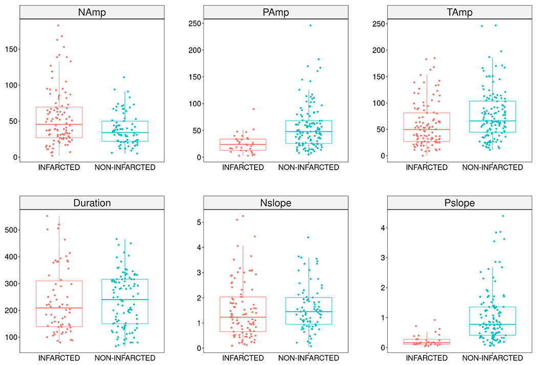
Figure 5.

Spatial distributions (INFARCTED vs NON-INFARCTED) of the different characterization parameters of the cerebral blood flow transients. Boxplots show the median and interquartile range of the characterization parameter on the vertical axis. The negative amplitude (n=141) (NAmp, %), positive amplitude (n=226) (PAmp, %), total amplitude (n=285) (Tamp, %), duration (n=255) (second), negative slope (n=136) (Nslope, NAmp/second), and positive slope (n=220) (Pslope, PAmp/second) are defined in Figure 3 and in the Analysis of Transients subsection. PAmp, Tamp, and Pslope were higher in the non-infarcted tissue than the infarcted tissue (p < 0.001 for all three comparisons). There was no difference between non-infarcted and infarcted tissue in the other parameters.

CBF transient type was also associated with infarction (p < 0.001). Further, the generalized mixed logistic regression model estimated that the odds of infarction for Type III are 40.6 and 25.0 times higher than the corresponding odds for Type I and Type II, respectively (i.e., OR (Type III vs. Type I) = 40.6, OR (Type III vs. Type I) = 25.0). Accordingly, Type III transients were much more common in infarcted tissue than the other transient types.

Oxyhemoglobin transients

The oxy-hemoglobin transients shared several similarities with the CBF transients. Of the total number of transients analyzed, 45% were in the infarcted tissue and 55% were in the non-infarcted tissue. The PAmp (p = 0.007) and Pslope (p = 0.001) parameters were higher in the non-infarcted tissue than the infarcted tissue (Table 3, Figure 6). Note, however, that in contrast to CBF transients, the Oxy-Hb TAmp parameter was not associated with infarction. The other transient characterization parameters were also not associated with infarction.

Table 3.

Summary of the descriptive statistics of the oxy-hemoglobin (Oxy-Hb) transient characterization parameters (negative amplitude (NAmp, μM), positive amplitude (PAmp, μM), total amplitude (Tamp, μM), duration (second), negative slope (Nslope, NAmp/second), and positive slope (Pslope, PAmp/second) are defined in Figure 3 and in the Analysis of Transients subsection). Both the experimental mean and standard deviation, as well as the estimated mean and standard error of the estimated mean from the mixed ANOVA model, are reported. The p values are from the mixed ANOVA model comparison of infarcted to non-infarcted tissue. PAmp and PSlope were associated with infarction.

Oxy-Hb		NAmp	PAmp	TAmp	Duration	NSlope	PSlope
INFARCTED	Mean	55.46	25.58	60.29	236.64	1.51	0.24
	Std. Deviation	38.94	17.70	42.23	122.94	1.12	0.21
	Estimated Mean	54.33	27.70	57.84	239.61	1.44	0.25
	Std. Error of Estimated Mean	5.19	7.99	6.35	14.66	0.15	0.17
NON-INFARCTED	Mean	38.70	57.12	77.10	237.77	1.78	1.04
	Std. Deviation	22.27	40.97	46.84	99.53	1.74	0.89
	Estimated Mean	39.21	55.57	75.10	235.82	1.58	0.99
	Std. Error of Estimated Mean	6.49	5.88	6.93	12.61	0.17	0.12
STATISTICS	p- values	0.14	<0.001	0.07	0.85	0.52	<0.001

Figure 6.

Spatial distributions (INFARCTED vs NON-INFARCTED) of the different characterization parameters of the oxy-hemoglobin transients. Boxplots show the median and interquartile range of the characterization parameter on the vertical axis. The negative amplitude (n=185) (NAmp, μM), positive amplitude (n=153) (PAmp, μM), total amplitude (n=234) (Tamp, μM), duration (n=169) (second), negative slope (n=174) (Nslope, NAmp/second), and positive slope (n=146) (Pslope, PAmp/second) are defined in Figure 3 and in the Analysis of Transients subsection. PAmp (p = 0.007) and Pslope (p = 0.001) were higher in the non-infarcted tissue than the infarcted tissue. There was no difference between non-infarcted and infarcted tissue in the other parameters.

Oxy-Hb transient type was associated with infarction (p < 0.001). The generalized mixed logistic regression model estimated that the odds of infarction for Type III are 29.8 and 20.7 times higher than the corresponding odds for Type I and Type II, respectively (i.e., OR (Type III vs. Type I) = 29.8, OR (Type III vs. Type I) = 20.7). Thus, as with the CBF transient type, Type III transients were more common in infarcted tissue than the other transient types.

Deoxyhemoglobin transients

Of the total number of Deoxy-Hb transients analyzed, 45% were in the infarcted tissue and 55% were in the non-infarcted tissue. Compared to the infarcted tissue, the Pslope parameter was higher (p = 0.007) and the duration parameter was lower (p<0.001) in the non-infarcted tissue (Table 4, Figure 7). None of the other characterization parameters analyzed were associated with infarction. In addition, Deoxy-Hb transient type was not associated with infarction (p = 0.5).

Table 4.

Summary of the descriptive statistics of the deoxy-hemoglobin (Deoxy-Hb) transient characterization parameters (negative amplitude (NAmp, μM), positive amplitude (PAmp, μM), total amplitude (Tamp, μM), duration (second), negative slope (Nslope, NAmp/second), and positive slope (Pslope, PAmp/second) are defined in Figure 3 and in the Analysis of Transients subsection). Both the experimental mean and standard deviation, as well as the estimated mean and standard error of the estimated mean from the mixed ANOVA model, are reported. The p values are from the mixed ANOVA model comparison of infarcted to non-infarcted tissue. Duration and Pslope were associated with infarction.

Deoxy-Hb		NAmp	PAmp	TAmp	Duration	NSlope	PSlope
INFARCTED	Mean	16.41	20.76	24.43	211.74	0.59	0.29
	Std. Deviation	17.62	12.08	17.84	75.78	0.55	0.21
	Estimated Mean	16.31	20.84	24.23	211.68	0.57	0.29
	Std. Error of Estimated Mean	2.34	1.55	1.86	8.86	0.08	0.05
NON-INFARCTED	Mean	19.88	22.51	24.96	153.60	0.59	0.55
	Std. Deviation	8.99	13.22	14.96	63.58	0.32	0.48
	Estimated Mean	19.68	22.14	24.73	153.58	0.58	0.55
	Std. Error of Estimated Mean	2.25	1.62	1.77	8.44	0.08	0.05
STATISTICS	p- values	0.31	0.57	0.85	<0.001	0.92	<0.001

Figure 7.

Spatial distributions (INFARCTED vs NON-INFARCTED) of the different characterization parameters of the deoxy-hemoglobin transients. Boxplots show the median and interquartile range of the characterization parameter on the vertical axis. The negative amplitude (n=93) (NAmp, μM), positive amplitude (n=150) (PAmp, μM), total amplitude (n=196) (Tamp, μM), duration (n=154) (second), negative slope (n=89) (Nslope, NAmp/second), and positive slope (n=141) (Pslope, PAmp/second) are defined in Figure 3 and in the Analysis of Transients subsection. Compared to the infarcted tissue, duration (p < 0.001) was lower and Pslope (p = 0.007) was higher in the non-infarcted tissue. There was no difference between non-infarcted and infarcted tissue in the other parameters.

DISCUSSION

Our study provides multispectral and multimodal (LSI+OIS) imaging data about the spatial distribution of both flow-and hemoglobin transients in a focal brain ischemia model of the rat. Notably, we identified several variables of these transients which distinguished injured versus non-injured territories in ischemic stroke. The transient type (I-III), and the positive slope of the transients, appear to hold particular promise for translational research of acute brain injuries. Thus, regional heterogeneity of the transients detected by optical imaging might serve as a noninvasive hemodynamic and functional biomarker of the underlying cortex.

Flow transients

We observed in 2009 that the shape of flow transients is highly diverse in rat focal cerebral ischemia (Luckl et al. 2009). Spatial trends in spreading depression related flow transients have also been observed during focal ischemia in cats (Strong et al. 2007), swine (Schöll et al. 2017), and mice (Shin et al. 2006). Although to our knowledge, such spatial trends have not yet been directly observed in humans, case examples of heterogeneous CBF responses to SDs have been detected with invasive ECoG and CBF monitoring in subarachnoid hemorrhage patients (Dreier et al. 2009). These studies motivated us to rigorously compare spatial differences in flow transients propagating in tissue dichotomized by histological outcome. We found that hypoperfusive transients (type III) are associated mostly with the infarcted region while the hyperemic transients (type I) are characteristic for non-infarcted regions.

The continuum of hemodynamic responses to SDs encompasses transient events from hyperemia to hypoperfusion. It is known that peak hyperemia is characteristic for a healthy tissue in most species(Ayata and Lauritzen 2015). Accordingly, we primarily observed hyperemic transients in rats over the non-injured territory with relatively higher post-occlusive CBF values. However, a hypoperfusive response - a spreading ischemia – dominates the injured territories with lower post-occlusive CBF values. This inverse, hemodynamic response has been observed in a model mimicking the situation after aneurysmal subarachnoid bleeding(Dreier et al. 1998), in which artificial cerebrospinal fluid with an elevated K+ concentration together with NO scavenger hemoglobin were topically applied to the cerebral cortex. Similar conditions due to elevated extracellular potassium concentration and reduced NO synthesis are likely present after arterial occlusion(Lemale et al. 2022). In a vicious circle, spreading ischemia further deteriorates perfusion in the underlying brain tissue.

Three out of six characterization variables of the flow transients exhibited significant spatial heterogeneity in our study. To our surprise, Pslope, proved to be an excellent indicator for viable tissue. Similarly, a positive correlation between the resting state rCBF and PSlope was observed in another rat ischemia study(Feuerstein et al. 2014). The authors considered Pslope as the functional marker of the capacity to raise CBF. The strong associations of the other two variables (PAmp, TAmp) with infarction observed herein are consistent with the findings of our prior studies that used residual blood flow after MCA occlusion as a proxy of infarction. Specifically, in rat focal brain ischemia, we identified positive correlations between the residual blood flow and the average amplitude of the positive and negative peaks of the transients (Luckl et al. 2009) (Lückl et al. 2012).

Summarizing our results in context with the abundant literature of this field, we conclude that the flow transient is a good candidate for noninvasive monitoring of SDs in translational research.

Oxy-and deoxyhemoglobin transients

Analogously to the flow transients, the oxy-hemoglobin transients manifested typically as a monophasic decrease in the oxy-hemoglobin concentration (type III) over the infarcted region, while biphasic changes (type II) or monophasic increase (type I) were characteristic over the non-infarcted region. An opposite but not significant trend was observed with the deoxy-hemoglobin transients. These morphology findings are supported by a previous OIS/LSI imaging study of six mice after distal MCA occlusion (Jones et al. 2008). In this study, three regions (core, penumbra, non-ischemic) were identified based on residual CBF measurements, and oxy- and deoxy-hemoglobin transients were observed. Although histological outcome was not determined in this study, and a statistical comparison of transient morphology across regions was not done, the authors showed case examples of hemoglobin trends with similar spatial trends to those reported herein. Case examples of similar spatial patterns in total hemoglobin transients (estimated from OIS intensity images at a single wavelength) were also observed in swine and rat focal ischemia models (Bere et al. 2014; Schöll et al. 2017). Finally, evidence of heterogeneous oxygenation responses to SDs were observed with invasive ECoG and local brain tissue oxygen tension monitoring in humans with subarachnoid hemorrhage (Winkler et al. 2017).

SD increases metabolism and oxygen demand in brain to restore ionic gradients across neuronal membranes and causes a O₂ supply-demand mismatch in brain tissue(Ayata and Lauritzen 2015). The heterogeneity of the hemoglobin transients may reflect this mismatch. The volume of mismatch may be smaller in tissue with better perfusion and a hyperemic response to SD, and more pronounced in tissue with hypoperfusion and in the presence of spreading ischemia. Oxygen availability is an important marker in the metabolic stress. Both reduced supply due to hypoperfusion (vasoconstriction) or an increased capillary transit time heterogeneity and increased demands may alter oxygen delivery and availability during SD (Ayata and Lauritzen 2015; Piilgaard and Lauritzen 2009; Yuzawa et al. 2012).

Similar to the flow transients, the PAmp and the Pslope of the oxy-hemoglobin showed significant spatial trends. It is intriguing and promising that the Pslope parameter for both the oxy- and deoxy-hemoglobin transients was associated with histological outcome. We believe, that Pslope may reflect the capacity of the underlying tissue to respond to metabolic demand. Surprisingly, in contrast to the flow and oxy-hemoglobin transients, the deoxy-hemoglobin transient duration was also associated with infarction. This result, however, should be interpreted carefully. There is less statistical power in the duration comparisons because the duration could not be determined for 28% and 21% of the detected oxy-hemoglobin and deoxy-hemoglobin transients, respectively. As described above, duration could not be determined for transients that did not return to the pre-transient baseline level at all (more details about transients with this feature are described elsewhere (Luckl et al. 2009)) or for transients that did not return to baseline by the end of the 15-minute long sequence of LSI/OIS acquisition.

Of note, the flow transients appear to exhibit a stronger association with infarction than do the oxy-hemoglobin and deoxy-hemoglobin transients. This may be partly due to the LSI measurements being less noisy than the OIS measurements, and partly due to the reduced number of hemoglobin transients detected. As described in the results section, one reason for the smaller number of hemoglobin transients is OIS instrumentation malfunction. Future study is needed to understand the other reasons. Possibly, the spatial extent (area) of the propagating oxy-hemoglobin and deoxy-hemoglobin transients is smaller than that of the flow transients. If this is the case, the circular ROIs (see Figure 2) could have captured some flow transients that were bypassed by hemoglobin transients.

Aspects of the translational research

The mechanisms eliciting SDs are very complex. Cerebral ischemia depolarizes neurons indirectly by the Na+/K+ ATP-ase activity reduction (Somjen 2001). The channels that initiate or terminate/regenerate SDs have been heavily studied and discussed in the literature (Van Dusen, Shuster-Hyman, and Robertson 2020; Shayan et al. 2022; Czéh, Aitken, and Somjen 1992; Andrew et al. 2022) but are still not clearly identified. Besides ischemia, products of hemolysis (Dreier et al. 2000), mechanical stretch from hematoma growth (Fischer et al. 2021), cortical shear stress from concussive TBI (Bouley et al. 2019), and intracranial pressure spikes (Oka et al. 2022) can also elicit SDs. In addition, there are well known “aggravating” factors such as hyperthermia (Hartings et al. 2009), hypoxia and hypotension (von Bornstädt et al. 2015) that can further trigger SDs. SD triggers can be present in different combinations in patients with acute brain injury. For example, a febrile patient with subarachnoid hemorrhage (hemolysis), hematoma (mechanical stretch) and vasospasm (ischemia) likely experiences SDs arising from many triggers.

Different variables of SDs have proven to be good predictors for outcome in studies of traumatic brain injuries (Hartings et al. 2011) and subarachnoid hemorrhage (Lückl et al. 2018; Eriksen et al. 2019). ECoG is still the gold standard for detection of SD. Nevertheless, this invasive, neurophysiological recording does not permit the monitoring of patients who do not need to undergo craniotomy. Accordingly, the use of non-invasive technologies for monitoring is preferred (Dreier et al. 2017).

To this end, the use of continuous scalp EEG has been investigated. In two different COSBID studies, SDs manifested in the scalp EEG signals as depressions of ongoing activity (Drenckhahn et al. 2012; Hartings et al. 2014). However, Hofmeijer and colleagues were unable to identify univocal characteristics of SD with full band scalp EEG in patients with cerebral ischemia or traumatic brain injury (Hofmeijer et al. 2018). EEG also failed to detect SDs reliably on the scalp in our rat focal ischemia study (unpublished data).

One explanation for these conflicting findings might be that the COSBID patients all underwent neurosurgery to treat their injuries, while the skull was intact for the patients in the other study. The removal of the skull, which serves as a filter, might elucidate why the COSBID studies yielded positive results. It’s also possible that differences in methodology used in the study with intact skulls (e.g., visual EEG-review only in 1-hour blocks) could have precluded detection of SD induced EEG depression. In addition, the use of high-density EEG has been proposed for the detection of SDs over the scalp (Hund et al. 2022; Chamanzar et al. 2019), though the clinical feasibility of such measurements is questionable.

Our results support the clinical relevance of monitoring SD-related flow and hemoglobin transients for ischemic stroke patients. To this end, the non-invasive optical techniques of diffuse correlation spectroscopy and near-infrared spectroscopy are promising for translation. One possible translational roadblock is that DCS and NIRS have lower spatial resolutions than laser speckle and OIS. High-density NIRS systems can achieve cortical spatial resolutions of ~1 cm (Wheelock, Culver, and Eggebrecht 2019). This resolution should still be high enough, though, to detect SDs (Hund et al. 2022). Important future work is needed to assess whether optical imaging alone or in combination with other methods (for example EEG) is suitable to detect SDs non-invasively.

Study Limitations

Our study has limitations. One possible confound is anesthesia. We do not think-however-that anesthesia impacts the main findings of our study. Previous ischemia studies with different species (mouse, rat, cat, swine) and using different anesthetics (isoflurane, halothane, chloralose, propofol, midazolam) report a similar regional heterogeneity of the types of the transients (CBF, OIS signal)(Schöll et al. 2017; Luckl et al. 2009; Bere et al. 2014; Strong et al. 2007; Shin et al. 2006). In addition, heterogeneous oxygenation responses to SDs were detected with invasive ECoG and local brain tissue oxygen tension monitoring in patients with subarachnoid hemorrhage(Winkler et al. 2017). Some differences in the length or in the amplitude of the transients might be possible, however no data examining this has been obtained. Regrettable OIS instrumentation malfunction for some of the data acquisition is another limitation. This might have contributed to the lower number of detected hemoglobin transients than flow transients. Finally, as we noted above, laser speckle and OIS techniques can’t be used non-invasively in humans, but diffuse correlation spectroscopy (DCS) and near-infrared spectroscopy (NIRS) techniques, which measure the same contrasts, can be used.

CONCLUSIONS

Our study identified many variables of flow and hemoglobin transients which can distinguish infarcted versus non-infarcted areas in a rat model of ischemic stroke. Interestingly, Pslope was the only variable found to be associated with infarction in all three transient contrasts (i.e., flow, oxy-hemoglobin, deoxy-hemoglobin). The results suggest that noninvasive optical imaging, in combination with scalp EEG, could help meet the great need for transcranial detection of SDs. The information from routine, bedside monitoring of SDs could also enable personalized neuroprotection before the brain injury becomes irreversible.

HIGHLIGHTS.

• optical imaging provides an inexpensive technique for monitoring ischemic brain

• spreading depolarizations (SD) are coupled with transient flow and hemoglobin changes

• the oxyhemoglobin and flow transients correlate with ischemic brain injury

• the results motivate future clinical research on transcranial detection of SDs

ABBREVIATIONS

SD

spreading depolarization

COSBID

Co-Operative Studies on Brain Injury Depolarizations

ECoG

electrocorticography

EEG

electroencephalography

LD

laser Doppler

LSI

laser speckle imaging

CBF

cerebral blood flow

OIS

optical intrinsic signal

MCA

middle cerebral artery

Oxy-Hb

oxy-hemoglobin

Deoxy-Hb

deoxy-hemoglobin

LEDs

light emitting diodes

TTC

triphenyltetrazolium chloride

ROI

regions of interest

OR

odds ratios