Notes on demand: Conceptual and empirical benefits of applying Rachlin’s discounting equation to demand data

Abstract

Objective:

Howard Rachlin wrote extensively on how value diminishes in a hyperbolic form, and he contributed to understanding choice processes between different commodities as a molar pattern of behavior. The field of behavioral economic demand has been dominated by exponential decay functions, indicating that decreases in consumption of a commodity are best fit by exponential functions. Because of the success of Rachlin’s equation at describing how hyperbolic decay affects the value of a commodity across various factors (e.g., delay, probability, social distance), we attempted to extend his equation to behavioral economic demand data for alcohol and opioids.

Method:

Rachlin’s discounting equation was applied to estimate consumption on alcohol purchase task data and non-human drug demand data. We compared results of his equation to the exponentiated demand equation using both a mixed-effects modelling approach and a two-stage approach.

Results:

Rachlin’s equation provided better fits to consumption data than the exponentiated equation for both mixed-effects and two-stage modelling. We also found that traditional demand metrics, such as P_max, can be derived analytically when using Rachlin’s equation. Certain metrics derived from Rachlin’s equation appeared to be related to clinical covariates in ways similar to the exponentiated equation.

Conclusions:

Rachlin’s equation better described demand data than did the exponentiated equation, indicating that demand for a commodity may decrease hyperbolically rather than exponentially. Other benefits of his equation are that it does not have the same pitfalls as the current exponential equations and is relatively straightforward in its conceptualization when applied to demand data.

Howard Rachlin viewed addiction as rational (Rachlin, 1997, 2007). That is, those who develop addictions behave in accordance with models that emphasize the relative choices and utilities between different commodities. Rachlin wrote on incorporating demand theory with behavioral psychology to better understand how an individual makes choices between two competing commodities (Rachlin et al., 1976). In the case of substances with high-risk of misuse, even though the long-term effects of using a drug negatively impact an individual, the individual will choose a substance over other non-drug reinforcers because it maximizes local utility. As addiction worsens, aggregate decisions towards the drug increase while decisions towards an alternative decrease. Along with demand theory, discounting of commodities has been able to provide insights into substance use.

Other contributions of Howard Rachlin were in value discounting, notably on the effects of delay (Rachlin, 2006; Rachlin et al., 1991), probability (Rachlin et al., 1991; Rachlin & Siegel, 1994), or social distance (Locey & Rachlin, 2015; Rachlin & Jones, 2008) on outcome value. Discounting is a process whereby the value of a given commodity decreases over some parameter. For example, while the absolute value of $1,000 is always $1,000, when the delay to receipt of that money increases, its subject value decreases (e.g., the value of $1,000 dollars in a year may be subjectively equal to $500 right now). Rachlin’s trailblazing in this area has led to extensions of discounting to understand how the value of health decreases as a function of time (Friedel et al., 2016), how likelihood to engage in medical procedures decrease as function of delay and probability (Rzeszutek, DeFulio, et al., 2022), and how the value of a reward decreases as a function of effort (Malesza, 2019). Discounting of monetary outcomes has also been associated with maladaptive substance use (Amlung et al., 2017), where individuals who have a history of substance use will more rapidly devalue monetary rewards when compared to those without such history.

Effort Discounting

Monetary discounting is a well-studied phenomenon, but as described earlier, the value of a commodity can decrease on a variety of different factors. One such factor is effort, whereby a commodity’s value will decrease based on the effort an individual/organism needs to expend to access it. This is known as effort discounting (Hartmann et al., 2013; Malesza, 2019; Mitchell, 2004). For example, $20 dollars for one push-up is not worth the same subjective value as $20 for one thousand push-ups. That is, effort to obtain a specific commodity decreases that commodity’s value. While patterns of effort discounting have been described by various functional forms (e.g., hyperbolic, parabolic, or exponential decay), that subjective value of a single commodity being affected by effort is well documented. Effort discounting has also been associated with differential responses to alcohol use (Phung et al., 2019). And while discounting processes seem to be entangled with substance use, there is another area of study involving the decrease in consumption of a commodity based on effort or cost to obtain it heavily associated with maladaptive substance use, known as behavioral economic demand.

Behavioral Economic Demand

While the molar account of addiction is reasonable and rational, observing the molar decisions of any given individual that characterize the full range of addiction processes is impractical. Instead, tasks and questionnaires have been developed to assess motivations and decisions for drugs that would be assumed to be controlled by molar processes in quick and logical manners. This is where Rachlin’s theories on addiction and discounting fit well into a behavioral economic demand framework (Hursh, 1980, 1984), or what Rachlin may consider microeconomic decision-making (Rachlin, 2007). The field of behavioral economic demand (hereafter demand) grew alongside Howard Rachlin’s work in decision-making and has been used extensively in substance use research (Aston & Cassidy, 2019; Koffarnus & Kaplan, 2018). One of the main differences is that rather than focusing on temporally extended patterns of choice over time, research in demand assesses the effort an organism would exert to obtain and consume commodities across series of escalating costs. Briefly, research in demand emphasizes how organisms expend effort to defend access to a commodity (e.g., food, water, drugs). An inelastic commodity is characterized by an organism continuing to expend increasing amounts of energy as effort increases to maintain levels of consumption (e.g., food). That is, for this commodity the organism is relatively insensitive to changes in price (i.e., increases in effort). Conversely, an elastic commodity is characterized by an organism not continuing to expend energy to access it as effort increases (e.g., demand for saccharin is more price sensitive than demand for food). That is, for this commodity the organism is relatively sensitive to changes in price. Moreover, the point at which an organism stops defending consumption (i.e., the peak effort to maintain levels of consumption) can be determined individually. Identifying the point at which demand for a commodity transitions from inelastic to elastic is a key component to assessing how molar decisions maximizing drug utility can be extended to Rachlin’s framework.

One of the most popular ways to study demand for substances is via hypothetical purchase tasks (hereafter purchase task, see Kaplan et al., 2018; Reed et al., 2020; Roma et al., 2017). These are easily administered questionnaires where individuals are asked how much of a commodity they would purchase and consume (e.g., how many alcoholic drinks they would purchase for $0.00, $0.25, $1.00, and so on). The purchase task assesses the effects of molar processes in addiction, where increased demand is indicative of more historical behavioral allocation towards the substances relative to alternative reinforcers. This seems to be the case, as indices of demand from these purchase tasks have been found to be related to validated measures of drug use (e.g., Alcohol Use Disorders Identification Test, Fagerström Test for Nicotine Dependence) for numerous substances (Kiselica et al., 2016; Martínez-Loredo et al., 2021; Strickland et al., 2020). Alternatively, preclinical studies incorporate demand with non-humans to help determine the potential abuse liability of a drug. In these non-human studies, demand is determined by the relative consumption of a substance relative to the effort (i.e., consumption at different response ratios) required to produce it.

Measuring Demand

There are several demand metrics of interest based on their theoretical relevance (Bickel et al., 2000; Kaplan et al., 2018). One common metric is intensity, or how much of a commodity is consumed when the cost is zero or near zero. Another metric of demand, P_max, is defined as the price at which demand for a commodity moves from inelastic to elastic. P_max is the price at which the total amount of consumption (defined as consumption times price) is maximized. When determining P_max using a modeling approach, it is where the slope of a line tangent to the demand curve is −1 in log-log space. Multiplying consumption at P_max by P_max results in the maximum expenditure or output for a commodity, or O_max. That is, P_max and O_max occur at the same cost, but O_max between two organisms can vary drastically based on their consumption at P_max. Another measure that is less used in demand, but common in other behavioral economic research is area under the curve (AUC; Amlung et al., 2015; Borges et al., 2016; Myerson et al., 2001). While AUC is relatively underused in demand research it seems to be correlated with clinically relevant variables, such as self-reported substance use or other clinically relevant tools (Amlung et al., 2015; Aston et al., 2016; Strickland et al., 2017).

When applying nonlinear models to demand, one of the dominant models is the exponential demand equation (Hursh & Silberberg, 2008), which is

$$\text{log}\left(Q\right)={\text{log}(Q}_0)+k(e^{-\alpha Q_{0}C}-1)$$ (1)

where Q is estimated consumption, Q₀ is the estimated consumption when C (cost) is zero, α is the estimated sensitivity to change in price, and k is a log span parameter to aid in model fitting. This model assumes that demand for a commodity follows an exponential decay as price increases. One of the issues with Equation (1) is that it cannot handle values of zero consumption because the log of zero is undefined. Because of this, the exponentiated demand model (Koffarnus et al., 2015) was proposed,

$$Q=Q_0\mathrm{*}{10}^{k(e^{-\alpha Q_{0}C}-1)}$$ (2)

which is Equation (1) but exponentiated on both sides. Mathematically, these equations are identical, but the main benefit of Equation (2) is that zero values can be incorporated directly into the analysis. These are probably the most popular models of demand in use, although there are other equations that attempt to deal with some of the issues that the k parameter brings (e.g., k needs to be fixed across individuals for αs to be comparable) and the problems of handling zeros (Gilroy et al., 2021; Koffarnus et al., 2015), parameter estimates from these models have been found to relate to clinical measures of use quantity or severity. One limitation with these equations is that values of P_max and O_max cannot be solved for analytically because Q₀ shows up twice in the equation, so other attempts have been made to approximate it (Gilroy et al., 2019; Hursh & Roma, 2013). Other models of demand exist (e.g., Gilroy et al., 2021; Newman & Ferrario, 2020; Yu et al., 2014) and were recently discussed at length in Koffarnus et al. (2022). Further discussion on them here is outside the scope of the current manuscript.

Applying Rachlin’s Model of Discounting to Demand

While Howard Rachlin wrote extensively on choice and molar decision-making, his mathematical model of discounting may be one of his most iconic contributions. The model

$$V=\frac{A}{1+b{X}^s}$$ (3)

is a relatively simple and elegant equation, which predicts that a subjective value (V) of some commodity (A) is discounted hyperbolically at the rate of b, with s being the individual psychophysical scaling of the devaluing constraint X.¹ This formula is a combination of Mazur’s (1987) hyperbolic discounting function and Steven’s (1957) power law.² Rachlin has successfully demonstrated that value of a commodity is discounted based on this function due to delay to the commodity, probability of obtaining the commodity, and the social distance of the person who will receive the commodity (Rachlin, 2006). While A is typically treated as a constant, it can also be fit as a free parameter. Given that the value of an outcome is discounted by effort (Hartmann et al., 2013; Malesza, 2019), and Rachlin’s discussion on demand and discounted consumption (Rachlin, 1992; Rachlin et al., 1976), we were interested to determine if Rachlin’s hyperbolic equation of discounting value can be extended to demand for substances. We did this by adjusting his equation to

$$Q=\frac{Q_0}{1+b{C}^s}$$ (4)

where Q, Q₀, and C are identical conceptually to Equations (1) and (2), b is the rate of decay of consumption of the commodity, and s is the individual sensitivity to price or cost. Note that we are not proposing a new equation to assess demand, simply extending Rachlin’s equation to yet another commodity much like has been done in the past (e.g., Bruce et al., 2018; Jarmolowicz et al., 2018). Since Equation (3) has typically been used to describe the subjective value of a commodity, when applied to consumption data, the relative effort an organism invests into obtaining said commodity would be a proxy for value (i.e., effort discounting; Hartmann et al., 2013; Malesza, 2019). Rachlin described discounting as a process in decreasing marginal value when considering delay to that commodity (Rachlin, 1992).³ Typically, C is referred to as cost, but it can be a literal cost (i.e., money needed to purchase), effort (e.g., different ratio requirements), or other variables that may be expected to affect consumption (e.g., delay to a commodity).

One of the benefits of Rachlin’s model is that there is a mathematical solution to P_max, where Equations (1) and (2) require numerical approximation to calculate P_max. P_max can be obtained by the following equation:

$$P_{max}={\left[b\left(s-1\right)\right]}^{\left(\frac{-1}{s}\right)}$$ (5)

.⁴ From this analytical solution to P_max, O_max can easily be obtained by simply replacing C with P_max in Equation (4) and multiplying the entire fraction with P_max, seen here.

$$O_{max}=P_{max}\left(\frac{Q_0}{1+b\mathrm{*}{P_{max}}^s}\right)$$ (6)

Another benefit to Rachlin’s equation is that an intuitive measure used in discounting research, the point a commodity reaches 50% of its original value, can be calculated easily for Equation (4) based on Franck et al. (2015), which is

$$EC50={\left(\frac{1}{b}\right)}^{\left(\frac{1}{s}\right)}$$ (7)

. To further extend this concept to demand, EC50 would be the effective cost at which consumption decreases by half (EC50, see Yoon & Higgins, 2008) Then, much like O_max, this value of EC50 can be used to find the effort or output when consumption is halved.

$$O50=EC50\left(\frac{Q_0}{1+b\mathrm{*}{EC50}^s}\right)$$ (8)

While the new metrics of EC50 and O50 are easily calculable, how they relate to clinically relevant variables and other demand metrics has yet to be determined. Therefore, the purpose of the present study was to determine how Rachlin’s equation describes data from different behavioral economic demand data, how metrics derivable from it compare to Equation (2), and how metrics from both equations relate to potentially relevant clinical outcomes. To our knowledge, this is the first time Rachlin’s discounting equation has been applied to behavioral economic demand data. As previously mentioned, there are numerous alternative models that can be used in demand, but we chose the exponentiated version as our point of comparison because it can handle zero consumption data without transformations or alterations and it has been well established in behavioral economic demand literature.

Hypothetical Purchase Task Analysis

Participants and Data

Publicly available alcohol purchase data⁵ originally used in Kaplan & Reed (2018) and reanalyzed in Kaplan et al. (2021) were reanalyzed here using both the two-stage and mixed-effects modeling approaches described in Kaplan et al. (2021). Briefly, the alcohol purchase task consisted of 17 prices points ($0.00, $0.25, $0.50, $1.00, $1.50, $2.00, $2.50, $3.00, $4.00, $5.00, $6.00, $7.00, $8.00, $9.00, $10.00, $15.00, $20.00) whereby participants (originally recruited from Amazon Mechanical Turk, a crowdsourcing platform) reported the number of drinks they would purchase and consume at that price. In addition to sex, alcohol-related data obtained from respondents completing the Daily Drinking Questionnaire (Collins et al., 1985) included in the analyses were total number of drinks per week, total hours drinking per week, and total number of binges within a week. All data were included, no participants or data were removed for non-systematic responding (i.e., Stein et al., 2015) or individuals without data for all price points prior to model fitting. Prior to any data analyses, missing observations (i.e., NAs in R) were removed row wise from the data frame.

Data Analyses

All data analyses were conducted using R 4.2.0 (R Core Team, 2022). The tidyverse (Wickham et al., 2019) and data.table (Dowle & Srinivasan, 2020) packages were used to organize the data for purposes of analysis, the beezdemand (Kaplan et al., 2019) package was used to obtain k, the packages nls.multstart (Padfield & Matheson, 2020) was used for two-stage modeling and obtaining parameter starts for the mixed-effects models, and nlme (Pinheiro et al., 2020) was used to fit the mixed-effects models. The psych (Revelle, 2020) package was used to produce graphical correlation matrices and other visualizations. The R script used to run all analyses is available in the “Rachlin Demand R Code” supplemental code file. This study was not preregistered.

Mixed-Effects Modeling

As described in Kaplan et al. (2021), the entire data set was fit using the mixed-effects modeling approach for the exponentiated model, Equation (2), and Rachlin model, Equation (4). For the exponentiated equation, k was set to 1.222925, which was the log₁₀ span of the observed data included for analysis. To aid in model fitting, parameters for both equations were fit in log₁₀ space, as this decreases convergence issues and decreases the minimum convergence tolerance when fitting data sets for the exponentiated equation (Kaplan et al., 2021; Rzeszutek, Gipson-Reichardt, et al., 2022). The likely reason for this is that scaling the parameters in such a way allows for the algorithm to identify changes in α that may otherwise be missed due to small step sizes if unscaled. A benefit to this approach is that parameters estimated in this way more approximate a normal distribution rather than being positively skewed. Because the s parameter already approximates normally distributed data, it was not fit in log₁₀ space. It is important to state that while the parameters are being rescaled, the response being predicted remains untransformed and the fitting occurs on untransformed data. This results in the same predictions, but with the added benefit of being able to achieve a lower tolerance for convergence in the mixed-effects model.

The mixed-effects modeling process was as follows. First, parameter estimates were obtained by using the nls_multstart() function on the entire dataset by determining the best fit from 250 combinations of starting parameters. Then, coefficients from that model were used as starts for the fixed effect of the mixed-effects models. This is similar to what was done in Rzeszutek, Gipson-Reichardt et al. (2022) and Koffarnus et al. (2022) as it aids the mixed-effects algorithm with finding optimal parameter estimates. Parameters to be estimated were treated as fixed effects, and a random effect for each individual was estimated by treating participants as a random effect with a symmetrical correlation matrix. Individual predictions were generated by adding the individual random effects to the fixed effects for all participants (for more on mixed-effect modeling for demand see Kaplan et al., 2021). For posterity, the “base” version of the Rachlin model was fit and compared to a rescaled version of the model to determine if log₁₀ parameter estimation also improved fits to the data.

Two-Stage Modeling

Because application of the mixed-effects approach for demand data is relatively new, a more traditional two-stage approach was also used (Kaplan et al., 2021). In this approach, a model is fit to each participant’s data. This was accomplished by using the nls_multstart() function using the equations described in the mixed-effects modeling section. Rather than fitting a model to the entire dataset, a model was fit to each participant.

Model Comparisons

To compare model fits between the mixed-effects and two-stage approaches, R² values were calculated by the formula 1-(SSE_model/SSE_mean) where SSE represents the sum of squared errors based on fits to the model over the sum of squared errors based on the mean of the data. This approach is not without issue for non-linear models (Johnson & Bickel, 2008; Koffarnus & Kaplan, 2018), but it is convenient and has been commonly used when comparing different models of demand.⁶ Because of issues with R² for non-linear models, mean absolute error (MAE), Akaike’s Information Criterion (AIC) and Bayesian Information Criterion (BIC) were also used for model comparisons. MAE is the absolute difference between predicted data and actual data, where values closer to zero indicate a better fit. MAE is an intuitive metric as it illustrates how far, on average, predictions are from the actual data in the response units. For example, a MAE of 1 for alcohol purchase task data means that, on average, the model predicts ±1 drink consumed across all prices. Both AIC and BIC are useful when comparing non-linear models in that they incorporate a penalization based on the number parameters estimated, whereas R² will always be higher for models with more parameters (i.e., a model with three free parameters should have a higher R² than one with two free parameters). Visualizations of model fits from the mixed-effects models are also provided to demonstrate qualitative differences between fits.

Parameter Comparisons

Predictions from all individuals based on the mixed-effects models were extracted by the method described above (i.e., fixed effect plus random effects) and correlations between model predictions and demographics were compared. This was done to determine the relationship between conceptually relevant variables and clinically meaningful variables. Because the Rachlin model has analytical solutions to P_max, and therefore O_max, these were also calculated based on the predictions. Extending Rachlin’s model to demand data also allowed for measures typically used in discounting (e.g., EC50, Franck et al., 2015; Yoon & Higgins, 2008) and to compute a novel demand metric of O50.

Area under the curve (AUC; Amlung et al., 2015; Gilroy & Hantula, 2018; Myerson et al., 2001) was also calculated and compared to other metrics, although it has received relatively little attention in demand research. AUC was calculated by integrating under the predicted curve of consumption (AUC) based on the Rachlin formula from costs between $0.00 and $20.00 (i.e., the observed range of costs assessed). All estimated parameters are in log₁₀ scale to help with approximating normal distributions. Binges, drinks, and hours were square root transformed to help approximate normality, while sex was recorded as a binary variable (0 = female, 1 = male). Recoding sex as a binary variable results in a point-biserial correlation where a positive coefficient represents males having higher values, whereas a negative coefficient represents females having higher values.

Results

Two-Stage and Mixed-Effects Model Comparisons

Because AIC and BIC values were lower for Rachlin model with parameters estimated in log₁₀ space relative to the “base” model, the log₁₀ parameter model was used for all subsequent analyses. There were a total of 1104 individuals’ demand data that were used in the analysis. Boxplots of the R², MAE, and AIC/BIC values from the two-stage and mixed-effects modeling approaches can be found in Figure 1. There were 43 and 7 data paths that did not converge for the exponentiated and Rachlin models respectively for the two-stage approach. This represents 3.9% of all data paths for the exponentiated model and 0.6% of all data paths for the Rachlin model. There were 11 and 12 R² values of -infinity for the exponentiated model and Rachlin model respectively for the two-stage approach, 12 for both equations for the mixed-effects approach. Mean and median R² values were higher for both Rachlin model compared to the exponential model. MAE was lower (i.e., better) for the Rachlin model in both the two-stage and mixed-effects approaches. When comparing AIC and BIC, both were lower for the Rachlin model. Using the anova() function to compare mixed-effects models, the Rachlin model provided substantially better fits to the data compared the exponentiated model, with respective AIC values of 56803.42 and 65160.76, and respective BIC values of 56881.82 and 65207.80. For both the two-stage and mixed-effects approaches, AIC and BIC were lower for the Rachlin model, indicating that it was the better candidate model after penalizing for the additional parameter.

Figure 1.

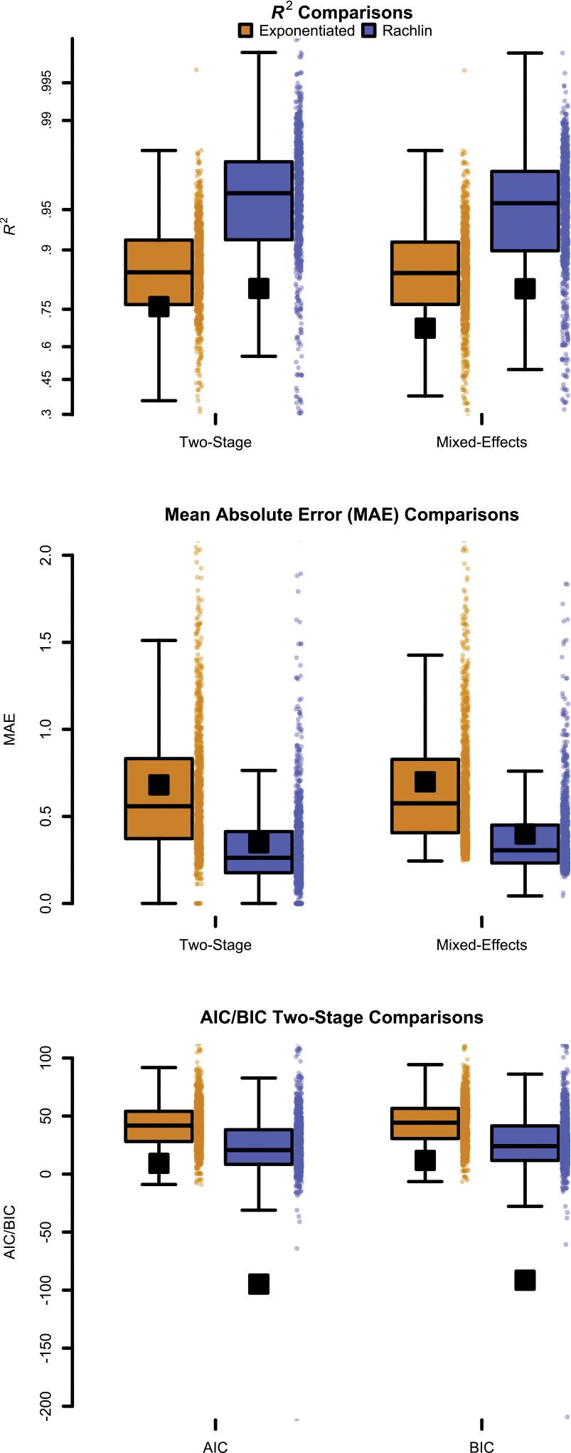
For all panels comparisons are between the exponentiated demand model (dark orange, left of pair) and the Rachlin model (blue, right of pair) from the Kaplan & Reed (2018) alcohol purchase task dataset. Top panel: Boxplots of R² from the two-stage and mixed-effects approaches for the. Horizontal black lines indicate the median, and black squares indicate the mean. Y-axis is logit-scaled to help show differences between models. Higher is better. Center Panel: Y-axis is the mean absolute error (MAE) for two-stage and mixed-effects approaches. Closer to zero is better. Bottom Panel: AIC and BIC comparisons from the two-stage models (mixed-effects model AIC/BIC values are reported in text). Lower is better for both AIC and BIC. Points to the right of a boxplot represent individual values.

Visualizations of the individual estimates from 12 select participants can be found in Figure 2. These 12 participants were chosen because they produced what might be considered “typical” purchase task demand data. Equivalent visualizations for all participants can be found in the “APT Model Comparisons” supplemental document. Generally, both models fit the data well, but the Rachlin model (blue, solid line) fit better than the exponentiated model (dark orange, dashed line). Since the Rachlin model produces better model fits and lower AIC/BIC values, it appears to potentially be a better descriptor of the processes that may have generated these data.

Figure 2.

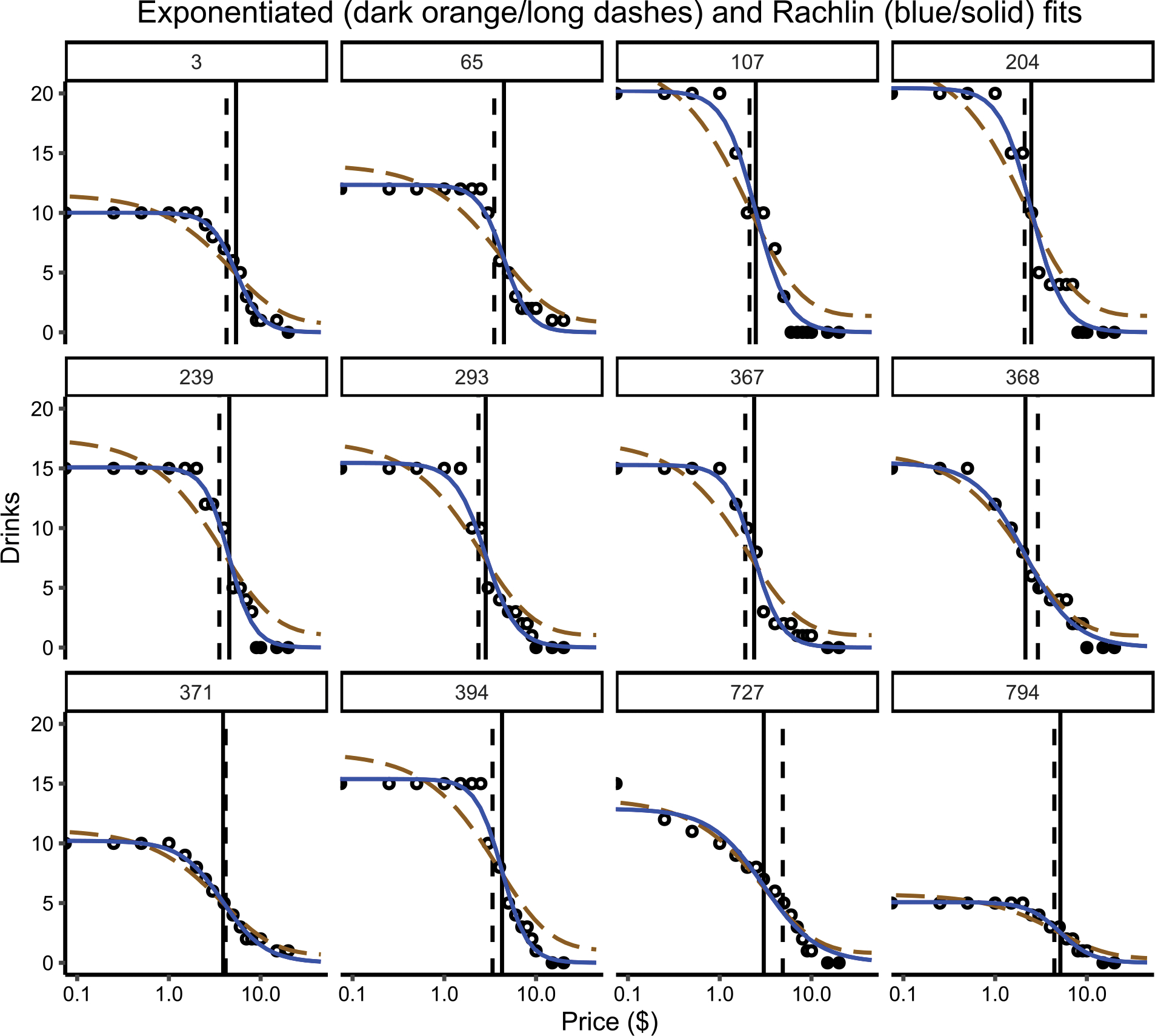
Individual model fits from the random effects from the multilevel modeling approach from the exponentiated model (dark orange, long dash) and the Rachlin model (blue, solid) to select individuals. Points that are black represent either consumption at no cost or zero consumption. P_max is indicated by the dashed vertical line, EC50 is indicated by the solid vertical line. Y-axis is number of drinks consumed, x-axis is cost per drink (log₁₀ scaled). Left-most consumption values are consumptions at zero cost, but since zeros cannot be plotted in log space, this is indicated by these points being cut in half.

P_max, O_max, EC50, and O50

To further validate Rachlin’s model on demand data, visualizations of P_max (vertical dashed lines) and EC50 (vertical solid lines) can be seen in Figure 2. Visually, EC50 corresponds with the point that the curve is at 50% of its height. For calculations of P_max there were 183 data paths (16.6%) for which Equation (4) could not be calculated with the closed solution (Equation [5]), whereas there were 0 calculation failures for EC50. These datasets all correspond to participants with estimated s parameters where s was less than 1. To calculate O_max, Equation (6) was used. Figure 3 presents the same data as Figure 2 with six participants but with consumption being multiplied by price to produce the money expended on alcohol (i.e., output or expenditure curve) and consumption with log-log scaling with a line indicating a slope of −1 at P_max. This confirms that the computations for P_max and O_max derived from Rachlin’s equation are accurate. Equivalent figures for output for all participants can be found in the “APT Output Max” supplemental document. Thus, the Rachlin model is able to furnish the traditional demand metrics P_max and O_max.

Figure 3.

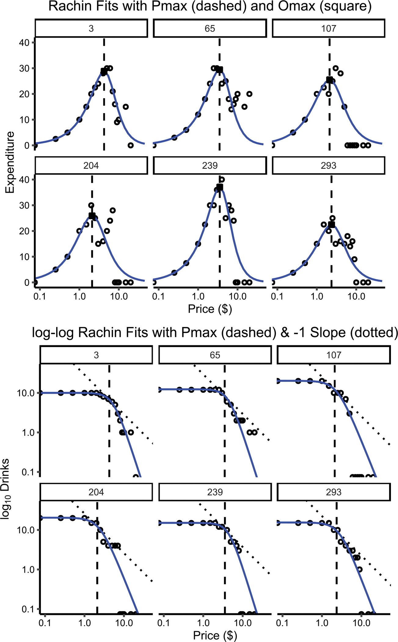
Top: Individual model fits from the random effects from the multilevel modeling approach from Rachlin model (blue, solid) to select individuals. P_max is indicated by the dashed vertical line, calculated O_max is indicated by a square. Y-axis is total expenditure on drinks (consumption * price), x-axis is cost per drink (log₁₀ scaled). Bottom: Same participants as top, but both y- and x-axes are log₁₀-scaled, with the y-axis being number of drinks consumed. Dotted line represents a slope of −1 in log-log space, dashed vertical line represents P_max. Both panels are meant to demonstrate the accuracy of the P_max derivation. Since zeros cannot be plotted in log space, this is indicated by data points that are cut in half.

Demand Metric Comparisons

Scatterplots, histograms, and correlation matrix for all various estimated parameters can be found in Figure 4. Q₀s from both models were highly correlated and resulted in nearly identical relationship with covariates. The b and s parameters for the Rachlin model were strongly correlated with each other, but displayed weaker correlations with covariates compared to α. While O50 and O_max shared a near perfect linear relationship, O_max was strongly correlated with α while O50 was not. EC50 and P_max were not related to any of the covariates.

Figure 4.

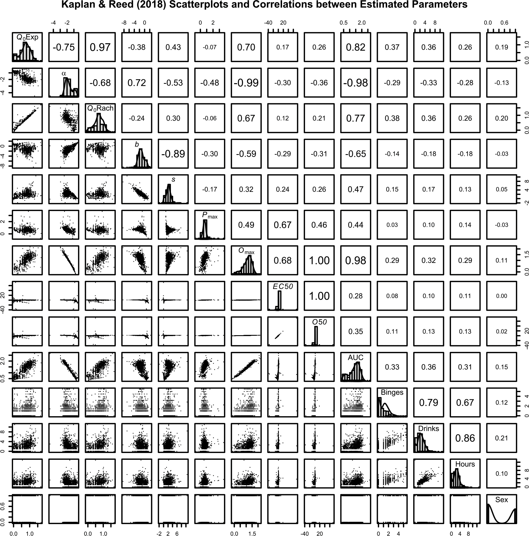
Scatterplots, histograms, and Pearson correlation matrix of estimated parameters from mixed-effects modeling versions of the exponentiated model and Rachlin model for Kaplan and Reed (2018) data. Font size is associated with strength of correlation. All parameters are log-scaled to approximate normality except demographic covariates. Binges, drinks, and hours are square root transformed to help approximate normality. Q₀Exp: Exponentiated Q₀. Q₀Rach: Rachlin Q₀. AUC: Rachlin integrated area under the curve. Binges: Number of binges. Drinks: Total number of drinks during a drinking episode. Hours: Total hours during a drinking episode. Sex: Binary coded sex variable, males were coded as 1, females were coded as 0. Correlations < .06 are not significant at the p < .05 level.

Non-Human Demand Analysis

While purchase tasks are common in research on drug demand, they are hypothetical in nature. Data from Ko et al. (2002), an animal opioid self-administration experiment, were reanalyzed from data made available in Gilroy et al. (2021)⁷ to determine how Rachlin’s equation compared to the exponentiated model for assessing consumption of a non-hypothetical commodity.

Methods

Because of the relatively small data set from Ko et al. (2002), the two-stage approach was used to fit both Equation (2) and Equation (4) to non-human primate drug demand data, rather than both the two-stage approach and mixed-effects modelling approach. Two-stage fits were determined similarly to the Alcohol Purchase Task data but starting ranges for Q₀ were adjusted for the higher levels of consumption observed. Briefly, three monkeys responded for alfentanil, remifentanil, and fentanyl at varying doses on fixed-ratio schedules of 10, 32, 100, 320, and 1000. All individual monkey data were fit for each drug at each drug dose. See Ko et al. (2002) and Gilroy et al. (2021) for more details. For the exponentiated equation, k was set to 1.669284. AUC was integrated using the Rachlin model from FRs of 0 to 1000.

Results

Fits to individual monkey data are available in Figure 5. There was only one case that the Rachlin model did not converge, which was the lowest alfentanil dose for Monkey C. For both the exponentiated and Rachlin models, mean R² was very high (.987 and .995 respectively). Both mean AIC (Exp = 37.13, Rachlin = 30.29) and BIC (Exp = 35.96, Rach = 28.73) were lower for the Rachlin model, indicating it was a more likely candidate model relative to the exponentiated model. MAE was relatively low for both the exponentiated model (MAE = 5.65) and the Rachlin model (MAE = 2.63). Scatterplots, histograms, and correlations between parameters estimated from the models can be found in Figure 6. Most results were similar to the Alcohol Purchase Task results, with the exception of O50 being strongly related to α (r = −.98). It is important to note that all three monkeys had values of s < 1 for the highest dose of fentanyl, resulting in both P_max and O_max not being calculated for those three data paths.⁸

Figure 5.

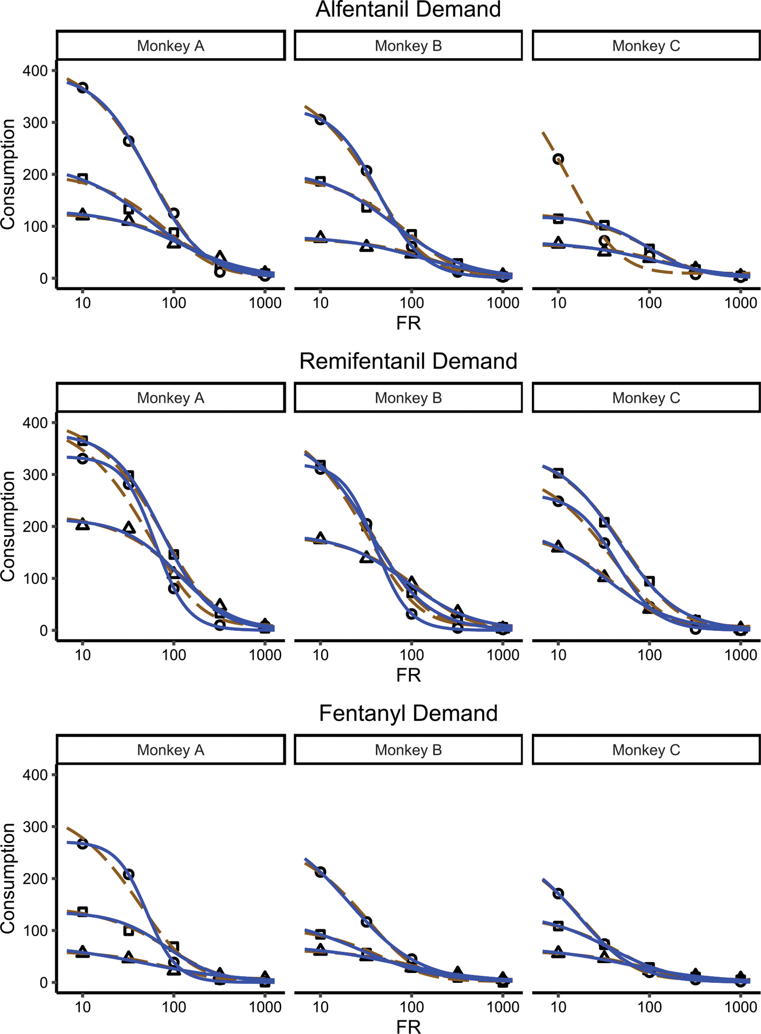
Individual model fits using the two-stage approach from the exponentiated model (dark orange, long dash) and the Rachlin model (blue, solid) to data from Ko et al. (2002). Each row is a drug, each column is a different monkey. Shapes represent different drug doses. Y-axis is doses consumed, x-axis is the fixed ratio to obtain a drug dose (FR; log₁₀ scaled). Exponentiated model fits are dark orange, long dashed, lines and the Rachlin model fits are the blue, solid, lines. Note that the Rachlin model did not converge for Monkey C for alfentanil. Circles: Lowest dose. Squares: Middle dose. Triangles: Highest dose.

Figure 6.

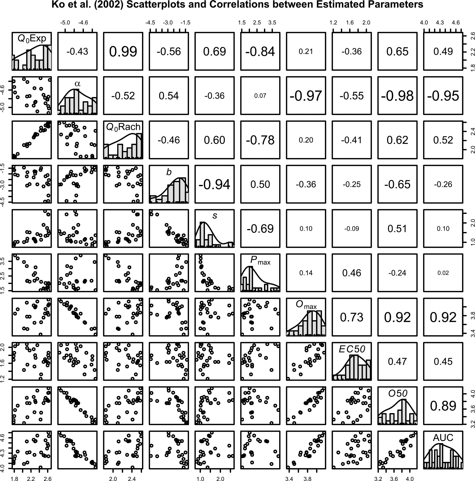
Scatterplots, histograms, and Pearson correlation matrix of estimated parameters from the two-stage approach of the exponentiated model and Rachlin model for Ko et al. (2002) data. Font size is associated with strength of correlation. All parameters are log-scaled to approximate normality. Q₀Exp: Exponentiated Q₀. Q₀Rach: Rachlin Q₀. AUC: Rachlin integrated area under the curve.

Discussion

Descriptive Fits to Data

The Rachlin model outperformed the exponentiated model for both the two-stage and mixed-effects approaches based on R², MAE, and BIC/AIC for hypothetical purchase task data and was also slightly more performant for non-human data. That is, at least in a descriptive manner, the Rachlin model appears to better describe the underlying processes for demand data in these datasets. The equations most often used in demand assume an exponential decay function, much like did early conceptualizations of decreases in value (Samuelson, 1937).⁹ Later, it was demonstrated that versions of hyperbolic decay functions better described decreases in subjective value (McKerchar & Renda, 2012; Odum, 2011; Rachlin, 2006). If demand data are also better described by a hyperbolic function, this changes some of the conceptualization of how individuals will purchase a commodity based on increased cost. The effect of increasing cost is not constant, but instead appears to decrease more sharply as prices increase. Whether the implications of this for demand are the same as discounting (e.g., preference reversals) is unclear, but conceptualizing the decrease in effort or demand hyperbolically rather than exponentially can now be empirically tested when considering cross-commodity consumption.

Conceptual Comparisons

Values of Q₀ from both models were virtually identical. This makes sense as this parameter in both models is estimating the same thing (i.e., the intercept). However, the interpretation between α from the exponentiated model and b and s from the Rachlin model is more complicated. The b and s parameters have straightforward interpretation when considering demand data, as b is the rate at which consumption decreases and s is the psychophysical perception of cost. Even though conceptually b and s might be straightforward, they are not independent of each other when considered as a measure of demand elasticity. Other derived metrics that are combinations of b and s like EC50 could address that limitation. For the exponentiated and other exponential demand equations, α is meant to represent the change in sensitivity to price but is affected by the k constant in certain equations. Conceptually, k does not relate to a theoretical property of demand, but instead is used to aid in model fitting as k and α determine the slope of the demand curve (Hursh & Silberberg, 2008). There have been attempts to rectify this issue by replacing k with Q₀ (Gilroy et al., 2021). However, due to α being partially determined by k, the same k must be used across datasets for comparisons of α to be valid. Therefore, setting k to Q₀ interferes with the ability to interpret and compare α across groups or conditions (Koffarnus et al., 2022). Replacing k with Q₀ also results in Q₀ appearing three times in the equation. Additionally, fitting values of zero with Rachlin’s equation is not a problem as the data do not need to be transformed to better accommodate the model. Although we will note that while technically the model will never predict zero, it can make predictions arbitrarily close to zero. The significance of Rachlin’s model for quantifying discounting of commodities cannot be understated. This model has time and time again been demonstrated to accurately describe the decrease in subjective value of an outcome over numerous parameters (e.g., Bruce et al., 2018; Friedel et al., 2016; Jarmolowicz et al., 2018; McKerchar et al., 2019; Sargisson & Schöner, 2020), and its extension here again appears to describe demand data as well. We must emphasize that we are not looking to necessarily replace models of exponential decay of demand data, but instead offer a new area of research on the best ways to describe demand data.

Practical Comparisons

While the ability of a model to better describe data, and the potential underlying processes therein, is important to understanding how molar and molecular decisions are made, that is only part of the value of modelling consumption data. How a model can be used practically and its relationship to other theoretically and clinically relevant outcomes are also relevant. For example, a better fitting model may not produce a parameter that correlates to clinically significant variables while a worse fitting model may. Even though there are shortfalls of existing demand models based on exponential decay, parameters estimated from them have been repeatedly shown to be related to clinically relevant outcomes (Kiselica et al., 2016; Martínez-Loredo et al., 2021; Strickland et al., 2020). On the dataset that was analyzed, α was correlated with total drinks within a week, hours of drinking a week, and binges in a week. By contrast, b and s were not as predictive of these same variables. Derived O_max was highly correlated with α, and thus was also related to the above measures. Interestingly, even though O50 and O_max were strongly correlated, O50 was not related to clinical outcomes in the same way as O_max. That is, while O_max and O50 had a .999 correlation, O_max was related to clinical outcomes (rs = ~.3) whereas O50 was less related to clinical outcomes (rs ≤ .11). Two likely explanations are that outliers may have affected the relationships, or that because EC50 occurred both above and below P_max values, resulting in O50 values that do not reflect a consistent maximum value of consumption like O_max. An additional benefit of the Rachlin model is that the metrics P_max and O_max can be derived analytically, making it easier to include those measures in future research.¹⁰ Given the high correlations between integrated AUC and α in both datasets, the utility of an AUC measure for demand seems like an interesting area to explore. Because of the relative ease of finding these values, the Rachlin equation may provide benefits in modeling over the current exponential decay versions of models of demand. Also, the s parameter may uncover interesting relationships on how individuals perceive cost, which is currently missing in the exponential models.

One of the major benefits of α in the exponential models and a large part of the conceptual justification for an exponential decay function for modeling demand data is the attractiveness of a dose-independent measure of commodity value (Hursh & Silberberg, 2008). Across a range of reinforcing doses of self-administered drug or unit size of other commodities (e.g., 1 food pellet vs. 2 food pellets), the fitted α values obtained are statistically equivalent. This is a major advantage when comparing different drugs to one another to determine which has the highest abuse liability. In the Ko et al. (2002) data reanalyzed here, three doses of three drugs were self-administered by rhesus monkeys and the fitted α values differentiated the drug being self-administered while remaining similar across doses withing a drug. The utility of this feature of demand analysis that is hard to overstate, and is not obviously shared by the fitted parameters in the Rachlin equation or other derived parameters like AUC. Therefore, even with fitting issues associated with the exponential functions, their utility may remain when comparing the value or abuse liability of qualitatively different commodities or drugs.

Other measures, such as AUC and O_max were strongly correlated with α and had similar relationships with clinical variables. This is similar to previous results comparing AUC to typical demand measures (Amlung et al., 2015; Aston et al., 2016), although AUC in the present sample was even more strongly correlated with α, possibly due to integration from the Rachlin model. This may be because the “noisiness” of observed data is removed when integrating from a fitted curve. Further research on how these different parameters from both equations relate to each other and clinical variables is still necessary. Despite some of the challenge of fitting the exponential decay function for hypothetical purchase task data, the α parameter has proven useful in explaining addiction processes. Further research will be necessary to determine if parameters derived from a hyperbolic demand model have the same practical utility. For non-human data, Rachlin’s model fit slightly better than the exponentiated, but the exponentiated still described the data extremely well (mean R² of .987). Researchers interested in applying Rachlin’s model to demand data should be aware that relationships to clinically relevant outcomes to parameters still need to be established. In the interim, we offer at least some proxies to alpha that seem to be related to clinical outcomes (e.g., integrated AUC, analytical solution for O_max), but Rachlin’s model opens an exciting area of understanding underlying processes that may best describe demand data. The exponentiated model’s parameters have the benefits of years of proven utility in correlating with addiction processes and clinical outcomes (Koffarnus & Kaplan, 2018; Martínez-Loredo et al., 2021). Because of this, further evaluations, comparisons, and relationships with other novel and well-established models of demand (see Koffarnus et al., 2022 for an overview) across species, drugs, and tasks are warranted. Because α has been predictive of actual treatment outcomes (González-Roz et al., 2020; Schwartz et al., 2021; Secades-Villa et al., 2016), future research is needed to determine how values derived from Rachlin’s equation compare to real-life outcomes, relative to established models of demand. Perhaps both models of demand could be used in tandem to address the shortfalls of one another (e.g., utility of α, ease of finding P_max/O_max).

Conclusion

At least descriptively, Rachlin’s equation that is typically used to model the rate of devaluing a commodity, more accurately described demand data than a popular exponential demand model. While parameter estimates directly derived from it did not neatly correspond with clinical outcomes (EC50, O50, b, s), other metrics from the model could (integrated AUC, O_max, Q₀). Future research should compare equations based on hyperbolic decay to established models of demand that have proved clinically useful. We do not think that it would honor Howard Rachlin’s memory to simply assume a single model’s performance on two datasets should necessitate an entire research paradigm be altered, but instead think that exploring performance of his model and its variants could help researchers better understand underlying processes related to substance use. While every question cannot be answered in relation to Rachlin’s equation and behavioral demand in the present manuscript, we believe that this opens an exciting area of research that could help inform research on substance use. Given the current results of extending his discounting model to hypothetical human and non-hypothetical non-human demand data, it appears that his notes on discounting (i.e., Rachlin, 2006) may also tentatively apply to demand.

Public Health Significance Statement:

Accurate modeling of demand data is important to quantify markers of maladaptive substance use. Howard Rachlin’s discounting equation better describes demand data than the exponentiated demand equation. Use of Rachlin’s model could allow for better quantification of patterns of maladaptive substance use and lead to a better understanding of processes in addiction.

Appendix.

Mathematical derivation of P_max

Consider the Rachlin demand equation (4)

$$Q=\frac{Q_0}{1+b{C}^s}.$$

Total expenditure is equal to consumption times cost, and can be obtained by multiplying both sides by C

$$CQ=\frac{{CQ}_0}{1+b{C}^s}.$$

The goal is to determine the value of C that maximizes total expenditure. The value of C that maximizes this function also maximizes the log of the function since the log is itself a monotone function. Thus, when searching for optima, taking the log is a common operation since it simplifies exponents to products and products to sums. Take the log of both sides.

$$\text{log}\left(CQ\right)=\log \left(C{Q}_0\right)-\text{log}\left(1+b{C}^s\right).$$

The next step requires calculus. The maximum will occur where the slope of the tangent line (i.e., the derivative with respect to C) is zero. Take the derivative and set it equal to zero

$$\frac{d}{dC}\text{log}\left(CQ\right)=\frac{1}{C}-\frac{sb{C}^{s-1}}{1+b{C}^s}=0$$

Solving the above equation for C yields P_max, the cost at which total expenditure is maximized

$$P_{max}={\left[b(s-1)\right]}^{\frac{-1}{s}}.$$

Figure 3 visually confirms this calculation for the data under analysis.

References

- Amlung M, Vedelago L, Acker J, Balodis I, & MacKillop J (2017). Steep delay discounting and addictive behavior: A meta-analysis of continuous associations. Addiction, 112(1), 51–62. 10.1111/add.13535 [DOI] [PMC free article] [PubMed] [Google Scholar]
- Amlung M, Yurasek A, McCarty KN, MacKillop J, & Murphy JG (2015). Area under the curve as a novel metric of behavioral economic demand for alcohol. Experimental and Clinical Psychopharmacology, 23(3), 168–175. 10.1037/pha0000014 [DOI] [PMC free article] [PubMed] [Google Scholar]
- Aston ER, & Cassidy RN (2019). Behavioral economic demand assessments in the addictions. Current Opinion in Psychology, 30, 42–47. 10.1016/j.copsyc.2019.01.016 [DOI] [PMC free article] [PubMed] [Google Scholar]
- Aston ER, Metrik J, Amlung M, Kahler CW, & MacKillop J (2016). Interrelationships between marijuana demand and discounting of delayed rewards: Convergence in behavioral economic methods. Drug and Alcohol Dependence, 169, 141–147. 10.1016/j.drugalcdep.2016.10.014 [DOI] [PMC free article] [PubMed] [Google Scholar]
- Bickel WK, Marsch LA, & Carroll ME (2000). Deconstructing relative reinforcing efficacy and situating the measures of pharmacological reinforcement with behavioral economics: A theoretical proposal. Psychopharmacology, 153(1), 44–56. 10.1007/s002130000589 [DOI] [PubMed] [Google Scholar]
- Borges AM, Kuang J, Milhorn H, & Yi R (2016). An alternative approach to calculating Area-Under-the-Curve (AUC) in delay discounting research. Journal of the Experimental Analysis of Behavior, 106(2), 145–155. 10.1002/jeab.219 [DOI] [PubMed] [Google Scholar]
- Bruce JM, Bruce AS, Lynch S, Thelen J, Lim S-L, Smith J, Catley D, Reed DD, & Jarmolowicz DP (2018). Probability discounting of treatment decisions in multiple sclerosis: Associations with disease knowledge, neuropsychiatric status, and adherence. Psychopharmacology, 235(11), 3303–3313. 10.1007/s00213-018-5037-y [DOI] [PubMed] [Google Scholar]
- Collins R, Parks G, & Marlatt G (1985). Social Determinants of Alcohol Consumption: The Effects of Social Interaction and Model Status on the Self-Administration of Alcohol. Journal of Consulting and Clinical Psychology, 53, 189–200. 10.1037/0022-006X.53.2.189 [DOI] [PubMed] [Google Scholar]
- Dowle M, & Srinivasan A (2020). data.table: Extension of “data.frame” (1.13.0). https://CRAN.R-project.org/package=data.table
- Franck CT, Koffarnus MN, House LL, & Bickel WK (2015). Accurate characterization of delay discounting: A multiple model approach using approximate bayesian model selection and a unified discounting measure. Journal of the Experimental Analysis of Behavior, 103(1), 218–233. 10.1002/jeab.128 [DOI] [PMC free article] [PubMed] [Google Scholar]
- Friedel JE, DeHart WB, Frye CCJ, Rung JM, & Odum AL (2016). Discounting of qualitatively different delayed health outcomes in current and never smokers. Experimental and Clinical Psychopharmacology, 24(1), 18–29. 10.1037/pha0000062 [DOI] [PMC free article] [PubMed] [Google Scholar]
- Gilroy SP, & Hantula DA (2018). Discounting model selection with area-based measures: A case for numerical integration. Journal of the Experimental Analysis of Behavior, 109(2), 433–449. 10.1002/jeab.318 [DOI] [PubMed] [Google Scholar]
- Gilroy SP, Kaplan BA, Reed DD, Hantula DA, & Hursh SR (2019). An exact solution for unit elasticity in the exponential model of operant demand. Experimental and Clinical Psychopharmacology, 27(6), 588–597. 10.1037/pha0000268 [DOI] [PubMed] [Google Scholar]
- Gilroy SP, Kaplan BA, Schwartz LP, Reed DD, & Hursh SR (2021). A zero-bounded model of operant demand. Journal of the Experimental Analysis of Behavior, 115(3), 729–746. 10.1002/jeab.679 [DOI] [PubMed] [Google Scholar]
- González-Roz A, Secades-Villa R, Weidberg S, García-Pérez Á, & Reed DD (2020). Latent Structure of the Cigarette Purchase Task Among Treatment-Seeking Smokers With Depression and Its Predictive Validity on Smoking Abstinence. Nicotine & Tobacco Research, 22(1), 74–80. 10.1093/ntr/nty236 [DOI] [PubMed] [Google Scholar]
- Hartmann MN, Hager OM, Tobler PN, & Kaiser S (2013). Parabolic discounting of monetary rewards by physical effort. Behavioural Processes, 100, 192–196. 10.1016/j.beproc.2013.09.014 [DOI] [PubMed] [Google Scholar]
- Hursh SR (1980). Economic concepts for the analysis of behavior. Journal of the Experimental Analysis of Behavior, 34(2), 219–238. 10.1901/jeab.1980.34-219 [DOI] [PMC free article] [PubMed] [Google Scholar]
- Hursh SR (1984). Behavioral economics. Journal of the Experimental Analysis of Behavior, 42(3), 435–452. 10.1901/jeab.1984.42-435 [DOI] [PMC free article] [PubMed] [Google Scholar]
- Hursh SR, & Roma PG (2013). Behavioral Economics and Empirical Public Policy. Journal of the Experimental Analysis of Behavior, 99(1), 98–124. 10.1002/jeab.7 [DOI] [PubMed] [Google Scholar]
- Hursh SR, & Silberberg A (2008). Economic demand and essential value. Psychological Review, 115(1), 186–198. 10.1037/0033-295X.115.1.186 [DOI] [PubMed] [Google Scholar]
- Jarmolowicz DP, Reed DD, Francisco AJ, Bruce JM, Lemley SM, & Bruce AS (2018). Modeling effects of risk and social distance on vaccination choice. Journal of the Experimental Analysis of Behavior, 110(1), 39–53. 10.1002/jeab.438 [DOI] [PubMed] [Google Scholar]
- Johnson MW, & Bickel WK (2008). An algorithm for identifying nonsystematic delay-discounting data. Experimental and Clinical Psychopharmacology, 16(3), 264–274. 10.1037/1064-1297.16.3.264 [DOI] [PMC free article] [PubMed] [Google Scholar]
- Kaplan BA, Foster RNS, Reed DD, Amlung M, Murphy JG, & MacKillop J (2018). Understanding alcohol motivation using the alcohol purchase task: A methodological systematic review. Drug and Alcohol Dependence, 191, 117–140. 10.1016/j.drugalcdep.2018.06.029 [DOI] [PubMed] [Google Scholar]
- Kaplan BA, Franck CT, McKee K, Gilroy SP, & Koffarnus MN (2021). Applying Mixed-Effects Modeling to Behavioral Economic Demand: An Introduction. Perspectives on Behavior Science. 10.1007/s40614-021-00299-7 [DOI] [PMC free article] [PubMed] [Google Scholar]
- Kaplan BA, Gilroy SP, Reed DD, Koffarnus MN, & Hursh SR (2019). The R package beezdemand: Behavioral Economic Easy Demand. Perspectives on Behavior Science, 42(1), 163–180. 10.1007/s40614-018-00187-7 [DOI] [PMC free article] [PubMed] [Google Scholar]
- Kaplan BA, & Reed DD (2018). Happy hour drink specials in the Alcohol Purchase Task. Experimental and Clinical Psychopharmacology, 26(2), 156–167. 10.1037/pha0000174 [DOI] [PubMed] [Google Scholar]
- Kiselica AM, Webber TA, & Bornovalova MA (2016). Validity of the alcohol purchase task: A meta-analysis. Addiction, 111(5), 806–816. 10.1111/add.13254 [DOI] [PubMed] [Google Scholar]
- Ko MC, Terner J, Hursh S, Woods JH, & Winger G (2002). Relative Reinforcing Effects of Three Opioids with Different Durations of Action. Journal of Pharmacology and Experimental Therapeutics, 301(2), 698–704. 10.1124/jpet.301.2.698 [DOI] [PubMed] [Google Scholar]
- Koffarnus MN, Franck CT, Stein JS, & Bickel WK (2015). A modified exponential behavioral economic demand model to better describe consumption data. Experimental and Clinical Psychopharmacology, 23(6), 504–512. 10.1037/pha0000045 [DOI] [PMC free article] [PubMed] [Google Scholar]
- Koffarnus MN, & Kaplan BA (2018). Clinical models of decision making in addiction. Pharmacology Biochemistry and Behavior, 164, 71–83. 10.1016/j.pbb.2017.08.010 [DOI] [PMC free article] [PubMed] [Google Scholar]
- Koffarnus MN, Kaplan BA, Franck CT, Rzeszutek MJ, & Traxler HK (2022). Behavioral economic demand modeling chronology, complexities, and considerations: Much ado about zeros. Behavioural Processes, 199, 104646. 10.1016/j.beproc.2022.104646 [DOI] [PMC free article] [PubMed] [Google Scholar]
- Locey ML, & Rachlin H (2015). Altruism and anonymity: A behavioral analysis. Behavioural Processes, 118, 71–75. 10.1016/j.beproc.2015.06.002 [DOI] [PMC free article] [PubMed] [Google Scholar]
- Malesza M (2019). The effects of potentially real and hypothetical rewards on effort discounting in a student sample. Personality and Individual Differences, 151, 108807. 10.1016/j.paid.2018.03.030 [DOI] [Google Scholar]
- Martínez-Loredo V, González-Roz A, Secades-Villa R, Fernández-Hermida JR, & MacKillop J (2021). Concurrent validity of the Alcohol Purchase Task for measuring the reinforcing efficacy of alcohol: An updated systematic review and meta-analysis. Addiction, 116(10), 2635–2650. 10.1111/add.15379 [DOI] [PMC free article] [PubMed] [Google Scholar]
- Mazur JE (1987). An adjusting procedure for studying delayed reinforcement. In The effect of delay and of intervening events on reinforcement value (pp. 55–73). Lawrence Erlbaum Associates, Inc. [Google Scholar]
- McKerchar TL, Kaplan BA, Reed DD, Suggs SA, & Franck CT (2019). Discounting Environmental Outcomes: Temporal and Probabilistic Air-Quality Gains and Losses. Behavior Analysis: Research and Practice, 19(3), 273–280. [Google Scholar]
- McKerchar TL, & Renda CR (2012). Delay and probability discounting in humans: An overview. The Psychological Record, 62(4), 817–834. 10.1007/BF03395837 [DOI] [Google Scholar]
- Mitchell SH (2004). Effects of short-term nicotine deprivation on decision-making: Delay, uncertainty and effort discounting. Nicotine & Tobacco Research, 6(5), 819–828. 10.1080/14622200412331296002 [DOI] [PubMed] [Google Scholar]
- Myerson J, Green L, & Warusawitharana M (2001). Area under the curve as a measure of discounting. Journal of the Experimental Analysis of Behavior, 76(2), 235–243. 10.1901/jeab.2001.76-235 [DOI] [PMC free article] [PubMed] [Google Scholar]
- Newman M, & Ferrario CR (2020). An improved demand curve for analysis of food or drug consumption in behavioral experiments. Psychopharmacology, 237(4), 943–955. 10.1007/s00213-020-05491-2 [DOI] [PMC free article] [PubMed] [Google Scholar]
- Odum AL (2011). Delay discounting: I’m a k, you’re a k. Journal of the Experimental Analysis of Behavior, 96(3), 427–439. 10.1901/jeab.2011.96-423 [DOI] [PMC free article] [PubMed] [Google Scholar]
- Padfield D, & Matheson G (2020). nls.multstart: Robust Non-Linear Regression using AIC Scores (1.2.0).
- Phung QH, Snider SE, Tegge AN, & Bickel WK (2019). Willing to Work But Not to Wait: Individuals with Greater Alcohol Use Disorder Show Increased Delay Discounting Across Commodities and Less Effort Discounting for Alcohol. Alcoholism: Clinical and Experimental Research, 43(5), 927–936. 10.1111/acer.13996 [DOI] [PMC free article] [PubMed] [Google Scholar]
- Pinheiro J, Bates D, DebRoy S, & Sarkar D (2020). Linear and nonlinear mixed effects models (3.1–148). https://CRAN.R-project.org/package=nlme
- R Core Team. (2022). R: A language for statistical computing (4.2.0). R Foundation for Statistical Computing. https://www.R-project.org/ [Google Scholar]
- Rachlin H (1992). Diminishing Marginal Value as Delay Discounting. Journal of the Experimental Analysis of Behavior, 57(3), 407–415. 10.1901/jeab.1992.57-407 [DOI] [PMC free article] [PubMed] [Google Scholar]
- Rachlin H (1997). Four teleological theories of addiction. Psychonomic Bulletin & Review, 4(4), 462–473. 10.3758/BF03214335 [DOI] [Google Scholar]
- Rachlin H (2006). Notes on Discounting. Journal of the Experimental Analysis of Behavior, 85(3), 425–435. 10.1901/jeab.2006.85-05 [DOI] [PMC free article] [PubMed] [Google Scholar]
- Rachlin H (2007). In what sense are addicts irrational? Drug and Alcohol Dependence, 90, S92–S99. 10.1016/j.drugalcdep.2006.07.011 [DOI] [PMC free article] [PubMed] [Google Scholar]
- Rachlin H, Green L, Kagel JH, & Battalio RC (1976). Economic Demand Theory and Psychological Studies of Choice. In Bower GH (Ed.), Psychology of Learning and Motivation (Vol. 10, pp. 129–154). Academic Press. 10.1016/S0079-7421(08)60466-1 [DOI] [Google Scholar]
- Rachlin H, & Jones BA (2008). Social discounting and delay discounting. Journal of Behavioral Decision Making, 21(1), 29–43. 10.1002/bdm.567 [DOI] [Google Scholar]
- Rachlin H, Raineri A, & Cross D (1991). Subjective probability and delay. Journal of the Experimental Analysis of Behavior, 55(2), 233–244. 10.1901/jeab.1991.55-233 [DOI] [PMC free article] [PubMed] [Google Scholar]
- Rachlin H, & Siegel E (1994). Temporal Patterning in Probabilistic Choice. Organizational Behavior and Human Decision Processes, 59(2), 161–176. 10.1006/obhd.1994.1054 [DOI] [Google Scholar]
- Reed DD, Naudé GP, Salzer AR, Peper M, Monroe-Gulick AL, Gelino BW, Harsin JD, Foster RNS, Nighbor TD, Kaplan BA, Koffarnus MN, & Higgins ST (2020). Behavioral economic measurement of cigarette demand: A descriptive review of published approaches to the cigarette purchase task. Experimental and Clinical Psychopharmacology, 28(6), 688–705. 10.1037/pha0000347 [DOI] [PMC free article] [PubMed] [Google Scholar]
- Revelle W (2020). psych: Procedures for Psychological, Psychometric, and Personality Research (2.0.8). https://CRAN.R-project.org/package=psychVersion=2.0.8
- Rodriguez ML, & Logue AW (1988). Adjusting delay to reinforcement: Comparing choice in pigeons and humans. Journal of Experimental Psychology Animal Behavior Processes, 14(1), 105–117. 10.1037/0097-7403.14.1.105 [DOI] [PubMed] [Google Scholar]
- Roma PG, Reed DD, DiGennaro Reed FD, & Hursh SR (2017). Progress of and Prospects for Hypothetical Purchase Task Questionnaires in Consumer Behavior Analysis and Public Policy. The Behavior Analyst, 40(2), 329–342. 10.1007/s40614-017-0100-2 [DOI] [PMC free article] [PubMed] [Google Scholar]
- Rzeszutek MJ, DeFulio A, & Brown HD (2022). Risk of Cancer and Cost of Surgery Outweigh Urgency and Messaging in Hypothetical Decisions to Remove Tumors. The Psychological Record, 72(3), 331–352. 10.1007/s40732-021-00489-4 [DOI] [Google Scholar]
- Rzeszutek MJ, Gipson-Reichardt CD, Kaplan BA, & Koffarnus MN (2022). Using crowdsourcing to study the differential effects of cross-drug withdrawal for cigarettes and opioids in a behavioral economic demand framework. Experimental & Clinical Psychopharmacology. 10.1037/pha0000558 [DOI] [PMC free article] [PubMed] [Google Scholar]
- Samuelson PA (1937). A Note on Measurement of Utility. The Review of Economic Studies, 4(2), 155–161. 10.2307/2967612 [DOI] [Google Scholar]
- Sargisson RJ, & Schöner BV (2020). Hyperbolic Discounting with Environmental Outcomes across Time, Space, and Probability. The Psychological Record, 70(3), 515–527. 10.1007/s40732-019-00368-z [DOI] [Google Scholar]
- Schwartz LP, Blank L, & Hursh SR (2021). Behavioral economic demand in opioid treatment: Predictive validity of hypothetical purchase tasks for heroin, cocaine, and benzodiazepines. Drug and Alcohol Dependence, 221, 108562. 10.1016/j.drugalcdep.2021.108562 [DOI] [PubMed] [Google Scholar]
- Secades-Villa R, Pericot-Valverde I, & Weidberg S (2016). Relative reinforcing efficacy of cigarettes as a predictor of smoking abstinence among treatment-seeking smokers. Psychopharmacology, 233(17), 3103–3112. 10.1007/s00213-016-4350-6 [DOI] [PubMed] [Google Scholar]
- Stein JS, Koffarnus MN, Snider SE, Quisenberry AJ, & Bickel WK (2015). Identification and Management of Nonsystematic Purchase-Task Data: Towards Best Practice. Experimental and Clinical Psychopharmacology, 23(5), 377–386. 10.1037/pha0000020 [DOI] [PMC free article] [PubMed] [Google Scholar]
- Stevens SS (1957). On the psychophysical law. Psychological Review, 64(3), 153–181. 10.1037/h0046162 [DOI] [PubMed] [Google Scholar]
- Strickland JC, Campbell EM, Lile JA, & Stoops WW (2020). Utilizing the commodity purchase task to evaluate behavioral economic demand for illicit substances: A review and meta-analysis. Addiction, 115(3), 393–406. 10.1111/add.14792 [DOI] [PubMed] [Google Scholar]
- Strickland JC, Lile JA, & Stoops WW (2017). Unique prediction of cannabis use severity and behaviors by delay discounting and behavioral economic demand. Behavioural Processes, 140, 33–40. 10.1016/j.beproc.2017.03.017 [DOI] [PMC free article] [PubMed] [Google Scholar]
- Wickham H, Averick M, Bryan J, Chang W, McGowan LD, François R, Grolemund G, Hayes A, Henry L, Hester J, Kuhn M, Pedersen TL, Miller E, Bache SM, Müller K, Ooms J, Robinson D, Seidel DP, Spinu V, … Yutani H (2019). Welcome to the Tidyverse. Journal of Open Source Software, 4(43), 1686. 10.21105/joss.01686 [DOI] [Google Scholar]
- Yoon JH, & Higgins ST (2008). Turning k on its head: Comments on use of an ED50 in delay discounting research. Drug and Alcohol Dependence, 95(1), 169–172. 10.1016/j.drugalcdep.2007.12.011 [DOI] [PMC free article] [PubMed] [Google Scholar]
- Yu J, Liu L, Collins RL, Vincent PC, & Epstein LH (2014). Analytical Problems and Suggestions in the Analysis of Behavioral Economic Demand Curves. Multivariate Behavioral Research, 49(2), 178–192. 10.1080/00273171.2013.862491 [DOI] [PubMed] [Google Scholar]
Associated Data
This section collects any data citations, data availability statements, or supplementary materials included in this article.