

Abstract
Objective:
To develop and validate a novel deep learning architecture to classify retinal vein occlusion on color fundus photographs (CFP) and reveal the image features contributing to the classification.
Methods:
The neural understanding network (NUN) is formed by two components: (a) convolutional neural network (CNN) based feature extraction and (b) graph neural networks (GNN) based feature understanding. The CNN-based image features were transformed into a graph representation to encode and visualize long-range feature interactions to identify the image regions that significantly contributed to the classification decision. A total of 7,062 CFPs were classified into three categories: (1) no vein occlusion (“normal”), (2) central retinal vein occlusion, and (3) branch retinal vein occlusion. The area under the receiver operative characteristic (ROC) curve (AUC) was used as the metric to assess the performance of the trained classification models.
Results:
The AUC, accuracy, sensitivity, and specificity for NUN to classify CFPs as normal, central occlusion, or branch occlusion were 0.975 (±0.003), 0.911 (±0.007), 0.983 (±0.010), and 0.803 (±0.005), respectively, which outperformed available classical CNN models.
Conclusion:
The NUN architecture can provide a better classification performance and a straightforward visualization of the results compared to CNNs.
Keywords: neural understanding network (NUN), retinal vein occlusion, image classification, convolutional neural network (CNN), graph neural network (GNN)
I. Introduction
Retinal vein occlusion (RVO) is the second most common retinal vascular disease [1]. If left untreated, RVO can lead to permanent vision loss [2]. Most patients develop the disease at an elderly age, and more than half of them have associated systemic disorders (e.g. hypertension, hyperlipidemia, and/or diabetes mellitus) [3]. As a type of thrombosis that affects the vasculature in the retina, RVO causes increased intravenous pressure which results in vascular tortuosity, retinal hemorrhages, cotton wool spots, and optic nerve edema. RVO can be categorized into central or branch occlusion. Central occlusion is a blockage along the main retinal vessels along the superior temporal arcade (STA) or the inferior temporal arcade (ITA). Branch occlusion is a blockage along the smaller veins in the vessel. If blockage of the retinal vein is severe, interrupted blood flow could cause a build-up and swelling of excess fluid, which may create macular edema, macular ischemia, optic neuropathy, vitreous hemorrhage, or even tractional retinal detachment [4, 5]. An acute blockage of or continuous pressure on the retinal vein may cause retina damage and ultimately lead to permanent vision loss. Clinically, CRVO can be diagnosed as either non-ischemic or ischemic based on the presentation of bleeding, venous dilation and/or tortuosity, and/or cotton wool spots [6]. Non-ischemic CRVO is more common and accounts for 80% of CRVO cases [7]. Patients diagnosed with ischemic CRVO are characterized by at least ten-disc areas of capillary non-perfusion. Furthermore, patients who develop ischemia are far more likely to develop neovascular glaucoma in the future [8]. While several therapeutic options are available [9], successful treatment requires a diagnosis immediately after symptoms develop. Fundus imaging provides an ophthalmologist with a non-invasive and efficient way to assess RVO and many ocular diseases. A standardized ocular screening program followed by an ophthalmologist’s visual inspection can provide essential information for diagnosis and treatment of RVO. Despite improvements in treatment, there remains a shortage of ophthalmologists to adequately treat patients suffering from eye-related diseases [10]. An automated algorithm that can detect RVO will be helpful for improving the early diagnosis of RVO.
A number of computerized methods have been developed to analyze medical images to detect, segment, and classify the presence of abnormalities [11–18]. Traditional machine learning approaches heavily rely on hand-crafted image features to detect abnormalities and classify images into different categories [19–21]. In contrast, convolutional neural network (CNN) approaches have demonstrated the ability to successfully classify medical images without the need to manually develop and evaluate hand-crafted image features. This is due to the ability of CNNs to automatically and progressively extract and learn thousands of image features [22, 23]. Despite the success of CNNs in image classification, only a limited number of studies were performed to analyze RVO on fundus images. Abitbol et al. [24] used CNN algorithms to classify retinal vascular diseases including RVO; however, their dataset was limited to 224 color fundus photographs (CFP) with 55 “normal” images. Nagasato et al. [25] used a dataset of 446 ultrawide-field CFPs to train a support vector machine (SVM) and deep learning model to classify branch retinal vein occlusion. In their study, the CNN-based models outperformed the SVM models. Chen et al. [26] reported that the Inception-v3 architecture [27] had the best overall performance in central and branch occlusion classification in a dataset of 8,600 CFPs. Despite CNN’s better performance compared to traditional classification methods, CNN-based classification is often limited by its “black-box” characteristic that hinders visualization and interpretation of the image features used to perform the classification [28, 29]. The class activation map (CAM) [30] leveraged convolutional layer activations to illustrate the unsupervised localization of significant image features. However, CAMs commonly fail to localize on significant regions of the image [31]. Additionally, CAM provides activation for only one layer of a CNN composed of thousands of unique activations. When convolutional feature maps are flattened prior to making a classification, it is unclear how different regions of the image interact with each other to lead to the classification decision. Being able to visualize how specific image landmarks (optic disc, fovea, STA, ITA) interact with image features related to abnormalities to form a classification decision would improve our understanding of how CNN-based models arrive at the classification.
We developed a novel deep learning architecture termed neural understanding network (NUN) to automatically classify CFPs into three categories: (1) normal, (2) branch retinal vein occlusion (BRVO), and (3) central retinal vein occlusion (CRVO). NUN uses CNN modules to extract image features and the graph neural network (GNN) to organize these features into a graph structure. NUN was designed to: (1) improve image classification by establishing “long-range” feature relationships and (2) explain the derivation of the classification results. Long-range was defined as regions that exist outside of localized kernel space and would not interact at any stage of the CNN feature extraction. We expect that when the CNN component focuses on learning features that are locally significant, the spatial interactions among these features are primarily learned by the GNN.
II. Materials and Methods
1. Study datasets
We maintain a relatively large database consisting of more than 200,000 CFPs acquired from multiple open-access datasets [32]. These CFPs were obtained using different fundus cameras (e.g., Cannon and Topcon) with a resolution ranging from 512×512 to 3849×4011. Consequently, the image quality varies significantly. Subject demographics are unavailable for most of the cases in the database. An ophthalmologist reviewed a total of 7,062 CFPs and rated 2,548 as normal, 2,188 as CRVO, and 2,326 as BRVO. We also used the STARE dataset [33], which contains 397 CFPs of patients diagnosed with 14 different diseases. Image classes were reduced to (1) CRVO, (2) BRVO, and (3) others. The dataset was split into training and validation sets at a ratio of 6:4. Approval from an ethics committee is not necessary since all images were collected from public databases. The RVO dataset along with the manual annotations is available at the link: https://github.com/cams2b/Neural-Understanding-Network.
2. Neural understanding network (NUN)
NUN is formed by two components (Fig. 1): (1) CNN-based feature extraction and (2) GNN-based feature understanding. The feature extraction component is accomplished through leveraging CNN modules to downsize the original image and encode deep feature representations of the image. Thereafter, the CNN-based features are transformed into a graph structure with a learned network topology. The image features are understood through propagating a node’s feature embedding with its local neighborhood by using graph convolution operations to distill spatially aware feature relationships. Visualizing node neighborhoods and the weighted degree matrix will provide insight into how feature embeddings interact with features in other spatial regions.
Figure 1.

The two-stage NUN architecture. Block “A”; the CNN-based feature extraction stage, which outputs the: (1) deep feature embeddings and (2) learned network topology. Block “B”; the feature understanding stage. The feature embeddings are transformed into a graph representation of the image. Edges are then pruned using the learned neighborhood topology.
GNNs were used to predict tasks at different levels of the graph (node, edge, graph) [34]. GNNs operate in non-Euclidean space, where the network topology does not exist in a predefined grid. Furthermore, GNNs can perform either network embedding or graph deep learning tasks [35]. Network embedding involves learning the network topology; creating a stable graph that could then be used to feed into traditional machine learning algorithms. Graph deep learning involves leveraging GNNs to create an end-to-end model for various tasks. GNNs used the extracted node representations to create an understanding of the graph and create predictions, which are capable of “learning” additional features for nodes through graph convolution propagation [36].
2.1. CNN-based feature extraction
We used the inception module [27] to perform feature extraction due to its ability to perform multi-scale feature extraction. Biological variability inherent in fundus images as well as the variations in equipment, operation, and ambient lighting often causes anatomical landmarks to have different feature scales. Due to latent semantic feature variability, allowing the network to extract features across multiple kernel sizes allows for the creation of generalizable features that can account for biological and imaging randomness. The benefit of creating an independent feature extraction stage is that image features are not flattened through global pooling operations. Removing global pooling allows for features to remain localized in specific regions and for improved class activation results that are interpretable to humans.
2.2. Spectral and spatial graph representation and convolutions
After passing the image through multiple inception modules, the features interact spatially once they are converted into a graphical representation of the image. A graph G was represented as , where V corresponds to the set of n nodes contained in the graph such that denotes a single node. E corresponds to the set of m edges contained in the graph and represents an edge connecting nodes vi and vj. X is a n x d node feature matrix where . An n x n adjacency matrix A describes the network’s connectivity. One corresponds to all edge connections (vi, vj) ϵ E that exist in the network. Zero corresponds to no connection between two nodes. The adjacency matrix A is a weighted adjacency matrix E to create a distinct network topology that weighs the significance of each edge connection. From the adjacency matrix A, an n*n diagonal degree matrix D was created that corresponds to each node’s degree of connection .
Graph convolution operations can be divided into two categories: spatial and spectral. Spectral convolutions use eigenvectors of the graph Laplacian to perform learning on the transformed data
| (1) |
| (2) |
where I is an identity matrix. Graph convolutional propagation was performed using the normalized Laplacian (equation 2) [37]
| (3) |
where and . W is a learnable weight matrix, and Ht−1 corresponds to the output from the previous layer in the GCN. σ corresponds to the non-linear activation function ReLU. The lack of kernel operations on local neighborhoods allows for relation-aware feature propagation; however, scalability is limited by the size of the learnable weight matrix W.
Spatial graph convolution’s use of neighborhoods closely resembles the kernel used for convolutional propagation. Unlike CNNs that operate in Euclidean space, GNNs lack a rigid topology to define node locality, making local feature extraction a topic of significant research [38]. While spectral convolutional operations perform propagation across the entire network through a series of matrix multiplications, spatial convolutions learn features on the individual nodes and node neighborhoods of a graph. Propagation occurs through an aggregation function being performed across a node’s local neighborhood. A node’s local neighborhood is not comprised of its adjacent pixels but rather by its edge connections. The aggregated features can then be passed through additional normalization operations and activation functions to generate spatial node embeddings that incorporate their neighborhood’s features. The following equation is a simplified spatial graph propagation and is used to compute the node embedding from the previous layer (equation 4) [39]
| (4) |
where and are learnable weight vectors and corresponds to the edge weight for that exists in the neighborhood of i (N(i)). are the node embeddings from the previous layer. Additionally, the aggregation function in equation 4 is a summation operation; however, mean and maximum neighborhood values were used during feature aggregation. Spatial convolutions have the benefit of being scalable due to their neighborhood aggregation and reduced computational complexity (vector operations across nodes as opposed to matrix operations across the graph). Furthermore, there is increased freedom for spatial awareness due to the inclusion of edge weights in the propagation equation.
2.3. GNN-based feature understanding
Having reduced the dimensionality of the image, each remaining encoded pixel corresponds to a node containing a feature embedding h. Initially, the graph representation of the image exists as a complete graph, where each node is directly connected to all other nodes. A learned neighborhood function that generated a sparse weighted-edge matrix for each image was used to define local topology.
(1). Learned Neighborhood Topology
The feature understanding stage of NUN is designed to take the learned feature embeddings and generate spatially aware features through aggregation relative to a node’s local neighborhood. The initial non-Euclidean conversion of our image creates a fully-connected graph representation but does not encode any spatial relativity or importance between nodes via weighted edge connections. Starting with a fully-connected network, a relevant local neighborhood must be defined through edge pruning to remove any connections that are not necessary. CNN feature maps were used as inputs to the learned neighborhood network to ensure that each image has a descriptive network topology
| (5) |
where corresponds to an element in the weighted adjacency matrix E. refers to a learned weight value for the edge connection refers to the corresponding CNN feature input and is the bias for the edge connection. σ is the non-linear activation function ReLU. The ReLU activation function was used to increase graph sparsity by dropping any edge connection with a value of 0. This process guarantees that each node has a unique local neighborhood when propagated through the graph convolution operation.
(2). Neural Understanding Graph Propagation
The initial propagation algorithm for NUN (Fig. 1) is created by combining the above-learned neighborhood (equation 5) with spatial convolution propagation (Eq. 4):
| (6) |
Abstracting the spatial aggregation algorithm further yields the equation
| (7) |
where and refer to independent activation functions, and refers to an aggregation function (add, mean, max, min) allowing for multiple variations of the propagation function based on the classification task.
The initial network is a single-path network; however, NUN was augmented to support a two-path ensemble architecture. For ensemble architectures, the CNN backbone outputs an additional flattened feature map. This feature map was then passed through a single-layer neural network before being multiplied into the vector output from the GNN.
(3). Graph visualization map (GVM)
For a classification task, it is desirable to have a mechanism that can visually and contextually explain the computer results. Class activation maps (CAMs) are widely used to explain the classification results in CNN-based approaches [40]. CAMs provide unsupervised localization through visualizing activated features from a convolutional layer. While CAMs have demonstrated localization capabilities for medical images [41], the results are unpredictable and can visualize features that are unexplainable. Graph visualization map (GVM) is a representation of various graph matrices overlaid onto their corresponding node regions of the image. Transforming vector embeddings of CNN features into a graph allows new insights into how deep learning algorithms make predictions through feature interactions. Once every node has a defined neighborhood, the weighted adjacency matrix E and the degree matrix D were used to gain insights into the significant regions of an image. While visualizing the entire adjacency matrix would be too large for human interpretation, visualizing the neighborhoods for individual nodes can explain long-range feature interactions (Fig. 2). Additionally, the degree matrix can visualize which regions of the image had the most connectivity. GVM allows the user to understand how specific regions of the image interact to create a prediction.
Figure 2.

Node neighborhood visualization. The green box represents which node’s neighborhood we are visualizing. The numbered nodes are the neighborhood of adjacent nodes that are directly connected to the current node. The node’s coloration demonstrates the strength of its edge connection.
The degree of connectivity varies greatly depending on location. In highly connected nodes, applying pruning operations improves the understanding of what regions have the highest importance in the neighborhood. To improve the visualization, thresholding operations are performed to eliminate insignificant edge connections. Before thresholding, edge connections are normalized. Information such as the average or the median number of activated nodes for a specific class can provide a new heuristic for understanding how CNNs make predictions. Figure 3 demonstrates that when a node’s neighborhood is reduced to its strongest edge connection the remaining node is centered on a bleeding region of the CFP (Fig 3.D).
Figure 3.
A: Input image. B: Initial neighborhood of direct connections for a node (green box). C: Pruned neighborhood. D: The neighbor with the strongest edge weight.
2.4. Training NUN
The CFP images were randomly split into training (n=6,339) and validation (n=723) datasets. Images were resized to 360*360-pixel resolution. Before the training, the images were preprocessed using a normalization strategy that leveraged the channel average pixel values across the dataset [42]. Average channel values were then scaled based on pixel value distributions within the image. To account for data imbalance, the minority group was oversampled to create an even distribution of classes. Additionally, geometric and intensity augmentations were performed to increase the diversity of the data.
Networks were trained for 40 epochs with a batch size of 8 images. Optimization was performed using stochastic gradient descent (SGD) with an initial learning rate of 0.001 and a momentum of 0.9. The learning rate was decreased to 0.0001 during training. All networks were implemented in PyTorch and trained on Nvidia RTX 2080 Ti. Code is available at: https://github.com/cams2b/Neural-Understanding-Network.
2.5. Performance Assessment
Three training runs for each network were performed and the average performance across the three runs was computed. Receiver operative characteristic (ROC) analysis was used to evaluate the classification performance of the NUN in assessing the presence of RVO. The area under the ROC curve (AUC) was used as the performance metric. Accuracy, sensitivity, specificity, precision, and recall were also computed. The performance of NUN was compared to ResNet [43], DenseNet [44], and Inception-v3 on the same dataset [27]. Additionally, we generated the Class activation maps (CAMs) from the Inception-v3 and NUN and compared to GVMs generated from NUN. The distribution of the number of activated nodes in the pruned degree matrix was analyzed between classes using the intersection over union (IOU) and the difference between medians (DBM) divided by overall visible spread (OVS). OVS measures the difference between the overall maximum and minimum between two distributions. A p-value less than 0.05 was considered statistically significant in all analyses.
III. Results
The NUN algorithm achieved a statistically greater accuracy of 0.911 (±0.007) for classifying CFP images as normal, CRVO, and BRVO (Table 1). The sensitivity, specificity, precision, and F1 values using NUN to classify CFPs into the three RVO categories were 0.983 (±0.010), 0.803 (±0.005), 0.881 (±0.003), and 0.911 (±0.007), respectively. The NUN also achieved micro and macro AUC values of 0.973 (±0.003) and 0.975 (±0.003), respectively, for NUN classification of CFP images into the three RVO categories, which was higher than the other classical CNN models (Table 2, Fig. 4). The AUC values differed the most in the diseased classes CRVO and BRVO with scores of 0967 (±0.006) and 0.961 (±0.010), respectively.
Table 1.
Classification performance for normal, CRVO, BRVO color fundus photographs.
| Architecture | Accuracy | Sensitivity | Specificity | Precision | F1 |
|---|---|---|---|---|---|
| ResNet | 0.889±0.007 | 0.991±0.002 | 0.756±0.013 | 0.841±0.012 | 0.888±0.008 |
| DenseNet | 0.893±0.005 | 0.988±0.008 | 0.766±0.004 | 0.850±0.003 | 0.892±0.004 |
| Inception | 0.903±0.010 | 0.981±0.003 | 0.791±0.022 | 0.872±0.017 | 0.903±0.011 |
| NUN | 0.911±0.007 | 0.983±0.010 | 0.803±0.005 | 0.881±0.003 | 0.911±0.007 |
Table 2.
AUC values for classifying normal, CRVO, BRVO color fundus photographs.
| Architecture | Micro AUC | Macro AUC | Normal AUC | CRVO AUC | BRVO AUC |
|---|---|---|---|---|---|
| ResNet | 0.974±0.002 | 0.971±0.004 | 0.999±0 | 0.965±0.003 | 0.949±0.008 |
| DenseNet | 0.971±0.006 | 0.969±0.006 | 0.998±0.002 | 0.962±0.005 | 0.946±0.012 |
| Inception-v3 | 0.972±0.006 | 0.973±0.002 | 0.996±0.001 | 0.963±0.011 | 0.958±0.003 |
| NUN | 0.973±0.003 | 0.975±0.003 | 0.994±0.006 | 0.967±0.006 | 0.961±0.010 |
Figure 4.

ROC Curves for best performing training runs of ResNet, Inception-v3, DenseNet, and Neural Understanding Network. Class 0 corresponds to normal CFPs, class 1 corresponds to CRVO, class 2 corresponds to BRVO.
There were 784 CFPs correctly and 54 incorrectly classified as “normal,” CRVO, and BRVO by both NUN and Inception v3 (Table 3). NUN and Inception-v3 uniquely classified 35 and 24 CFPs, respectively, where only one architecture correctly classified the image. Of the 78 misclassified CFPs by NUN, 66 were misclassified disease cases (i.e., BRVO instead of CRVO), and 12 cases were false negatives (or RVO classified as normal) (Table 4).
Table 3.
Classification comparison between NUN and Inception-V3.
| Measure | Count |
|---|---|
| Both Correct | 784 |
| Only NUN Correct | 35 |
| Only Inception-v3 Correct | 24 |
| Both Incorrect | 54 |
Table 4.
CFPs misclassified by NUN.
| Measure | Count |
|---|---|
| Total Incorrect | 78 |
| Abnormal case | 66 |
| Normal case | 12 |
The feature emphasis in the CAMs generated by NUN varied greatly from those generated by Inception-V3 (Fig. 5). The CAMs generated by NUN localize on diseased regions, while CAMs generated by Inception-v3 emphasize various features in the image. In a “normal” CFP without bleeding regions, the CAM produced by NUN tracked along the STA and ITA, which provided a more explainable CAM compared to the inception-V3 CAM (Fig. 5c).
Figure 5.

Classification activation maps generated from NUN (right) and generated from Inception-V3 (left) for the original CFPs (middle). The color gradient represents the degree of CNN layer activation.
The GVM displays the current node with a green square and color gradient regions for the connected regions based on the strength of the edge connection (Fig. 6). A Gaussian filter is applied to better illustrate the neighborhood. The degree of connectivity varied greatly between individual nodes. Visual interpretation demonstrates that the NUN network can incorporate not only local features but also long-range features into the GVM.
Figure 6.

Visualization of three different nodes (green square) and their connecting neighbors for four CPFs with RVO. The color gradient represents the strength of that node’s edge connection to the visualized node.
The weighted degree matrix provides useful information regarding which nodes were most emphasized across the graph (Fig. 7). Despite the entire image being passed through NUN, most of the image has little impact on prediction. The pruned degree matrix retains and highlights only the nodes with the highest degree of connectivity. Visual inspection illustrates that the nodes with the highest degree of connectivity are a combination of anatomical landmarks (optic disc, vessel, fovea, STA, ITA) as well as bleeding regions (disease biomarkers).
Figure 7.

Visualization of image (left), degree matrix (center), and pruned degree matrix (right) with a threshold of 0.75. Column 1: original images. Column 2: degree matrix. Column 3: pruned degree matrix. The color gradient represents the weighted degree matrix for the image.
The number of activated nodes in the pruned degree matrix demonstrated that the number of CFPs depicting RVO had consistently had fewer activated nodes compared to CFPs without RVO (“normal”) across three thresholds (Table 5). The number of activated nodes was consistently lower in the CFPs depicting BRVO compared to CRVO. The interquartile range for “normal” CFPs had no overlap with the CFPs depicting either BRVO or CRVO. The CFPs depicting BRVO had the most variability in node activation across the three thresholds evaluated.
Table 5.
Minimum, Q1, Median, Q3, and Maximum number of activated nodes for each class in the validation set based on different thresholds of the weighted degree matrices (n=723).
| 0.5 Threshold | Normal Fundus Image | Central Vein Occlusion | Branch Vein Occlusion |
|---|---|---|---|
| Minimum | 22 | 5 | 1 |
| Q1 | 55 | 28 | 20 |
| Median | 63 | 37 | 32 |
| Q3 | 70 | 43 | 41 |
| Maximum | 78 | 67 | 71 |
| 0.6 Threshold | Normal Fundus Image | Central Vein Occlusion | Branch Vein Occlusion |
| Minimum | 8 | 1 | 1 |
| Q1 | 35 | 15 | 9 |
| Median | 46 | 20 | 16 |
| Q3 | 53 | 27 | 26 |
| Maximum | 67 | 47 | 56 |
| 0.75 Threshold | Normal Fundus Image | Central Vein Occlusion | Branch Vein Occlusion |
| Minimum | 2 | 1 | 1 |
| Q1 | 13 | 4 | 2 |
| Median | 19 | 7 | 5 |
| Q3 | 25 | 10 | 10 |
| Maximum | 49 | 26 | 30 |
There was no intersection between the “normal” and CRVO/BRVO fundus images (Table 6). The IOUs were 0.0 between the normal and CRVO/BRVO for all three thresholds. The IOU between the CRVO and BRVO fundus images was the largest at the threshold of 0.75 with a value of 0.75. The DBM and OVS values were the largest between the normal and CRVO/BRVO fundus images.
Table 6.
IOU and distance between medians and overall visual spread values for class analysis of normal CFPs, CRVO, and BRVO.
| 0.5 Threshold | IOU | DBM/OVS |
|---|---|---|
| Normal vs. CRVO | 0 | 0.619 |
| Normal vs. BRVO | 0 | 0.62 |
| CRVO. vs. BRVO | 0.565 | 0.217 |
| 0.6 Threshold | IOU | DBM/OVS |
| Normal vs. CRVO | 0 | 0.684 |
| Normal vs. BRVO | 0 | 0.682 |
| CRVO. vs. BRVO | 0.611 | 0.222 |
| 0.75 Threshold | IOU | DBM/OVS |
| Normal vs. CRVO | 0 | 0.571 |
| Normal vs. BRVO | 0 | 0.608 |
| CRVO. vs. BRVO | 0.75 | 0.25 |
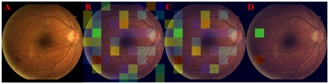
GVMs provide additional visual information for clinicians to differentiate non-ischemic CRVO from ischemic CRVO. For patients with ischemic CRVO, the GVM visualizations centered over the hemorrhaging regions of the image (Fig 8). For patients with non-ischemic CRVO, GVM visualizations split their focus between regions with bleeding and cotton wool spots (Fig 9). Figure 9A showed GVM visualization indicating isolated cotton wool regions of the retina, while Figure 9B showed GVM visualization centered on the optic disc, surrounding bleeding, and distant bleeding spots. Lack of hemorrhage in non-ischemic patients causes GVMs to be less homogenous when compared with ischemic patients. As a result, additional regions of interest (e.g., tortuous vessels and exudates) were highlighted by GVMs (Fig. 9).
Figure 8.

Highlighted regions by GVM in the fundus images acquired on two patients (A and B) diagnosed with ischemic CRVO. For both patients, the GVMs center over the optic disc with the most significant edge connections located on the surrounding hemorrhage.
Figure 9.

Highlighted regions by GVM in the fundus images acquired on two patients diagnosed with non-ischemic CRVO. For patient A, the GVM highlighted regions containing cotton wool spots. For patient B, the GVM highlighted the optic disc and surrounding bleeding spots.
The classification performance based on AUC metrics were summarized in table 7. NUN achieved micro and macro AUC values of 0.816(±0.021) and 0.873(±0.012), respectively, when evaluated on the STARE dataset. When transfer learning was used, the micro and macro AUC values were 0.900(±0.018) and 0.897(±0.021), respectively. NUN without transfer weights generated better AUCs for the classes “other” and CRVO with AUCs of 0.882(±0.019) and 0.915(±0.031), respectively. NUN with transfer weights had better performance on BRVO with an AUC of 0.934 (±0.013). Figure 10 showed the GVM-based visualizations of the regions of interest for two cases diagnosed with RVO in the STARE dataset. Visual inspection demonstrates that NUN can highlight the regions of interest associated with non-ischemic patients on general datasets.
Table 7.
Classification performance of the Neural Understanding Network (NUN) with and without transfer learning
| Architecture | Micro AUC | Macro AUC | Other AUC | CRVO AUC | BRVO AUC |
|---|---|---|---|---|---|
| NUN | 0.816(±0.021) | 0.873(±0.012) | 0.882(±0.019) | 0.915(±0.031) | 0.812(±0.066) |
| NUN w/ transfer | 0.900(±0.018) | 0.897(±0.021) | 0.849(±0.006) | 0.898(±0.057) | 0.934(0.013) |
Figure 10.

Highlighted regions by GVM in the fundus images acquired on two patients diagnosed with RVO in the STARE dataset. Patient A was diagnosed with non-ischemic CRVO, and patient B was diagnosed with BRVO. Patient A’s GVM centers on the optic disc while tracking along the tortuosity of the vessels in the retina. Patient B’s GVM tracks along the superior temporal vascular arcade and the inferior temporal vascular arcade.
IV. Discussion
We developed a novel two-stage architecture termed Neural Understanding Network (NUN) to identify RVO and classify them into different categories based on CFPs. Our objective was to improve automated RVO classification through clarifying predictions with novel visualizations and class distribution analyses. The unique characteristic of the NUN is the combination of a CNN-based feature extraction procedure and a GNN-based feature understanding (spatial interaction) procedure. The graph convolution propagation is used to organize and learn spatially aware features, ultimately improving the ability to visually interpret the features and feature interactions. The performance of the NUN was verified by classifying RVO into three categories. Rather than combining GNN features with CNN features, a single-path network was trained to create node embeddings using CNN feature extraction. Node embeddings are then used to form a non-Euclidean graph representation of the image. Neighborhood topology is encoded through a learned neighborhood network that generates each node’s locality in the graph, similar to how a kernel defines a neighborhood for an image. Once graph sparsity has been created, feature understanding occurs through graph convolutions allowing long-range feature interaction. We can gain further insight into the composition of specific classes using the learned degree matrices of the graphs.
Traditionally, a CNN architecture consists of a series of convolutional and max-pooling layers followed by a flattening of the final layer into vector space and passing the vector to a fully connected layer. While CNNs have proven incredibly capable at feature extraction, little emphasis has been placed on understanding how features interact with different spatial regions to generate a classification. Due to CNN’s reliance on kernel space for feature extraction, the creation of long-range feature connections does not occur. For CNN-based deep learning, the prediction relies on convolutional layers’ ability to recognize and extract significant features from the image. If essential biomarkers are limited or isolated to one region of the image, it is likely that they will be underrepresented when making a prediction. NUN’s establishment of a feature understanding module allows for long-range feature interactions. Isolated biomarkers can establish long-range edge connections and thus improve their feature representation during prediction. If feature representation varies during testing, edge connections can increase the feature’s degree of connectivity in the graph to improve the underlying representation. Edge pruning allows for underrepresented biomarkers to have an increased presence during machine learning feature propagation. Previous attempts to incorporate spatial attention have focused on dilated convolutions that improve spatial awareness [45]. The assumption is that increasing the kernel space would allow for the creation of spatial features. Despite these mechanisms having success, spatial features neither promote interaction across different regions of the image nor do they improve classification visualizations. GNNs have previously been used in bioinformatics applications such as drug discovery [34] and protein interactions [46]. There are only a few studies that apply GNNs to medical imaging [47–49]. Shi et al. [48] leveraged K-means clustering and the Graph Convolutional Network (GCN) to create feature representations of pathological images. The classification was performed by using the dot product to incorporate GCN features with flattened DenseNet features. While this work combined GNNs with CNNs, it did not investigate leveraging the graph to create new visualization strategies. Zhang et al. [49] leverage CNNs to extract features from fundus images prior to forming a feature graph composed of all images. Although this study used a similar framework that incorporated both CNNs and GNNs, the graph neural network’s topology is formed through each node representing one fundus image. Our graph topology is unique for each fundus image. Node feature embeddings in our graph are formed by regions within an image, rather than whole images. Our study focused on intra-image graphs while Zhang et al.’s study focused on inter-image graphs.
The main novelty of NUN is its ability to generate several GVMs of the network’s classification results that are not possible for other CNN architectures. The GVMs are made possible through matrices generated by the graph transformation of the image, namely the weighted edge connections generated by the learned network topology. While there have been several methods [38] introduced for defining a node’s local neighborhood, these approaches have been oriented towards data that already existed in non-Euclidean space, with defined edge connections. To our knowledge, this is the first study that investigated generating node neighborhoods within images.
The learned neighborhood topology allows for any region in the image to: (1) interact with different spatial areas and (2) emphasize specific regions of the image. The GVMs are capable of visualizing long-range feature interaction and emphasize an individual node’s neighborhood of connections (Fig. 6). Depending on the location of a node, as well as the features contained within the node, emphasis varied between localizing abnormal regions and identifiable landmarks that are common to CFPs (i.e., blood vessels, optic disk, macula, fovea). To our knowledge, GVMs represent the first visualization of feature interactions in a deep learning architecture. While node visualization is useful for understanding the network, the degree matrix (Figure 7) allows us to understand what regions of the network had the highest degree of connectivity and were most impactful when making a prediction or classification. For patients diagnosed with ischemic CRVO, GVM-based visualization focuses on the optic disc, with edge connections branching across the hemorrhage regions (Fig. 9). However, for patients with non-ischemic CRVO, GVMs are forced to balance their connections between small bleeding spots and other biomarkers (e.g., tortuous vessels) (Fig. 10). Visual inspection of the pruned degree matrix demonstrates that nodes containing anatomical landmarks, as well as disease biomarkers were the regions with the highest degree of connectivity. GVMs provide a unique insight into how a deep learning architecture makes a prediction.
NUN’s performance was further evaluated on the STARE dataset (Table 7). Transfer learning from our initial dataset allowed NUN to generate a micro AUC of 0.900(±0.018) and a macro AUC of 0.897(±0.021). Due to the reduced size of the dataset and 14 different types of diseases in the dataset, the training/validation split was 60/40 to largely ensure that various retinal diseases appear in each set. Although the AUC performance decreased from the initial experiments, this could be caused by the lack of sufficient images in the dataset. The example in Figure 10 demonstrated that GVMs could highlight significant regions associated with CRVO and BRVO.
While CAMs [31] can provide useful visualizations, their applicability is limited because (1) they do not show feature similarities, and (2) they do not show feature interactions. Previous attempts that used CAMs to visualize regions of interest on color fundus images confirmed that CAMs could not highlight anatomical structures associated with the classification results [50]. Also, CAMs’ performance is stable because they only highlight features that a convolutional layer highlighted [51]. In contrast, GVMs can visualize how distinct regions of the image interact with each other to form a prediction and ultimately make it possible to establish and visualize long-range feature similarities that are impossible for CAMs. GVMs rely on learned edge connections to decide which regions are the most significant rather than extracting CNN feature maps. This process allows each node autonomy to select the important region. Furthermore, clarified visualizations can help improve the development of advanced deep learning architectures through understanding feature importance.
The NUN demonstrated performance gains when compared to other CNN architectures in our cohort (Table 1). Despite being a combined dataset with large variations in image quality and resolution, the NUN was able to adapt to image variation through modeling long-range feature relationships. The ROC analysis (Fig. 4) showed that the NUN improved AUC mainly in the classification of BRVO. CAMs (Fig. 5) demonstrated that when comparing convolutional layers from identical CNNs, the features learned by the NUN improved the localization of the diseased regions.
The pruned degree matrix generated by NUN makes it possible to study the network’s node activation and thus gain insight into the underlying decisions made by the computer. We found that significantly more connected nodes were required to classify “normal” CFP compared to classifying CFPs depicting RVO abnormalities (Table 5). The increased node activation required for normal CFPs suggests that when the NUN is unable to recognize any abnormalities in the image, it applies a higher level of connectivity across all nodes in the image. When image abnormalities are detected, NUN activates fewer nodes and disregards a larger portion of the CFP. This validates our assumption that CNN architectures do not look for all regions containing image abnormalities or disease biomarkers but instead locate a sufficient number of abnormalities to reach a “threshold” to classify the image as abnormal. Through this novel heuristic GVMs generated by analyzing the degree matrix, we can hypothesize that abnormal regions in the image are being underutilized when performing classification.
The node activation between CFPs classified as BRVO and CRVO was extremely similar compared to the node activation between normal CFPs and either BRVO or CRVO CFPs (Table 6). At a threshold of 0.50, CRVO and BRVO had an interquartile IOU of 0.565, while at a threshold of 0.75, CRVO and BRVO had an IOU of 0.75. Across all thresholds, CRVO and BRVO had an IOU of 0.0 with normal CFPs. This observation was also supported by the distribution of the misclassifications (Table 4). The majority of misclassified cases were incorrect classifications between CRVO versus BRVO rather than a failure to detect RVO. There was a significant difference between the distribution of node activations between normal CFPs and either CRVO or BRVO CFPs based on DBM and OVS (Table 6). The difference between median and overall visual spread for node activations for CRVO vs. BRVO CFPs was also significantly different (DBM/OVS > 0.10). The degree matrix analysis demonstrates that we can generate novel insights about class distributions using NUN.
We are aware that the performance gains of the NUN compared to other CNN models are statistically significant (p<0.05), but still relatively small. As demonstrated by other studies [24–26], the CNN-based models were able to reasonably detect and classify the presence of RVO on CFPs, making it challenging to improve this classification performance. However, NUN can provide a better visualization of the network’s decision process based on our visual inspections, as well as provide useful analysis of the class distributions leveraging graph matrices. We believe this is a significant step beyond the existing algorithms. To more objectively assess how the NUN improves the explainability of the classification compared to other CNN-based models, a formal observer study is necessary but beyond the scope of this study. Our primary emphasis was on the computerized algorithm to identify and classify RVO into different categories. Finally, additional effort is desirable to comprehensively study how to more effectively operate the weighted edge matrix to further improve the classification performance and explainability.
V. Conclusion
We developed and validated a novel NUN architecture to classify RVO based on CFPs. To our knowledge, this is the first study that investigated graph-based node representations based on CNN feature extraction. Also, NUN allows the visualizations of how these nodes interact with each other in the image space and thus provides a new way to understand how the network makes prediction or classification decisions. Our study clearly demonstrated the level of node activation was significantly different between “normal” CFPs and CFPs depicting RVO and more similar between CFPs depicting CRVO and BRVO, which can be visualized using our graph visualization maps.
Acknowledgment
This work is supported in part by research grants from the National Institutes of Health (NIH) (R01CA237277 and R61AT012282).
References
- [1].Karia N, “Retinal vein occlusion: pathophysiology and treatment options,” Clinical opthamology, vol. 4, 2010. [DOI] [PMC free article] [PubMed] [Google Scholar]
- [2].MacDonald D, “The ABCs of RVO: a review of retinal venous occlusion,” (in eng), Clin Exp Optom, vol. 97, no. 4, pp. 311–23, Jul 2014. [DOI] [PubMed] [Google Scholar]
- [3].REHAK M and WIEDEMANN P, “Retinal vein thrombosis: pathogenesis and management,” Journal of Thrombosis and Haemostasis, vol. 8, no. 9, pp. 1886–1894, 2010. [DOI] [PubMed] [Google Scholar]
- [4].Ip M and Hendrick A, “Retinal Vein Occlusion Review,” The Asia-Pacific Journal of Ophthalmology, vol. 7, no. 1, pp. 40–45, 2018. [DOI] [PubMed] [Google Scholar]
- [5].Peter AC et al. , “Ranibizumab for Macular Edema Due to Retinal Vein Occlusions: Implication of VEGF as a Critical Stimulator,” Molecular Therapy, vol. 16, no. 4, pp. 791–799, 2008. [DOI] [PubMed] [Google Scholar]
- [6].Hayreh SS, “Classification of Central Retinal Vein Occlusion,” Ophthalmology, vol. 90, no. 5, pp. 458–474, 1983/05/01/ 1983. [DOI] [PubMed] [Google Scholar]
- [7].McIntosh RL et al. , “Natural history of central retinal vein occlusion: an evidence-based systematic review,” (in eng), Ophthalmology, vol. 117, no. 6, pp. 1113–1123.e15, Jun 2010. [DOI] [PubMed] [Google Scholar]
- [8].Chen H-F et al. , “Neovascular glaucoma after central retinal vein occlusion in pre-existing glaucoma,” BMC Ophthalmology, vol. 14, no. 1, p. 119, 2014/10/05 2014. [DOI] [PMC free article] [PubMed] [Google Scholar]
- [9].Campa C, Alivernini G, Bolletta E, Parodi BM, and Perri P, “Anti-VEGF Therapy for Retinal Vein Occlusions,” Current Drug Targets, vol. 17, no. 3, pp. 328–336, 2016. [DOI] [PubMed] [Google Scholar]
- [10].Dean WH et al. , “Ophthalmology training in sub-Saharan Africa: a scoping review,” Eye, vol. 35, no. 4, pp. 1066–1083, 2021/04/01 2021. [DOI] [PMC free article] [PubMed] [Google Scholar]
- [11].Kumar N, Narayan Das N, Gupta D, Gupta K, and Bindra J, “Efficient Automated Disease Diagnosis Using Machine Learning Models,” (in eng), J Healthc Eng, vol. 2021, p. 9983652, 2021. [DOI] [PMC free article] [PubMed] [Google Scholar]
- [12].Bakator M and Radosav D, “Deep Learning and Medical Diagnosis: A Review of Literature,” Multimodal Technologies and Interaction, vol. 2, no. 3, p. 47, 2018. [Google Scholar]
- [13].Ashraf SZ et al. , “Body composition as a Biomarker of Frailty in Patients undergoing Lobectomy,” in American Association for Thoracic Surgery Annual Meeting 2022, Boston, MA, USA, 2022. [Google Scholar]
- [14].Wang L et al. , “Feasibility assessment of infectious keratitis depicted on slit-lamp and smartphone photographs using deep learning,” International Journal of Medical Informatics, vol. 155, p. 104583, 2021/11/01/ 2021. [DOI] [PubMed] [Google Scholar]
- [15].Zhen Y, Chen H, Zhang X, Meng X, Zhang J, and Pu J, “Assessment of Central Serous Chorioretinopathy Depicted on Color Fundus Photographs Using Deep Learning,” Retina, vol. 40, no. 8, pp. 1558–1564, Aug 2020. [DOI] [PubMed] [Google Scholar]
- [16].Yu J, Yang B, Wang J, Leader J, Wilson D, and Pu J, “2D CNN versus 3D CNN for false-positive reduction in lung cancer screening,” J Med Imaging (Bellingham), vol. 7, no. 5, p. 051202, Sep 2020. [DOI] [PMC free article] [PubMed] [Google Scholar]
- [17].Wang X et al. , “Potential of deep learning in assessing pneumoconiosis depicted on digital chest radiography,” Occupational and Environmental Medicine, pp. oemed-2019-106386, 2020. [DOI] [PubMed] [Google Scholar]
- [18].Beeche C et al. , “Super U-Net: A modularized generalizable architecture,” Pattern Recognition, vol. 128, p. 108669, 2022/08/01/ 2022. [DOI] [PMC free article] [PubMed] [Google Scholar]
- [19].Ashraf SF et al. , “Predicting benign, preinvasive, and invasive lung nodules on computed tomography scans using machine learning,” J Thorac Cardiovasc Surg, Feb 16 2021. [DOI] [PubMed] [Google Scholar]
- [20].Nanni L, Ghidoni S, and Brahnam S, “Handcrafted vs. non-handcrafted features for computer vision classification,” Pattern Recognition, vol. 71, pp. 158–172, 2017/11/01/ 2017. [Google Scholar]
- [21].Cui S, Luo Y, Tseng H-H, Ten Haken RK, and El Naqa I, “Combining handcrafted features with latent variables in machine learning for prediction of radiation-induced lung damage,” Medical Physics, vol. 46, no. 5, pp. 2497–2511, 2019. [DOI] [PMC free article] [PubMed] [Google Scholar]
- [22].Mallat S, “Understanding deep convolutional networks,” Philosophical Transactions of the Royal Society A: Mathematical, Physical and Engineering Sciences, vol. 374, no. 2065, p. 20150203, 2016. [DOI] [PMC free article] [PubMed] [Google Scholar]
- [23].Wiatowski T and Bölcskei H, “A Mathematical Theory of Deep Convolutional Neural Networks for Feature Extraction,” IEEE Transactions on Information Theory, vol. 64, no. 3, pp. 1845–1866, 2018. [Google Scholar]
- [24].Abitbol E et al. , “Deep learning-based classification of retinal vascular diseases using ultra-widefield colour fundus photographs,” BMJ Open Ophthalmology, vol. 7, no. 1, p. e000924, 2022. [DOI] [PMC free article] [PubMed] [Google Scholar]
- [25].Nagasato D et al. , “Deep-learning classifier with ultrawide-field fundus ophthalmoscopy for detecting branch retinal vein occlusion,” (in eng), Int J Ophthalmol, vol. 12, no. 1, pp. 94–99, 2019. [DOI] [PMC free article] [PubMed] [Google Scholar]
- [26].Chen Q et al. , “Artificial intelligence can assist with diagnosing retinal vein occlusion,” (in eng), Int J Ophthalmol, vol. 14, no. 12, pp. 1895–1902, 2021. [DOI] [PMC free article] [PubMed] [Google Scholar]
- [27].Christian Szegedy WL, Jia Yangqing, Sermanet Pierre, Reed Scott, Anguelov Dragomir, Erhan Dumitru, Vanhoucke Vincent, Rabinovich Andrew, “Going deeper with convolutions,” 2015 IEEE Conference on Computer Vision and Pattern Recognition (CVPR), pp. 1–9, 2015. [Google Scholar]
- [28].Vellido A, “The importance of interpretability and visualization in machine learning for applications in medicine and health care,” Neural Computing and Applications, vol. 32, no. 24, pp. 18069–18083, 2020/12/01 2020. [Google Scholar]
- [29].Cabitza F, Rasoini R, and Gensini GF, “Unintended Consequences of Machine Learning in Medicine,” JAMA, vol. 318, no. 6, pp. 517–518, 2017. [DOI] [PubMed] [Google Scholar]
- [30].Zhou B, Khosla A, Lapedriza A, Oliva A, and Torralba A, “Learning Deep Features for Discriminative Localization,” 2016. [Google Scholar]
- [31].Liu H, Wang L, Nan Y, Jin F, Wang Q, and Pu J, “SDFN: Segmentation-based deep fusion network for thoracic disease classification in chest X-ray images,” Comput Med Imaging Graph, vol. 75, pp. 66–73, Jul 2019. [DOI] [PMC free article] [PubMed] [Google Scholar]
- [32].Khan SM et al. , “A global review of publicly available datasets for ophthalmological imaging: barriers to access, usability, and generalisability,” The Lancet Digital Health, vol. 3, no. 1, pp. e51–e66, 2021. [DOI] [PubMed] [Google Scholar]
- [33].Goldbaum MH, Katz NP, Nelson MR, and Haff LR, “The discrimination of similarly colored objects in computer images of the ocular fundus,” (in eng), Invest Ophthalmol Vis Sci, vol. 31, no. 4, pp. 617–23, Apr 1990. [PubMed] [Google Scholar]
- [34].Zhang XM, Liang L, Liu L, and Tang MJ, “Graph Neural Networks and Their Current Applications in Bioinformatics,” (in eng), Front Genet, vol. 12, p. 690049, 2021. [DOI] [PMC free article] [PubMed] [Google Scholar]
- [35].Wu Z, Pan S, Chen F, Long G, Zhang C, and Yu PS, “A Comprehensive Survey on Graph Neural Networks,” IEEE Transactions on Neural Networks and Learning Systems, vol. 32, no. 1, pp. 4–24, 2021. [DOI] [PubMed] [Google Scholar]
- [36].Zhou J et al. , “Graph neural networks: A review of methods and applications,” AI Open, vol. 1, pp. 57–81, 2020/01/01/ 2020. [Google Scholar]
- [37].Kipf TN and Welling M, “Semi-Supervised Classification with Graph Convolutional Networks,” p. arXiv:1609.02907 Accessed on: September 01, 2016 [Online]. Available: https://ui.adsabs.harvard.edu/abs/2016arXiv160902907K [Google Scholar]
- [38].Grover A and Leskovec J, “node2vec: Scalable Feature Learning for Networks,” presented at the Proceedings of the 22nd ACM SIGKDD International Conference on Knowledge Discovery and Data Mining, San Francisco, California, USA, 2016. [Online]. Available: 10.1145/2939672.2939754. [DOI] [PMC free article] [PubMed] [Google Scholar]
- [39].Morris C, Rattan G, and Mutzel P, “Weisfeiler and Leman go sparse: Towards scalable higher-order graph embeddings,” 2020. [Online]. Available: https://proceedings.neurips.cc/paper/2020/file/f81dee42585b3814de199b2e88757f5c-Paper.pdf.
- [40].Jung H and Oh Y, “LIFT-CAM: Towards Better Explanations for Class Activation Mapping,” ArXiv, vol. abs/2102.05228, 2021. [Google Scholar]
- [41].Kim I, Rajaraman S, and Antani S, “Visual Interpretation of Convolutional Neural Network Predictions in Classifying Medical Image Modalities,” Diagnostics, vol. 9, no. 2, p. 38, 2019. [DOI] [PMC free article] [PubMed] [Google Scholar]
- [42].Zhen Y, Wang L, Liu H, Zhang J, and Pu J, “Performance assessment of the deep learning technologies in grading glaucoma severity,” ArXiv, vol. abs/1810.13376, 2018. [Google Scholar]
- [43].Kaiming He XZ, Ren Shaoqing, Sun Jian, “Deep Residual Learning for Image Recognition,” IEEE Conference on Computer Vision and Pattern Recognition (CVPR), pp. 770–778, 2016. [Google Scholar]
- [44].Huang G, Liu Z, Van Der Maaten L, and Weinberger KQ, “Densely Connected Convolutional Networks,” 2017. [Google Scholar]
- [45].Liang-Chieh Chen GP, Schroff Florian, Adam Hartwig, “Rethinking Atrous Convolution for Semantic Image Segmentation,” ArXiv, 2017. [Google Scholar]
- [46].Chen M, Wei Z, Huang Z, Ding B, and Li Y, “Simple and Deep Graph Convolutional Networks,” presented at the Proceedings of the 37th International Conference on Machine Learning, Proceedings of Machine Learning Research, 2020. [Online]. Available: https://proceedings.mlr.press/v119/chen20v.html. [Google Scholar]
- [47].Adnan M, Kalra S, and Tizhoosh H, “Representation Learning of Histopathology Images using Graph Neural Networks,” 04 2020. [Google Scholar]
- [48].Shi J, Wang R, Zheng Y, Jiang Z, Zhang H, and Yu L, “Cervical cell classification with graph convolutional network,” (in eng), Comput Methods Programs Biomed, vol. 198, p. 105807, Jan 2021. [DOI] [PubMed] [Google Scholar]
- [49].Zhang G et al. , “Hybrid Graph Convolutional Network for Semi-Supervised Retinal Image Classification,” IEEE Access, vol. 9, pp. 35778–35789, 2021. [Google Scholar]
- [50].Yoo TK, Ryu IH, Kim JK, Lee IS, and Kim HK, “A deep learning approach for detection of shallow anterior chamber depth based on the hidden features of fundus photographs,” Computer Methods and Programs in Biomedicine, vol. 219, p. 106735, 2022/06/01/ 2022. [DOI] [PubMed] [Google Scholar]
- [51].Chen C, Li O, Tao D, Barnett A, Rudin C, and Su JK, “This Looks Like That: Deep Learning for Interpretable Image Recognition,” 2019. [Online]. Available: https://proceedings.neurips.cc/paper/2019/file/adf7ee2dcf142b0e11888e72b43fcb75-Paper.pdf.