Fuzzy-based prediction of solar PV and wind power generation for microgrid modeling using particle swarm optimization

Abstract

Regardless of their nature of stochasticity and uncertain nature, wind and solar resources are the most abundant energy resources used in the development of microgrid systems. In microgrid systems and distribution networks, the uncertain nature of both solar and wind resources results in power quality and system stability issues. The randomization behavior of solar and wind energy resources is controlled through the precise development of a power prediction model. Fuzzy-based solar PV and wind prediction models may more efficiently manage this randomness and uncertain character. However, this method has several drawbacks, it has limited performance when the volumes of wind and solar resources historical data are huge in size and it has also many membership functions of the fuzzy input and output variables as well as multiple fuzzy rules available. The hybrid Fuzzy-PSO intelligent prediction approach improves the fuzzy system's limitations and hence increases the prediction model's performance. The Fuzzy-PSO hybrid forecast model is developed using MATLAB programming of the particle swarm optimization (PSO) algorithm with the help of the global optimization toolbox. In this paper, an error correction factor (ECF) is considered a new fuzzy input variable. It depends on the validation and forecasted data values of both wind and solar prediction models to improve the accuracy of the prediction model. The impact of ECF is observed in fuzzy, Fuzzy-PSO, and Fuzzy-GA wind and solar PV power forecasting models. The hybrid Fuzzy-PSO prediction model of wind and solar power generation has a high degree of accuracy compared to the Fuzzy and Fuzzy-GA forecasting models.

The rest of this paper is organized as: Section II is about the analysis of solar and wind resources row data. The Fuzzy-PSO prediction model problem formulation is covered in Section III. Section IV, is about the results and discussion of the study. Section V contains the conclusion. The references and abbreviations are presented at the end of the paper.

1. Introduction

Wind and solar resources are the most plentiful renewable energy resources and will dominate the world'smajority of green power generation soon. The main challenge in utilizing these resources is their volatile nature. The availability of both solar and wind resources varies from time to time, and they have an indeterministic nature. This uncertain characteristic will cause system planning, system stability and security, maintenance scheduling, and power quality issues [1]. Therefore, a precise forecast of both solar and wind-based power generation is one of the solutions to reduce its intermittency. This will mitigate the above-mentioned power system issues that exist during the integration of wind and solar PV generators into the power system network [2]. In the last ten years, various types of research have been carried out on the prediction of solar and wind power generation, including some statistical models like ARMA, ARIMA, and intelligent renewable energy prediction models like Fuzzy, Fuzzy-PSO, ANFIS, ARIMA-ANN, etc. [[3], [4], [5], [6], [7], [8]]. The intelligent solar and wind prediction models are categorized as hybrid and stand-alone approaches. The stand-alone prediction approach consists of a single intelligent prediction technique such as a fuzzy model, a support vector machine model, or an ANN. On the other hand, the hybrid approach includes one or more intelligent or statistical prediction techniques combined with another prediction approach to enhance the weakness of the individual prediction models. Some hybrid renewable power generation prediction models are wavelet-ANFIS-PSO, ARMA-ANN, ARIMA-SVR, etc. [[9], [10], [11]]. However, all the prediction approaches mentioned above are based on weather-based forecasts, whereas the proposed prediction approach in this paper also introduces a new input variable called the ECF in addition to the weather parameters that improve the forecast accuracy.

The fuzzy-based solar irradiance forecast model takes into account the previous day's meteorological and solar radiation measurements, which are then optimized using the fuzzy c-mean clustering algorithm and simulated annealing [12]. The subtractive clustering technique is used by the model based on the fuzzy c-mean clustering method to generate the fuzzy rules from the prediction dataset. They also developed a second model based on fuzzy c-mean clustering and a simulated annealing algorithm to improve the accuracy of the fuzzy logic system. The results of the proposed model demonstrate that the root-mean-square error (RMSE) for the second model modified by simulated annealing was roughly 88%, compared to 79.75% accuracy for the first model.

Furthermore, in other literature, various weather variables have also been considered. Climatic data like as solar radiation, wind speed, precipitation, and temperature are used in short-term solar power forecasts based on solar PV power and weather data obtained from 182 sites [13]. The authors, in Ref. [13] proposed deep learning and ANN as a training technique for accurate forecasting of solar PV power. In this paper, the goal of the forecast is to maintain the stability of solar power generation while the validity of the proposed approach is evaluated using the root-mean-square error (RMSE), mean absolute percentage error (MAPE), and normalized root-mean-square error (NRMSE). This methodology demonstrated the best forecast has an RMSE of 8.768.

In [14], a short-term solar power forecast using a novel hybrid approach called the Mycielski-Markov method has been introduced. This new hybrid approach is developed using two different methods; the Mycielski and the Markov chain technique. The Mycielski approach of identifying the data trend and correlation that determines the recurring of the solar radiation data. It deterministically forecasts future data patterns based on their recurrence. The Markov approach, on the other hand, generates transition probabilities for solar energy levels and forecasts states based on these probabilities. The findings of the hybrid Mycielski-Markov solar power generation forecast model have a very low forecasting accuracy whose MAPE is 30.64% while the RMSE is 32.65. A solar prediction approach based on a support vector machine (SVM) with reliable data has been developed [15] to decrease prediction error. To construct the training samples, comparable datasets were identified from the obtained historical datasets using a pattern recognition algorithm with Euclidean distance. Applying a wavelet decomposition and developing a different SVM solar power generation forecast model using a similar day training dataset yields an RMSE error of 19.05% [16]. presents a unique approach for estimating 24-h sun radiation using predefined artificial neural networks. The historical daily weather data obtained from the solar PV system location was utilized to supplement the standard artificial neural networks approach. The ANN-based solar PV power generation prediction model produces good forecasting results with low prediction errors.

A wind power prediction model using a least-square support vector machine (LSSVM) has been developed by Ref. [17]. According to this model, the performance of the LSSVM in predicting wind power generation is depending on the accuracy of selecting the parameters of the LSSVM. The authors introduce a fruit fly optimization algorithm (FOA) to avoid human-made errors in choosing the parameters of the LSSVM. The performance of the FOA-LSSVM wind power generation forecast model is compared with the LSSVM and LSSVM-PSO. The FOA-LSSVM wind power generation prediction model has a good prediction RMSE accuracy of 14.23% while that of the LSSVM has an accuracy of 19.14% and the LSSVM-PSO has an accuracy of 17.59%. In Ref. [18], the convolutional neural network (CNN) and genetic algorithm (GA) based wind power generation forecast for a large wind farm is proposed to handle the forecasting error, which is caused by both inherent stochastic factors and extrinsic stochastic factors. The performance of the CNN-GA model is compared to the GA alone and the backpropagation neural network (BPNN). It has a relatively good prediction RMSE accuracy of 14.3% as compared to GA with 16.15% and BPNN alone with 14.62%.

The estimation of wind and solar power generation based on a modified fuzzy prediction interval using fuzzyregression (FR), firefly algorithm (FF), cultural algorithm (CA), genetic algorithm, and particle swarm optimization is developed in Ref. [19]. According to this model, for a short prediction interval (less than 1 day), the GA-based fuzzy prediction model provides a better prediction accuracy (RMSE of 1.88), whereas, for a longer prediction interval (>1day), the PSO-based fuzzy prediction model has better performance (RMSE of 7.5) [19]. For one-day-ahead hourly solar PV [20] and short-term wind power prediction [21], a hybrid solution based on a mix of PSO, ANFIS, and genetic algorithms is presented. The proposed method is compared to two additional prediction methods: persistence and back propagation neural network (BP-NN) [20]. The model has been evaluated on several solar PV systems, and the new PSO-ANFIS prediction model outperforms both the BP-NN and Persistence methods. Table 1 highlights the performance of the various solar PV and wind power prediction methods and serves as a baseline for evaluating the performance of the model mentioned in this study.

Table 1.

Selected wind and solar PV power prediction models summary table.

No.	Paper Title	Model	System	RMSE	MAPE	Reference
1.	Short-Term Solar Power Forecasts Considering Various Weather Variables	Deep Learning and ANN	Solar PV	8.768	–	[13]
2.	Short-Term Solar Power Generation Forecasting: A Novel Approach	Mycielski signal processing and probabilistic Markov chain technique	Solar PV	32.65	30.64	[14]
3.	Short-term solar radiation prediction based on SVM with similar data	support vector machine, SVM	Solar PV	19.05	–	[15]
4.	Wind Power Day-ahead Prediction Based on LSSVM With Fruit Fly Optimization Algorithm,	FOA-LSSVM	Wind	14.23	–	[17]
		LSSVM-PSO		17.59	–
		LSSVM		19. 17	–
5.	Research on Wind Power Prediction Method Based on Convolutional Neural Network and Genetic Algorithm	CNN-GA	Wind	14.3	–	[18]
		GA		16.15	–
		BPNN		14.62	–
6.	Renewable Generation (Wind/Solar) and Load Modeling through Modified Fuzzy Prediction Interval	FR	Solar PV Wind	8.52	8.91	[19]
		CA		39.5	26.78
		FF		9.42	8.94
		GA		10.19	8.35
		PSO		7.5	9.8
7.	PSO-ANFIS-based Hybrid Approach for Short-Term PV Power Prediction in Microgrids	PSO-ANFIS	Solar PV	6.82	3.47	[20]
		BP-NN		9.17	4.78
		Persistence		11.32	6.26
8.	Short-Term Wind Power Prediction in Microgrids using a Hybrid Approach Integrating GA, PSO, and ANFIS	GA-PSO-ANFIS	Wind	–	6.79	[21]
		I. NF		–	6.92
		II. GA-BP NN		–	7.03
		III. BP NN		–	7.07

2. Solar and wind resources data analysis

The precision of wind and solar power generation forecasting is determined by both intrinsic and external stochastic variables. The inherent stochastic factor is related to the model parameter and methodology, whereas the extrinsic stochastic factor is associated with the model data inputs. From the past research article, the inherent factors are the heart of the wind and solar power generation forecasting models, which accounts for the critical extrinsic stochastic input parameters. That is why the temperature, time, ECF, historical irradiance, and wind speed information in this paper is considered extrinsic input parameter. This approach also reduces the computational time of the prediction model for a large iteration number of PSO. The MATLAB/Simulink simulation software is used to model both the Fuzzy and Fuzzy-PSO predictive algorithms. An accurate forecast model of wind and solar power requires testing and training datasets. The training and testing datasets of solar radiation, wind speed, and weather information have been collected from the National Metrology Agency of Ethiopia. The hourly normal and diffused solar irradiances, wind speed, and temperature data have been collected from 2017 to 2019/20 and analyzed for the Fuzzy-PSO solar PV and wind power prediction models. The Fuzzy-PSO models are trained using 17,520 hourly data in 2017 and 2018, while the 2019/20 wind and solar data are used to verify the Fuzzy-PSO power prediction models of the wind and solar systems, respectively.

2.1. Solar PV power

The output of the solar PV power plant depends on the PV efficiency, the global horizontal irradiance (GHI), and the atmospheric temperature [22]. The GHI can be computed using the DNI (direct normal insolation), DSI (diffused solar insolation), and considering the solar zenith angle (sza) [19].

$$\mathrm{G}\mathrm{H}\mathrm{I}=\mathrm{D}\mathrm{N}\mathrm{I}.\cos \left(\mathrm{s}\mathrm{z}\mathrm{a}\right)+\mathrm{D}\mathrm{S}\mathrm{I}$$ (1)

The solar power output is estimated using the data in Eq. (1), the temperature coefficients of the PV cell, the ambient temperature, and cell efficiency.

$${\mathrm{P}}_{\mathrm{p}\mathrm{v}}={\eta .\mathrm{A}}_{\mathrm{p}\mathrm{v}}.\mathrm{G}\mathrm{H}\mathrm{I}\left(\mathrm{t}\right)\left[1+\left(\alpha -\beta \right).\Delta \mathrm{T}\right]$$ (2)

where, $\eta$ is the efficiency of the PV cell (15%), ${\mathrm{A}}_{\mathrm{p}\mathrm{v}}$ is the size of the PV panel, α = 20e-6A/^oc and β = 5e-3V/^oc are the temperature coefficient of current and voltage respectively, $\Delta \mathrm{T}=\left({\mathrm{T}}_{\mathrm{a}\mathrm{c}}-{\mathrm{T}}_{\mathrm{s}\mathrm{t}\mathrm{c}}\right)$ is the temperature deviation of the PV module.

The value of α and β depends on the insolation level and the types of PV cell material, and it should be converted into percentage per degree cent grade (%/^oc) using the standard values of an open circuit voltage, Voc = 720 mV (β = 0.69%/^oc), and a short circuit current, I_sc = 350A/m² (α = 0.057%/^oc) to compute the solar PV power using Eq. (2) [23].

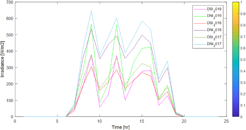
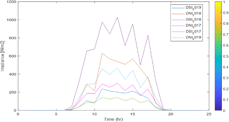
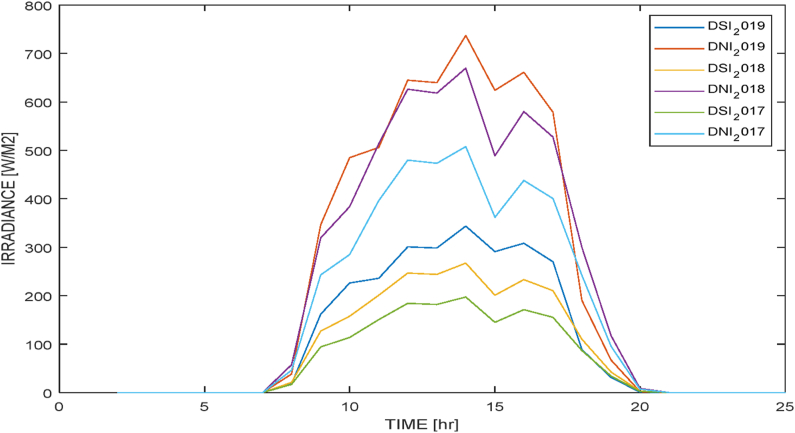
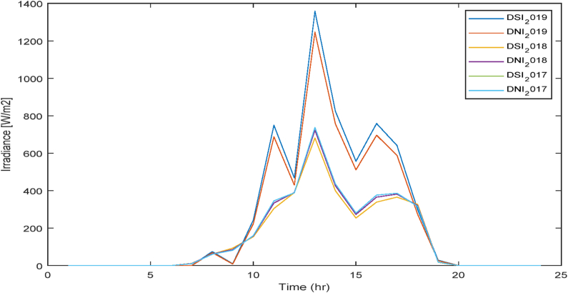
The three-year hourly average DNI and DSI solar resource data on a seasonal basis are presented in Figs. 1–4. The seasonal average daily solar PV power density profile and the yearly average daily solar PV power density profiles are computed using Eq. (2). The information in Figs. Fig. 1, Fig. 2, Fig. 3, Fig. 4 are utilized to learn and verify a fuzzy prediction model of solar power generation using PSO.

Fig. 1.

Fall season hourly average DNI and DSI profile.

Fig. 2.

Winter season hourly average DNI and DSI profile.

Fig. 3.

Spring season hourly average DNI and DSI profile.

Fig. 4.

Summer season hourly DNI and DSI profile.

2.2. Wind power

The wind generator's power output depends on the height of the turbine, the electromechanical conversion efficiency, the wind speed, the air density, and the area swept by the turbine blade [24].

Eq. (3) expresses the link between wind speed and turbine height.

$${\mathrm{V}}_2={\mathrm{V}}_1{\left(\frac{{\mathrm{Z}}_2}{{\mathrm{Z}}_1}\right)}^{\mathrm{a}}$$ (3)

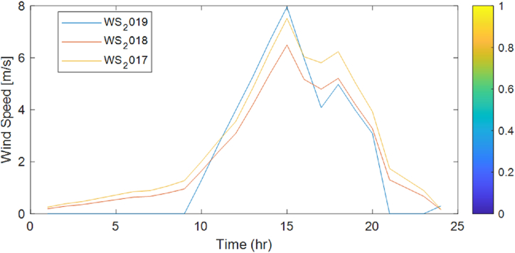
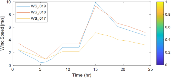
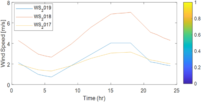
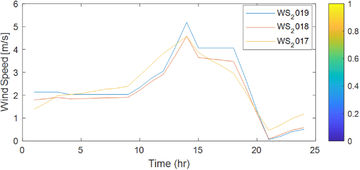
where, v₁ is the initial wind speed measurement at a height of z₁, v₂ is the transformed wind speed at the turbine height, z₂ and a (0.25 for cities containing tall buildings) is a shear exponent that measure the surface roughness of the terrain. Fig. 5, Fig. 6, Fig. 7, Fig. 8 show the three-years wind speed data at 50 m above the ground on a seasonal basis.

Fig. 5.

Fall season hourly average wind speed profile @50 m.

Fig. 6.

Winter hourly average wind speed profile @50 m.

Fig. 7.

Spring season hourly average wind speed profile @50 m.

Fig. 8.

Summer season hourly average wind speed profile @50 m.

The estimated wind generator power from the information given in Eq0.3 and the wind conversion coefficient (Cp) and turbine blade swept area (${\mathrm{A}}_{\mathrm{s}\mathrm{w}}$) is given in Eq. 4. Albert Betz discovered that by whirling a rotor, no wind turbine can transform more than 59.3% of the wind's kinetic energy into mechanical energy. This is known as the Betz Limit, and it represents the theoretical maximum power efficiency of any wind turbine. This variable is used to compute wind power [25].

$${\mathrm{P}}_{\mathrm{w}}=\frac{1}{2}\rho *{\mathrm{A}}_{\mathrm{s}\mathrm{w}}*{\mathrm{C}}_{\mathrm{p}}\left(\gamma ,\beta \right)*{\mathrm{V}}^3$$ (4)

where, $\rho$ is the density of air (1.225 kg/m3), $\gamma$ is the tip speed ratio determined by the linear speed of the wind and the rotational speed of the rotor, and $\beta$ is the pitch angle.

3. The fuzzy-PSO model problem formulation

3.1. Fuzzy system

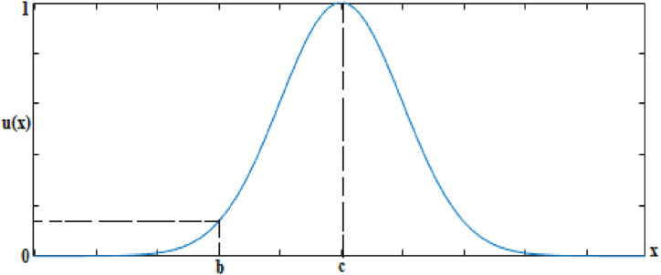
For the solar power prediction model, the fuzzy logic system has four fuzzy input variables: time, temperature, ECF, and previous solar power. However, the wind power prediction model has three input fuzzy variables: time, ECF, and previous wind power. The predicted solar PV and wind power results are the only output fuzzy variables of both models. Since the Gaussian membership function, $u\left(x\right)$-in Eq. (5), is the most effective and well-defined representation of most real-world problems and it is considered for this study. The representation of the Gaussian membership function is defined using two fundamental parameters (mean, c and standard deviation, b) as shown in Fig. 9.

$$u\left(x,b,c\right)=e^{\frac{{-\left(x-c\right)}^2}{2b^2}}$$ (5)

Fig. 9.

The Gaussian fuzzy membership function.

In this research, a novel fuzzy input variable is introduced in the Fuzzy-PSO wind and solar power forecasting models to improve the forecasting accuracy. This variable is called the error correction factor (ECF), and it was computed from the initial fuzzy prediction model of time series forecast result and validation data set using Eq. (6). It is used to pre-adjust the behavior of the prediction, which is based on the fuzzy-alone information that has been done before tuning the model using PSO. The Fuzzy-PSO forecasting model can intelligently generate the rules and membership functions of the fuzzy system using the input-output training dataset pairs. The three-year hourly dataset of solar and wind resources has been collected from the National Metrology Agency of Ethiopia and a short-term daily forecast of solar and wind power generation on a 24-hourly basis is conducted based on the seasonal and the overall annual average historical datasets. The accuracy level of the newly developed Fuzzy-PSO solar PV and wind power prediction model is compared to the fuzzy-alone, Fuzzy-GA without ECF, and the different solar PV and wind power prediction models developed in the literature. An ECF introduced in this paper has greatly enhanced the performance of the prediction models and is defined in Eq. (6).

$$\mathrm{E}\mathrm{C}\mathrm{F}=\frac{{\mathrm{F}}_{\mathrm{A}}-{\mathrm{F}}_{\mathrm{F}}}{{\mathrm{F}}_{\mathrm{A}}}$$ (6)

where, F_A is the actual (validation) solar PV or wind power dataset, and F_F is the corresponding forecasted dataset.

The value of ECF is considered as a guide for fuzzy rule generation and helps to easily understand the correlation between the input and output fuzzy variables. Negative values of the ECF indicate the forecasted dataset values are greater than the validation dataset values, whereas the positive valves of ECF indicate the validation dataset is greater than the forecasted dataset values. Therefore, when the ECF is positive, the fuzzy rules and the fuzzy input and output variables correlation should be revised to increase the forecasted dataset values and minimize the values of the error measurement. On the other hand, when the ECF is negative, the fuzzy rules and the fuzzy input and output variables correlation should be adjusted in such a way that to decrease the forecasted dataset values and minimize the values of the error measurement to zero.

3.2. Particle swarm optimization

Kennedy and Eberhart proposed PSO in 1995 [26], which is basically the intelligence of birds flocking or schooling of fish. However, Shi and Eberhart improved the original PSO in 1999 [27] to enhance the premature convergence and degree of precision given the inertia weight factor, ω. It was a six-step iterative process to get the optimal solution of the fuzzy rules and membership functions. PSO is selected over the other heuristic optimization algorithm because of its superior performance to search both local and global optimal points and provides better solutions; fast convergence rate and ease to program. In addition, its simplicity to manage premature convergence is also made PSO a preferred optimization algorithm by most researchers.

PSO algorithm steps: 28

• i.Initialization of PSO coefficients [r₁, r_2, ω, c₁, c₂].
• ii.Generation of the initial solution randomly in the search space domain. From the fitness function of the initial solution, the particles position and velocity are evaluated to identify the personal best and global best values.
• iii.Use Eqs. (7) and (8) to update the particles position and velocity.

$${\mathrm{V}}_{\mathrm{i}\mathrm{d}}^{\mathrm{t}+1}=\omega .{\mathrm{V}}_{\mathrm{i}\mathrm{d}}^{\mathrm{t}}+{\mathrm{c}}_1{\mathrm{r}}_1\left({\mathrm{P}}_{\mathrm{i}\mathrm{d}}^{\mathrm{t}}-{\mathrm{x}}_{\mathrm{i}\mathrm{d}}^{\mathrm{t}}\right)+{\mathrm{c}}_2{\mathrm{r}}_2\left({\mathrm{G}}_{\mathrm{d}}^{\mathrm{t}}-{\mathrm{x}}_{\mathrm{i}\mathrm{d}}^{\mathrm{t}}\right)$$ (7)

$${\mathrm{x}}_{\mathrm{i}\mathrm{d}}^{\mathrm{t}+1}={\mathrm{x}}_{\mathrm{i}\mathrm{d}}^{\mathrm{t}}+{\mathrm{V}}_{\mathrm{i}\mathrm{d}}^{\mathrm{t}+1}$$ (8)

iv. Using Eq. (9), the inertia weight factor is also adjusted at every iteration.

$${\omega }^{\mathrm{t}+1}={\omega }_{\max }-\frac{\left({\omega }_{\max }-{\omega }_{\min }\right)\times \mathrm{c}\mathrm{u}\mathrm{r}\mathrm{r}\mathrm{e}\mathrm{n}\mathrm{t}\mathrm{i}\mathrm{t}\mathrm{e}\mathrm{r}\mathrm{a}\mathrm{t}\mathrm{i}\mathrm{o}\mathrm{n}}{\mathrm{m}\mathrm{a}\mathrm{x}\mathrm{i}\mathrm{m}\mathrm{u}\mathrm{m}\mathrm{i}\mathrm{t}\mathrm{e}\mathrm{r}\mathrm{a}\mathrm{t}\mathrm{i}\mathrm{o}\mathrm{n}}$$ (9)

• v.At each iteration, the particle's personal best and global best positions should be updated.

$${\mathrm{P}}_{\mathrm{i}\mathrm{d}}^{\mathrm{t}+1}={\mathrm{x}}_{\mathrm{i}\mathrm{d}}^{\mathrm{t}+1}\mathrm{i}\mathrm{f}\mathrm{f}\left[{\mathrm{X}}_{\mathrm{k}}\left(\mathrm{t}+1\right)\right]\le \mathrm{f}\left[{\mathrm{P}}_{\mathrm{k}}^{\mathrm{b}}\left(\mathrm{t}\right)\right]$$ (10)

$${\mathrm{G}}_{\mathrm{k}}^{\mathrm{b}}\left(\mathrm{t}+1\right)={\mathrm{X}}_{\mathrm{k}}\left(\mathrm{t}+1\right)\mathrm{i}\mathrm{f}\mathrm{f}\left[{\mathrm{X}}_{\mathrm{k}}\left(\mathrm{t}+1\right)\right]\le \mathrm{f}\left[{\mathrm{G}}_{\mathrm{k}}^{\mathrm{b}}\left(\mathrm{t}\right)\right]$$ (11)

• viIf the termination requirement is not met, go to step-iii; otherwise, the procedure should be terminated.

where, f is the fitness function (RMSE and MAPE), t is the iteration value, c₁ & c₂ are the cognitive and social acceleration coefficients respectively, r₁ & r₂ are random numbers between 0 and 1, and $P_{id}^t$ & $G_d^t$ are personal best and global best positions of the particles in the population.

3.3. Fuzzy variable encoding process using PSO

The PSO algorithm is used to adjust the membership function and rules of the Mamdani Fuzzy Inference System in the solar photovoltaic and wind production forecasting models. Fig. 10, Table 2, and Table 3 demonstrate the fuzzy encoding process using PSO. In the process, the membership function, and rules of the fuzzy are generated and tuned to improve both solar PV and wind power prediction accuracy.

Fig. 10.

PSO-fuzzy tuning algorithm process Block Diagram.

Table 2.

The fuzzy parameter encoding using the PSO for Solar PV prediction model.

Fuzzy Input & Output Variables	Fuzzy Membership Function Parameters										Number of Parameters
	$b_i^1$	$c_i^1$	$b_i^2$	$c_i^2$	$b_i^3$	$c_i^3$	$b_i^5$	$c_i^5$	$b_i^5$	$c_i^5$
Time	Night		Noon		Evening						$2\times m_1=2*3=6$
	x11	x11	x12	x12	x13	x13	–	–	–	–
Temperature	Low		Normal		High						$2\times m_2=2*3=6$
	x21	x21	x22	x22	x23	x23	–	–	–	–
ECF	Negative		Null		Positive						$2\times m_3=2*3=6$
	x31	x31	x32	x32	x33	x33	–	–	–	–
Previous power	Very Low		Low		Average		High		Very High		$2\times m_4=2*5=10$
	x41	x41	x42	x42	x43	x43	x44	x44	x45	x45
Output (Power)	Very Low		Low		Average		High		Very High		$2\times q_t=2*5=10$
	y1	y1	y2	y2	y3	y3	y4	y4	y5	y5
Total unknown parameters											38

All the 38 unknown fuzzy parameters are encoded using the population size of PSO particles. If the swarm size is 50, then each fuzzy parameter is encoded with 50 particles of the swarm. Every time the PSO algorithm is executed, the values of the 38 fuzzy parameters are modified after evaluating the cost function.

Table 3.

The fuzzy parameter encoding using the PSO for wind power prediction model.

Fuzzy Input & Output Variables	Fuzzy Membership Function Parameters						Number of Parameters
	$b_i^1$	$c_i^1$	$b_i^2$	$c_i^2$	$b_i^3$	$c_i^3$
Time	Night		Noon		Evening		$2\times m_1=2*3=6$
	x11	x11	x12	x12	x13	x13
ECF	Negative		Null		Positive		$2\times m_2=2*3=6$
	x21	x21	x22	x22	x23	x23
Previous power	Low		Average		High		$2\times m_3=2*3=6$
	x31	x31	x32	x32	x33	x33
Output (Power)	Low		Average		High		$2\times m_t=2*3=6$
	y1	y1	y2	y2	y3	y3
Total unknown parameters							24

The original fuzzy model in the Fuzzy-PSO model formulation is based on the fuzzy-alone wind and solar power forecast model before being merged into the PSO technique. The fuzzy prediction model is based on a Gaussian membership function for both input and output fuzzy sets, and it incorporates all conceivable fuzzy rules. The starting and ending membership functions of all fuzzy sets are represented by left and right-skewed Gaussian functions Fig.10.

The following key ideas underpin the fuzzy and PSO integration to boost the forecasting performance of the fuzzy prediction model.

• -The design variables (parameters) of the PSO are the mean (c_i) and standard deviation (b_i) of the input and output fuzzy sets.
• -As in (20), (21), the design variables (parameters) are represented using the PSO particles (swarm) to optimize the value of c_i and b_i.
• -The fuzzy solar and wind power prediction model values of the design variables (parameters) are taken to initialize the PSO algorithm and the rules are generated based on the correlation of the fuzzy input and output training dataset.
• -The process continued until the desired prediction error is minimized or the desired prediction accuracy level is achieved.

The fuzzy inference engine employs all available fuzzy rules to assist in mapping the output from the fuzzy input inputs. Fuzzy rules are developed based on the correlation between input and output training data sets. Let be $A_i^k$ is the input and B^t be the output variables membership function respectively, then the fuzzy rules can be written as:

If x₁ is ${\mathrm{A}}_1^{\mathrm{k}}$ and x₂ is ${\mathrm{A}}_2^{\mathrm{k}}$ and …. …. and x_n is ${\mathrm{A}}_{\mathrm{n}}^{\mathrm{k}}$, then y_i is B^t.

Therefore, all possible fuzzy rules are generated on a similar principle based on the relationship between the input and output fuzzy variables.

Within the domain of swarm's search space, the membership function of both the input and output fuzzy variables may be represented using PSO particles. These functions are represented using the parameters of the Gaussian function (b & c). Considering an ‘m’ and ‘t’ membership function of each input (X) and output (Y) fuzzy variables respectively, the total number of unknown parameters (N) (mean, c and standard deviation, b) of the Gaussian membership function are represented in (12), (13). The elements of the fuzzy input (X) and output (Y) are encoded with PSO particles are presented in Eqs. (14), (15), (16), (17), (18), (19), (20), (21).

$$N_x={\sum }_{\mathrm{i}=1}^{\mathrm{n}}2\times {\mathrm{m}}_{\mathrm{i}}$$ (12)

$$N_y={\sum }_{\mathrm{i}=1}^{\mathrm{q}}2\times {\mathrm{t}}_{\mathrm{I}}$$ (13)

where, $N_x$, and $N_y$ are the total number of the fuzzy input and output parameters. m and t are the fuzzy membership function of the input and output variables respectively.

Each membership parameters (b and c) of the fuzzy input (X) and output (Y) variables are encoded with PSO using Eqs. (14) and (15) [29].

$$\mathrm{X}=\left[\begin{array}{c}{\mathrm{x}}^{\mathrm{b}}\\ {\mathrm{x}}^{\mathrm{c}}\end{array}\right]$$ (14)

$$\mathrm{Y}=\left[\begin{array}{c}{\mathrm{y}}^{\mathrm{b}}\\ {\mathrm{y}}^{\mathrm{c}}\end{array}\right]$$ (15)

$${\mathrm{x}}^{\mathrm{b}}=\left[\begin{array}{cc}\begin{array}{c}{{\mathrm{x}}_{11}}^{\mathrm{b}}\\ \begin{array}{c}{{\mathrm{x}}_{21}}^{\mathrm{b}}\\ \begin{array}{c}.\\ \begin{array}{c}.\\ {{\mathrm{x}}_{\mathrm{n}1}}^{\mathrm{b}}\end{array}\end{array}\end{array}\end{array}& \begin{array}{c}\begin{array}{ccc}{{\mathrm{x}}_{12}}^{\mathrm{b}}& \dots & {{\mathrm{x}}_{1\mathrm{m}}}^{\mathrm{b}}\end{array}\\ \begin{array}{c}\begin{array}{ccc}{{\mathrm{x}}_{22}}^{\mathrm{b}}& \dots & {{\mathrm{x}}_{2\mathrm{m}}}^{\mathrm{b}}\end{array}\\ \begin{array}{c}\begin{array}{ccc}.& .& .\end{array}\\ \begin{array}{ccc}\begin{array}{c}.\\ {{\mathrm{x}}_{\mathrm{n}2}}^{\mathrm{b}}\end{array}& \begin{array}{c}.\\ \dots \end{array}& \begin{array}{c}.\\ {{\mathrm{x}}_{\mathrm{n}\mathrm{m}}}^{\mathrm{b}}\end{array}\end{array}\end{array}\end{array}\end{array}\end{array}\right]$$ (16)

$${\mathrm{x}}^{\mathrm{c}}=\left[\begin{array}{cc}\begin{array}{c}{{\mathrm{x}}_{11}}^{\mathrm{c}}\\ \begin{array}{c}{{\mathrm{x}}_{21}}^{\mathrm{c}}\\ \begin{array}{c}.\\ \begin{array}{c}.\\ {{\mathrm{x}}_{\mathrm{n}1}}^{\mathrm{c}}\end{array}\end{array}\end{array}\end{array}& \begin{array}{c}\begin{array}{ccc}{{\mathrm{x}}_{12}}^{\mathrm{c}}& \dots & {{\mathrm{x}}_{1\mathrm{m}}}^{\mathrm{c}}\end{array}\\ \begin{array}{c}\begin{array}{ccc}{{\mathrm{x}}_{22}}^{\mathrm{c}}& \dots & {{\mathrm{x}}_{2\mathrm{m}}}^{\mathrm{c}}\end{array}\\ \begin{array}{c}\begin{array}{ccc}.& .& .\end{array}\\ \begin{array}{ccc}\begin{array}{c}.\\ {{\mathrm{x}}_{\mathrm{n}2}}^{\mathrm{c}}\end{array}& \begin{array}{c}.\\ \dots \end{array}& \begin{array}{c}.\\ {{\mathrm{x}}_{\mathrm{n}\mathrm{m}}}^{\mathrm{c}}\end{array}\end{array}\end{array}\end{array}\end{array}\end{array}\right]$$ (17)

$${\mathrm{y}}^{\mathrm{b}}=\left[\begin{array}{cc}\begin{array}{c}{{\mathrm{y}}_{11}}^{\mathrm{b}}\\ \begin{array}{c}{{\mathrm{y}}_{21}}^{\mathrm{b}}\\ \begin{array}{c}.\\ \begin{array}{c}.\\ {{\mathrm{y}}_{\mathrm{q}1}}^{\mathrm{b}}\end{array}\end{array}\end{array}\end{array}& \begin{array}{c}\begin{array}{ccc}{{\mathrm{y}}_{12}}^{\mathrm{b}}& \dots & {{\mathrm{y}}_{1\mathrm{t}}}^{\mathrm{b}}\end{array}\\ \begin{array}{c}\begin{array}{ccc}{{\mathrm{y}}_{22}}^{\mathrm{b}}& \dots & {{\mathrm{y}}_{2\mathrm{t}}}^{\mathrm{b}}\end{array}\\ \begin{array}{c}\begin{array}{ccc}.& .& .\end{array}\\ \begin{array}{ccc}\begin{array}{c}.\\ {{\mathrm{y}}_{\mathrm{q}2}}^{\mathrm{b}}\end{array}& \begin{array}{c}.\\ \dots \end{array}& \begin{array}{c}.\\ {{\mathrm{y}}_{\mathrm{q}\mathrm{t}}}^{\mathrm{b}}\end{array}\end{array}\end{array}\end{array}\end{array}\end{array}\right]$$ (18)

$${\mathrm{y}}^{\mathrm{c}}=\left[\begin{array}{cc}\begin{array}{c}{{\mathrm{y}}_{11}}^{\mathrm{c}}\\ \begin{array}{c}{{\mathrm{y}}_{21}}^{\mathrm{c}}\\ \begin{array}{c}.\\ \begin{array}{c}.\\ {{\mathrm{y}}_{\mathrm{q}1}}^{\mathrm{c}}\end{array}\end{array}\end{array}\end{array}& \begin{array}{c}\begin{array}{ccc}{{\mathrm{y}}_{12}}^{\mathrm{c}}& \dots & {{\mathrm{y}}_{1\mathrm{m}}}^{\mathrm{c}}\end{array}\\ \begin{array}{c}\begin{array}{ccc}{{\mathrm{x}}_{22}}^{\mathrm{c}}& \dots & {{\mathrm{y}}_{2\mathrm{m}}}^{\mathrm{c}}\end{array}\\ \begin{array}{c}\begin{array}{ccc}.& .& .\end{array}\\ \begin{array}{ccc}\begin{array}{c}.\\ {{\mathrm{y}}_{\mathrm{q}2}}^{\mathrm{c}}\end{array}& \begin{array}{c}.\\ \dots \end{array}& \begin{array}{c}.\\ {{\mathrm{y}}_{\mathrm{q}\mathrm{m}}}^{\mathrm{c}}\end{array}\end{array}\end{array}\end{array}\end{array}\end{array}\right]$$ (19)

The matrix elements in Eqs. (16), (17), (18), (19)- are encoded using PSO particles, p₁, p₂, p₃, … … p_s, as in Eq. (20) and (21).

$${{\mathrm{X}}_{11}}^{\mathrm{b}}=\left[\begin{array}{ccc}{\mathrm{p}}_1& {\mathrm{p}}_2& \begin{array}{cc}\dots & {\mathrm{p}}_{\mathrm{s}}\end{array}\end{array}\right]$$ (20)

$${{\mathrm{y}}_{11}}^{\mathrm{b}}=\left[\begin{array}{ccc}{\mathrm{p}}_1& {\mathrm{p}}_2& \begin{array}{cc}\dots & {\mathrm{p}}_{\mathrm{s}}\end{array}\end{array}\right]$$ (21)

where, X is a 2 $\times$ m$\times$ n and Y is a 2$\times \mathrm{q}\times$ t parameters of the input and output variables respectively. ${{\mathrm{x}}_{\mathrm{i}\mathrm{j}}}^{\mathrm{c}}$ and ${{\mathrm{x}}_{\mathrm{i}\mathrm{j}}}^{\mathrm{b}}$ are the mean and standard deviation elements of the input variables' ijth. The fuzzy parameter encoding of the wind and solar power prediction models using PSO are presented in Tables 2 and 3

Similarly, from Table 3, the particles population in PSO need to encode 24 unknown fuzzy parameters to develop the wind forecast model. The initial fuzzy-alone prediction model of both wind and solar power is taken as an initial fuzzy parameter value for both input and output fuzzy variables. The Fuzzy-PSO wind and solar PV power forecast models are an example of a multi-input single-output (MISO) system. For the solar PV power prediction, the input variables are temperature, time of the day's, an error correction factor (ECF), and previous day power. Time, ECF, and previous day's power are taken as inputs for the wind power prediction model. The predicted power is considered as the only fuzzy output variable in both cases.

3.4. Performance measurement and fitness function

As a measure of how well the prediction models are doing, three metrics are used: the normalized root-mean-square error (NRMSE), the root-mean-square error (RMSE), and the mean absolute percentage error (MAPE). The NRMSE, RMSE, and MAPE can be computed using the validation data and the forecasted time series datasets in the forecasting horizon and is given in Eqs. (22), (23), (24)respectively.

$$\mathrm{R}\mathrm{M}\mathrm{S}\mathrm{E}=\sqrt{\sum _{\mathrm{i}=1}^{\mathrm{N}}\frac{{\left({\mathrm{F}}_{\mathrm{A}\mathrm{i}}-{\mathrm{F}}_{\mathrm{P}\mathrm{i}}\right)}^2}{\mathrm{N}}}$$ (22)

$$\mathrm{N}\mathrm{R}\mathrm{M}\mathrm{S}\mathrm{E}=\frac{\mathrm{R}\mathrm{M}\mathrm{S}\mathrm{E}}{{\mathrm{F}}_{\mathrm{A},\max }-{\mathrm{F}}_{\mathrm{A},\min }}$$ (23)

$$\mathrm{M}\mathrm{A}\mathrm{P}\mathrm{E}=\frac{1}{N}\sum _{\mathrm{i}=1}^{\mathrm{N}}\frac{{\mathrm{F}}_{\mathrm{A}\mathrm{i}}-{\mathrm{F}}_{\mathrm{P}\mathrm{i}}}{{\mathrm{F}}_{\mathrm{A}\mathrm{i}}}\times 100$$ (24)

where, ${\mathrm{F}}_{\mathrm{A}\mathrm{i}}$ is the actual dataset, ${\mathrm{F}}_{\mathrm{P}\mathrm{i}}$ is the forecasting dataset, and N is the forecasting horizon or the total number of datasets. The formulation of the optimization problem is:

$$f_i\left(b_i,c_i\right)=\min \left(\mathrm{R}\mathrm{M}\mathrm{S}\mathrm{E}\right)$$ (25)

$$f_i\left(b_i,c_i\right)=\min \left(\mathrm{M}\mathrm{A}\mathrm{P}\mathrm{E}\right)$$ (26)

$$0\le b_i\le c_i$$

where, $f_i\left(b_i,c_i\right)$ is the fitness function. Table 4 illustrates the PSO parameter values considered for simulation of the Fuzzy-PSO solar PV and wind power prediction models.

Table 4.

PSO parameters used for simulation.

PSO Constants	Constant values (rule generation)	Constant values (MF optimization)
c1 = c2	1.5	1.5
${\omega }_{\min }$	0.1	0.1
${\omega }_{\max }$	0.99	0.99
Swarm Size, n	100	100
Stall iteration number Max.	20	20
Max. Number of iteration	100	300

4. Results and discussion

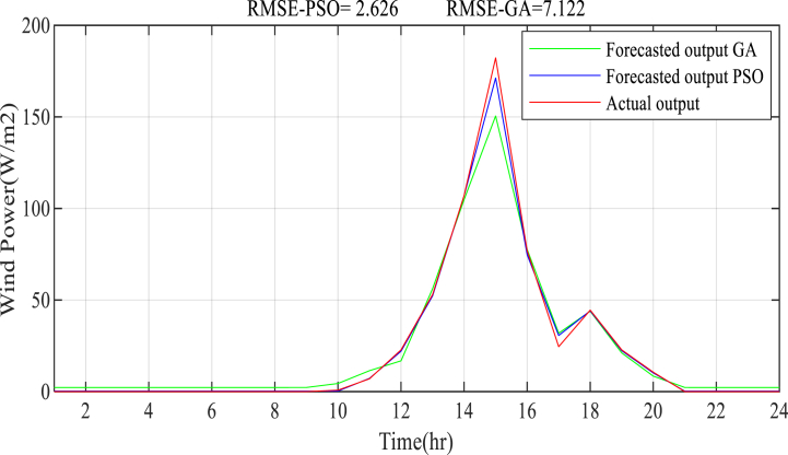
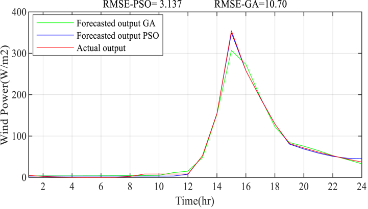
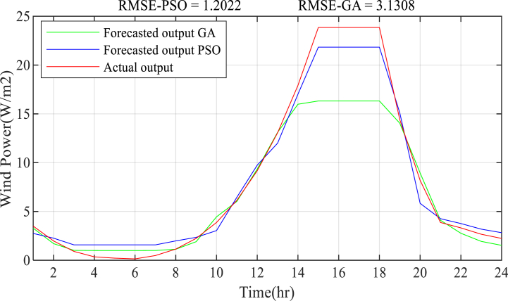
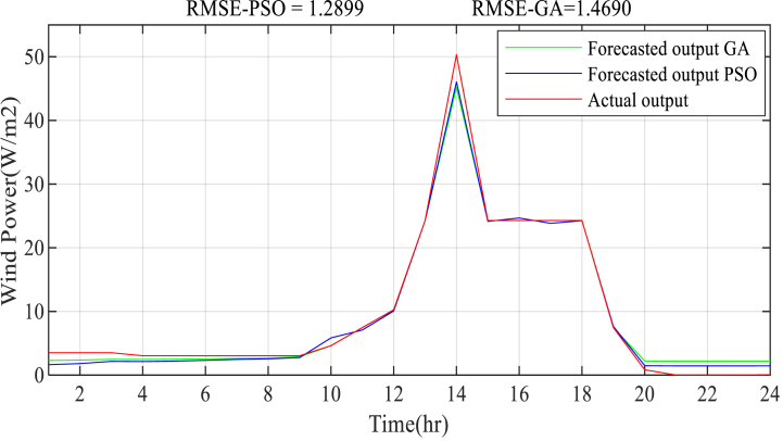
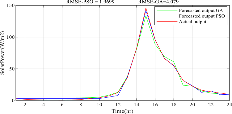
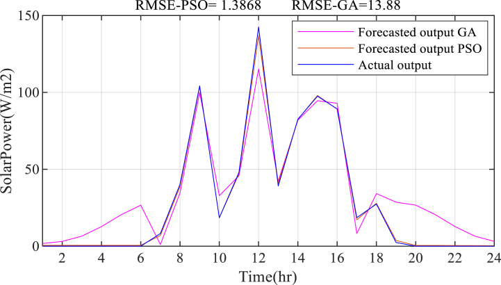
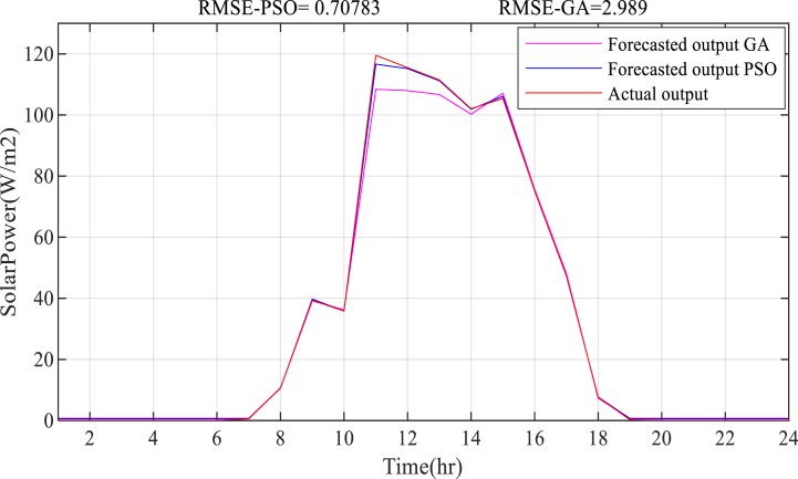
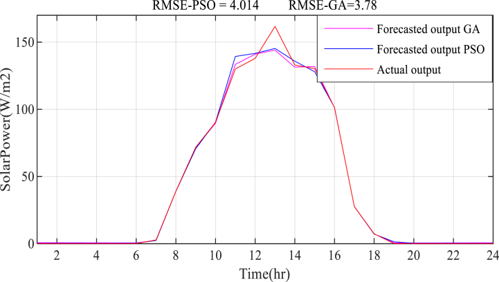
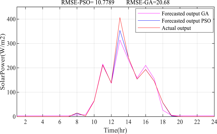
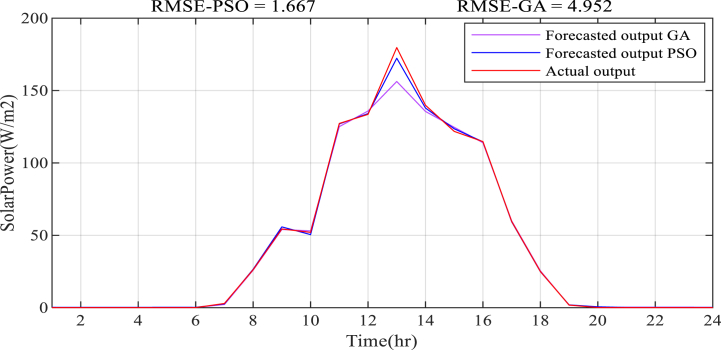
The results of both the wind and solar power forecasting models using Fuzzy-PSO and Fuzzy-GA (with no ECF input) prediction approaches on a seasonal basis are presented in Figs. Fig. 11, Fig. 12, Fig. 13, Fig. 14, Fig. 15, Fig. 16, Fig. 17, Fig. 18, Fig. 19, Fig. 20. The cost function introduced in Eqs. (22)–(24) has been applied to the proposed Fuzzy-PSO and Fuzzy-GA wind and solar power forecasting models to measure the accuracy level of the forecast. The results in Tables 5 and 6 summarizes the performance of the proposed hybrid Fuzzy-PSO, fuzzy-alone, and Fuzzy-GA wind and solar power forecasts. The performance metrics of the three-cost functions in Eqs. (22)–(24)) clearly indicate the newly introduced Fuzzy-PSO model has an outstanding performance over the other modeling approaches which are presented in both Tables 5 and 6 The best fitness values in terms of MAPE of wind and solar power prediction results using the proposed Fuzzy-PSO model are 1.36% (Winter season) and 2.42% (Winter season) whereas the result using Fuzzy-GA 6.34% (Winter season) and 4.35% (Spring season) and Fuzzy-alone models are 5.67% (Spring season) and 16.26% (Fall season) respectively. Due to the addition of a new input parameter (ECF) to the proposed Fuzzy-PSO model, a high degree of accuracy is shown.

Fig. 11.

Fuzzy-PSO prediction of wind power in Fall.

Fig. 12.

PSO-Fuzzy prediction of wind power in Winter.

Fig. 13.

Fuzzy-PSO prediction of wind power in Spring.

Fig. 14.

PSO-Fuzzy prediction of wind power in Summer.

Fig. 15.

Yearly average wind power prediction result.

Fig. 16.

Solar power prediction result in Fall season.

Fig. 17.

Solar power prediction result in Winter season.

Fig. 18.

Solar power prediction result in Spring season.

Fig. 19.

Solar power prediction result in Summer season.

Fig. 20.

Average Solar power prediction result to model a microgrid.

Table 5.

Performance evaluation of the wind power prediction model and the optimized generated rules.

Seasonal	Algorithms
	Fuzzy-alone			Fuzzy-GA			Fuzzy-PSO			Initial rules	Optimized PSO rules
	RMSE	NRMSE	MAPE	RMSE	NRMSE	MAPE	RMSE	NRMSE	MAPE
Fall Season	29.25	1.2339	27.37	7.12	0.1321	12.47	2.63	0.0507	2.37	27	17
Winter Season	68.77	0.1941	23.45	10.70	0.0302	6.34	3.14	0.0089	1.36	27	17
Spring Season	3.38	0.0185	5.67	3.13	0.0391	7.21	1.02	0.0144	4.95	27	14
Summer Season	5.27	0.1047	16.75	1.47	0.2920	21.23	1.29	0.0256	5.92	27	19
System Average	15.08	0.1037	15.24	4.08	0.0281	8.46	1.97	0.0136	4..23	27	21

Table 6.

Performance evaluation of the solar PV power prediction model and the PSO optimized generated rules.

Seasonal	Algorithm
	Fuzzy-alone			Fuzzy-GA			Fuzzy-PSO			Initial rules	Optimized PSO rules
	RMSE	NRMSE	MAPE	RMSE	NRMSE	MAPE	RMSE	NRMSE	MAPE
Fall Season	15.25	0.0943	16.26	13.89	0.0859	14.23	1.387	0.0086	3.36	135	98
Winter Season	17.44	0.1460	23.43	2.99	0.0250	8.43	0.708	0.0059	2.42	135	29
Spring Season	19.24	0.1350	24.15	3.78	0.0265	4.35	4.014	0.0282	5.47	135	41
Summer Season	68.98	0.1697	32.68	20.68	0.0509	10.27	10.78	0.0265	6.21	135	98
System Average	12.14	0.0676	12.79	4.95	0.0276	6.34	1.67	0.0093	3.74	135	87

Tables 7 and 8 demonstrate the correlation between the input and output of the fuzzy-GA and fuzzy-PSO prediction models in terms of the correlation parameters, R and R². R and R² are the measure of the degree of correlation between the predictor (input) and response (output) variables. Stronger correlation between the predictor and response variable is indicated by higher values of R and R². In Table 7, the historical wind power input variables have a strong correlation (R20.94) with the forecasted wind power as compared to the remaining input variables. In Table 8, the temperature, ECF, and historical solar PV power have a significant correlation with the predicted solar PV power. In general, compared to the Fuzzy-GA prediction model, the Fuzzy-PSO model offers a stronger correlation between the input and anticipated output variables of both solar PV and wind power.

Table 7.

Correlation coefficients of input and output variables of wind power prediction model.

Seasonal	Correlation Coefficients/Forecasted Power/
	Fuzzy-GA				Fuzzy-PSO
	time		Hpower		time		Hpower		ECF
	R	R2	R	R2	R	R2	R	R2	R	R2
Fall Season	0.211	0.044	0.946	0.895	0.211	0.045	0.949	0.898	0.410	0.168
Winter Season	0.430	0.185	0.978	0.957	0.439	0.193	0.982	0.963	0.338	0.114
Spring Season	0.405	0.164	0.973	0.947	0.414	0.171	0.977	0.955	0.216	0.047
Summer Season	0.215	0.046	0.959	0.920	0.225	0.051	0.956	0.915	0.618	0.382
System Average	0.343	0.118	0.974	0.949	0.413	0.171	0.977	0.954	0.109	0.012

Table 8.

Correlation coefficients of input and output variables of solar PV power prediction model.

Seasonal	Correlation Coefficients/Forecasted Power/
	Fuzzy-GA						Fuzzy-PSO
	time		Temperature		Hpower		time		Temperature		Hpower		ECF
	R	R2	R	R2	R	R2	R	R2	R	R2	R	R2	R	R2
Fall Season	0.03	0.001	0.645	0.416	0.940	0.884	0.08	0.006	0.643	0.413	0.903	0.816	0.914	0.836
Winter Season	0.065	0.004	0.727	0.528	0.974	0.948	0.07	0.004	0.736	0.541	0.973	0.947	0.974	0.948
Spring Season	0.02	0.000	0.83	0.686	0.994	0.989	0.019	0.000	0.830	0.689	0.994	0.988	0.908	0.824
Summer Season	0.121	0.015	0.796	0.654	0.980	0.961	0.12	0.014	0.803	0.645	0.970	0.941	0.598	0.356
System Average	0.075	0.006	0.808	0.653	0.987	0.975	0.078	0.006	0.816	0.665	0.989	0.978	−0.30	0.09

4.1. Prediction of wind power using Fuzzy-PSO algorithm

The wind power prediction results on a seasonal basis are presented in Figs. Fig. 11, Fig. 12, Fig. 13, Fig. 14, Fig. 15. The result is based on the estimation of wind power from the wind speed data using an empirical formula. For each season, the energy from wind, is calculated from the available wind speed at a height of 50 m. The hourly calculated wind power-based yearly averages in 2017 and 2018 is considered as the training input dataset along with the ECF and the time of day, whereas the hourly wind power is based on the yearly average in 2019 that is used to validate the model. The simulation result shows, the Fuzzy-PSO wind prediction model effectively forecasts the wind power generation in the next 24 h with a maximum RMSE of 3.14 during the winter season and maximum prediction RMSE accuracy of 1.02 during the Spring season. The Fuzzy-PSO wind power forecasting model is capable of accurately estimating the short-term power output of wind turbines.

The proposed Fuzzy-PSO model outperforms the Fuzzy-alone, Fuzzy-GA, and previously established prediction models provided in Table 1. Based on the RMSE, the NRMSE, and the MAPE performance measurement index presented in Table 5, the Fuzzy-PSO wind power generation forecast model has superior performance. As we have seen from the wind power prediction result shown in Figs. 11–15 the proposed Fuzzy-PSO prediction model has superior performance, especially at higher wind power generation values, than the Fuzzy-alone and Fuzzy-GA forecasting models.

In terms of the RMSE, NRMSE, and MAPE criterion, the Fuzzy-PSO model has performed significantly better than the fuzzy-alone and Fuzzy-GA models. The Fuzzy-PSO wind power prediction model easily beat both fuzzy-alone and Fuzzy-GA models throughout the forecasting seasons, which is presented in Table 5 as a comparison result. All of the findings verify the proposed method's capacity to directly estimate wind power from daily meteorological data with fair accuracy and superior precision to existing forecasting methodologies.

4.2. Prediction of Solar Power using Fuzzy-PSO Algorithm

The solar power prediction result on a seasonal basis is presented in Figs. Fig. 16, Fig. 17, Fig. 18, Fig. 19, Fig. 20. The estimation of solar power using an empirical formula is used to forecast solar power generation. The available solar irradiation and temperature data are used to determine the solar PV power for each season. The average calculated power for each season in 2017 and 2018 is considered as the training input dataset along with the temperature data, ECF, and time of the day, whereas the Fuzzy-PSO forecasting model is validated using the average solar PV power in 2019. The proposed Fuzzy-PSO solar power prediction model effectively forecasts the solar power in the next 24 h with a maximum RMSE of 10.78 and a MAPE of 6.21% during summer season. The best RMSE value of 0.708 and MAPE of 2.42% during the winter season is obtained. In general, the Fuzzy-PSO solar power prediction model can effectively forecast the short-term power generation of solar PV systems with a high level of accuracy.

The Fuzzy-PSO solar power prediction model performed significantly better than the fuzzy-alone and Fuzzy-GA forecasting models according to the cost function standard measure in Table 6, the RMSE, NRMSE, and MAPE criterion, only falling behind during the spring season. The Fuzzy-PSO solar PV power prediction model has outperformed both fuzzy-alone and fuzzy-GA models throughout the four seasons, including the overall system average solar power forecast result shown in Fig. 20. The overall solar power prediction result verify the new technique's ability to precisely forecast solar power from daily weather variables with superior precision than the other forecasting methodologies stated in this paper and in the introduction section of Table 1.

Using a two-year training and one-year validation dataset of the Fuzzy-PSO forecasting model of both solar PV and wind power is one of the limitations of this research. Considering a longer period of training and validation dataset (>5 years) in the Fuzzy-PSO wind and solar power forecasting model is expected to enhance the effectiveness and accuracy of the model.

5. Conclusion

The Fuzzy-PSO-based hybrid strategy is developed in this paper for short-term wind and solar power forecasts by introducing a new fuzzy input variable called the ECF. To verify its performance with fuzzy-alone and fuzzy-GA forecasting techniques, a comparison study was conducted. The simulation results for both wind and solar power forecasting models demonstrate the proposed Fuzzy-PSO forecasting model provides a substantial improvement over the conventional Fuzzy-alone and Fuzzy-GA forecasting models. In addition to that, the Fuzzy-PSO forecasting model is an effective and autonomous technique to manipulate a substantial amount of data from the past that is used for prediction modeling where the perfect correlation between the input and output variables is difficult to determine using statistical techniques. The RMSE, the NRMSE, and the MAPE are considered as an indicator of the performance of the proposed approaches. The RMSE of the proposed approach for the average wind and solar power prediction models are 1.97 and 1.67 respectively which is far better than the fuzzy-alone and Fuzzy-GA prediction models of an RMSE value of 4.08 for wind and 4.95 for solar PV. The effectiveness of the proposed technique in terms of MAPE for the average wind power prediction model is 4.23% and for the solar PV power prediction model is 3.74%, which is far superior than the fuzzy-alone and Fuzzy-GA forecasting models whose MAPE of 8.46% and 6.34% for wind and solar PV power prediction models respectively.

Conflicts of Interest: The authors declare no conflict of interest regarding the publication of this research article.

Declarations

CRediT Author Statement

Demsew Mitiku Teferra: Methodology, Software, Validation, Formal analysis, Investigation, Data Curation.

Livingstone M.H.Ngoo: Data Curation, Resources, Writing - Original Draft, Supervision.

George N. Nyakoe: Data Curation, Resources, Writing - Review & Editing, Supervision, Visualization.

Funding statement

This research did not receive any specific grant from funding agencies in the public, commercial, or not-for-profit sectors.

Data availability statement

Data will be made available on request.

Declaration of interest's statement

The authors declare no competing interests.

References

- 1.Yadav Harendra K., Pal Y., Tripathi Madan Mohan. Annual IEEE India Conference; December 2015. Photovoltaic Power Forecasting Methods in Smart Power Grid; pp. 1–6. [Google Scholar]
- 2.Sun Q., Huang B., Li D., Ma D., Zhang Y. Optimal placement of energy storage devices in microgrids via structure preserving energy function. IEEE Trans. Ind. Inf. June 2016;12(3):1166–1179. [Google Scholar]
- 3.Li C.D., Wang L., Zhang G.Q., Wang H.D., Shang F. Functional-type single-input-rule-modules connected neural fuzzy system for wind speed prediction. IEEE/CAA Journal of Automatica Sinica. 2017;4(Issue. 4):751–762. [Google Scholar]
- 4.Catalao J.P., Pousinho H.I., Mendes V.F. Hybrid wavelet PSO-ANFIS approach for short term electricity prices forecasting. IEEE Trans. Power Sys. February 2010;26(Issue.1) page 137–144. [Google Scholar]
- 5.Khatib T., Mohamed A., Mahmoud M., Sopian K. Modeling of daily solar energy on a horizontal surface for five main sites in Malaysia. Int. J. Green Energy. 2011;8(8):795–819. doi: 10.1080/15435075.2011.602156. [DOI] [Google Scholar]
- 6.Zeng J., Qiao W. Power and Energy Society General Meeting. IEEE. IEEE; 2011. Short-term solar power prediction using an RBF neural network; pp. 1–8. 2011. [Google Scholar]
- 7.Voyant C., Muselli M., Paoli C., Nivet M.L. Numerical weather prediction (NWP) and hybrid ARMA/ANN model to predict global radiation. Energy. 2012;39(1):341–355. doi: 10.1016/j.energy.2012.01.006. [DOI] [Google Scholar]
- 8.Jafarzadeh S., Fadali M.S., Etezadi-Amoli M. Power and Energy Society General Meeting. IEEE. IEEE; 2012. Fuzzy type-1 and type-2 TSK modeling with application to solar power prediction; pp. 1–6. 2012. [Google Scholar]
- 9.Shi J., Guo J., Zheng S. Evaluation of hybrid forecasting approaches for wind speed and power generation time series. Renew. Susta. Energy Rev. 2012;16(Issue- 5) page 3471–3480. [Google Scholar]
- 10.Yang H.T., Huang C.M., Huang Y.C. A weather-based hybrid method for 1-day ahead hourly forecasting of PV power output,” IEEE Transa. on Sustana. Energy. 2014;5(3):917–926. [Google Scholar]
- 11.Yadav Harendra K., Pal Y., Tripathi Madan Mohan. A novel GA ANFIS hybrid model for short term solar PV power forecasting in Indian electricity market. J. Inf. Optim. Sci. 2019;40(Issue-2):377–395. [Google Scholar]
- 12.Almaraashi M. Short-term prediction of solar energy in Saudi Arabia using automated-design fuzzy logic systems. PLoS One. 2017;12(8) doi: 10.1371/journal.pone.0182429. [DOI] [PMC free article] [PubMed] [Google Scholar]
- 13.Zhong Y.-J., Wu Y.-K. 2020. Short-Term Solar Power Forecasts Considering Various Weather Variables," 2020 International Symposium on Computer, Consumer and Control (IS3C) pp. 432–435. [DOI] [Google Scholar]
- 14.Serttas F., Hocaoglu F.O., Akarslan E. 2018. Short Term Solar Power Generation Forecasting: A Novel Approach," 2018 International Conference on Photovoltaic Science and Technologies (PVCon) pp. 1–4. [DOI] [Google Scholar]
- 15.Yang X., Jiang F., Liu H. 2nd IET Renewable Power Generation Conference; 2019. Short-term Solar Radiation Prediction Based on SVM with Similar Data; pp. 1–4. RPG 2019. [DOI] [Google Scholar]
- 16.Rendroyoko I., Suhana H.H., Besanger Y. 2021. Hourly Day-Ahead Solar Energy Prediction for Supporting Smart Grid Implementation in Semau Island," 2021 3rd International Conference on High Voltage Engineering and Power Systems (ICHVEPS) pp. 108–111. [DOI] [Google Scholar]
- 17.Wang L., Wang Z., Wang B. POWERCON); 2018. Wind Power Day-Ahead Prediction Based on LSSVM with Fruit Fly Optimization Algorithm," 2018 International Conference on Power System Technology; pp. 999–1003. [DOI] [Google Scholar]
- 18.Chen G., et al. 2019. Research on Wind Power Prediction Method Based on Convolutional Neural Network and Genetic Algorithm," 2019 IEEE Innovative Smart Grid Technologies - Asia (ISGT Asia) pp. 3573–3578. [DOI] [Google Scholar]
- 19.Rafique Syed Furqan, Zhang Jianhua, Rafique Rizwan, Guo Jing, Jamil Irfan. Renewable generation (Wind/Solar) and Load modeling through modified fuzzy prediction interval. Int. J. Photoenergy. 2018:14. doi: 10.1155/2018/4178286. Article ID 4178286. [DOI] [Google Scholar]
- 20.Kassa Semero Yordanos, Zheng Dehua, Zhang Jianhua. A PSO-ANFIS based hybrid approach for short term PV power prediction in microgrids. Elec. Power Compon. Syst. 2018 doi: 10.1080/15325008.2018.1433733. [DOI] [Google Scholar]
- 21.Zheng Dehua, Kassa Semero Yordanos, Zhang Jianhua, Wei Dan. Wiley Online Library (wileyonlinelibrary.com; 2018. Short-Term Wind Power Prediction in Microgrids Using a Hybrid Approach Integrating Genetic Algorithm, Particle Swarm Optimization, and Adaptive Neuro-Fuzzy Inference Systems”, IEEJ TRANSACTIONS on ELECTRICAL and ELECTRONIC ENGINEERING IEEJ Trans. Published online in. [DOI] [Google Scholar]
- 22.Seyed A.M.M., Hizam H., Chandima G. Estimation of hourly, daily and Monthly global solar radiation on Inclined surfaces: models Re-Visited. Energies. 2017;10:134. doi: 10.3390/en10010134. [DOI] [Google Scholar]
- 23.Solar cell parameters and Equivalent circuits: solar energy facts. https://ocw.tudelft.nl/wpcontent/uploads/solar_energy_section_9_1_9_3.pdf
- 24.Mengi O.O., Hakkı Altas I. Fuzzy logic control for a wind/battery renewable energy production system. Turk. J. Electr. Eng. Comput. Sci. 2012;20(2):187–206. [Google Scholar]
- 25.Gijis A.M., Kuik V. The Lanchester-Betz Joukowsky limit. Wind Energy. 2007;10(3):289–291. doi: 10.1002/we.218. [DOI] [Google Scholar]
- 26.Kennedy J., Eberhart R. Particle Swarm Optimization. 1995. pp. 1942–1948. [DOI] [Google Scholar]
- 27.Shi Y.H., Eberhart R. Proceedings of the International Conference on Evolutionary Computation. 1999. A modified particle swarm optimizer; pp. 1945–1950. Washington. [Google Scholar]
- 28.Teferra D.M., Ngoo L.M.H., Nyakoe G.N. 2021. A Fuzzy Based Prediction of an Industrial Load in Microgrid System Using Particle Swarm Optimization Algorithm," 2021 International Conference on Electrical, Computer, Communications and Mechatronics Engineering (ICECCME) pp. 1–6. [DOI] [Google Scholar]
- 29.Teferra Demsew Mitiku, Ngoo Livingstone M.H., Nyakoe George N. Fuzzy-swarm intelligence-based short-term Load forecasting model as a solution to power quality issues existing in microgrid system. Journal of Electrical and Computer Engineering. 2022;2022 doi: 10.1155/2022/3107495. Article ID 3107495, 14 pages. [DOI] [Google Scholar]
Associated Data
This section collects any data citations, data availability statements, or supplementary materials included in this article.