Summary
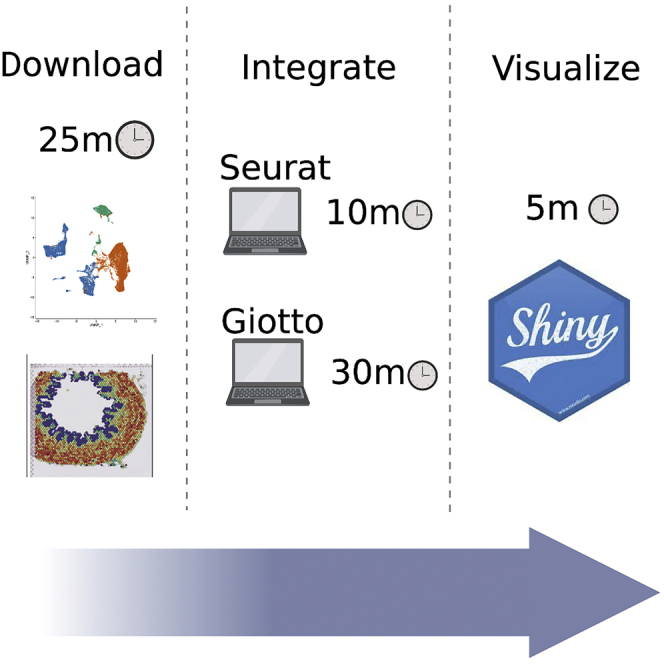
There is a wealth of software that utilizes single-cell RNA-seq (scRNA-seq) data to deconvolve spatial transcriptomic spots, which currently are not yet at single-cell resolution. Here we provide protocols for implementing Seurat and Giotto packages to elucidate cell-type distribution in our example human ureter scRNA-seq dataset. We also describe how to create a stand-alone interactive web application using Seurat libraries to visualize and share our results.
For complete details on the use and execution of this protocol, please refer to Fink et al. (2022).1
Subject areas: Bioinformatics, Single Cell, Sequencing, RNAseq
Graphical abstract
Highlights
-
•
Two approaches for integrating scRNA-seq profiles with spatial expression data
-
•
Guide for comparing these protocols to determine which is best for a given dataset
-
•
Scripts for download of sample data and setup for both protocols
-
•
The code to run an interactive RShiny app for integrated spatial data
Publisher’s note: Undertaking any experimental protocol requires adherence to local institutional guidelines for laboratory safety and ethics.
There is a wealth of software that utilizes single-cell RNA-seq (scRNA-seq) data to deconvolve spatial transcriptomic spots, which currently are not yet at single-cell resolution. Here we provide protocols for implementing Seurat and Giotto packages to elucidate cell-type distribution in our example human ureter scRNA-seq dataset. We also describe how to create a stand-alone interactive web application using Seurat libraries to visualize and share our results.
Before you begin
This protocol demonstrates how to perform integration of Visium spatial gene expression data with single-cell RNA-seq data using two tools: Seurat2 and Giotto3. We chose these tools because they were the most commonly used integration tools during our methods survey in September, 2021. Prior to this analysis, we had performed scRNA-seq and immunofluorescence staining on the same samples. We used results from these orthogonal approaches as a ground truth, and our aim was to select the integration method that rendered the most consistent results.
In order to perform the following analysis, you must first obtain the appropriate software and scripts. Additionally, we have provided test data to perform this protocol from Fink et al.1 As long as the appropriate files are prepared, this protocol should work with any pair of matching scRNA-seq and Visium dataset.
Download scripts from GitHub
Timing: 5–10 min(for step 1)
Timing: 15 min (for step 2)
-
1.Download necessary scripts.
-
a.If you are on a Mac or Linux platform then the following snippet can be used to “clone” the repository into your working directory.
-
b.If you are on a Windows platform, download the code in the form of a .zip file from the repository’s web page. After downloading the zip file, decompress the file and ensure all the contents are identical to the GitHub repository.
-
c.The above steps downloads the entire sge-integration github repository to your current directory, with scripts folder (containing all scripts described here), shiny-app folder (containing shiny app related scripts) and figures folder (with Giotto and Seurat as blank subfolders) to save your output from the respective workflows.Note: A repository of code has been prepared to aid in this protocol at https://github.com/tingalab/sge-integration. This code includes all the snippets shown in this protocol, as well as code that can be used to download the test data. Additionally, comments have been made on this code to complement the instructions in this protocol.
-
a.
-
2.
Use our script install_dependencies.R to install these packages. Specific instructions are provided within the script as comments.
Note: All the required tools and dependencies are listed below in the key resources table.
CRITICAL: It is imperative that the users install the specified version (or higher) for each dependency listed in the materials and equipment section.
-
3.
In order to facilitate setup, a script (setup.R) is provided in the repository downloaded in Setup step 1. Running this script in R downloads all the necessary data.
Note: The dataset in this protocol consists of a scRNA-seq dataset and two samples of 10× Visium spatial gene expression. Both the scRNA-seq and Visium expression data have been processed according to Fink et al.1 The data is provided in two ways – one through a release on GitHub and another via GEO submission.
Key resources table
Step-by-step method details
Perform integration in Seurat
Timing: 5–10 min (for step 1)
We use Seurat to elucidate scRNA-seq derived identities in the spatial data. We found this method to be the most effective. While Seurat does not successfully map all cell types, it still offers the highest accuracy when compared to our expectations. This major step informs the use of Seurat for integration so that you can make your own decision about your data. Users can run this workflow using Seurat.R script.
-
1.Load scRNA-seq dataset and Seurat packages.
-
a.Navigate to the directory you downloaded from GitHub in the setup (this directory should be named “sge-integration”).
-
b.Run the following code in R.
-
a.
library(Seurat)
library(dplyr)
library(tidyverse)
library(purrr)
library(janitor)
library(magrittr)
library(patchwork)
library(stringr)
library(R.utils)
#--------Setup-------
homedir<-"/home/sonas/star_protocol"
setwd(paste0(homedir,"/sge-integration/"))
source("scripts/functions.R")
scRNA <- readRDS(file = "data/scRNA/ureter-scRNA.Rds")
genes<-read.csv(file ="data/scRNA/genes.csv")[,1]
source("scripts/functions.R")
-
2.Load the Visium samples.
-
a.Use the function defined in the “functions.R” script called preProcessVisiumSeurat().
-
b.This function loads the provided data into a usable “Seurat” object, calculates mitochondrial gene % per spot, log-normalizes the data, finds variable features, and then performs principal component analysis (PCA) on the re-scaled data.
-
a.
Note: The function preProcessSeuratVisium() in functions.R script consolidates all these steps and can be executed as follows:
U2.Seurat <- preProcessSeuratVisium("data/U2", normalization = "LogNormalize")
-
3.
Integrate the loaded, pre-processed Visium data with the scRNA-seq data. Seurat utilizes an anchor-gene approach, which we have compacted into one function as anchorMapping().
U2.Seurat <- anchorMapping(scRNA, U2.Seurat, feats = genes, query.dims=30, anchor.labels = levels(as.factor(scRNA$subclass)))
Note: Try changing the number of dimensions in the “query.dims” parameter to tweak your results. This parameter adjusts the number of PCA dimensions used for the Visium data. Be careful, however, not to overestimate this as an excess of query dimensions can lead to overfitting of single-cell signatures on the Visium data.
-
4.
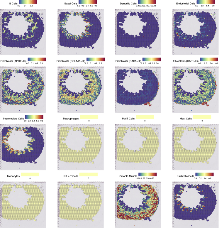
Plot the predicted signatures on the Visium sample on top of the H&E image of the tissue. The following lines of code are used to plot all single-cell identities altogether in one output (Figure 1).
scplots <- purrr::map(levels(as.factor(scRNA$subclass)), function(x) SpatialFeaturePlot(U2.Seurat, x) +
theme(legend.key.size = unit(10, "mm"),
legend.text = element_text(size = 15),
legend.title = element_text(size = 20)))
patchwork::wrap_plots(scplots, ncol=4) %T>% ggsave(filename = "figures/Seurat/Figure_1.pdf", width = 25, height = 25, units = "in", dpi = 300)
Note: To plot them separately, see the commented code in the “Seurat.R” file.
Figure 1.
Integration results with Seurat
Single-cell identities are plotted onto Seurat-processed Visium data. Integration scores represent relative correspondence. Plots that are entirely yellow indicate identities not found.
Perform integration with Giotto
Timing: 15 – 30 min. depending on image alignment (for step 5)
This portion of the protocol describes the use of Giotto to predict cell type in Visium data. Giotto seemed to be more effective than other methods at detecting sparse cell types, such as immune cells. However, we found that the signal for anatomically well-established cell types, such as stromal and urothelial cell types, was overly diffuse when compared to other methods. Nonetheless, this section allows you to determine if Giotto might be appropriate for your dataset. Users can run this workflow using Giotto.R script.
-
5.Giotto Setup: Giotto has its own file format, and so we must do a little extra setup before performing the analysis. Follow steps below to setup for Giotto.
-
a.Set up the environment, functions, and packages needed to run Giotto.library(Giotto)library(ggplot2)library(viridis)mydir='/home/sonas/star_protocol/'setwd(paste0(mydir,"sge-integration/"))source("scripts/functions.R")scRNA <- readRDS("data/scRNA/ureter-scRNA.Rds")#----- Configure workspace with Giottoresults_folder = 'figures/Giotto'instrs = createGiottoInstructions(save_dir = results_folder,save_plot = TRUE,show_plot = FALSE)
 CRITICAL: You need to change the working directory in the “setwd()” line to your local path. The other paths should be fine as long as you set the working directory to the “sge-integration” folder.
 -
b.Create a Giotto object using the provided sample data. If you use your own Visium data, you need to change the adjustment factors (see troubleshooting 1).
-
a.
U2 <- createGiottoVisiumObject(visium_dir = 'data/U2', expr_data = 'filter',
h5_visium_path = 'data/U2/filtered_feature_bc_matrix.h5',
h5_tissue_positions_path = 'data/U2/spatial/tissue_positions_list.csv',
h5_image_png_path = 'data/U2/spatial/tissue_lowres_image.png',
gene_column_index = 2, instructions = instrs, xmax_adj = 2000, ymin_adj = 1500, ymax_adj = 1600, xmin_adj = 1400)
-
6.Pre-process the Visium data in the “Giotto” object format (identical to the suggested steps in the Giotto vignette).
-
a.Log-normalize (same scaling factor as with Seurat).
-
b.Calculate highly variable genes.
- c.
-
d.PCA is then invoked on those genes.
-
e.Giotto creates a spatial network, which allows further functions to perform as intended.
-
f.Plot the PCA results and the spatial network formed by the Visium spots.
-
a.
Note: We perform this pre-processing on our example data as follows:
U2.Giotto<- preProcessGiotto(U2, "U2")
-
7.After the Visium data is processed and ready for integration, we then move on to performing the integration itself. Giotto requires you to first create a signature matrix and then to integrate using the “rank” method.
-
a.Create a signature matrix using the scRNA-seq data by running the following:sc_sign_matrix <- makeSignMatrixRank(sc_matrix = as.matrix(scRNA@assays$RNA@data),sc_cluster_ids = scRNA$subclass,ties_method = c("random"),gobject = NULL)
-
b.Run the actual function to perform spatial enrichment of signatures from the signature matrix.
-
a.
U2.Giotto <- runSpatialEnrich(
U2.Giotto,
enrich_method = c("rank"),
sign_matrix = sc_sign_matrix,
expression_values = c("normalized"),
)
-
8.
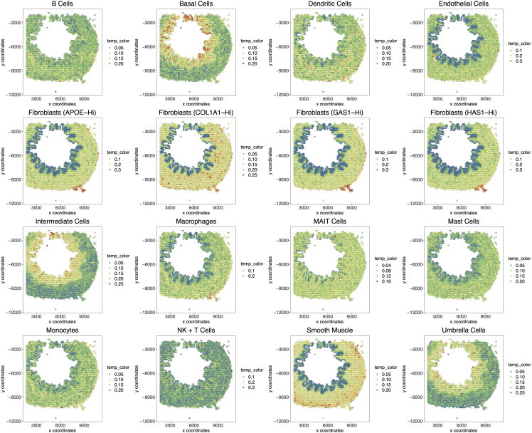
Obtain a visualization of the results of spatial enrichment of signatures (Figure 2) by running the following code:
scplots <- purrr::map(levels(as.factor(scRNA$subclass)), function(i) spatPlot(gobject = U2.Giotto, cell_color=unlist(c(U2.Giotto@spatial_enrichment$rank[,..i])), point_size = 2) +
theme(title = element_text(size=18),
legend.text = element_text(size = 15),
legend.title = element_text(size = 15),
axis.title = element_text(size=15),
axis.text = element_text(size=15)) +
ggtitle(i) + scale_fill_distiller(palette = “Spectral”))
patchwork::wrap_plots(scplots, ncol=4) %T>% ggsave(filename = "figures/Giotto/Figure_2.pdf", width = 25, height = 20, units = "in", dpi = 300)
Figure 2.
Giotto spatial enrichment
Single-cell signatures are plotted onto Giotto-processed Visium data. Scores are calculated using a rank-biased method (for more details see https://rubd.github.io/Giotto_site/reference/runRankEnrich.html).
Create a RShiny app with Seurat-integrated data
Timing: 5–10 min (for step 9)
Once we determined that Seurat integration results are most consistent with our experimental observations, we created an interactive application to democratize access to the results. This final section in the protocol allows you to make an interactive RShiny app with your integrated data. For this, we repurposed code from Seurat to produce an interactive viewing platform that can be hosted on the web and shared.
-
9.
Edit data object in Shiny app script and run all the code provided in that script to prepare the data and shiny app. In order to specify our own data, edit lines 12–13, shown below. You need to assign the variable “object” a Seurat spatial dataset.
object <- U2.Seurat
Note: The script responsible for the app (app.R) can be found under the `shiny-app` directory in the codebase retrieved from GitHub.
Note: If you are in an interactive R session and your object is in your current workspace, you can assign the variable as above. In other scenarios, such as when setting up a Shiny app on a hosted web server, you may want to load the data from a file.
CRITICAL: The app only supports Seurat objects as input. Therefore, Giotto is not a supported format to share via this Shiny app.
-
10.
Launch the Shiny app by runing the following line:
>runApp(‘shiny-app’)
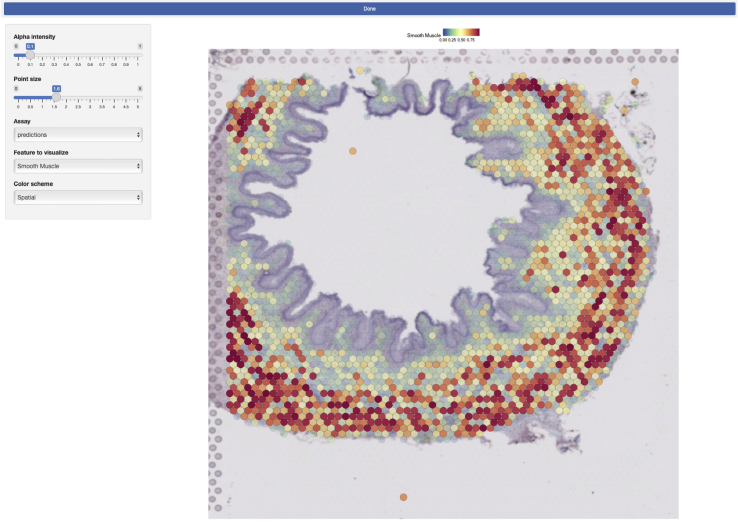
Note: See the output of this command to find where the app has launched. When using an environment such as RStudio, the app launches in a pop-up browser window (Figure 3).
Figure 3.
Shiny app visualization
Seurat-integrated single-cell identities have been made available through an interactive R Shiny app.
Expected outcomes
The major expected outcome of this protocol is two sets of results which elucidate the spatial enrichment for single-cell signatures, allowing the user to select the method that works best for their dataset. These outcomes are generated by running the lines of code in the protocol. The code saves each figure as a persistent PDF file. Additionally, two R data objects are generated corresponding to the two methods to be saved and/or analyzed further at your discretion.
Another major outcome of this protocol is the ability to visualize the data in an interactive web app. This is valuable because it democratizes the ability to generate figures using the data. The app allows those who lack the coding expertise to derive figures themselves by simply selecting features from a drop-down menu. It also affords the data a greater scientific reach by allowing journal readers the opportunity to explore and possibly utilize the evidence you have gathered.
Limitations
One major limitation of this protocol is that it only covers two methods for this operation. There may exist additional methods in the literature, however an exhaustive benchmarking of all available integration tools is outside the scope of this protocol. We also acknowledge that the performance of these tools may be dataset dependent, which we have not systematically evaluated since we only worked with our own dataset on the human ureters.
The Shiny app presented in this protocol is only usable with Seurat-formatted data, therefore plotting Giotto results is not supported. Additionally, the Shiny app is limited by the number of features it can plot. When the web app has to visualize more than 5,000 genes, it becomes slow or crashes sporadically. For this reason, we have limited the number of genes plotted by the Visium app.
Troubleshooting
Problem 1
When using your own dataset for integration using Giotto, the spots in Giotto do not align to the background image.
Potential solution
Adjust the parameters xmax_adj, xmin_adj, ymin_adj, ymax_adj. These control how your background image is scaled to fit on the grid of spots used to visualize Visium data. Every dataset may differ slightly. A line of code containing the spatPlot function is commented out in the Giotto.R script to aid in a trial-and-error approach for aligning the image to the spot grid.
Problem 2
When integrating using Seurat, identities do not show up where they are expected to or do not match previously elucidated biological insight.
Potential solution
Slight adjustments to various algorithm parameters may lead to better results. Our suggestion is to gain familiarity with what each parameter represents and tweak the parameter according to biological context. For example, Visium samples with more homogenous cell types may require less PCs used when integrating with Seurat while more diverse samples may require more.
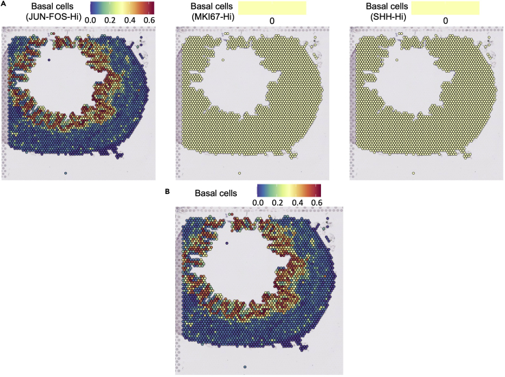
One tactic we employed in preparing results for Fink et al.1 is grouping similar cell subtypes to produce more accurate results. For example, we had multiple subtypes of basal cells with distinct gene expression patterns from the scRNA-seq experiment. This specificity, however, did not carry over to Visium (Figure 4A), most likely due to the limited resolution of the current Visium platform. As a result, we grouped the basal cell subtypes together so that we may see where all basal cells lie, rather than where a specific subtype resides (Figure 4B).
Figure 4.
Grouping identities together can produce more interpretable results
(A) Individual basal cell subtypes derived from scRNA-seq could not be mapped successfully.
(B) When we combined all the basal subtypes into one basal cell type, the merged group mapped nicely to the expected location within the tissue.
Problem 3
You may see the following error message appear when using plotting functions for integration using Giotto:
> Warning: `guides(<scale> = FALSE)` is deprecated. Please use `guides(<scale> = "none")` instead.
Potential solution
As of now, we have not noticed any downsides to this error message so it can be ignored.
Problem 4
Dependent on the operating system used to perform this protocol, there may be a range of difficulties installing Giotto for integration using Giotto.
Potential solution
According to the Giotto GitHub Pages site, the preferred method of installation is using the following code.
library(devtools) # if not installed: install.packages('devtools')
library(remotes) # if not installed: install.packages('remotes')
remotes::install_github("RubD/Giotto@v1.1.0")
In addition, the authors of Giotto offer extensive troubleshooting for common issues here https://giottosuite.readthedocs.io/en/master/. It should be noted that this protocol installs all necessary Python packages via conda (as demonstrated in Giotto.R) and should NOT be manually installed.
Problem 5
If there is incompatibility in the normalization methods, Seurat-based integration workflow may generate error and prevent the integration of scRNA-seq data to spatial data.
Potential solution
It should be noted that in order for Seurat-formatted objects to be integrated with one another (such as in the Seurat.R script), they must be normalized in the same manner. For instance, we have performed the log normalization workflow for both our single-cell and Visium data in the example because we wished to mirror our methodology in Fink et al.1 If the single-cell data processed with this protocol uses the SCTransform normalization workflow, it must also be used with SCTransform normalized Visium data. We have provided an additional option in the anchorMapping function so that protocol users may also use SCTransform-normalized data at their discretion.
Problem 6
Using the older version of the required packages described in this protocol may result in errors due to code incompatibility.
Potential solution
We recommend the users to update their CRAN and Bioconductor packages to latest versions or use our script install_dependencies.R to install specific version of the required packages.
Resource availability
Lead contact
Further information and requests for resources and reagents should be directed to and will be fulfilled by the lead contact, Angela Ting, PhD, aht17@case.edu.
Materials availability
This study did not generate new unique reagents.
Acknowledgments
We thank the Lerner Research Institute Computing Services for data and computing resource management. This work is supported by U01 DK131383 to A.H.T. National Institute of Diabetes and Digestive and Kidney Diseases (NIDDK) funds U01 DK131383.
Author contributions
Conceptualization, M.B., A.H.T.; Methodology, S.S., M.B.; Investigation, S.S., M.B.; Writing – Original Draft, M.B.; Writing – Review & Editing, S.S., A.H.T.; Funding Acquisition, A.H.T.; Supervision, A.H.T.
Declaration of interests
The authors declare no competing interests.
Contributor Information
Surbhi Sona, Email: sxs2287@case.edu.
Matthew Bradley, Email: mxb1123@case.edu.
Angela H. Ting, Email: aht17@case.edu.
Data and code availability
All original code has been deposited at Zenodo and is publicly available. The DOI is listed in the key resources table. All sequencing data is available through Gene Expression Omnibus (GEO) under GSE194129. Supplemental data, including Visium images and scRNA-seq metadata can be downloaded through a release on our GitHub (https://github.com/matthewdbradley/sge-integration/releases/tag/V1). Additional data in this study can be found in the associated published work.
References
- 1.Fink E.E., Sona S., Tran U., Desprez P.E., Bradley M., Qiu H., Eltemamy M., Wee A., Wolkov M., Nicolas M., et al. Single-cell and spatial mapping identify cell types and signaling networks in the human ureter. Dev. Cell. 2022;57:1899–1916.e6. doi: 10.1016/j.devcel.2022.07.004. [DOI] [PMC free article] [PubMed] [Google Scholar]
- 2.Hao Y., Hao S., Andersen-Nissen E., Mauck W.M., Zheng S., Butler A., Lee M.J., Wilk A.J., Darby C., Zager M., et al. Integrated analysis of multimodal single-cell data. Cell. 2021;184:3573–3587.e29. doi: 10.1016/j.cell.2021.04.048. [DOI] [PMC free article] [PubMed] [Google Scholar]
- 3.Dries R., Zhu Q., Dong R., Eng C.-H.L., Li H., Liu K., Fu Y., Zhao T., Sarkar A., Bao F., et al. Giotto: a toolbox for integrative analysis and visualization of spatial expression data. Genome Biol. 2021;22:78. doi: 10.1186/s13059-021-02286-2. [DOI] [PMC free article] [PubMed] [Google Scholar]
Associated Data
This section collects any data citations, data availability statements, or supplementary materials included in this article.
Data Availability Statement
All original code has been deposited at Zenodo and is publicly available. The DOI is listed in the key resources table. All sequencing data is available through Gene Expression Omnibus (GEO) under GSE194129. Supplemental data, including Visium images and scRNA-seq metadata can be downloaded through a release on our GitHub (https://github.com/matthewdbradley/sge-integration/releases/tag/V1). Additional data in this study can be found in the associated published work.


