

Abstract
As a pandemic, the primary evaluation tool for coronavirus (COVID-19) still has serious flaws. To improve the existing situation, all facilities and tools available in this field should be used to combat the pandemic. Reverse transcription polymerase chain reaction is used to evaluate whether or not a person has this virus, but it cannot establish the severity of the illness. In this paper, we propose a simple, reliable, and automatic system to diagnose the severity of COVID-19 from the CT scans into three stages: mild, moderate, and severe, based on the simple segmentation method and three types of features extracted from the CT images, which are ratio of infection, statistical texture features (mean, standard deviation, skewness, and kurtosis), GLCM and GLRLM texture features. Four machine learning techniques (decision trees (DT), K-nearest neighbors (KNN), support vector machines (SVM), and Naïve Bayes) are used to classify scans. 1801 scans are divided into four stages based on the CT findings in the scans and the description file found with the datasets. Our proposed model divides into four steps: preprocessing, feature extraction, classification, and performance evaluation. Four machine learning algorithms are used in the classification step: SVM, KNN, DT, and Naive Bayes. By SVM method, the proposed model achieves 99.12%, 98.24%, 98.73%, and 99.9% accuracy for COVID-19 infection segmentation at the normal, mild, moderate, and severe stages, respectively. The area under the curve of the model is 0.99. Finally, our proposed model achieves better performance than state-of-art models. This will help the doctors know the stage of the infection and thus shorten the time and give the appropriate dose of treatment for this stage.
Keywords: COVID-19, The severity of infection, Mild stage, Moderate stage, Severe stage, SVM, Decision tree, KNN, Naïve Bayes, Segmentation, CT scans
Introduction
Background of COVID-19
Coronaviruses are a group of viruses that can cause illnesses such as the common cold, Middle East respiratory syndrome (MERS) and severe acute respiratory syndrome (SARS). The virus is known as severe acute respiratory syndrome coronavirus 2 (SARS-CoV-2). The resulting disease is called emerging coronavirus disease 2019 (COVID-19). The first reported case of COVID-19 was in Wuhan city, China, in December 2019 [6]. Then, the virus spread from one country to another in a few months, and the number of deaths increased. In March 2020, the World Health Organization announced the Coronavirus (Covid 19) to become a global pandemic. According to WHO reports, the total number of infected people is 521 607 587, and dead people is 6 243 038 as of 5 May 2022 [30].
There are common symptoms that appear when infected with the virus, such as fever, cough, fatigue, sore throat, and shortness of breath. Some of them are less common such as myalgias, runny nose, headache, diarrhea, sweating, pleural effusion, and others [2].
The effects of the Corona pandemic extended to all aspects of social [11], economic [19], educational [24], and healthy [14] life as well.
The typical method to diagnose COVID-19 is reverse transcription polymerase chain reaction (RT-PCR). In the early days of the epidemic in China RT-PCR was only 30 to 70 percent sensitive, whereas chest CT was reportedly much more sensitive in that context. However, more recent data from the U.S. labs at the University of Washington suggest that second-generation COVID RT-PCR tests fare much better with 95% or more sensitivity [15].
RT-PCR is used to determine whether the person is infected or not, but it does not determine the severity and degree of infection. So, another way must be found to determine the severity of the infection. CT scans are another way to diagnose COVID-19, and they also are used to identify the severity of infection based on the findings in the image. The CT scan is noninvasive imaging technology. It uses X-ray to identify the density of tissues. Lungs which are considered soft tissue absorb X-rays lower than High dense tissues like bones. Coronavirus attacks the lungs and causes the formation of fibrotic tissues that can be noted in CT. Lung fibrosis causes stiffening and scarring of the lung tissue, which makes the dense appearance in the CT images [5].
At the beginning of the pandemic, it was necessary to determine the changes that occur in the lungs as a result of infection. So, many researchers focused on studying these changes and the changes that occur during the treatment period. These changes were used to determine the stages of infection and to determine the severity of infection. Based on the previous studies, the CT findings of COVID-19 are GGO, Consolidation, and Crazy Paving, [9, 20, 26, 29, 36].
Machine learning
In the fact, the best way to reduce the spread of the virus is through social distance, hand washing, and face masking. However, technology can reduce its spread through early identification. Artificial intelligence is used in wide applications in the medical field and proved its efficiency. Machine learning is a branch of AI and computer science that is concerned with designing algorithms to allow computers to have the ability to learn without programming rules for each issue [1, 10, 12, 32]. The advantages of using ML classifiers are:
Quickly identifies trends and patterns.
No human intervention is needed (automation).
Continuous Improvement.
Handle multi-dimensional and multi-variety data.
Wide Applications.
There are three types of machine learning:
Supervised Learning: The computer is trained by giving it input and output data, so it is called supervision, where learning is supervised by giving outputs to data. Through training, the computer builds relationships and patterns between inputs and outputs so that it can later predict new data outputs. Classification and recognition are applications of supervised learning [16].
Unsupervised Learning: The computer is trained by giving it input data only, so it is called unsupervised, where no output data are given. Through training, the computer builds relationships and patterns between the data itself so that it can predict new data outputs. Clustering is an application of unsupervised learning [16].
Reinforcement Learning: It is a self-learning system in which the learning process takes place through trial and error. It differs from supervised learning; in supervised learning, the training data has output data, which means it trains with correct answers. Whereas in reinforcement learning there is no output data, it trains by its experiences. Autonomous cars are an application of reinforcement learning [16].
Our contribution
The main objectives of our research are as follows:
Proposing a simple, accurate, and reliable method for detecting the degree of infection with COVID-19 based on CT scans.
Classifying the CT scans into four stages: Normal, Mild, Moderate, and Severe based on the CT findings, and the description file that is found with the dataset.
Use four machine learning models (DT, KNN, SVM, and Naïve Bayes) to train and test our model. These four machine learning algorithms are the most popular ones. These algorithms are based on simple concepts but efficient classification results; SVM depends on finding the best hyperplane that separates the stages. KNN attempts to predict the proper class for the test instance by computing the distance between the test instance and all labeled training examples. Naïve Bayes operates primarily on the probability principle, computing the odds of the test instance being assigned to each of the available class labels. The label of the test instance is determined by the largest value of these probabilities. DT based on Yes / No questions.
Extracting ratio of infection (ROI), statistical texture features (mean, standard deviation, skewness and kurtosis), GLCM and GLRLM texture features from the scans.
Comparing our model with state-of-arts and proving that it is better performance than theirs.
The rest of this research is as follow: Sect. 2 includes a literature review. Section 3 classifies our approach. Section 4 shows the experiments’ result and discussion. The conclusions and future works are expalied at Sect. 5.
Related work
Although the Corona pandemic did not appear for a long time, many researchers have taken care of it due to its danger to human life.
Many researchers employ artificial intelligence techniques to classify the CT images to whether they are infected with this virus or if they are healthy and some of them classify the infected cases in the severity stages as [4] propose a method to diagnosis and severity detection for CT Covid 19 images. Two public datasets are used that have the metadata of patients’ CT images. There are two stages COVID-19 diagnosis and severity detection. In the COVID-19 stage, the images classify into covid or non-covid images using transfer learning ( ResNet-50). The covid images are classified into low, medium or high severity in the second stage. The performance is 98.5% of accuracy for the Covid 19 diagnosis stage, and 97.3% of accuracy for the severity detection stage.
Tang et al. [28] assesses the severity of CT scans of COVID-19 into non-severe or severe stage using the machine learning algorithm (RF). Quantitative features are calculated from CT images (63 features) such as the infection volume/ratio to the whole lung volume, and the volume of GGO, then these features are used to assess the severity of the disease. This method achieves 87.5% of accuracy. And the highest quantitative feature related to the severity is the volume of GGO to the whole lung volume.
Yu et al. [34] proposes multiple classifiers to classify the CT images of Covid19 into severe or non-severe. To extract features, CT images are passed into different deep learning methods (DenseNet -201, ResNet-50, Inception-V3 and ResNet-101). Multiple classifiers are used to classify images into severe or non-severe images (KNN, Adaboost Decision Tree, Linear SVM, Cubic SVM and Linear Discriminate). Three validation strategies are used ( leave-one-out, ten-fold cross-validation and hold out). The accuracy of DenseNet-201 with Cubic SVM is 95.34% and 95.2% in leave one out and ten-fold cross-validation.
Irmak [13] proposes a fully automatic severity classification X-ray images of COVID-19 based on Convolution neural network CNN. The severity is divided into four stages (mild, moderate, severe and critical). The standard approach is used for COVID-19 lung severity scoring, which indicates that the scoring is based on the opacities and lung involvement. The hyperparameters of CNN are optimized by grid search optimization. The proposed model achieves 95.52% of accuracy.
Xiao et al. [31] use the different deep learning networks ( ResNet34, AlexNet, VGGNet, and DenseNet) to predict disease severity (severe/non-severe). The severity divides into four stages: mild, moderate, severe, and critical. The mild and moderate stages are combined in non-severe, and the severe and critical stages are combined in the severe stage. The ResNet34 achieves the highest accuracy compared to other networks, which achieves 97.4% for training and 81.9% for testing.
Amini and Shalbaf [3] uses CT scans to classify the severity of the COVID-19 into four stages normal, mild, moderate and severe. 28 statistical texture features are extracted which are skewness, kurtosis and variance GLCM with 23 features, GLRLM and GLSZM. The extracted features are used to determine the severity of the stages using machine learning algorithms (RF, KNN and LDA). The RF achieves the highest accuracy (90.95%) compared with others.
Zhu et al. [37] propose a deep learning convolution neural network to assess the severity of COVID-19 in Chest X-Ray images. The severity is divided into four stages mild, moderate, severe and critical. The total images are passed into CNN and classified into stages. The comparison between the deep learning method and chest radiologist scoring is done in terms of some metrics such as correlation coefficient and mean absolute error (8.5%). But the accuracy or ROC curve does not evaluate.
Our proposed approach
The methodology
In our work, the proposed methodology consists of different steps of COVID-19 infection stage detection and classification. Figure 1 shows our proposed methodology.
Fig. 1.
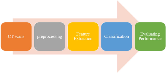
Our proposed methodology
Dataset
In our work, three CT scans datasets are used [21, 33, 35]. In Zaid [35] there are two types of images: 4001 positive CT (pCT) and 9979 negative CT (nCT) images. In our work, we use the 4001 positive CT (pCT) images but there are a lot of repetitions in the images, as well as we used the images that have full lungs by removing the upper and lower slices in the preprocessing step. The number of scans used from this dataset is 299 CT scans. In Yang et al. [33] there are 349 COVID-19 CT images and 463 non-COVID-19 CTs. We use all the COVID-19 CT images and 250 images from non-COVID-19 CTs. In Plameneduardo [21] there are 1252 CT positive scans and 1230 CT negative scans. We used 1108 positive CT scans. So, the total number of our dataset is 250 non-COVID-19 scans and 1801 COVID-19 scans.
Image preprocessing
In our work, we do two preprocessing steps on the dataset: the removing step and the cropping step. Any CT image produces 20–30 slices from the upper part of the chest to the lower part. We removed the slices that contain the upper and lower part and keep the slices that contain the complete lung regions in the removing step. In the cropping step, we crop the lung regions only and delete any surrounded regions. This step is the most difficult because not all the images have the same position of the lung. So, we did multiple cropping steps to have the best results. Figure 2 shows some samples from the removing and the cropping step.
Fig. 2.

Samples from the removing step (upper and lower parts are removed; full regions remain) and Samples from the cropping step
Feature extraction
Feature Extraction is one of the most important step in the COVID-19 classification and detection. In our work, we use 16 features to detect the stage of infection. These features are the ratio of white regions of lesions to white regions of the lung (Ratio of Infection) [22], global statistical texture features, GLCM and GLRLM texture features [3, 17, 25].
Ratio of infection feature
Figure 3 shows our proposed approach to extracting Ratio of Infection feature [22]. In the masking lung step, we increase the intensity values of image by imadjust function in MATLAB. Then, we create a binary image using Otsu’s method which convertes all values above a global threshold with 1 s and all other values with 0 s. Next, we erode the binary image using disk structuring element to mask the lung. We complement the mask. Finally, we fill the holes in the lung area. After we masked the lungs, we calculate the white regions in the image.
Fig. 3.

Ratio of Infection extraced feature step
In the masking lesions step. First, we feedback the segmented lung by multiplying the original image by the masked image. Then, we increase the intensity values of image by imadjust function in MATLAB. We erode the binary image using disk structuring element to mask the lung. We segment the lesions that are greater than the thresholding value (150). This value is determined by experiments. After we segmented the lesions, we calculated the white regions of lesions in the image. See Fig. 4.
Fig. 4.

Samples from mild, moderate, and severe stages and the steps to extract features
We can calculate the Ratio of Infection by the following equation:
| 1 |
Statistical texture features
four statistical texture features are extracted, which are mean, standard deviation, kurtosis and skewness. These features can be calculated by the following equations:
| 2 |
| 3 |
| 4 |
| 5 |
where is the mean, s is the standard deviation and M is the number of features.
Grey level co-occurrence matrix (GLCM) and grey level run length matrix (GLRLM) texture features
GLCM and GLRLM are types of texture features which can be extracted from the histogram of each image. For GLCM, there are four features are calculated: contrast, correlation, energy, and homogeneity. For GLRLM there are seven features are calculated: run percentage (RP), gray length non-uniformity (GLN), run length non-uniformity (RLN), short run emphasis (SRE), long run emphasis (LRE), low gray-level run emphasis (LGRE) and high gray-level run emphasis (HGRE). in each GLCM and GLRLM each feature is extracted in four orientations (0, 45, 90, and 135), then the average is taken.
- Gray level co-occurrence matrix (GLCM): Four GLCM features are calculated: contrast, correlation, energy, and homogeneity [3]. We can calculate them by the following equations:
6 7 8
where: M,N are the dimensions of the image p[i, j] for i=1,2,3,,M. and j=1,2,3,,N. , are the mean and the variance of the image p[i, j].9 - Gray level run length matrix (GLRLM): Seven GLRLM features are extracted: RP, GLN, RLN, SRE, LRE, LGRE and HGRE [3]. We can calculate them by the following equations:
10 11 12 13 14 15
where: Nr,Ng are the set of different run lengths and the set of different gray levels, respectively. N is the total number of the pixels in the image, calculated by the following equation:16
pij is the (i,j) entry of the GLRLM.17
Classification
To divide the dataset into training and testing, we used 8-folds cross-validation technique. four machine learning (DT, KNN, SVM and Naïve Bayes) are used to classify the images into four stages: normal, mild, moderate, and severe stage based on the features mentioned previously, see Fig. 5.
Fig. 5.

Classification steps
K-fold cross-validation
It is a method that uses to assess the machine learning models on a limited dataset. the dataset is split into k subsets randomly. One of the fold is used in the testing and the others are used in the training. this process is repeated k times. [25].
In our work, the best value of K fold is 8. The value of the fold is determined by trial and error. We try different value of the fold and notice anyone give us the lowest error in each stage. Figures 6, 7 and 8 show different values of the fold and the value of the error for each one in each stage (mild, moderate, and severe). From the figure, eight-fold cross-validation gives the lowest error in the mild, moderate, and severe stages.
Fig. 6.
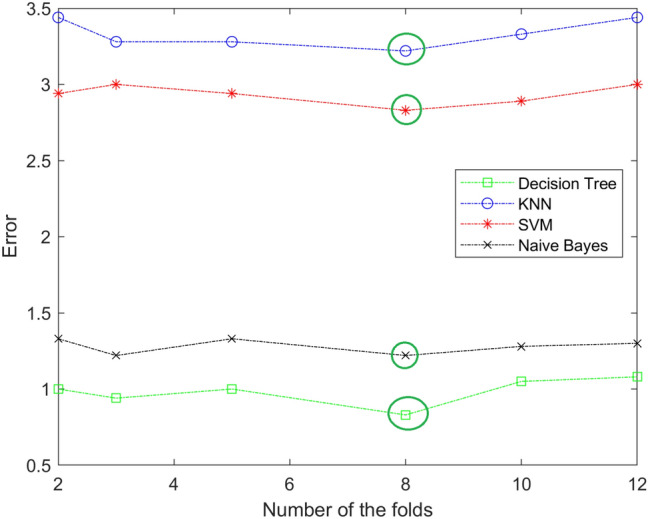
The resulting of selecting the best number of folds for KNN,SVM, and Naïve Bayes in mild stage. The best value is 8
Fig. 7.
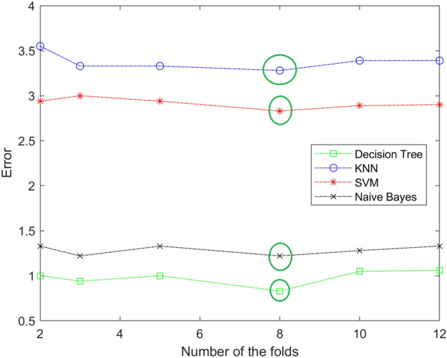
The resulting of selecting the best number of folds for DT, KNN,SVM, and Naïve Bayes in moderate stage. The best value is 8
Fig. 8.
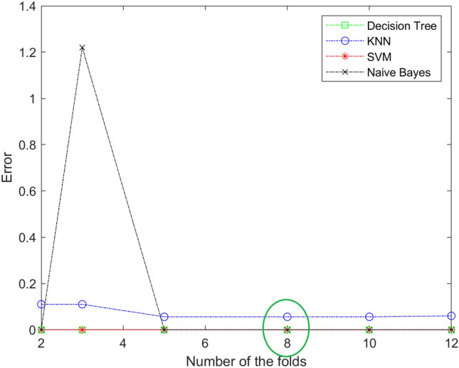
The resulting of selecting the best number of folds for DT, KNN, SVM, and Naïve Bayes in sever stage. The best value is 8
Support vector machine (SVM)
One supervised machine learning technique that may be applied to classification or regression problems is SVM. SVM is a discriminative classifier that is officially described by a separating hyperplane. An ideal hyperplane that classifies new classes is produced by the algorithm when we provide labeled training data. In two dimension, This hyperplane divides a plane into two parts with each class lying on each side. The closest points to the hyperplane from two classes that provide the greatest margin, which are used to identify the optimum line. These points are referred to as support vectors [7, 23].
K-nearest neighbor (KNN)
An approach for supervised learning that may be applied to both classification and regression is K-Nearest Neighbors (KNN). KNN attempts to predict the proper class for the test instance by computing the distance between the test instance and all labeled training examples. Then choose the K spots that are closest to the test data [8, 23].
Naive Bayes
Nave Bayes is a type of supervised machine learning that may be used to solve classification challenges. It is presumed that the existence of one feature in a class is unrelated to the presence of any other feature. It operates primarily on the probability principle, computing the odds of the test instance being assigned to each of the available class labels. The label of the test instance is determined by the largest value of these probabilities [18, 23].
Decision tree
The Decision Tree algorithm is a supervised Machine Learning Algorithm that may be used for classification and regression. Every decision tree has two nodes: the decision node and the leaf node. There are several branches at decision nodes. The leaf nodes represent the result of the decisions made to get to the point. A decision tree algorithm is so named because it begins with a root node and then branches out into multiple branches. It just asks a question and accepts a Yes/No response [23, 27].
Fine-tuning of the models
Each classifier has parameters that we fine-tune through experiments. We choose the best ones that give us the best performance. For the Decision Tree, we try three types; Fine, Medium, and Coarse. Which differ in the number of splits. 100 splits for Fine DT, 20 splits for Medium DT, and 4 splits for coarse DT. From the experiments, we find that Fine DT is the best one, which gives us the best performance. For KNN, we try three types based on the distance function type; Euclidian, Cosin, and Minkowski. Table From the experiments, we find that Weighted KNN is the best one. See table 1 explains our KNN experiments. From the experiments, we find that Weighted KNN is the best one.
Table 1.
KNN Types with their parameters
| KNN Type | distance function with value of K |
|---|---|
| Fine KNN | Euclidian distance function with K=1 |
| Weighted KNN | Euclidian distance function with K=10 |
| Coarse KNN | Euclidian distance function with K=100 |
| Cosin KNN | Cosin distance function with K=10 |
| Cubic KNN | Minkowski distance function with K=10 |
For SVM, we try four types of SVM; Cubic SVM with polynomial kernel function (order 3) and kernel scale 1, and three types of Gaussian SVM (Fine, Medium, and Coarse), all of them are Gaussian Kernel function, but they differ in kernel scale, which is 1, 4.1, and 16 for each one, respectively. From the experiments, we find that Cubic SVM is the best one.
Evaluating performance
We will investigate a number of measures to assess the efficacy of the suggested classification algorithms, including accuracy, sensitivity or recall, specificity, precision, F−score, and Receiver Operating Characteristic (ROC) area. Figure 9 depicts a 33 confusion matrix. There are four indices in any confusion matrix which are:
Fig. 9.

The confusion matrices for ML models with our proposed feature extraction method
True positive (TP): the label belongs to the class, and it is correctly predicted.
True negative (TN): the label does not belong to the class, and it is correctly predicted.
False positive (FP): the label does not belong to the class, but classifier predicted as positive.
False negative (FN): the label belongs to the class, but the classifier predicted as negative.
The performance metrics can be calculated by the following equations:
| 18 |
| 19 |
| 20 |
| 21 |
| 22 |
ROC curve is created by plotting the TP rate against the FP rate. The performance is measured by the area under the curve (AUC); the higher AUC is the best.
| 23 |
| 24 |
Experimental results and discussion
All experiments are written in MATLAB 2020a, they ran on the Windows 10 operating system of a desktop computer. The computer uses up to 8 GB of RAM, 1115 GB Hard Disk Drive, and Intel Core i3 @ 3 GHz.
The dataset (2051 scans) is classified into four stages normal with 250 CT scans, Mild with 1075 CT scans, Moderate with 434 CT scans and Severe with 292 CT scans, they rely on the description file that is found with the data set and rely on the CT findings. Then our methodology applies to each scan. 8-folds cross-validation is used to train and test our model. Figures 9, 10 and Table 4 show the results.
Fig. 10.

ROC Curves for ML models with our proposed feature extraction method
Table 4.
Performance metrics for ML models with our proposed model
| References | Number of stage | Feature extraction | Classification | Accuracy |
|---|---|---|---|---|
| Aswathy et al. [4] | 3 Stages: low, medium and high | Using ResNet-50 and ResNet-102 | using Backpropagation Neural Network | 97.3% |
| Tang et al. [28] | 2 Stages: non-severe and severe | Extracting ratio of whole lung volume to the volume of the GGO feature | using the RF | 87.5% |
| Yu et al. [34] | 2 Stages: non-severe and severe | using Inception-V3, ResNet-50, ResNet-101 and DenseNet-201 | LDA, Linear SVM, Cubic SVM and Ad boost Decision Tree | 95.2% By DenseNet-201 with Cubic SVM |
| Irmak [13] | 4 Stages: mild, moderate, severe, and critical | - | by CNN | 95.52% |
| Xiao et al. [31] | 2 Stages: non-severe and severe | - | using ResNet-34, Alex Net, VGG Net, and Dense Net | 81.9% By ResNet-34 |
| Amini and Shalbaf [3] | 4 Stages: normal, mild, moderate and severe | Extracting GLCM, GLRLM and GLSZM Features | using LDA, KNN, and RF | 90.95% |
| Our proposed model | 4 Stages: normal, mild, moderate and severe | Extracting ROI, GLCM and GLRLM features | by DT, KNN, SVM and Naive Bayes | 99% by SVM |
Figure 9 shows the confusion matrices for ML classification models DT, KNN, SVM and Naive Bayes. From the figure, the SVM model has the minimum misclassification scans (41 scans).
Figure 10 shows the ROC Curves and the AUC for each model. From the figure, the SVM has the maximum value of the AUC (99%).
Table 4 shows the performance metrics for each model in normal, mild, moderate and severe stage. From the table, SVM is the best performance in all stages. But KNN has the highest specificity in mild and moderate stages.
Table 3 shows the performance metrics for the classification models based on each feature alone (global statistical texture features, GLCM, GLRLM and ROI) features. From this step, we evaluate any feature effect on the performance of each model. From the table, we conclude that the ROI feature is the best feature and it achieves the best performance. The GLCM achieves the lowest performance (Table 2, Fig. 11).
Table 3.
The performance metrics for the classification models with Statistical, GLCM, GLRLM, and ROI Features
| ML model | Performance | Normal (%) | Mild (%) | Moderate (%) | Severe (%) | Four stages (%) |
|---|---|---|---|---|---|---|
| DT with Global | Accuracy | 91.91 | 69.16 | 96.45 | 96.81 | 91.17 |
| Sensitivity | 86.59 | 90.98 | 84.80 | 87.32 | 83.99 | |
| Specificity | 90.1 | 75.81 | 96.08 | 84.14 | 94.35 | |
| Precision | 98.22 | 100 | 100 | 100 | 85.32 | |
| DT with GLCM | Accuracy | 91.27 | 54 | 96.45 | 67.84 | 89.54 |
| Sensitivity | 86.01 | 90.23 | 81.35 | 84.2 | 71.69 | |
| Specificity | 87.13 | 70.97 | 91.47 | 69.06 | 91.68 | |
| Precision | 93.76 | 71.58 | 97.44 | 82.28 | 75.85 | |
| DT with GLRLM | Accuracy | 95.81 | 83.2 | 97.56 | 82.54 | 94.32 |
| Sensitivity | 92.44 | 93.12 | 91.7 | 92.51 | 86.39 | |
| Specificity | 92.1 | 80.88 | 95.11 | 81.63 | 95.68 | |
| Precision | 96.93 | 88.36 | 98.35 | 89.9 | 86.64 | |
| DT with ROI | Accuracy | 88.74 | 37.2 | 95.89 | 55.69 | 93.53 |
| Sensitivity | 88.10 | 93.21 | 82.48 | 85.42 | 80.14 | |
| Specificity | 98.34 | 94.93 | 99.26 | 97.17 | 94.28 | |
| Precision | 98.88 | 95.21 | 99.49 | 96.86 | 83.79 | |
| DT with all features | Accuracy | 96.39 | 96.34 | 98.1 | 100 | 97.71 |
| Sensitivity | 89.2 | 95.91 | 94.7 | 100 | 94.95 | |
| Specificity | 997.39 | 96.82 | 99.01 | 100 | 98.31 | |
| Precision | 82.59 | 97.08 | 96.25 | 100 | 93.93 | |
| KNN with Global | Accuracy | 98.29 | 94 | 98.89 | 92.16 | 95.93 |
| Sensitivity | 92.25 | 93.12 | 91.29 | 92.17 | 92.29 | |
| Specificity | 93.17 | 82.03 | 96.17 | 85.17 | 96.59 | |
| Precision | 100 | 100 | 100 | 100 | 92.37 | |
| KNN with GLCM | Accuracy | 97.56 h | 92.40 | 98.28 | 88.17 | 93.98 |
| Sensitivity | 91.91 | 92.56 | 91.19 | 92.04 | 86.31 | |
| Specificity | 90.78 | 77.42 | 94.37 | 78.69 | 95.41 | |
| Precision | 95.66 | 82.88 | 97.78 | 86.12 | 86.26 | |
| KNN with GLRLM | Accuracy | 98.59 | 95.2 | 99.06 | 93.33 | 96.47 |
| Sensitivity | 95.32 | 95.72 | 94.88 | 95.37 | 91.91 | |
| Specificity | 94.05 | 86.64 | 96.04 | 85.45 | 97.29 | |
| Precision | 97.9 | 90.07 | 99.20 | 94.95 | 92.27 | |
| KNN with ROI | Accuracy | 92.54 | 86 | 93.45 | 64.56 | 95.22 |
| Sensitivity | 91.71 | 88.84 | 94.88 | 95.02 | 90.87 | |
| Specificity | 97.95 | 94.47 | 98.89 | 95.79 | 96.67 | |
| Precision | 98.68 | 94.18 | 99.43 | 96.49 | 87.97 | |
| KNN with all features | Accuracy | 98.83 | 96.44 | 96.78 | 99.95 | 98 |
| Sensitivity | 94.8 | 96.74 | 92.4 | 99.66 | 95.9 | |
| Specificity | 99.66 | 99.39 | 96.11 | 97.96 | 98.36 | |
| Precision | 95.56 | 96.47 | 92.4 | 100 | 96.11 | |
| SVM with Global | Accuracy | 87.76 | 18.09 | 99 | 48.57 | 87.66 |
| Sensitivity | 84.15 | 95.53 | 85.24 | 89.46 | 74.43 | |
| Specificity | 86.35 | 84.1 | 96.24 | 86.9 | 95.12 | |
| Precision | 92.39 | 100 | 100 | 100 | 81.23 | |
| SVM with GLCM | Accuracy | 94.54 | 64.4 | 98.18 | 82.99 | 93.49 |
| Sensitivity | 90.39 | 94.51 | 84.99 | 87.29 | 80.29 | |
| Specificity | 92.35 | 81.08 | 94.87 | 81.26 | 94.18 | |
| Precision | 96.68 | 81.16 | 98.7 | 91.15 | 85.61 | |
| SVM with GLRLM | Accuracy | 98.24 | 90 | 99.39 | 95.34 | 96.42 |
| Sensitivity | 95.22 | 97.3 | 92.93 | 93.81 | 90.46 | |
| Specificity | 94.54 | 86.87 | 96.6 | 87.27 | 97.06 | |
| Precision | 97.66 | 87.67 | 99.32 | 95.52 | 92.59 | |
| SVM with ROI | Accuracy | 98.29 | 88.4 | 99.83 | 98.66 | 98.42 |
| Sensitivity | 98.2 | 99.44 | 97.12 | 97.45 | 95.26 | |
| Specificity | 98.39 | 96.98 | 98.95 | 96.09 | 98.82 | |
| Precision | 98.78 | 96.23 | 99.37 | 96.23 | 97.11 | |
| SVM with all features | Accuracy | 99.12 | 98.24 | 98.73 | 99.9 | 99 |
| Sensitivity | 96.4 | 98.6 | 96.08 | 100 | 97.77 | |
| Specificity | 99.5 | 97.85 | 99.44 | 99.89 | 99.17 | |
| Precision | 96.4 | 98.06 | 97.89 | 99.32 | 97.92 | |
| Naive Bayes with Global | Accuracy | 81.91 | 68.4 | 83.79 | 36.93 | 87.42 |
| Sensitivity | 79.18 | 72 | 87.09 | 86 | 77.27 | |
| Specificity | 88.39 | 68.66 | 93.94 | 75.25 | 91.2 | |
| Precision | 100 | 100 | 100 | 100 | 74.55 | |
| Naive Bayes with GLCM | Accuracy | 87.03 | 28 | 95.22 | 44.87 | 82.18 |
| Sensitivity | 77.28 | 94.05 | 58.81 | 71.55 | 48 | |
| Specificity | 78.99 | 24.42 | 93.63 | 50.72 | 84.93 | |
| Precision | 85.42 | 45.55 | 92.04 | 48.72 | 53.96 | |
| Naive Bayes with GLRLM | Accuracy | 92.54 | 74.8 | 95 | 67.51 | 90.66 |
| Sensitivity | 89.66 | 89.02 | 90.37 | 91.06 | 76.13 | |
| Specificity | 87.13 | 79.72 | 89.12 | 66.28 | 93.23 | |
| Precision | 93.32 | 60.96 | 98.69 | 88.5 | 78.35 | |
| Naive Bayes with ROI | Accuracy | 98.73 | 89.6 | 100 | 100 | 98.27 |
| Sensitivity | 93.1 | 98.42 | 97.75 | 97.96 | 94.97 | |
| Specificity | 97.66 | 97 | 97.84 | 92.32 | 98.7 | |
| Precision | 98.59 | 94.86 | 99.2 | 95.19 | 96.37 | |
| Naive Bayes with all features | Accuracy | 91.18 | 89.52 | 96.59 | 100 | 94.32 |
| Sensitivity | 78 | 86.88 | 91.47 | 100 | 89.09 | |
| Specificity | 93 | 92.42 | 97.96 | 100 | 95.85 | |
| Precision | 60.75 | 92.66 | 92.33 | 100 | 86.43 |
Bold value indicates the best performances
Table 2.
Performance metrics for ML models with our proposed model
| ML | Stage | Accuracy (%) | Sensitivity (%) | Specificity (%) | Precision (%) | F-score (%) |
|---|---|---|---|---|---|---|
| Decision Tree | Normal | 96.39 | 89.2 | 97.39 | 82.59 | 85.77 |
| Mild | 96.34 | 95.91 | 96.82 | 97.08 | 96.99 | |
| Moderate | 98.1 | 94.7 | 99.01 | 96.25 | 95.47 | |
| Severe | 100 | 100 | 100 | 100 | 100 | |
| KNN | Normal | 98.83 | 94.8 | 99.66 | 95.56 | 95.18 |
| Mild | 96.44 | 96.74 | 99.39 | 96.47 | 96.61 | |
| Moderate | 96.78 | 92.40 | 96.11 | 92.4 | 92.40 | |
| Severe | 99.95 | 99.66 | 97.96 | 100 | 99.83 | |
| SVM | Normal | 99.12 | 96.4 | 99.5 | 96.4 | 96.4 |
| Mild | 98.24 | 98.6 | 97.85 | 98.06 | 98.33 | |
| Moderate | 98.73 | 96.08 | 99.44 | 97.89 | 96.98 | |
| Severe | 99.9 | 100 | 99.89 | 99.32 | 99.66 | |
| Naive Bayes | Normal | 91.18 | 78 | 93 | 60.75 | 68.3 |
| Mild | 89.52 | 86.88 | 92.42 | 92.66 | 89.68 | |
| Moderate | 96.59 | 91.97 | 97.96 | 92.33 | 91.9 | |
| Severe | 100 | 100 | 100 | 100 | 100 |
Fig. 11.

Performance metrics for ML models with our proposed model
Figure 12 shows the average accuracy of four stages for four models based on each feature.
Fig. 12.

The average accuracy of four stages for four models based on each feature
Comparing with state-of-arts models results and discussion
Table 4 shows a comparison between our work and other studies in a classification of severity of COVID-19 CT scans. From it, our model achieves higher accuracy than other existed models. Our model is reliable, high speed, and robust. So, we can rely on it to determine the degree of infection and provide the appropriate dose during the treatment period.
Conclusions and future works
We developed a systematic technique for COVID-19 identification, lung and lesion segmentation, and patient severity rating using CT scans in this thesis. We presented and analyzed numerous cutting-edge segmentation networks in order to discover the top performing machine learning algorithms. The presented scheme and models obtained exquisite performance levels in segmentation, classification, and infection quantification. Nevertheless, we have proposed a simple, reliable and automatic model to detect the severity of COVID-19 based on the CT scans to three stages: mild, moderate, and severe stage. This model based on finding the ratio of infection ( ratio of the lesions area to the lung area), global statistical, GLCM, and GLRLM features. Three ML algorithms are used to classify CT scans (DT, KNN, SVM, and Naïve Bayes). From experiments, our model achieves 99.12% of accuracy for normal stage, 98.24% of accuracy for mild stage, 98.73% of accuracy for moderate stage and 99.9% of accuracy for severe stage by SVM model. Our model achieves better performance than state-of-arts models also. To summarize, computer-aided detection and quantification provides a reliable, simple, and cost-effective technique of diagnosing COVID-19 cases.
Our model based on CT scans only, as future works, we will consider other factors that effect on the COVID-19 severity such as background disease (like diabetes, etc.), blood test vital, and demographic. these features have useful information can be used to increase the accuracy of our model. As well as we will increase the number of datasets. We will add other machine learning models.
Biographies
Zaid Albataineh
received the B.S. degree in electrical engineering from the Yarmouk University, Irbid, Jordan, in 2006, and received the M.S. degree in the communication and electronic engineering from the Jordan University of Science and Technology JUST, Irbid, Jordan, in 2009. He received the Ph.D. degree in electrical and computer engineering department, Michigan State University (MSU), USA, in 2014. His research interests include Blind Source Separation, Independent Component analysis, Nonnegative matrix Factorization, Wireless Communication, DSP Implementation, VLSI, Analog Integrated Circuit and RF Integrated Circuit.
Fatima Aldrweesh
was born in Irbid, Jordan. B.S. at Yarmouk University, Jordan 2016, Electronics Engineering, Msc in Computer Engineering, 2022, Yarmouk University. Currently, her research interests include machine learning, deep learning and image processing.
Mohammad A. Alzubaidi
is an Associate Professor of computer engineering at Yarmouk University, Jordan. He received his PhD degree in Computer Science and Engineering from the Ira Fulton School of Engineering at Arizona State University in 2012. His research areas are medical imaging perception and understanding, computer vision and pattern recognition, assistive technology, and machine learning.
Author contributions
ZA and FA wrote the main manuscript text and prepared all figures. All authors reviewed the manuscript.
Funding
Not applicable.
Data availability
The data presented in this study are available on request from the corresponding author.
Declarations
Conflict of interest
The authors declare no conflict of interest.
Footnotes
Publisher's Note
Springer Nature remains neutral with regard to jurisdictional claims in published maps and institutional affiliations.
Contributor Information
Zaid Albataineh, Email: zaid.bataineh@yu.edu.jo.
Fatima Aldrweesh, Email: fatimaaldrweesh92@gmail.com.
Mohammad A. Alzubaidi, Email: maalzubaidi@yu.edu.jo
References
- 1.Alyasseri ZAA. Review on COVID-19 diagnosis models based on machine learning and deep learning approaches. Expert. Syst. 2022;39(3):e12759. doi: 10.1111/exsy.12759. [DOI] [PMC free article] [PubMed] [Google Scholar]
- 2.Alzubaidi MA, et al. A novel computational method for assigning weights of importance to symptoms of COVID-19 patients. Artif. Intell. Med. 2021;112:102018. doi: 10.1016/j.artmed.2021.102018. [DOI] [PMC free article] [PubMed] [Google Scholar]
- 3.Amini N, Shalbaf A. Automatic classification of severity of COVID-19 patients using texture feature and random forest based on computed tomography images. Int. J. Imaging Syst. Technol. 2022;32(1):102–110. doi: 10.1002/ima.22679. [DOI] [PMC free article] [PubMed] [Google Scholar]
- 4.Aswathy AL, Hareendran A, Vinod Chandra SS. COVID-19 diagnosis and severity detection from CT-images using transfer learning and back propagation neural network. J. Infect. Public Health. 2021;14(10):1435–1445. doi: 10.1016/j.jiph.2021.07.015. [DOI] [PMC free article] [PubMed] [Google Scholar]
- 5.Al-Azawi RJ, et al. Efficient classification of COVID-19 CT scans by using q-transform model for feature extraction. PeerJ Comput. Sci. 2021;7:e553. doi: 10.7717/peerj-cs.553. [DOI] [Google Scholar]
- 6.Calvo C, et al. Recommendations on the clinical management of the COVID-19 infection by the new coronavirus SARS-CoV2. Spanish Paediatric Association working group. Anales de Pediatríéa (English Edition) 2020;92(4):241–e1. doi: 10.1016/j.anpede.2020.02.002. [DOI] [PMC free article] [PubMed] [Google Scholar]
- 7.Cervantes J, et al. A comprehensive survey on support vector machine classification: applications, challenges and trends. Neurocomputing. 2020;408:189–215. doi: 10.1016/j.neucom.2019.10.118. [DOI] [Google Scholar]
- 8.Coomans D, Massart DL. Alternative k-nearest neighbour rules in supervised pattern recognition: part 1. k-Nearest neighbour classification by using alternative voting rules. Anal. Chim. Acta. 1982;136:15–27. doi: 10.1016/S0003-2670(01)95359-0. [DOI] [Google Scholar]
- 9.Ding X, et al. Chest CT findings of COVID-19 pneumonia by duration of symptoms. Eur. J. Radiol. 2020;127:109009. doi: 10.1016/j.ejrad.2020.109009. [DOI] [PMC free article] [PubMed] [Google Scholar]
- 10.Feng W, et al. Molecular diagnosis of COVID-19: challenges and research needs. Anal. Chem. 2020;92(15):10196–10209. doi: 10.1021/acs.analchem.0c02060. [DOI] [PubMed] [Google Scholar]
- 11.Flor LS, et al. Quantifying the effects of the COVID-19 pandemic on gender equality on health, social, and economic indicators: a comprehensive review of data from March, 2020, to September, 2021. Lancet. 2022 doi: 10.1016/S0140-6736(22)00008-3. [DOI] [PMC free article] [PubMed] [Google Scholar]
- 12.Gomes R, et al. A comprehensive review of machine learning used to combat COVID- 19. Diagnostics. 2022;12(8):1853. doi: 10.3390/diagnostics12081853. [DOI] [PMC free article] [PubMed] [Google Scholar]
- 13.Irmak E. COVID-19 disease severity assessment using CNN model. IET Image Proc. 2021;15(8):1814–1824. doi: 10.1049/ipr2.12153. [DOI] [PMC free article] [PubMed] [Google Scholar]
- 14.Iwanaga J, et al. A review of anatomy education during and after the COVID-19 pandemic: revisiting traditional and modern methods to achieve future innovation. Clin. Anat. 2021;34(1):108–114. doi: 10.1002/ca.23655. [DOI] [PMC free article] [PubMed] [Google Scholar]
- 15.Kim H, Hong H, Yoon SH. Diagnostic performance of CT and reverse transcriptase-polymerase chain reaction for coronavirus disease 2019: a meta-analysis. Radiology. 2020 doi: 10.1148/radiol.2020201343. [DOI] [PMC free article] [PubMed] [Google Scholar]
- 16.Mahesh B. Machine learning algorithms—a review. Int. J. Sci. Res. 2020;9:381–386. [Google Scholar]
- 17.Mohanty AK, et al. Texture-based features for classification of mammograms using decision tree. Neural Comput. Appl. 2013;23(3):1011–1017. doi: 10.1007/s00521-012-1025-z. [DOI] [Google Scholar]
- 18.Murphy KP, et al. Naive bayes classifiers. Univ. Br. Columbia. 2006;18(60):1–8. [Google Scholar]
- 19.Padhan R, Prabheesh KP. The economics of COVID-19 pandemic: a survey. Econ. Anal. Policy. 2021;70:220–237. doi: 10.1016/j.eap.2021.02.012. [DOI] [PMC free article] [PubMed] [Google Scholar]
- 20.Pan F, et al. Time course of lung changes at chest CT during recovery from coronavirus disease 2019 (COVID-19) Radiology. 2020;295(3):715–721. doi: 10.1148/radiol.2020200370. [DOI] [PMC free article] [PubMed] [Google Scholar]
- 21.Plameneduardo: SARS-COV-2 Ct-Scan Dataset. https://www.kaggle.com/datasets/ plameneduardo/sarscov2-ctscan-dataset (2020)
- 22.Qiblawey Y, et al. Detection and severity classification of COVID-19 in CT images using deep learning. Diagnostics. 2021;2021(11):893. doi: 10.3390/diagnostics11050893. [DOI] [PMC free article] [PubMed] [Google Scholar]
- 23.Ray, S.: A quick review of machine learning algorithms. In: 2019 International conference on machine learning, big data, cloud and parallel computing (COMITCon). IEEE, pp. 35–39 (2019)
- 24.Reuge N, et al. Education response to COVID 19 pandemic, a special issue proposed by UNICEF: editorial review. Int. J. Educ. Dev. 2021;87:102485. doi: 10.1016/j.ijedudev.2021.102485. [DOI] [PMC free article] [PubMed] [Google Scholar]
- 25.Sharda, R., Delen, D., Turban, E.: Business intelligence analytics and data science: a managerial perspective, 4th edn. Pearson (2017)
- 26.Shi H, et al. Radiological findings from 81 patients with COVID-19 pneumonia in Wuhan, China: a descriptive study. Lancet. Infect. Dis. 2020;20(4):425–434. doi: 10.1016/S1473-3099(20)30086-4. [DOI] [PMC free article] [PubMed] [Google Scholar]
- 27.Srivastava A, et al. High Performance Data Mining. Cham: Springer; 1999. Parallel formulations of decision-tree classification algorithms; pp. 237–261. [Google Scholar]
- 28.Tang, Z., et al.: Severity assessment of coronavirus disease 2019 (COVID-19) using quantitative features from chest CT images. arXiv preprint arXiv:2003.11988 (2020)
- 29.Wang K, et al. Imaging manifestations and diagnostic value of chest CT of coronavirus disease 2019 (COVID-19) in the Xiaogan area. Clin. Radiol. 2020;75(5):341–347. doi: 10.1016/j.crad.2020.03.004. [DOI] [PMC free article] [PubMed] [Google Scholar]
- 30.WHO: World Health Organization. WHO announces COVID-19 outbreak pandemic. https://www.who.int/emergencies/diseases/novel-coronavirus-2019 (2019)
- 31.Xiao L, et al. Development and validation of a deep learning-based model using computed tomography imaging for predicting disease severity of coronavirus disease 2019. Front. Bioeng. Biotechnol. 2020;8:898. doi: 10.3389/fbioe.2020.00898. [DOI] [PMC free article] [PubMed] [Google Scholar]
- 32.Yang H, et al. Application of machine learning methods in bioinformatics. AIP Conf. Proc. 2018;1967(1):040015. doi: 10.1063/1.5039089. [DOI] [Google Scholar]
- 33.Yang, X., et al.: COVID-CT-dataset: a CT scan dataset about COVID-19. arXiv preprint arXiv:2003.13865 (2020)
- 34.Yu Z, et al. Rapid identification of COVID-19 severity in CT scans through classification of deep features. Biomed. Eng. Online. 2020;19(1):1–13. doi: 10.1186/s12938-020-00807-x. [DOI] [PMC free article] [PubMed] [Google Scholar]
- 35.Zaid, B., Abu, A.: CT scans for COVID-19 classification. https://www.kaggle.com/ datasets/azaemon/preprocessed-ct-scans-for-covid19 (2020)
- 36.Zhou S, et al. Imaging features and evolution on CT in 100 COVID-19 pneumonia patients in Wuhan, China. Eur. Radiol. 2020;30(10):5446–5454. doi: 10.1007/s00330-020-06879-6. [DOI] [PMC free article] [PubMed] [Google Scholar]
- 37.Zhu J, et al. Deep transfer learning artificial intelligence accurately stages COVID-19 lung disease severity on portable chest radiographs. PLoS ONE. 2020;15(7):e0236621. doi: 10.1371/journal.pone.0236621. [DOI] [PMC free article] [PubMed] [Google Scholar]
Associated Data
This section collects any data citations, data availability statements, or supplementary materials included in this article.
Data Availability Statement
The data presented in this study are available on request from the corresponding author.