

Abstract
Water often plays a key role in mediating protein-ligand interactions. Understanding contributions from active-site water molecules to binding thermodynamics of a ligand is important in predicting binding free energies for ligand optimization. In this work, we tested a nonequilibrium switching method for absolute binding free energy calculations on water molecules in binding sites of 13 systems. We discuss the lessons we learned about identified issues that affected our calculations and ways to address them. This work fits with our larger focus on how to do accurate ligand binding free energy calculations when water rearrangements are very slow, such as rearrangements due to ligand modification (as in relative free energy calculations) or ligand binding (as in absolute free energy calculations). The method studied in this work can potentially be used to account for limited water sampling via providing endpoint corrections to free energy calculations using our calculated binding free energy of water.
Graphical Abstract
2. Introduction
Understanding the role of water molecules in a protein binding site can facilitate designing ligands with improved binding affinity. When a ligand modification displaces a bound water in the binding site, this can contribute to binding due to an increase in entropy associated with water liberation. However, the overall ligand binding affinity depends on whether the modified ligand can make favorable interactions with the protein and compensate the enthalpy loss of water displacement. Thus, understanding the energetics of water molecules in a binding site is important to optimizing ligand binding in drug discovery.
Proper treatment of buried water molecules in a protein binding site is important and challenging for robust binding free energy calculations. Molecular dynamics (MD) simulations can account for the water thermodynamics in protein-ligand binding free energy calculations if water molecules are adequately sampled throughout the simulations. However, the time required for water rearrangement in the binding site upon a ligand binding may be beyond the typical timescales of MD simulations (e.g., ns or μs). Particularly, in relative binding free energy calculations to compare binding potency between two ligands, researchers commonly transform one ligand (ligand A) into another (ligand B) in both bound state and in solution via a series of non-physical intermediate states (called “alchemical“ states, created through use of a scaling factor λ).1 In the case where morphing ligand A into ligand B leads to water displacement or more room for extra water molecules, the accuracy of relative binding free energy (RBFE) calculations will be impaired if we do not sample such water rearrangement correctly.2–4 Even though RBFE simulations are normally done on structurally similar ligands, these ligands may still have differences in water placement in the binding site,5–8 making water sampling a common challenge in these simulations.
Given the importance and difficulty of water sampling in binding free energy calculations, a variety of methods9–21 have been developed to advance the knowledge of water molecule placement and energetics in binding sites, as reviewed previously.22,23 Some of these methods have shown promise in sampling water rearrangement on ligand binding24 and have been integrated into a popular RBFE workflow.18,19
There are two approaches to solve the water sampling issue in RBFE calculations. One straightforward approach, as just described, is to mix the water sampling into RBFE calculations.18,19 The advantage of this approach is its simplicity – a single RBFE calculation computes the true free energy for modifying the ligand, including effects of any water rearrangement or displacement. However, sampling may not be adequate; this can mix sampling problems associated with protein and water rearrangements with those associated with the intermediate alchemical state, potentially creating somewhat of a combinatorial explosion of sampling challenges, any one of which may make adequate sampling extremely difficult. In previous work, we found that enhanced methods for water sampling (grand canonical Monte Carlo (GCMC), nonequilibrium candidate Monte Carlo (NCMC) and normal MD) cannot successfully capture water rearrangement in all the systems studied, even in the absence of coupling with binding free energy calculations.24
Another approach involves separation of states,25 seeking to separate estimation of contributions from water and protein rearrangement from calculation of binding, then accounting for these various contributions separately (e.g. through end point corrections). For example, in Figure 1 we show a typical thermodynamic cycle for relative binding free energy calculations of ligand A (blue triangle) and ligand B (green rectangle). Suppose that there is one water molecule in the binding site when ligand B is present (green rectangle) and the water molecule mediates the interaction between the receptor and ligand B and is absent in ligand A bound state. In order to get a correct binding thermodynamic estimate, this water rearrangement needs to be captured in simulations when morphing ligand A into ligand B in the binding site. That said, if this water motion is not well sampled during RBFE simulations, instead of obtaining ΔGA→B(complex,wat), we end up getting ΔGA→B(complex). Then we get incorrect binding free energy difference between ligand A and B when we use the difference between ΔGA→B(solution) and ΔGA→B(complex) (instead of ΔGA→B(complex,wat)). However, we can correct this estimate by running additional simulations to account for the free energy cost of binding of this water molecule with ligand B (ΔGwat), while also capturing any other associated protein/ligand motions. Then we can use ΔGA→B(solution), ΔGA→B(complex) and ΔGwat to get the correct binding free energy difference between ligand A and B.
Figure 1:
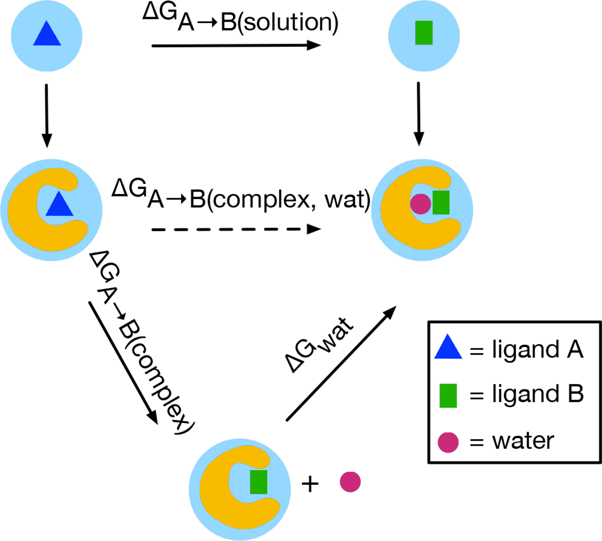
Thermodynamic cycle for computing relative binding free energy using MD simulations. ΔGA→B(solution) represents the free energy cost of morphing ligand A (blue triangle) into ligand B (green rectangle) in solution. ΔGA→B(complex,wat) represents the free energy cost of morphing ligand A into B in the bound state where the water (red circle) is in the binding site. The dashed line indicates it is difficult to calculate this free energy cost because of the extra water molecule in the binding site for ligand B. ΔGA→B(complex) is similar to ΔGA→B(complex,wat) but the water is not in the binding site. ΔGwat is the binding free energy for the water. Changing from ligand A to ligand B makes room for one water (rose red circle) that mediates the interaction between the receptor and ligand B. If the water rearrangement is not sampled adequately upon transformation of ligand A into ligand B, we obtain incorrect binding thermodynamics (incorrect ΔGA→B(complex,wat)). Instead of ΔGA→B(complex,wat), we end up getting ΔGA→B(complex) from simulations. However, we can correct this calculation by accounting for the free energy of inserting this water molecule into the binding site of ligand B (ΔGwat).
This approach will work best when we know in advance the number and location of water molecules in the binding site for individual ligands (e.g., from crystal structures or prior study via enhanced sampling methods or long MD with sufficient sampling to recover true water occupancy details). Here our focus is not on determining this information; for the purposes of the present study, we assume that the expected water structure is already known experimentally or from prior computational study.
We expect this approach may work well on cases of isolated waters or for water networks which can be addressed one water at a time, but this approach is not expected to handle complex water networks well, and a separation of states approach may not be well suited to such cases.
Suppose we know, from available crystal structures and/or long MD simulations, that ligand A and B bind with a different number of water molecules in the binding site. Suppose we already know the water rearrangement is too slow to be captured in binding free energy calculations (e.g., based on prior simulations), even if they are done with enhanced sampling like GCMC. How, then, can we do the correct binding free energy calculation for the transformation of ligand A to B? The motivation of this work is to develop an approach that could be used in this scenario.
The advantage of treating water sampling problems separately from the free energy calculation, via an endpoint correction, is with such an approach we would avoid mixing the protein-ligand and water sampling issues with the need to sample across all alchemical intermediate states for the ligand transformation. In cases where water does not pose sampling issues in RBFE calculations, we would not need this additional calculation of water binding. That said, this approach will work best when we already know the relevant water location(s) for any waters which are difficult to sample in free energy calculations.
To test whether this idea could work in practice, we first need to develop an approach to efficiently and accurately compute the binding free energy of buried water in the binding site, which is the goal of this work. We only focus on one water molecule in the binding site instead of a water network. In the fully general case, multiple correlated waters may rearrange on binding, introducing additional complexities. However, even the present problem has not yet been adequately treated in prior work.
Particularly, we are interested in applying a non-equilibrium switching (NES) based approach to achieve our goal since NES approaches have shown success in both absolute and relative binding free energy calculations for ligand binding.26–30
The main goal of this work is to develop an NES based approach to accurately and efficiently calculate the absolute binding free energy of a water molecule in the binding site. Furthermore, we seek to determine whether there are any issues that may impair the performance of this approach. If so, we want to determine how to fix such issues to allow for more robust calculations. To address these points, we first test this approach in 13 target systems for which the computed binding free energy of selected water molecules in the binding site was reported in a previous computational study.17 We analyze our simulations and detect sampling issues that affect the accuracy and convergence of our calculations. We also propose and validate solutions of these problems.
3. METHODS
3.1. Conceptual framework
Free energy is a state function and is independent of the pathway used to connect the two end states (e.g., bound and unbound states). Instead of directly simulating the computationally demanding events (e.g., binding/unbinding), the binding free energy of the target water molecule can be computed via a thermodynamic cycle through summation of free energy changes along the cycle. Figure 2 shows the thermodynamic cycles to compute the binding free energy of a water molecule (ΔGbinding) using the method presented in this work.
Figure 2:
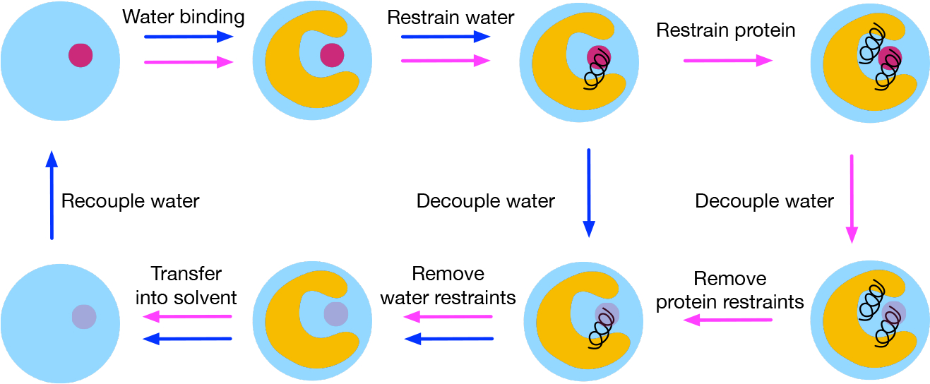
Thermodynamic cycles for computing water binding free energies. The cycle with blue arrows represent the standard cycle; the cycle with magenta arrows are used when restraints on the protein are applied to prevent binding site collapses in simulations. ”Water binding” edge: Water binds to the protein and calculating the associated free energy cost (or benefit) is the goal of this work. ”Restrain water” edge: The water is restrained to a position using a harmonic distance restraint. ”Decouple water” edge (blue arrow): The water is decoupled in the binding site by turning off its intermolecular electrostatic and van der Waals (vdW) interactions. ”Remove water restraints” edge: The harmonic distance restraint is released for the decoupled water molecule in the binding site. ”Transfer into solvent” edge: The decoupled water is transferred to the bulk solvent. ”Recouple water” edge: The water is recoupled in the bulk solvent by turning on its intermolecular electrostatic and vdW interactions. ”Restrain protein” edge: The protein binding site is restrained using position restraints. ”Decouple water” edge (magenta arrow): The water is decoupled in the binding site while it is restrained and the protein binding site is also restrained. ”Remove protein restraints” edge: The protein restraints are released while the water is still restrained.
We use NES simulations to compute the contributions of decoupling the alchemical water in the binding site and recoupling it in the bulk solvent through turning off/on its intermolecular electrostatic and van der Waals (vdW) interactions (Figure 2). We implement a single harmonic distance restraint between the oxygen atom on the alchemical water and a virtual site defined by using two heavy atoms on the protein. This restraint limits the volume available to the non-interacting alchemical water and thus helps our calculations converge faster. We need to release this harmonic restraint on the alchemical water for both the interacting and non-interacting state (red and transparent circle in Figure 2). The restraint is released analytically for the decoupled alchemical water. For the interacting state, we run simulations at two end states (unrestrained vs. restrained) and use the Bennett acceptance ratio (BAR)31 to estimate the free energy difference.
In some cases (such as in BPTI), when the alchemical water molecule is not interacting in the binding site (fully decoupled), the protein binding site collapses in simulations. So we use a different thermodynamic cycle (extra magenta arrows in Figure 2) to help avoid states where it is necessary for the protein to collapse. We add additional position restraints on atoms in protein binding site residues and decouple the restrained water in the restrained binding site using NES simulations as we did in the standard cycle (blue arrows in Figure 2). The free energy cost of applying these position restraints is calculated as the free energy difference between the two end states (restrained protein versus non-restrained protein). In order to obtain a reliable estimate of this free energy, multiple intermediate λ states (λ is used to scale the restraint strength) are deployed for sufficient phase space overlap between the two end states. The multistate Bennett acceptance ratio (MBAR)32 estimator is used to estimate the free energy difference.
The non-equilibrium switching protocol samples the alchemical path between two physical end states in fast transitions without reaching equilibrium at intermediate state as required in equilibrium approaches. The work done on the system for forward (PF(W)) and backward transformation (PR(−W)) is related to the free energy difference between the two end states (ΔG) through the Crooks fluctuation theorem:33–35
| (1) |
PF(W) and PR(−W) are the probability distribution of forward and reverse work values. When transitions are performed for only one direction (forward or backward), the Crooks fluctuation theorem reduces to the Jarzynski equality.36,37 It has been shown that the bidirectional approach (Crooks fluctuation theorem) converges faster than the exponential averaging method (Jarzynski equality).38
In this work the Crooks fluctuation theorem is solved for ΔG with the BAR estimator31 by numerically solving the following equation:
| (2) |
Here, nf and nr are the number of transitions in the forward and reverse direction. The non-equilibrium work along the bidirectional path (Wf and Wr) is obtained by accumulating the energy changes as the coupling parameter (λ) is changed during the transition:
| (3) |
3.2. Selected Targets.
We selected targets from a previous study which focused on classifying conserved and displaceable water molecules in the binding site of protein-ligand systems via absolute binding free energy calculations.17 We picked those systems which had one target water molecule in the binding site or in which the target water molecule is not interacting with other water molecules in the binding site (based on the crystal structures). These selected cases are proteins where specific water molecules make contact with the ligand: HIV-1 protease, trypsin, factor Xa (FXa), and scytalone dehydratase. For each protein target, we selected 3 ligands and the buried water molecule of interest exists in the same location in all of these systems. The previously computed binding free energy of the target water for each protein target differs by more than 1 kcal/mol between selected ligands (scytalone dehydratase is an exception, more details below). We also included a BPTI system in this work which had been used as a validation system in previous work focusing on binding free energy calculations of water molecules.17 In total, we studied 13 systems (and calculated binding free energies for 13 water molecules) in this work. Figure 3 shows the location of the target water site in each protein target and the relevant Protein Data Bank (PDB) IDs.
Figure 3:
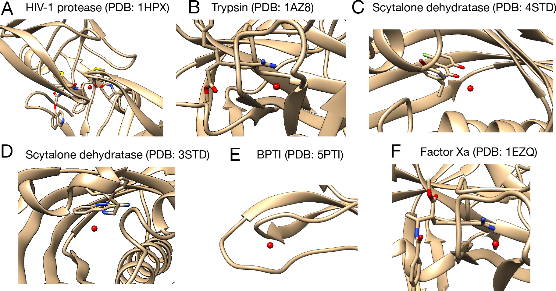
Target protein systems studied in this work and the corresponding water sites (red spheres). For each protein target we selected three ligands and we show one for each target here, along with the associated PDB IDs. The BPTI system does not have a ligand. The complete list of simulated systems and their PDB IDs are: (A)HIV-1 protease (PDB: 1HPX, 1EC0, 1EBW) (B) Trypsin (PDB: 1AZ8, 1C5T, 1GI1) (C) Scytalone dehydratase (PDB: 4STD, 7STD) (D) Scytalone dehydratase (PDB: 3STD) (E) Factor Xa (PDB: 1EZQ, 1LPG, 1F0S) (F) BPTI (PDB: 5PTI) Two different water sites were studied in scytalone dehydratase.
3.3. Simulation Details.
To prepare our simulations, we first downloaded the protein-ligand structures from the Protein Data Bank website39 (https://www.rcsb.org). We used pdbfixer 1.6 (https://github.com/openmm/pdbfixer) to add the missing heavy atoms to the receptor. Then, the PROPKA algorithm40,41 on PDB2PQR web server42 was used to set protein residue protonation states as appropriate for the pH values used for crystallography in each case. For the HIV-1 protease systems, the protonation states of the two aspartic acids in the binding site were known from previous work so we decided to use the same protonation states as the literature.17 The pKa values of the ligands were eestimated using Chemicalize (ChemAxon, https://www.chemaxon.com). The AMBER ff99 force field43 was used for protein parameterization in conjunction with the TIP4P water model.44 The ligand was parameterized using Open Force Field version 1.2.1 (codenamed “Parsley”)45,46 and AM1-BCC charges.47
3.3.1. Minimization and equilibration
All MD simulations were performed using GROMACS 2020.4.48 A time step of 2 fs was used in MD simulations. Long-range electrostatics were calculated using Particle Mesh Ewald (PME)49,50 with nonbonded cutoffs of 10 Å. Each system was simulated at 298.15 K. Simulations of different edges in Figure 2 followed the same general procedure for minimization and equilibration: the system was first minimized using steepest descent for 5000 steps, then equilibrated in the NVT ensemble for 10 ps, using the stochastic dynamics integrator and an inverse friction constant of 2 ps. A longer equilibration stage was performed in the NPT ensemble for 100 ps, with settings otherwise the same, except it used a pressure of 1 bar with the Parrinello-Rahman barostat and a time constant for pressure coupling of 1 ps.. A long simulation at equilibrium was performed for the two end states (interacting and non-interacting alchemical water) in the NPT ensemble for 20 ns. In the rest of the paper, we use ”EQ run” to refer to this simulation stage.
A single harmonic distance restraint was applied between the alchemical water oxygen atom and a virtual site defined using two heavy atoms on the protein (see below) with a force constant of 2000 kcal · mol−1 · nm−2. The reference distance was calculated between the virtual site and the alchemical water oxygen atom in the crystal structure so it varies between different systems and is available at https://github.com/MobleyLab/binding_dG_water. In simulations where position restraints were applied to atoms in protein residues in the binding site, the original position in the minimized structures were used as the reference. A force constant of 239 kcal · mol−1 · nm−2 was applied. We will describe the actual atom selections for this restraint when we discuss the systems where such restraints were used.
3.3.2. NES transition simulations
NES transition simulations were performed for edges recoupling the alchemical water in the bulk solvent and decoupling the alchemical water both in the presence and absence of position restraints on protein binding site atoms (Figure 2). In the rest of this paper, we refer to these NES simulations as ”NES edges”. The starting structures of these simulations were prepared using 100 snapshots extracted (every 200 ps) from the long equilibrium simulations (20 ns, see above). In each transition simulation for decoupling the alchemical water, Coulomb interactions were first turned off over 250 ps (Δλ = 0.004 ps−1) and then van der Waals (vdW) interactions were turned off over additional 250 ps. When reappearing the alchemical water, vdW interactions were turned on prior to turning on Coulomb interactions (over 250 ps for each). A soft-core potential was applied for turning on/off vdW interactions with the typical soft-core parameter sc-alpha = 0.5, sc-power = 1 and sc-sigma = 0.3.
The two end states in an NES simulation are defined as the two different end states connected by each NES edge in the thermodynamic cycle (Figure 2). When we decouple the alchemical water in the binding site (in the absence of restraints on the protein), the two end states are the system with the interacting and non-interacting alchemical water, respectively. In both end states, the alchemical water is restrained to stay near the virtual site (in the binding site) via a harmonic distance restraint. When we recouple the alchemical water in bulk solvent, the two end states are the system with the interacting and non-interacting alchemical water in bulk solvent, respectively. When we decouple the alchemical water in the binding site (with restraints on the protein), the two end states are the system with the interacting and non-interacting alchemical water in the binding site, respectively. In both end states, the alchemical water is restrained to stay near the virtual site (in the binding site) via a harmonic distance restraint and selected protein atoms are restrained to their original positions in the binding site.
3.3.3. Restraint correction simulations
Simulations were performed to account for the free energy cost of applying restraints, when they were applied, such as to the alchemical water and/or protein atoms. In the rest of this paper, we refer to stages which account for the restraints as ”restraint correction edges”. In simulations correcting the harmonic distance restraint on the alchemical water, one end state has the alchemical water restrained to the virtual site, whereas the other end state has it unrestrained. In simulations correcting the position restraint on protein atoms, one end state has the protein residues restrained and the other has them unrestrained (in both cases, the alchemical water remains restrained to the virtual site).
To calculate the free energy cost of applying the harmonic distance restraint on the alchemical water, we performed equilibrium simulations for the two end states and used the BAR estimator to calculate the free energy difference between the two end states.
For the BPTI system, we needed to introduce position restraints on protein binding site atoms since in this case, without additional restraints, the protein binding site collapsed severely when the alchemical water was fully decoupled. In simulations to account for the free energy cost of these restraints, we used a series of λ scaling factors to control the position restraint strength on protein atoms and bridge the two end states for sufficient overlap. In total, we used 21 uniformly spaced λ values starting from 0 to 1 with an increment of 0.05. We used this many intermediate states because different protein backbone conformations were observed in the presence and absence of the alchemical water so more λ windows are needed for sufficient phase space overlap. We used the MBAR estimator to calculate the free energy difference between the two end states. We also explored how to optimize this λ schedule so that our calculations could be more efficient. More detail will be provided below (Section 4.1.2).
We applied an analytical correction to account for the free energy cost of applying the harmonic distance restraint on the alchemical water when it is fully decoupled. Based on previous work,51–53 this correction term is where C° is the standard concentration (55 M in this case), R is the gas constant, T is temperature (298.15 K in this work), k is the force constant (2000 kcal · mol−1 · nm−2), r0 is the reference distance and r is the actual distance between the alchemical water and the virtual site during simulations. As mentioned in Section 3.3.1, the reference distance was calculated between the virtual site and the alchemical water oxygen atom in the crystal structure is available at https://github.com/MobleyLab/binding_dG_water for each studied system. One can analytically compute this term as where . Alternatively, one can evaluate the integral through numerical integration to compute ΔGrestraint; we cross-compared, and find that the computed value agrees with the analytical formula. The script used to compute this correction term through both analytical formula and numerical integration is available at https://github.com/MobleyLab/binding_dG_water.
The issue of the standard concentration in this expression is slightly subtle, because standard binding free energies for ligands to proteins are typically reported using a 1M standard concentration, whereas the standard concentration for water is 55 M. Not all previous work has noticed this distinction; particularly, the previous study17 done on these systems set the standard volume for a water molecule to be the same as that of a ligand (1660 Å3, corresponding to 1 M standard state) whereas the correct value should be (30 Å3). An unnecessary symmetry correction term of water molecules was also included in their calculations; this was unnecessary, since restraints did nothing to break the symmetry of the water molecule and thus no correction was necessary. Here, when we compared our results with these literature values, we adjusted values from the prior study to account for these differences, resulting in a 2 kcal/mol difference from the original values.17
3.3.4. Virtual site definition
As mentioned above, we used a virtual site to restrain the alchemical water in the binding site when it was fully decoupled, defining its position as a linear combination of the positions of two selected atoms. In our simulations, in GROMACS, this was done using a virtual site of type 2. The defined virtual site is located at a specific distance on a vector between those two atoms. Here, as reference atoms, we set the first reference atom (P1) to be the backbone/Cβ atom close to the center of mass (COM) of the alchemical water molecule. For the second reference atom (P2) we considered all possible P2 atoms that result in a (nearly) co-linear vector of the coordinates of P1 - COM (water) - P2 and picked the one close to the COM of the water molecule. We then defined the virtual site as the point on the vector between P1 and P2 that is close to the COM of the water. We restrained the distance between the virtual site and the water oxygen using a single harmonic distance restraint with a force constant of 2000 kcal · mol−1 · nm−2.
3.4. Uncertainty estimate
We performed three simulation replicates to calculate ΔG for each edge in the thermodynamic cycle (Figure 2). The uncertainty was taken as the standard deviation of the calculated values across the three replicates. For the calculated binding free energy of water molecules (ΔGwat in Figure 1, we estimated the uncertainty using this formula: where STD(ΔGi) is the standard deviation of calculated ΔG for edge i (e.g., Restrain water, Restrain protein, etc.) in the thermodynamic cycle (Figure 2).
4. RESULTS
In following sections, we discuss issues that we found in our simulations that affected our calculations. Some of them did not impact the calculated values significantly but they could become more severe in simulations of other systems.
4.1. We observed issues in simulations that impaired our results and provided solutions to fix them.
4.1.1. Poor phase space overlap between the two end states in harmonic restraint correction simulations.
As we mentioned in Section 3.3.3, we performed simulations to account for releasing the harmonic distance restraint between the alchemical water and the virtual site. To achieve that, we performed equilibrium simulations (20 ns) for both restrained and unrestrained alchemical water (see Section 3). We did three replicates and estimated the uncertainty of the calculated free energy difference using the standard deviations of the three replicates.
While we achieved converged results for most systems (with a standard deviation smaller than 0.4 kcal/mol), we also found that in some systems, the calculated free energy differences varied a lot between replicates. For example, in simulations of a trypsin system (PDB: 1C5T), we obtained a calculated free energy difference of 1.01 ± 0.02 kcal/mol whereas in simulations of a scytalone dehydratase system (PDB: 4STD) a free energy difference of 9.09 ± 8.39 kcal/mol was obtained. While for most systems the standard deviation was below 0.4 kcal/mol, larger standard deviations (> 0.4 kcal/mol) were obtained in simulations of HIV-1 protease and scytalone dehydratase. We traced the origin of these unconverged results and showed what we learned in the following paragraphs.
Assessing phase space overlap can help with checking the quality of simulation data.1,54 In an overlap matrix, the off-diagonal values (Oi,j,(i≠j)) indicate the phase space overlap between state i and j. Previous work suggested that the tridiagonal elements off of the diagonal should be larger than 0.03 for a reliable free energy estimate although this requirement is system/simulation dependent.54
In simulations where we obtained converged results for the free energy cost of applying the harmonic distance restraint on the alchemical water, we indeed obtained good overlap between the two end states (Figure 4A, top panel). In state 0 (λ=0) the alchemical water is unrestrained and in state 1 (λ =1) the alchemical water is restrained to the virtual site in the binding site. A good overlap between the two end states were obtained in simulations of all trypsin, FXa systems and the BPTI system. In simulations of most HIV-1 protease and scytalone dehydratase systems, a poor overlap was obtained between the two end states and the calculated free energy difference was noisy (Figure 4B–C (top panels)).
Figure 4:

Water motions in simulations of the unrestrained alchemical water affect the phase space overlap between the two end states. Top: The phase space overlap (top) between the two end states, as shown by the overlap matrix. State 0 (λ = 0) is the unrestrained state and state 1 is the restrained state. Bottom: The distance between the alchemical water oxygen and the virtual site in simulations of the unrestrained end state. (A) When the alchemical water is stable in the binding site, the phase space overlap is sufficient as judged by the overlap matrix. (B) When the alchemical water escapes from the binding site when it is not restrained, the overlap is poor, based on the overlap matrix. (C) When another water comes closer to the binding site even though the alchemical water is still in the binding site, the overlap is also affected, based on the overlap matrix. The results shown here were from simulations performed for (A) trypsin (PDB: 1AZ8), (B) scytalone dehydratase (PDB: 3STD), (C) HIV-1 protease (PDB: 1HPX).
We were interested in figuring out the reason for the poor overlap between the two end states. Thus, we computed the distance between the alchemical water oxygen and the virtual site in simulations. Since the virtual site was rigid in simulations, this distance change reflected how mobile the alchemical water was during simulations.
In state 1 the alchemical water was restrained and we found in our simulation trajectories the alchemical water was stable in the binding site. For the other end state (state 0) when the alchemical water was not restrained, the alchemical water escaped from the binding site in simulations of multiple systems (Figure S1) in some simulations reflected by a large distance (> 5 nm) between the water and the virtual site Figure 4B (bottom). Correspondingly, the overlap between these two end states was very poor (e.g., 0.02 in Figure 4) since the chemical environment sampled in simulations was very different between the two end states (e.g., the alchemical water stayed in the binding site versus it moved to bulk solvent).
In simulations of a HIV-1 protease system (PDB: 1HPX), we observed that one additional water molecule from the bulk solvent came closer to the binding site (Figure S1B) even though the alchemical water stayed in the binding site (Figure 4C (bottom)). This also affected the overlap between the two end states (Figure 4C (top)) since the number of water molecules (including the alchemical water) in the binding site area was different between the two end states. This led to a poor overlap between the two end states, increasing the variance of the calculated free energy difference.
We found the poor overlap between the two end states occurred more frequently (occurring in at least one replicate for each system) in simulations of scytalone dehydratase and HIV-1 protease. In simulations of two scytalone dehydratase systems (PDB: 3STD, 4STD), the overlap between the two end states was very poor in all three replicates (< 0.02). This partially explained our noisy estimate of ΔGbinding (large error bars) in Figure 10A for the HIV-1 protease and scytalone dehydratase systems (red, magenta).
Figure 10:

Our calculated ΔGbinding agree well with the literature values17 for the BPTI (sea-green), trypsin (blue), FXa (green) systems but not for HIV-1 protease (red) and scytalone dehydratase (magenta) systems. Panel A shows the results of all target systems. The dashed and dot lines represent depict the 1 kcal/mol and 2kcal/mol errors. These calculations were performed following the standard thermodynamic cycle in Figure 2 (blue arrows). The error bars were estimated as described in Section 3.4.
The main goal of these restraint correction edges is to account for the free energy change for applying/removing the harmonic distance restraint between the alchemical water oxygen atom and the virtual site while the alchemical water is still bound. The essential point here is that evaluating the free energy cost for applying/removing this restraint necessarily involves integrating over all of the relevant conformations of the alchemical water while it is still bound. That said, if the alchemical water is unbound then it is outside of the integration region.55 Including those frames where the alchemical water was unbound or other water molecules came closer to the alchemical water in our calculations would be incorrect as it would include contributions of other states (aside from the bound state) in the restraining free energy. Thus, we decided to only use frames from simulations where the alchemical water was in the binding site to estimate the free energy cost of removing this harmonic restraint.
Since we decided to use only bound state data from simulations in our calculations, we needed to define the bound state first. We used the distance between the alchemical water oxygen atom and the virtual site (bottom panels in Figure 4) to define a bound state. We tried different distance cutoffs (0.3, 0.5, 0.8, and 1.0 nm) and considered any snapshots in which had a smaller distance than the cutoff as the bound state definition and calculated the free energy difference between state 0 and 1 (Figure S2). Our calculated ΔG values were more converged (reflected by small error bars) when we only used simulation data in which the alchemical water was in the bound state (Figure S2A–E). We found that our results were not particularly dependent on the distance cutoff we used for the bound state definition since the calculated ΔG only changed by up to 0.5 kcal/mol when using different distance cutoffs (Figure S2).
As mentioned above, we found additional water molecules (not the alchemical water) approaching the binding site of one HIV-1 protease system in simulations of one end state (that with the unrestrained alchemical water) whereas only the alchemical water in the binding site was found in simulations of the other end state (that with the fully restrained alchemical water). This affected the space overlap between the two end states and introduced a larger variance in calculated ΔG. Similar to what we did for excluding unbound state snapshots as described above, we addressed this problem by more carefully defining our integration region,55 selecting for analysis a subset of our data in which only the alchemical water was in the binding site. To do this, we first calculated the distance between the virtual site and the oxygen atom for all water molecules in our simulations. Then we used the distance cutoffs (0.2, 0.3 nm) as showed in Figure S2F to define if the any of these additional waters were in the binding site. If the calculated distance was smaller than the cutoff, we considered this additional water as being in the binding site. In our calculations we then excluded all frames where any additional water was in the binding site (defining these as outside the region of integration) and obtained more converged results (Figure S2F). Our calculations also did not change when using different distance cutoffs.
4.1.2. Poor overlap between non-equilibrium work distributions affects the calculated ΔG.
To ensure the quality of estimations from NES simulations, the equilibrium simulations (EQ runs) of the end states need to be long enough (and sample well enough) that the starting structures for fast NES transitions are drawn from the correct distribution of conformational states for the two end states. Otherwise, according to the Crooks fluctuation theorem, the results will not converge to the correct free energy difference between the end states.
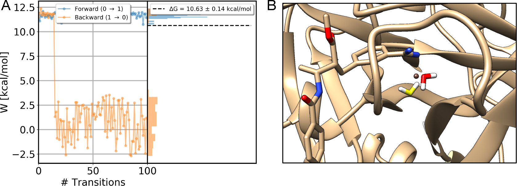
As shown in a previous study,27 one useful way to assess the quality of NES simulations is checking the overlap between non-equilibrium work distributions (Figure 5). We did this analysis for all simulated systems and we show our results from simulations of a BPTI (PDB: 5PTI) system as this system is representative about what we learned from this analysis. The NES work distributions for other systems are available at https://github.com/MobleyLab/binding_dG_water.
Figure 5:

Work values for decoupling the alchemical water in the binding site of a BPTI system (PDB: 5PTI) in forward (blue) and backward (orange) directions. The left side of each panel shows the values measured for each transition, whereas the right side shows the distribution of work values across trials. (A) and (B) are data from two replicates of NES simulations. (A) Data from simulations in the forward direction show a sudden change (circled) in work values and this transition in work values which occurs only once and is never reversed. (B) A sudden change in work values for transitions in the backward direction (circled) was also observed. Both observations suggested slow degrees of freedom in the system. The error bar is the analytical error from the BAR estimator.
In Figure 5 we found a sudden change in work values in both replicates (A,B). These changes led to a bimodal distribution of work values, indicating a slow degree of freedom of the system in simulations. Even though this did not affect our calculated free energy difference in this case (ΔG=8.25 ± 0.09 kcal/mol), it indeed reduced the overlap between the work distribution from both directions, which may bias our calculations. This potentially poor sampling of a slow degree of freedom could be more severe in simulations of other systems, so we thought it was important to trace the origin of this behavior and find solutions to improve the work distributions for robustness of this method in general cases.
We first focused on the forward direction (decoupling the alchemical water in the binding site) and found that in the EQ run the alchemical water moved from Site 1 to Site 2 in the pocket and another water molecule from bulk solvent occupied Site 1 (Figure S3). We took 100 snapshots from the EQ run as starting structures for NES simulations. We found that most of them had the alchemical water in Site 1 and a few of them close to the end of the EQ run had the alchemical water in Site 2. This explained the sudden change in work values in Figure 5A: those NES transitions which resulted in work values between 10 and 12 kcal/mol were started with a structure where the alchemical water was in Site 1 (Figure S3), whereas the other NES transitions (which resulted in work values around 2 kcal/mol) were started with a structure where the alchemical water was in Site 2 (Figure S3). For this particular binding calculation, the calculated free energy was not affected much because the majority of the transitions started from structures where the alchemical water stayed in Site 1. However, the resulting free energy could be much worse if this alchemical water moved to Site 2 or other sites earlier in simulations and did not move back quickly. Then the overlap between work distributions could be very poor and affect the final estimate from these simulations.
As discussed in Section 3, we restrained the alchemical water to the virtual site using a harmonic distance restraint to ensure that it did not move around during simulations especially when it was fully decoupled. However, in this case, the reference distance used for this harmonic restraint was 1.9 Å which is the distance between the virtual site and the alchemical water oxygen atom in the crystal structure. The restraint force constant was 2000 kcal · mol−1 · nm−2. The distance between Site 1 and 2 was around 4 Å and the virtual site was centered between Site 1 and 2 (so that both sites are around 2 Å away from the virtual site). Thus, this water motion was partially due to the non-zero (or close to zero) reference distance used in the restraint and so the alchemical water could move around while it was strongly restrained to the virtual site (e.g., while maintaining an equal restraint energy, it could sample the surface of a sphere of a radius of 1.9 Å around the virtual site (Figure S3)). This is not ideal because we applied this restraint to make sure this alchemical water stayed in the site in simulations. Instead we decided to redefine the virtual site to ensure the alchemical water stays in the same site as that revealed in the crystal structure.
We redefined the virtual site based on simulations we already performed. Ideally we aimed to define a virtual site which was very close to the alchemical water oxygen atom. To achieve that, we first calculated the root mean square fluctuation (RMSF) for all backbone and Cβ atoms. Then we selected reference atoms with a RMSF smaller than 1 Å. The reference protein atoms (atom A and atom B) and the oxygen atom of the alchemical water were selected to be nearly co-linear to ensure that the defined virtual site is close to the alchemical water oxygen atom. We calculated the angle between atom A, alchemical water oxygen and atom B and considered those that were within 5 degree of 180° for possible use as reference atoms. We checked all our six EQ runs (3 replicates × 2 end states) and found all atom A and atom B that fulfilled the requirements in terms of RMSF and angle. In the end, we used two atoms from the protein (CYS14(N) and ASN44(O)) to define a new virtual site that had a distance of 0.06 Å from the alchemical water oxygen atom.
We then performed simulations following the same protocol as the one we used for simulations with the old virtual site (Section 3). Then we confirmed that, with the new virtual site, the alchemical water stayed in the original water site (Site 1 in Figure S3) over the course of the simulation and we did not see a sudden change in work values from the forward direction.
We then focused on the sudden changes in work values for transitions in the backward direction (Figure 5B). Our analysis of trajectories from EQ runs showed that a different protein backbone conformation was favorable in simulations when the alchemical water was fully decoupled in the binding site. In Figure 6A, the oxygen atom in GLY12 preferred a inward direction in simulations (cyan) and occupied the space of the alchemical water (yellow). This orientation was very different from the crystal pose (tan). When the alchemical water was not interacting with the environment, a cavity was created because of that. The protein responded to this and changed its backbone conformation to fill this cavity.
Figure 6:

A protein backbone motion was observed in EQ simulations of a BPTI system (PDB: 5PTI) when the alchemical water was completely decoupled in the binding site. (A) A comparison between the crystal pose (tan) and simulation snapshot (cyan) showed a key structural difference in the protein backbone. The target water molecule is shown in yellow. (B) and (C) Work values for each attempted transition from two replicates and their distributions. The tan and cyan circles highlight the work values from transitions started from the two conformations shown in panel A with the same color code. The error bar is the analytical error from the BAR estimator. (D) A distance between the oxygen atom in GLY12 and the virtual site was computed to check the preferred backbone conformation during simulations. (E) and (F) The distance of the atom pair shown in panel D was computed over the course of EQ simulations. The distance change correlated well with the work values change in panel B and C.
We further monitored the distance between the oxygen atom in GLY12 and the virtual site (Figure 6D) for the 100 snapshots which were used as initial structures for NES transitions (Figure 6E–F). We found that the distance change correlated very well with the changes in work values from the 100 NES transitions (shown as orange in Figure 6B–C).
Our results suggest the bimodal distribution in Figure 6B–C was in fact due to the two different backbone conformations sampled in the equilibrium simulation which was used to seed the NES transitions (the work distributions are circled in cyan and tan in Figure 6B–C). Our nonequilibrium transition simulations were not long enough (500 ps) to allow for backbone reorganization upon water recoupling/decoupling. Extending the simulation timescale dramatically to allow for backbone rearrangement during nonequilibrium switching transitions would make this method much more expensive and lose many of the advantages in efficiency over the equilibrium methods. Alternatively, we could use a separation of states approach to keep the protein from needing to rearrange during equilibration and/or NES transitions (such as by introducing protein restraints), and then sample any requisite protein motions in a separate restraining/unrestraining step for the end states.
To improve handling of these slow rearrangements, we decided to implement position restraints on the protein atoms to prevent the binding site from collapsing (Figure 2). The alchemical water was decoupled in the binding site while the protein binding site was restrained to its original positions and the alchemical water was restrained to the virtual site.
In practice, we selected backbone atoms in residues that are within 5 Å of the alchemical water oxygen atom (Figure S4) and applied position restraints with a force constant of 239 kcal · mol−1 · nm−2. The structures were first minimized and then the selected atoms were restrained to their positions in equilibration, EQ runs and NES transition simulations. We then checked the distribution of work values from both direction transitions. As shown in Figure S5, the overlap is much improved compared to Figure 6B–C and we did not see any big jump in work values as we saw before.
To account for this position restraint on protein atoms in our calculations of ΔGbinding, we performed simulations as described in Section 3 when the alchemical water was in both the interacting and non-interacting states. We used 21 λ states in total in simulations to calculate the free energy difference between the two end states (restrained protein vs. non-restrained protein). The free energy cost of restraining the protein in the crystal pose when the alchemical water was in the interacting state was 12.2 ± 0.2 kcal/mol. The uncertainty estimate here is the standard deviation across three replicates. The free energy cost for releasing position restraints on the protein when the alchemical water was decoupled was 15.8 ± 0.1 kcal/mol. This energy cost is higher compared to the value when the alchemical water is in the interacting state because the protein backbone prefers a conformation that is different from the crystal structure when the alchemical water is decoupled (as discussed above). Therefore, the free energy cost for maintaining the protein backbone in the crystal pose is higher when the alchemical water is fully decoupled.
The calculated binding free energy of the water molecule (ΔGbinding) is −2.6 ± 0.3 kcal/mol from simulations with the protein restraints and −1.9 ± 0.4 kcal/mol from simulations where the protein was not restrained. The difference in numerical values was not that substantial in this case. Still, this allowed us to avoid a clear sampling problem, and the approach ought to generalize to cases where protein motion causes larger errors.
Originally we used 21 λ states in simulations to correct for the position restraints used on protein atoms, but we wanted to determine whether we could use a subset of these intermediate states to save computational time while still retaining the accuracy of our calculations. To test this, we reduced the number of intermediate λ states and we wanted to find an automated procedure to select a reasonable λ schedule for a given number of intermediate states.
We first created all possible combinations of our fixed set of of λ values with a given number of total states (in this case, 2 to 21). For each combination, we ensured the two end states were included (λ=0, 1). Then we calculated the corresponding overlap matrix for each combination and checked tridiagonal elements off of the diagonal (the diagonals above and below the main diagonal). If any of these tridiagonal values ((Oi,j,(i≠j))) was below 0.03 (as suggested by previous work1), this combination of λ values was discarded. We did this filtering operation for each simulation trial (3 in total). Then we ranked each remaining combination of λ states with the average and standard deviation of tridiagonal values over the three simulation trials. We picked the best combination (λ schedule) with a given number of states that maximized the average tridiagonal values and minimized the standard deviations of tridiagonal values over three simulation trials.
With only two λ states (λ=0, 1), the overlap between state 0 and 21 was 0. With three states (any λ state plus λ = 0, 21 ), no λ schedule fulfilled our requirements described above for filtering. Only with 4 λ states, we found reasonable overlap between these states. Here, we considered a overlap over 0.1 as sufficient. As shown in Figure S6A–C, for simulations correcting the position restraints on protein atoms when the alchemical water was in the interacting state, 4 λ states are enough to achieve sufficient overlap. When releasing position restraints when the alchemical water was decoupled, 5 λ states were necessary to achieve good overlap between states. This was a substantial reduction from the 21 states we started with.
With 4 λ states, the overlap between λ = 0.95 and λ = 1.0 was lower than our preferred value, 0.1, but still larger than the cutoff of 0.03. The lowest level of overlap was between those two states, but could not be improved further given our predefined set of lambda values. We checked other tridiagonal values when we determined how many λ states were necessary to achieve a sufficient overlap with a cutoff of 0.1 as we mentioned above. It is likely the case that the overlap could be improved further (or the number of λ values further reduced) with additional tuning of the number and spacing of λ states in future work.
These results indicate that not all 21 λ states are necessary for converged results for these restraint correction simulations. Only a few of them are actually needed to achieve good overlap bridging the two end states. More λ states near the unrestrained end state (lambda = 1.0 in this case) are needed to ensure good overlap (Figure S6) since λ = 0.95 is always selected in our final λ schedule (Figure S6).
4.1.3. Protein and ligand motions affected the work distribution in simulations of other systems.
In simulations of a scytalone dehydratase system (PDB: 3STD), we observed contrary trends in work values from the forward direction in two replicates (Figure 7A–B). We found that a ligand motion contributed to this difference in work values. When the proton on the nitrogen atom (circled in Figure 7C–D) was close to the alchemical water (red blob in Figure 7C and D), the work values from the forward direction increased (~ 10–12 kcal/mol). In contrast, when the proton pointed away from the alchemical water (tan and cyan structures in Figure 7C and D, respectively), the work values got much lower (~ 4–6 kcal/mol). The difference in work values due to this ligand motion was about 6 kcal/mol.
Figure 7:

In EQ simulations of a scytalone dehydratase system (PDB: 3STD) we observed a ligand motion that potentially affected hydrogen bond formation between the proton on the nitrogen atom of the ligand and the alchemical water. In NES simulations in the forward direction, the work distribution was affected depending on the distance between the distance between the proton on the nitrogen atom of the ligand and the alchemical water. (A) and (B) Work values for each attempted transition from two replicates and their distributions. The error bar is the analytical error from the BAR estimator. (C) and (D) Snapshots extracted from simulations (first and last frame) of the two replicates shown in (A) and (B) highlight the ligand motion (red circle).
The protein motion also contributed to the difference in work values of the backward direction (Figure 7A–B). In Figure 7A and B, the work distribution in the backward direction has a peak between 6–8 kcal/mol and between 2–4 kcal/mol, respectively. We found a histidine side chain orientation differed in EQ runs for these two replicates. The histidine maintained the crystal pose and the ring was oriented edge-on towards the alchemical water in simulations that returned work values shown in Figure 7A. But in other replicates the histidine ring pointed away from the alchemical water (Figure S7). Since this histidine was known to form a hydrogen bond with the target water molecule in the crystal structure,17 its side chain orientation might substantially affect the work values from the backward direction transitions.
4.1.4. The work distribution can be affected by unwanted water rehydration in the binding pocket when the alchemical water is fully decoupled in EQ runs.
When the alchemical water is decoupled in the binding site, we observed that water molecules from bulk solvent refilled this ”empty” site in EQ runs of a FXa system, leading to a sudden change in NES work distributions (Figure 2). This unexpected rehydration results in two water molecules occupying the binding site in very close proximity: the decoupled alchemical water (water A) and an extra water from bulk solvent (water B). When we recouple the alchemical water in NES transitions, water A interacts with water B initially. The final work value is not just for recoupling water A but also includes the energy cost associated with the interaction with water B. If water B gets trapped in the site then we may end up with two water molecules in the binding site until the end of NES transitions. This results in a different number of water molecules in the binding site in the two end states for transitions when recoupling the water relative to transitions when decoupling the water. So the overlap in work distributions between the two directions can be very poor. Additionally, as we discussed in Section 4.1.1, the goal is to calculate the free energy for decoupling/recoupling this single alchemical water so if the computed free energy also include the contribution of interacting with other unexpected water molecules in the binding site, then the calculation includes states which are outside of the integration region.
Figure 8 shows an example from simulations of a FXa system (PDB: 1EZQ), where we see a sudden change in work values from transitions in the backward direction (orange in Figure 8A). We found in EQ runs a water molecule from bulk solvent refilled the site where the decoupled alchemical water was located (Figure 8B). So in transition simulations in Figure 8A (orange), the 100 starting structures came from two different metastable states that differed in whether the extra water was present or not. The work values were significantly different depending on the number of water molecules in the binding site in these starting structures.
Figure 8:
Water molecule entry led to sudden changes in work values when water entered the binding site during EQ runs of a FXa system (PDB: 1EZQ) when the alchemical water was fully decoupled. (A) The work distributions mostly do not overlap, and this was caused by an alchemical water moving into the binding site when the alchemical water was decoupled in the binding site during an EQ run (shown in B). The error bar is the analytical error from the BAR estimator. (B) A snapshot of the non-interacting alchemical water in the binding site, drawn from an EQ run. The alchemical water is shown in yellow and the water from bulk solvent is shown in red. The brown blob is the virtual site.
We also observed similar water motion in a scytalone dehydratase system (PDB: 3STD). We have discussed how protein/ligand motions affected the work distribution in Figure 7. In one replicate simulation, a water molecule from bulk solvent moved into the hydration site during EQ runs (Figure S8B). So the starting points extracted from this segment of the EQ simulation (red circle in Figure S8A) had a different number of water molecules in the binding site compared to other starting points. This also affected the overlap between work distributions and thus impaired the accuracy of the estimated free energy difference between the two end states.
One could prevent the problem of poor overlap between work distributions due to trapped water by applying a potential to repulse water molecules from bulk solvent so they cannot move closer to the binding site. One example could be a hard-wall potential. However, this seems not to be available in GROMACS yet so it has not been tested in the present work.
Alternatively, as described in Section 4.1.1, we can carefully define our integration region55 by selecting for analysis a subset of our data in which only the alchemical water was in the binding site. We tested this idea in the FXa system where a water from bulk solvent entered the binding site when the alchemical water was completely decoupled (Figure 8). We discarded simulation data for transitions which started from a structure that had extra water molecule in the binding site. Using this approach, we discarded 85% of the simulation data from this replicate. But this data was outside of the integration region since no water molecules (other than the decoupled alchemical water) should be in the binding site in simulations of this end state, and thus this data impaired convergence. After discarding this data, the overall calculated ΔG (11.71 ± 0.01 kcal/mol, uncertainty estimated as the standard deviation of results from three simulation replicates) from these simulations has a lower standard deviation across the three replicates than the original calculations (11.35 ± 0.51 kcal/mol) suggesting better convergence of the calculation (Figure S9).
While this procedure did result in a dramatic loss of available data for this particular replicate, the calculated ΔG value after discarding this data ended up very close to the other two replicates which did not have problematic data, further validate this approach of carefully defining the integration region.
4.1.5. Unexpected behavior of the alchemical water when electrostatics and sterics were switched simultaneously in NES transitions.
Initially, we simultaneously turned on/off both vdW and Coulomb interactions of the alchemical water during NES simulations. However, we found that the work values from some transitions were significantly lower (anomalously negative) than other work values in NES simulations recoupling the alchemical water (Figure S10A–C). Our analysis revealed that one chloride ion moved very close to the alchemical water oxygen atom during NES transitions which involved turning on the interactions of the alchemical water in the bulk solvent (Figure S11). Transitions where we observed this issue all returned anomalously negative work values as shown in Figure S10A–C which made our final estimated free energy difference incorrect.
We do not fully understand the origin of this chloride ion motion, but it seems to be an artifact of the chosen thermodynamic path, as we were able to find a way to work around the problem via an alternate path. As described in Section 3, we switched to turning on/off vdW and Coulomb interactions of the alchemical water separately in NES simulations. When we did so, no chloride ions moved close to the alchemical water oxygen atom in our simulations and a good overlap between work distributions was obtained in each replicate (Figure S10D–F). The calculated solvation free energy of the alchemical water (TIP4P water model) is −6.13 ± 0.01 kcal/mol which agreed well with the computed value in a previous study56 (−6.11 kcal/mol) and the experimental data (−6.33 and −6.32 kcal/mol in ref57,58).
4.1.6. The protocol can be optimized for higher efficiency.
The simulation protocol used in this work was adopted from a previous study of ligand binding free energy calculations27 and we were interested in optimizing the protocol for higher efficiency for water simulations. While more future work is needed for this goal, here we present our results of preliminary tests to show the potential of further efficiency optimization.
We picked 3 systems (FXa, PDB: 1LPG; scytalone dehydratase, PDB: 4STD; HIV-1 protease, PDB: 1EC0) where NES simulations of decoupling the alchemical water in the binding site returned converged results with the original protocol (EQ run: 20 ns, NES transitions: 500 ps). Note that in these tests, we did not implement position restraints on protein atoms but only restrained the alchemical water to the virtual site.
We first reduced timescales of NES transition simulations from 500 ps to 250, 125, 50 and 5 ps while keeping other simulation details the same as the original protocol (see Section 3). The results are shown in Figure 9A–C. Reducing the transition time by 99% from the original timescale (500 ps) did not affect the calculated ΔG much. As we changed the timescale from 500 ps to 5 ps, the calculated ΔG only changed 1.5%, 8.5%, 4.3% (|ΔG500ps − ΔG5ps|/ΔG500ps) for FXa, scytalone dehydratase and HIV-1 protease, respectively. The absolute value of differences between results from 500 ps and 5 ps simulations were smaller than 0.5 kcal/mol in all tested systems. The error bars were larger in results from 5 ps simulations compared to 500 ps simulations but were still less than 1 kcal/mol.
Figure 9:
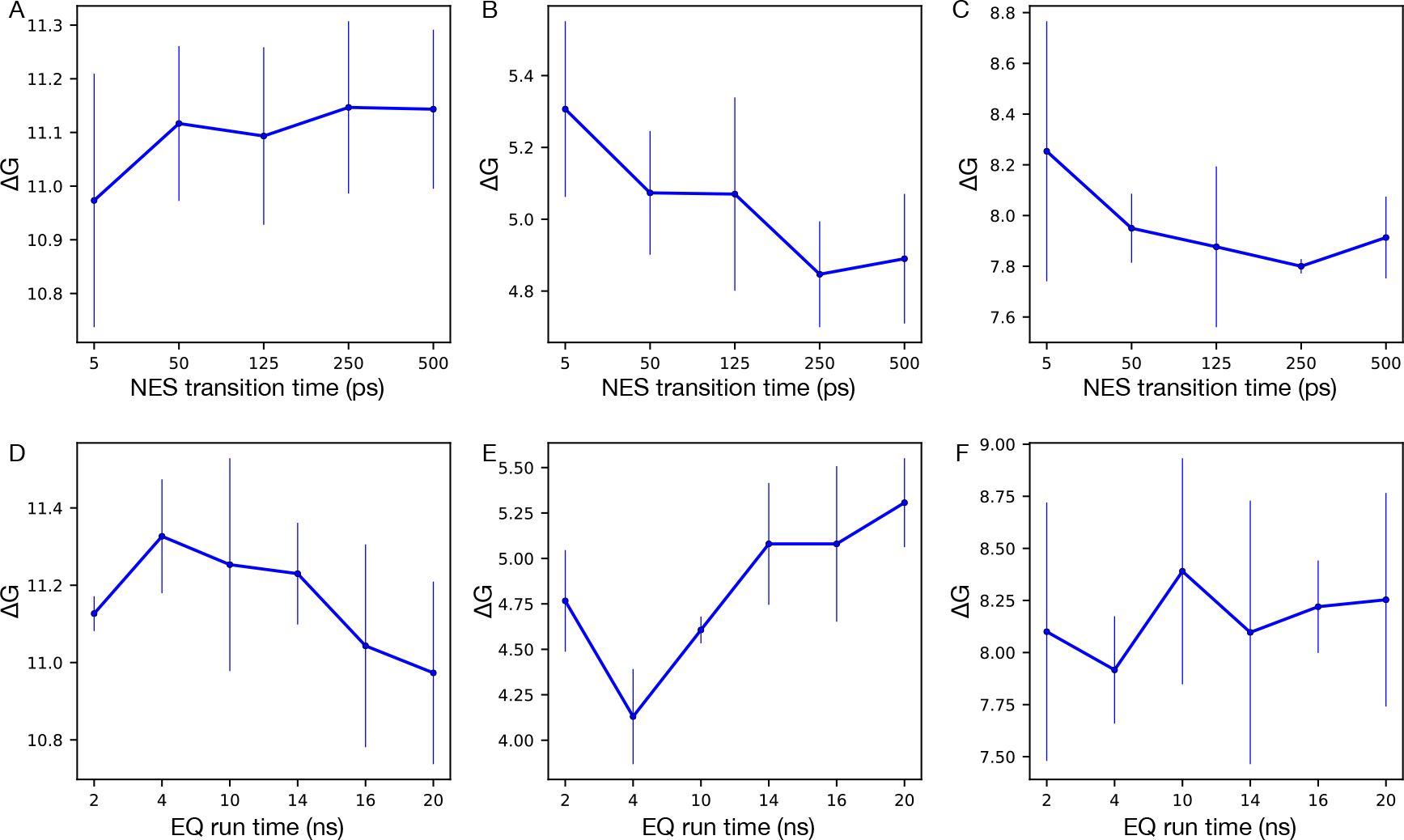
Calculated free energy differences between the two end states in NES simulations of decoupling the alchemical water in the binding site using different NES transition timescales (A-C) and different EQ run timescales (D-F). Three systems were selected for this test: A,D: FXa (PDB: 1LPG), B,E: scytalone dehydratase (PDB: 4STD), C,F: HIV-1 protease (PDB: 1EC0). We showed averaged and standard deviation values from three replicates for each system.
We then tested reducing the timescale of EQ runs used to sample the end states. The starting structures of NES simulations were collected from these EQ runs. We used 6 different timescales in our tests: 2, 4, 10, 14, 16, and 20 ns (20 ns was the original set-up, see Section 3). Based on our results from NES timescale test simulations (see above), we used 5 ps as the NES transition timescale in these tests. All other simulation set-up was the same as the original protocol (Section 3).
As shown in Figure 9D–F, the change in calculated ΔG between simulations using 2 ns of equilibration versus those with 20 ns was small (1.4% for FXa, 1.9% for HIV-1 protease). The ΔG difference between simulations with 2 ns and 20 ns was slightly larger than 10% for scytalone dehydratase (10.2%). Similarly, the error bar in HIV-1 protease results (Figure 9F) was larger than 1 kcal/mol when 2 ns was used for EQ runs, suggesting that longer simulations were needed for improved convergence.
These results were promising since they suggested a much shorter timescale could be used in EQ runs and NES simulations while still retaining similar accuracy in calculations, at least for systems where this protocol is well-behaved. However, this optimization was tested only on these three cases. In other systems studied above (Section 4.1.1, 4.1.2, 4.1.3, 4.1.4), we found sampling challenges in our simulations and even our original protocol with longer timescale was not sufficient for converged estimates of the free energy difference (Figure 2). Thus, a key avenue for further inquiry is to determine whether well-behaved versus slow systems can be anticipated/identified in advance; if so, a dramatically more efficient protocol could be used for well-behaved systems while slow/difficult systems could be reserved for treatment with alternate methods.
4.2. Discrepancies are observed between our calculated binding free energies and the literature values.
As we mentioned above, these 13 systems had been previously studied.17 But reproducing those literature values is not the top goal in this work, because the prior values have not been verified by comparison to experimental data nor have they been independently verified in another study, to our knowledge. Thus, it is difficult to be certain that the prior calculations truly provide gold standard values. Ideally, we are interested in comparing our calculated values with the underlying experimental reality. However, experimentally determined binding free energies of water molecules are generally not available due to the difficulty of defining and measuring such values. Thus, we compared our results with the literature values17 (Figure 10), though these do not necessarily provide a gold standard.
The prior calculations also used a somewhat different definition of the thermodynamic state being considered, making our results not strictly comparable. In particular, the prior study used a different set of restraints. In the previous work,17 the alchemical water was restrained to the site with a hard-wall potential in which no bias was applied when the target water was in a region defined with a radius whereas infinite repulsive barriers were applied beyond the radius. This hard-wall potential ensured the target water stayed in the binding site and no other particles (e.g., protein, ligand or other waters) could enter the region. In our work, we used a single harmonic distance restraint on the alchemical water and the defined virtual site (see Section 3) which did not prevent bulk water molecules and/or the protein or ligand from occupying the position that is vacated by the fully decoupled alchemical water. Because of the different choice of applied restraints, the results from this previous study represent the free energy of the alchemical water binding to a pre-formed cavity. This is different in an important way from the present study; here, our calculated ΔGbinding reflects the free energy of the alchemical water binding as well as cavity formation (when it is necessary), such as for cavities created by protein or ligand rearrangements needed to make room for the water.
Overall, no correlation is observed between our results and the literature values (Figure 10) even though our results on BPTI and Factor Xa agree better with the literature values (RMSE of 0.1 kcal/mol for BPTI and R2 of 0.9 for Factor Xa) than those on other protein targets (HIV-1 protease, trypsin and scytalone dehydratase) (Table S1). Due to factors we mentioned above, we are not surprised by discrepancies between our results and the literature values. We further discuss possible reasons for the discrepancies between our results and literature values in Section 5.
5. DISCUSSION
In this work we are interested in developing a NES based method for efficient and accurate binding free energy calculations for water molecules. Long-term, we are potentially interested in using a separation of states approach to treat slow water insertion/deletion events separately from ligand transformations in relative binding free energy calculations. To do so, we would need an efficient method for computing the contributions of water insertion/deletion to binding, or what one might call water binding free energy calculations.
Here, we have not explored whether NES approaches are more efficient than equilibrium approaches for water binding free energy calculations, but the NES approach has several advantages over equilibrium approaches for the specific case of buried water molecules. The most important advantage of the NES approach is that the system may be out of equilibrium as it passes through the intermediate states, which is particularly important for the water molecules being inserted or displaced. In contrast, with an equilibrium approach (for ligand binding or water insertion/deletion) the system must be at equilibrium at each intermediate state. For water insertion/deletion, equilibrium intermediate states can in some cases be hard to define or describe – e.g. if one water is being removed and is only very weakly interacting, perhaps all other water molecules in the box ought to swap in and out of the same position at equilibrium, making sampling very difficult. Of course, such exchanges do not necessarily have to impede convergence, depending on how the calculation is set up,59 but practical considerations mean it will be difficult to know whether the calculation is converged of no exchanges take place. Additionally, especially in states where the alchemical water is (partially) decoupled, such slow exchanges may result in other water molecules becoming trapped in and competing for space in the binding site. Nonequilibrium techniques potentially allow a single water to be inserted or deleted into a site relatively rapidly without having to compete with other (chemically equivalent) waters for the space, simplifying this issue. While nonequilibrium calculations do not completely avoid the complexities which might arise with equilibrium calculations, transitions in which alternate waters attempt to enter the binding site can be filtered out to ensure the relevant separation of states remains valid.
The NES approach also has other advantages over equilibrium approaches. First, the NES approach can potentially be used with very short switching timescales (e.g., ps) whereas equilibrium approaches typically require fairly long timescales (e.g., ns). Second, in the NES approach a large number of transition simulations between the two end states are performed to obtain converged estimates, making this approach highly parallelizable and ideal for distributed computing environments when they are available. This can significantly reduce the wall-clock time for these calculations.
Given these advantages of the NES approach, we explored using it for accurate and efficient calculation of binding free energy of water molecules in this work. To our best knowledge, this is the first time that the NES approach has been used for calculating ABFE of water molecules. So we analyzed our simulations and identified issues that affected the accuracy and convergence of our calculation. We hope the lessons we learned are helpful for future method development and research in this area.
In restraint correction simulations for multiple systems we observed that the alchemical water escaped from the binding site when it was not restrained (Section 4.1.1). We addressed this problem by carefully defining the region of integration55 and excluding simulation data where the alchemical water was not in the bound state. When we used this approach to compute the free energy cost of applying or releasing the harmonic distance restraint on the alchemical water, we found that the free energy estimate converged much faster.
We found the BAR estimator still yielded precise free energy estimates here, even after excluding data where the alchemical water unbound. But in the case when the remaining data after discarding is not enough for converged estimate of the free energy cost, running more replicate simulations or including more intermediate states in simulations may serve better. Moreover, since the bound state definition is artificial, it is important to carefully examine the dependence of the results on this definition for studied systems for any future work (i.e., we tested different distance cutoffs in this work).
We observe water unbinding in only some restraint correction simulations, suggesting this phenomenon is highly system dependent. In this work, we observed it more frequently in HIV-1 protease and scytalone dehydratase simulations than other systems we studied. In one scytalone dehydratase simulation (PDB: 4STD), this issue led to abnormally large error bars (Figure 10A). In other systems, we only observed at most one replicate that had water unbinding in simulations when the alchemical water was not restrained.
In addition to water-specific considerations noted above, our analysis in this work is subject to the standard constraints on overlap which affect NES-based approaches in general. Previous work showed that the NES approach had limitations especially in achieving convergence. The work distributions of two directions should overlap sufficiently so that an accurate estimate of the free energy change can be obtained. Otherwise, the results calculated based on equation 1 becomes the mean of forward and backward exponential averages computed using the Jarzynski equality. It is known that the tails of the distribution dramatically affect the results of exponential averaging60 and the samples are normally rare in these tails. So when the overlap between the bidirectional work distribution is poor, the estimated free energy difference from NES simulations become unreliable.
In this work, we explored reasons for the sudden change in NES work distributions (Section 4.1.2, 4.1.4, 4.1.3). In fact, many of these reasons stem from sampling during the EQ runs prior to NES simulations, as starting structures for NES transitions were collected from these EQ runs. So if there was a slow motion that was not well sampled during EQ runs, then the collected structures from these runs for NES transitions have different protein/ligand conformations and/or with different numbers of water in the binding site (Section 4.1.2, 4.1.4, 4.1.3). The work values of NES transitions are affected by these starting structures and the resulted work distributions may overlap poorly, especially if the sampling EQ runs were inadequate.
For example, one challenge we noticed in EQ simulations of the BPTI system (PDB: 5PTI) is the protein binding site collapsed when the alchemical water was fully decoupled in the binding site. While the collapse did not affect our calculations much, it could be a major problem in such calculations for other systems since the protein conformation exhibited substantial differences between the two end state EQ simulations. So the overlap between NES work distributions could be very poor if the simulation time was not enough to sample both conformations during NES transitions.
Slow protein motions could be well sampled by increasing transition times, but we do not recommend this approach because the time required for backbone conformational change (e.g., moving between an open versus closed binding site) could be very slow and is normally not known in advance. So the computational cost of this approach can be very high. Because of these considerations, in this work we applied position restraints on protein atoms to prevent the binding site from collapsing when the alchemical water was decoupled in the binding site. Our results for the BPTI system show that restraining the protein binding site atoms indeed avoided sampling the slow protein backbone motion in the presence/absence of the alchemical water and a correct estimate of the free energy cost was obtained. However, this approach does require more simulations for these additional edges, increasing the computational cost. However, with these additional simulations the binding free energy estimates of the alchemical water (ΔGbinding) converged faster without the need of sampling the slow protein backbone motions. Compared to our original workflow, we find that the use of binding site restraints provides a more robust approach for use in prospective studies where it is not clear whether the protein binding site will collapse or not when the alchemical water is decoupled. Meanwhile, the computational cost of running simulations with these position restraints is not necessarily high. In fact, as we showed in this work only 4 λ states including the two end states are needed for correcting such restraints in our final estimated ΔGbinding. Meanwhile, since the protein is restrained in EQ runs, the timescale for EQ runs can be shortened to further lower the overall computational cost.
These sampling issues (e.g., water unbinding, protein/ligand motions) were also observed in some NES transitions for some systems. But they did not affect our calculations of ΔG for these edges. We performed 3 replicates with 100 NES transitions for each direction in each replicate as described in Section 3. So even in the worst case, we always had at least 200 transitions after discarding data due to these protein/ligand/water motions (Section 4.1.2, 4.1.4, 4.1.3) which is still enough to estimate ΔG for the two end states.
Besides identifying sampling issues, we also did some preliminary optimization of our protocol’s efficiency. The simulation protocol was adapted from a protocol which was designed for absolute binding free energy calculations for small molecules.27 Our results suggest that the computational cost of our method can be reduced for most systems in this work and there is still space to optimize it in the future work.
A poor agreement is observed between our results and the literature values17 especially for HIV-1 protease and scytalone dehydratase systems (Table S1. The first potential origin of the discrepancies is force field. But as we mentioned in the Methods section (Section 3), we used the same protein force field and water model as the previous study. The small molecule force field used in this work (OpenFF) was different from the previous study (GAFF) but we expect these two force fields to yield similar binding free energies.61 So the discrepancies are likely not caused by the selected force field.
We identified sampling problems that affected the convergence of our calculations. For example, we performed simulations to account for releasing the harmonic distance restraint between the alchemical water and the virtual site. The results from these simulations especially for scytalone dehydratase systems were very noisy due to the poor phase space overlap between the two end states (Section 4.1.1). But even when we re-analyzed our data using just bound state snapshots (see Section 4.1.1), the calculated overall ΔGbinding values were still not close to the literature values.
We next checked our NES simulations and found the overlap between work distributions was poor in simulations of one HIV-1 protease system (PDB: 1HPX) due to protein motions when the alchemical water was fully decoupled. However, in other HIV-1 protease systems where we observed sufficient overlap between work distributions and obtained converged results (error bar smaller than 0.6 kcal/mol between three replicates), the calculated ΔGbinding was still not close to the literature value. We had similar observations in simulations of scytalone dehydratase.
The reference values we used in this work are the calculated ΔGbinding for these systems from a previous study17 (Barillari et al., 2007). These reference values did not agree with the results from other previous studies on one HIV-1 protease system (PDB: 1HPX).62,63 The authors of the previous study17 ((Barillari et al., 2007)) also noticed the discrepancy in this HIV-1 protease system. They suggested that the difference was due to the different restraints used for fully decoupled water in the binding site. In their work, they used a hard-wall potential to restrain the water in the binding site. This restraint also prevented unwanted water molecules and protein/ligand atoms from occupying the position that is vacant by the fully decoupled alchemical water. However, other previous studies62,63 (Hamelberg et al., 2004; Lu et al., 2006) on this system used a harmonic potential to restrain just the alchemical water in its position in the binding site. This harmonic potential restraint was similar to the restraint we used in our work. In fact, our calculated ΔGbinding for this HIV-1 system agrees with these literature values where a similar harmonic potential restraint was used on the alchemical water.
Our calculated ΔGbinding reflects the free energy cost of water binding and cavity formation whereas in the previous work using the hard-wall potential, the calculated ΔGbinding only reflects the binding free energy of a water molecule in a pre-existing cavity, as noted above. Thus, for systems where the binding site collapses when the alchemical water is fully decoupled, we should expect different results from our simulations compared to the literature values because of this important difference in the property being calculated. Our observations back this up; we indeed found more protein/ligand motions that affected our calculations in the HIV-1 protease and scytalone dehydratase simulations, and these were the systems where our results deviated most significantly from the literature value.
Another reason that may also explain the discrepancies between our results and the literature values is the input structure of simulations. We tried to be consistent with the previous study (Barillari et al., 2007).17 For the input structures, we started our preparation using the same PDB code. For protonation states of binding site residues that were described in their paper, we prepared our input structures with the same protonation states. But still, since the prior study did not provide the actual input structures used in the simulations, we may have differences in protonation states for other residues which might lead to differences in our calculated results when comparing to the literature values.
It is not necessarily clear that correct water binding calculations should reproduce the results of prior work; after all, results from these prior studies could also have been affected by some of the same sampling issues as identified in this work, and we lack the ability to check the prior work for sampling and convergence problems. Additionally, experimental binding free energies are typically not available, including for these studied water sites and the best we can do in this work is to compare our results with available calculated numbers from the literature. Given sampling challenges identified in this work, such comparisons may be challenging.
In future, we hope to test our proposed ”separation of states” idea on protein-ligand systems where water rearrangement poses sampling issues in RBFE calculations or the displacement of a buried water affect the measured binding potency of two ligands. We hope to use available experimental measured binding free energy difference between ligands (ΔΔG) to assess the effectiveness of our method for endpoint corrections.
6. CONCLUSION
In this work, we developed a non-equilibrium switching based approach to calculate binding free energies of waters in selected sites in a binding pocket. We identified sampling problems that affected our calculations and provided ways to help address them. For example, using position restraints on protein atoms can prevent our calculations from being affected by a binding site collapse in simulations when water sites are emptied. Additionally, we can carefully define the integration region (the ”bound state”) and only use relevant data in analysis, improving convergence. The lessons that we have learned from this work will be very helpful for future work on handling water sampling for RBFE calculations via separation of states.
Supplementary Material
7. ACKNOWLEDGEMENTS
We appreciate financial support from the National Institutes of Health (1R01GM108889-01 and 1R01GM124270-01A1) and from XtalPi and Pfizer, as well as computing support from the UCI Research Cyberinfrastructure Center, supported in part by NSF Grant CNS-1828779. The content is solely the responsibility of the authors and does not necessarily represent the official views of the National Institutes of Health. We thank Mary Pitman and Trevor Gokey for their help in evaluating the restraint correction term used in our calculations.
Footnotes
D.L.M. is a member of the Scientific Advisory Board of OpenEye Scientific Software and an Open Science Fellow with Roivant.
ASSOCIATED CONTENT
Supporting Information Available
Supporting information is available free of charge via the Internet at http://pubs.acs.org.
Supporting figures of water/protein motions in simulations, calculated ΔG with different amount of input data, selected atoms used for backbone restraints, work distribution from NES simulations of different systems and how water motions affect the distribution, phase space overlap matrix, a simulation snapshot showing a chloride ion approaching to the alchemical water; a table summarizing all calculated ΔG, literature values and statistics.
Additional Information Available: Input files for simulations and NES work distributions are freely available at: https://github.com/MobleyLab/binding_dG_water.
References
- (1).Mey AS; Allen BK; Bruce Macdonald HE; Chodera JD; Hahn DF; Kuhn M; Michel J; Mobley DL; Naden LN; Prasad S; Rizzi A; Scheen J; Shirts MR; Tresadern G; Xu H Best Practices for Alchemical Free Energy Calculations [Article v1.0]. LiveCoMS 2020, 2, 18378. [DOI] [PMC free article] [PubMed] [Google Scholar]
- (2).Bortolato A; Tehan BG; Bodnarchuk MS; Essex JW; Mason JS Water Network Perturbation in Ligand Binding: Adenosine A 2A Antagonists as a Case Study. J. Chem. Inf. Model. 2013, 53, 1700–1713. [DOI] [PubMed] [Google Scholar]
- (3).Zia SR; Gaspari R; Decherchi S; Rocchia W Probing Hydration Patterns in Class-A GPCRs via Biased MD: The A 2A Receptor. J. Chem. Theory Comput. 2016, 12, 6049–6061. [DOI] [PubMed] [Google Scholar]
- (4).Huang D; Rossini E; Steiner S; Caflisch A Structured Water Molecules in the Binding Site of Bromodomains Can Be Displaced by Cosolvent. ChemMedChem 2014, 9, 573–579. [DOI] [PubMed] [Google Scholar]
- (5).Crawford TD; Tsui V; Flynn EM; Wang S; Taylor AM; Côté A; Audia JE; Beresini MH; Burdick DJ; Cummings R; Dakin LA; Duplessis M; Good AC; Hewitt MC; Huang H-R; Jayaram H; Kiefer JR; Jiang Y; Murray J; Nasveschuk CG; Pardo E; Poy F; Romero FA; Tang Y; Wang J; Xu Z; Zawadzke LE; Zhu X; Albrecht BK; Magnuson SR; Bellon S; Cochran AG Diving into the Water: Inducible Binding Conformations for BRD4, TAF1(2), BRD9, and CECR2 Bromodomains. J. Med. Chem. 2016, 59, 5391–5402. [DOI] [PubMed] [Google Scholar]
- (6).Woodhead AJ; Angove H; Carr MG; Chessari G; Congreve M; Coyle JE; Cosme J; Graham B; Day PJ; Downham R; Fazal L; Feltell R; Figueroa E; Frederickson M; Lewis J; McMenamin R; Murray CW; O’Brien MA; Parra L; Patel S; Phillips T; Rees DC; Rich S; Smith D-M; Trewartha G; Vinkovic M; Williams B; Woolford AJ-A Discovery of (2,4-Dihydroxy-5-Isopropylphenyl)-[5-(4-Methylpiperazin-1-Ylmethyl)-1,3-Dihydroisoindol-2-Yl]Methanone (AT13387), a Novel Inhibitor of the Molecular Chaperone Hsp90 by Fragment Based Drug Design. J. Med. Chem. 2010, 53, 5956–5969. [DOI] [PubMed] [Google Scholar]
- (7).Kung P-P; Sinnema P-J; Richardson P; Hickey MJ; Gajiwala KS; Wang F; Huang B; McClellan G; Wang J; Maegley K; Bergqvist S; Mehta PP; Kania R Design Strategies to Target Crystallographic Waters Applied to the Hsp90 Molecular Chaperone. Bioorg. Med. Chem. Lett. 2011, 21, 3557–3562. [DOI] [PubMed] [Google Scholar]
- (8).Smith CR; Dougan DR; Komandla M; Kanouni T; Knight B; Lawson JD; Sabat M; Taylor ER; Vu P; Wyrick C Fragment-Based Discovery of a Small Molecule Inhibitor of Bruton’s Tyrosine Kinase. J. Med. Chem. 2015, 58, 5437–5444. [DOI] [PubMed] [Google Scholar]
- (9).Ramsey S; Nguyen C; Salomon-Ferrer R; Walker RC; Gilson MK; Kurtzman T Solvation Thermodynamic Mapping of Molecular Surfaces in AmberTools: GIST. J. Comput. Chem. 2016, 37, 2029–2037. [DOI] [PMC free article] [PubMed] [Google Scholar]
- (10).Beglov D; Roux B An Integral Equation To Describe the Solvation of Polar Molecules in Liquid Water. J. Phys. Chem. B 1997, 101, 7821–7826. [Google Scholar]
- (11).Grant JA; Pickup BT; Nicholls A A Smooth Permittivity Function for Poisson-Boltzmann Solvation Methods. J. Comput. Chem. 2001, 22, 608–640. [Google Scholar]
- (12).Michel J; Tirado-Rives J; Jorgensen WL Prediction of the Water Content in Protein Binding Sites. J. Phys. Chem. B 2009, 113, 13337–13346. [DOI] [PMC free article] [PubMed] [Google Scholar]
- (13).Abel R; Young T; Farid R; Berne BJ; Friesner RA Role of the Active-Site Solvent in the Thermodynamics of Factor Xa Ligand Binding. J. Am. Chem. Soc. 2008, 130, 2817–2831. [DOI] [PMC free article] [PubMed] [Google Scholar]
- (14).Young T; Abel R; Kim B; Berne BJ; Friesner RA Motifs for Molecular Recognition Exploiting Hydrophobic Enclosure in Protein–Ligand Binding. Proc. Natl. Acad. Sci. U.S.A 2007, 104, 808–813. [DOI] [PMC free article] [PubMed] [Google Scholar]
- (15).Woods CJ; Malaisree M; Hannongbua S; Mulholland AJ A Water-Swap Reaction Coordinate for the Calculation of Absolute Protein–Ligand Binding Free Energies. J. Chem. Phys. 2011, 134, 054114. [DOI] [PubMed] [Google Scholar]
- (16).Hamelberg D; McCammon JA Standard Free Energy of Releasing a Localized Water Molecule from the Binding Pockets of Proteins: Double-Decoupling Method. J. Am. Chem. Soc. 2004, 126, 7683–7689. [DOI] [PubMed] [Google Scholar]
- (17).Barillari C; Taylor J; Viner R; Essex JW Classification of Water Molecules in Protein Binding Sites. J. Am. Chem. Soc. 2007, 129, 2577–2587. [DOI] [PubMed] [Google Scholar]
- (18).Ben-Shalom IY; Lin Z; Radak BK; Lin C; Sherman W; Gilson MK Accounting for the Central Role of Interfacial Water in Protein–Ligand Binding Free Energy Calculations. J. Chem. Theory Comput. 2020, 16, 7883–7894. [DOI] [PMC free article] [PubMed] [Google Scholar]
- (19).Ross GA; Russell E; Deng Y; Lu C; Harder ED; Abel R; Wang L Enhancing Water Sampling in Free Energy Calculations with Grand Canonical Monte Carlo. J. Chem. Theory Comput. 2020, 16, 6061–6076. [DOI] [PubMed] [Google Scholar]
- (20).Bergazin TD; Ben-Shalom IY; Lim NM; Gill SC; Gilson MK; Mobley DL Enhancing Water Sampling of Buried Binding Sites Using Nonequilibrium Candidate Monte Carlo. J Comput Aided Mol Des 2021, 35, 167–177. [DOI] [PMC free article] [PubMed] [Google Scholar]
- (21).Melling O; Samways M; Ge Y; Mobley D; Essex J Enhanced Grand Canonical Sampling of Occluded Water Sites Using Nonequilibrium Candidate Monte Carlo. ChemRxiv 2022, [DOI] [PMC free article] [PubMed] [Google Scholar]
- (22).Bodnarchuk MS Water, Water, Everywhere. . . It’s Time to Stop and Think. Drug Discovery Today 2016, 21, 1139–1146. [DOI] [PubMed] [Google Scholar]
- (23).Samways ML; Taylor RD; Bruce Macdonald HE; Essex JW Water Molecules at Protein–Drug Interfaces: Computational Prediction and Analysis Methods. Chem. Soc. Rev. 2021, 50, 9104–9120. [DOI] [PubMed] [Google Scholar]
- (24).Ge Y; Wych DC; Samways ML; Wall ME; Essex JW; Mobley DL Enhancing Sampling of Water Rehydration on Ligand Binding: A Comparison of Techniques. J. Chem. Theory Comput. 2022, 18, 1359–1381. [DOI] [PMC free article] [PubMed] [Google Scholar]
- (25).Mobley DL; Klimovich PV Perspective: Alchemical Free Energy Calculations for Drug Discovery. The Journal of Chemical Physics 2012, 137, 230901. [DOI] [PMC free article] [PubMed] [Google Scholar]
- (26).Gapsys V; Yildirim A; Aldeghi M; Khalak Y; van der Spoel D; de Groot BL Accurate Absolute Free Energies for Ligand–Protein Binding Based on Non-Equilibrium Approaches. Commun Chem 2021, 4, 61. [DOI] [PMC free article] [PubMed] [Google Scholar]
- (27).Baumann HM; Gapsys V; de Groot BL; Mobley DL Challenges Encountered Applying Equilibrium and Nonequilibrium Binding Free Energy Calculations. J. Phys. Chem. B 2021, 125, 4241–4261. [DOI] [PMC free article] [PubMed] [Google Scholar]
- (28).Ge Y; Hahn DF; Mobley DL A Benchmark of Electrostatic Method Performance in Relative Binding Free Energy Calculations. J. Chem. Inf. Model. 2021, 61, 1048–1052. [DOI] [PMC free article] [PubMed] [Google Scholar]
- (29).Khalak Y; Tresadern G; Aldeghi M; Baumann HM; Mobley DL; de Groot BL; Gapsys V Alchemical Absolute Protein–Ligand Binding Free Energies for Drug Design. Chem. Sci. 2021, 12, 13958–13971. [DOI] [PMC free article] [PubMed] [Google Scholar]
- (30).Gapsys V; Pérez-Benito L; Aldeghi M; Seeliger D; van Vlijmen H; Tresadern G; de Groot BL Large Scale Relative Protein Ligand Binding Affinities Using Non-Equilibrium Alchemy. Chem. Sci. 2020, 11, 1140–1152. [DOI] [PMC free article] [PubMed] [Google Scholar]
- (31).Bennett CH Efficient Estimation of Free Energy Differences from Monte Carlo Data. Journal of Computational Physics 1976, 22, 245–268. [Google Scholar]
- (32).Shirts MR; Chodera JD Statistically Optimal Analysis of Samples from Multiple Equilibrium States. The Journal of Chemical Physics 2008, 129, 124105. [DOI] [PMC free article] [PubMed] [Google Scholar]
- (33).Crooks GE Nonequilibrium Measurements of Free Energy Differences for Microscopically Reversible Markovian Systems. J. Stat. Phys. 1998, 90, 1481–1487. [Google Scholar]
- (34).Crooks GE Entropy Production Fluctuation Theorem and the Nonequilibrium Work Relation for Free Energy Differences. Phys. Rev. E 1999, 60, 2721–2726. [DOI] [PubMed] [Google Scholar]
- (35).Crooks GE Path-Ensemble Averages in Systems Driven Far from Equilibrium. Phys. Rev. E 2000, 61, 2361–2366. [Google Scholar]
- (36).Jarzynski C Equilibrium Free-Energy Differences from Nonequilibrium Measurements: A Master-Equation Approach. Phys. Rev. E 1997, 56, 5018–5035. [Google Scholar]
- (37).Jarzynski C Nonequilibrium Equality for Free Energy Differences. Phys. Rev. Lett. 1997, 78, 2690–2693. [Google Scholar]
- (38).Rizzi A; Jensen T; Slochower DR; Aldeghi M; Gapsys V; Ntekoumes D; Bosisio S; Papadourakis M; Henriksen NM; de Groot BL; Cournia Z; Dickson A; Michel J; Gilson MK; Shirts MR; Mobley DL; Chodera JD The SAMPL6 SAMPLing Challenge: Assessing the Reliability and Efficiency of Binding Free Energy Calculations. J Comput Aided Mol Des 2020, 34, 601–633. [DOI] [PMC free article] [PubMed] [Google Scholar]
- (39).Berman HM; Westbrook J; Feng Z; Gilliland G; Bhat TN; Weissig H; Shindyalov IN; Bourne PE The Protein Data Bank. Nucleic Acids Research 2000, 28, 235–242. [DOI] [PMC free article] [PubMed] [Google Scholar]
- (40).Søndergaard CR; Olsson MHM; Rostkowski M; Jensen JH Improved Treatment of Ligands and Coupling Effects in Empirical Calculation and Rationalization of p K a Values. J. Chem. Theory Comput. 2011, 7, 2284–2295. [DOI] [PubMed] [Google Scholar]
- (41).Olsson MHM; Søndergaard CR; Rostkowski M; Jensen JH PROPKA3: Consistent Treatment of Internal and Surface Residues in Empirical p K a Predictions. J. Chem. Theory Comput. 2011, 7, 525–537. [DOI] [PubMed] [Google Scholar]
- (42).Dolinsky TJ; Nielsen JE; McCammon JA; Baker NA PDB2PQR: An Automated Pipeline for the Setup of Poisson-Boltzmann Electrostatics Calculations. Nucleic Acids Res. 2004, 32, W665–W667. [DOI] [PMC free article] [PubMed] [Google Scholar]
- (43).Wang J; Cieplak P; Kollman PA How Well Does a Restrained Electrostatic Potential (RESP) Model Perform in Calculating Conformational Energies of Organic and Biological Molecules? J. Comput. Chem. 2000, 21, 1049–1074. [Google Scholar]
- (44).Jorgensen WL; Chandrasekhar J; Madura JD; Impey RW; Klein ML Comparison of Simple Potential Functions for Simulating Liquid Water. J. Chem. Phys. 1983, 79, 926–935. [Google Scholar]
- (45).Qiu Y; Smith DGA; Boothroyd S; Jang H; Hahn DF; Wagner J; Bannan CC; Gokey T; Lim VT; Stern CD; Rizzi A; Tjanaka B; Tresadern G; Lucas X; Shirts MR; Gilson MK; Chodera JD; Bayly CI; Mobley DL; Wang L-P Development and Benchmarking of Open Force Field v1.0.0—the Parsley Small-Molecule Force Field. J. Chem. Theory Comput. 2021, 17, 6262–6280. [DOI] [PMC free article] [PubMed] [Google Scholar]
- (46).Wagner J; Thompson M; Dotson D; hyejang,; Rodríguez-Guerra J openforcefield/openforcefields: Version 1.2.1 ”Parsley” Update. 10.5281/zenodo.4021623. [DOI]
- (47).Jakalian A; Jack DB; Bayly CI Fast, Efficient Generation of High-Quality Atomic Charges. AM1-BCC Model: II. Parameterization and Validation. J. Comput. Chem. 2002, 23, 1623–1641. [DOI] [PubMed] [Google Scholar]
- (48).Abraham MJ; Murtola T; Schulz R; Páll S; Smith JC; Hess B; Lindahl E GROMACS: High Performance Molecular Simulations through Multi-Level Parallelism from Laptops to Supercomputers. SoftwareX 2015, 1–2, 19–25. [Google Scholar]
- (49).Darden T; York D; Pedersen L Particle Mesh Ewald: An N -log( N ) Method for Ewald Sums in Large Systems. J. Chem. Phys 1993, 98, 10089–10092. [Google Scholar]
- (50).Essmann U; Perera L; Berkowitz ML; Darden T; Lee H; Pedersen LG A Smooth Particle Mesh Ewald Method. J. Chem. Phys. 1995, 103, 8577–8593. [Google Scholar]
- (51).Gilson M; Given J; Bush B; McCammon J The Statistical-Thermodynamic Basis for Computation of Binding Affinities: A Critical Review. Biophysj 1997, 72, 1047–1069. [DOI] [PMC free article] [PubMed] [Google Scholar]
- (52).Hermans J; Shankar S The Free Energy of Xenon Binding to Myoglobin from Molecular Dynamics Simulation. Israel Journal of Chemistry 1986, 27, 225–227. [Google Scholar]
- (53).Roux B; Nina M; Pomès R; Smith J Thermodynamic Stability of Water Molecules in the Bacteriorhodopsin Proton Channel: A Molecular Dynamics Free Energy Perturbation Study. Biophysical Journal 1996, 71, 670–681. [DOI] [PMC free article] [PubMed] [Google Scholar]
- (54).Klimovich PV; Shirts MR; Mobley DL Guidelines for the Analysis of Free Energy Calculations. Journal of Computer-Aided Molecular Design 2015, 29, 397–411. [DOI] [PMC free article] [PubMed] [Google Scholar]
- (55).Mobley DL; Chodera JD; Dill KA Confine-and-Release Method: Obtaining Correct Binding Free Energies in the Presence of Protein Conformational Change. J. Chem. Theory Comput. 2007, 3, 1231–1235. [DOI] [PMC free article] [PubMed] [Google Scholar]
- (56).Shirts MR; Pande VS Solvation Free Energies of Amino Acid Side Chain Analogs for Common Molecular Mechanics Water Models. The Journal of Chemical Physics 2005, 122, 134508. [DOI] [PubMed] [Google Scholar]
- (57).Abraham MH; Whiting GS; Fuchs R; Chambers EJ Thermodynamics of Solute Transfer from Water to Hexadecane. J. Chem. Soc., Perkin Trans 2 1990, 291. [Google Scholar]
- (58).Ben-Naim A; Marcus Y Solvation Thermodynamics of Nonionic Solutes. The Journal of Chemical Physics 1984, 81, 2016–2027. [Google Scholar]
- (59).Duboué-Dijon E; Hénin J Building Intuition for Binding Free Energy Calculations: Bound State Definition, Restraints, and Symmetry. J. Chem. Phys. 2021, 154, 204101. [DOI] [PubMed] [Google Scholar]
- (60).Aldeghi M; de Groot BL; Gapsys V In Computational Methods in Protein Evolution; Sikosek T, Ed.; Springer New York: New York, NY, 2019; pp 19–47. [Google Scholar]
- (61).Hahn DF; Tresadern GJ; Mobley DL Large scale benchmarking the prospective accuracy of protein-ligand free energy calculations. 2020; 10.5281/zenodo.4674371. [DOI]
- (62).Hamelberg D; McCammon JA Standard Free Energy of Releasing a Localized Water Molecule from the Binding Pockets of Proteins: Double-Decoupling Method. Journal of the American Chemical Society 2004, 126, 7683–7689. [DOI] [PubMed] [Google Scholar]
- (63).Lu Y; Yang C-Y; Wang S Binding Free Energy Contributions of Interfacial Waters in HIV-1 Protease/Inhibitor Complexes. Journal of the American Chemical Society 2006, 128, 11830–11839. [DOI] [PubMed] [Google Scholar]
Associated Data
This section collects any data citations, data availability statements, or supplementary materials included in this article.