Deep ensemble learning over the microbial phylogenetic tree (DeepEn-Phy)

Abstract

Successful prediction of clinical outcomes facilitates tailored diagnosis and treatment. The microbiome has been shown to be an important biomarker to predict host clinical outcomes. Further, the incorporation of microbial phylogeny, the evolutionary relationship among microbes, has been demonstrated to improve prediction accuracy. We propose a phylogeny-driven deep neural network (PhyNN) and develop an ensemble method, DeepEn-Phy, for host clinical outcome prediction. The method is designed to optimally extract features from phylogeny, thereby take full advantage of the information in phylogeny while harnessing the core principles of phylogeny (in contrast to taxonomy). We apply DeepEn-Phy to a real large microbiome data set to predict both categorical and continuous clinical outcomes. DeepEn-Phy demonstrates superior prediction performance to existing machine learning and deep learning approaches. Overall, DeepEn-Phy provides a new strategy for designing deep neural network architectures within the context of phylogeny-constrained microbiome data.

I. Introduction

The human microbiome refers to the collection of microorganisms that colonize a human body and plays an important role in the host’s health. High-throughput sequencing (16S rRNA gene amplicon sequencing [1] or shotgun metagenomic sequencing [2]) enables profiling of the entire microbial communities. This has culminated in countless studies over the past decade that have shown that microbiome composition is closely related to exposures and clinical outcomes, such as environmental pollutants [3], type 2 diabetes [4], bacterial vaginosis [5], etc. Accordingly, the microbiome represents an important quantity by which one can predict a host’s disease status and clinical outcomes. Accurate prediction can directly facilitate tailored diagnosis and personalized risk mitigation for individuals.

Existing studies [6] have shown that exploiting the microbial phylogeny improves the prediction accuracy. Phylogeny is a binary tree depicting the evolution paths of all microbes in the profiles. The leaf nodes are microbes at the aggregation level chosen during data processing, which could be species, genera, etc. They are the only nodes with assigned values – the sequenced read counts. Each split reflects the event in which a most recent common ancestor speciated to form two descendants. A group of microbes composed of a common ancestor and all its lineal descendants is called a clade. The length of the branch between two adjacent nodes represents the extent of genetic divergence between the recent ancestor and the descendant. Phylogeny is a scaffold to classify lineages and infer functional traits. The clustered microbes that are within the same clade and with short distances among them (i.e., lengths of the paths along branches) tend to have similar characteristics. We emphasize that taxonomy is a much more coarse organization of microbes, which is inferred from phylogeny and consists of only eight levels from domain, kingdom, to species. Thus, taxonomy is essentially discrete, whereas phylogeny is a more precise, continuous measure of evolutionary relationships. In this paper, we focus on lossless phylogeny, ignoring approaches that use taxonomy or convert phylogeny to taxonomy, as they lose considerable information. We note that much existing work in the field focuses primarily on taxonomy despite calling it phylogeny.

It is not trivial to optimally extract features from phylogeny, as information in the hierarchy (parent-children relationship) and distance (length of the path between two nodes along branches) should be jointly encoded. Machine learning (ML) methods, such as penalized regression, e.g., LASSO [7], and tree-based ensemble methods, e.g., random forest and gradient boosting, have been widely used in microbiome prediction [8]. However, they do not directly incorporate phylogeny, and require manual selecting or combining the microbial abundances across multiple leaves of the tree to be the model inputs, which is a challenging feature engineering task. Deep learning is a powerful alternative for the task as it enables automatic feature representation [9] and it is also a powerful tool to handle unstructured data like text, image, graph and tree. Moreover, a deep neural network can approximate a vast majority of complicated functions [10]. As the most basic architecture in deep learning, multilayer perceptron (MLP), a.k.a. fully connected feedforward neural network, has been used to predict host clinical outcomes with microbial abundances as the inputs. However, it fails to incorporate phylogeny and does not uniformly outperform ML approaches [11]. PopPhy-CNN [12] initiated convolutional neural network (CNN) modeling on phylogeny – allocating the tree into a 2D matrix and applying a CNN on the matrix. It demonstrated successful prediction of disease status in several case studies. However, it has two limitations. First, a constant distance of one between nodes is assumed, so some important distance information in phylogeny is overlooked. Second, internal nodes are assigned values as the sums of all decedents and equally treated as the leaf nodes in the 2D matrix. Then, different hierarchies and different clades are combined by kernels without distinction, which violates the phylogenetic principles.

To fully use microbial phylogeny and follow its underlying principles, we propose a novel phylogeny-driven neural network (PhyNN). Then, based on it, we develop a deep ensemble model (DeepEn-Phy) for host clinical outcome prediction. DeepEn-Phy offers several major advances. First, it does not lose any information because it directly utilizes the most detailed phylogeny based on established closed-reference phylogenetic trees [13] (obtained by aligning discovered sequences to a reference database of target gene sequences from known microbes), e.g., from QIIME2 [14] or DADA2 [15]. Second, it sequentially combines values from the leaf nodes up to the root along branches, which is consistent with phylogenetic principles. Third, it extracts phylogenetic features at multiple granularities and ensembles the results to further improve prediction accuracy. Finally, it can be used for both classification (categorical outcome, e.g., disease status) and regression (continuous outcome, e.g., systolic blood pressure). We apply DeepEn-Phy to a real large-scale microbiome-profiling study and demonstrate its superior prediction performance compared to well-established ML methods, MLP and PopPhy-CNN.

II. Methods

A. Microbiome data and phylogeny

Sequencing technology processes the specimens, e.g., stool or skin samples, and produces ACGT reads of the microbial genes. Then, bioinformatics pipelines such as QIIME2 take the sequencing reads and identify the microbes with reference to some established closed-reference phylogenetic tree, such as those for 16S rRNA data [16]. It has been shown that a closed-reference gives high-quality microbial assignments and improves comparability across studies.

Ultimately, we can obtain a microbiome read counts table and the corresponding phylogenetic tree. Fig. 1 is an example – the Guangdong Gut Microbiome Project (GGMP [17]) data. Suppose we have m microbes from n samples, then the read counts table is n × m, and the tree has m leaf nodes. Each sample in the table (Fig. 1 left) corresponds to a tree with microbial read counts allocated on the leaf nodes (Fig. 1 right). If we aggregate the data to a lower level, e.g., species, the tree will be deeper with sparser data on the leaf nodes.

Fig. 1.

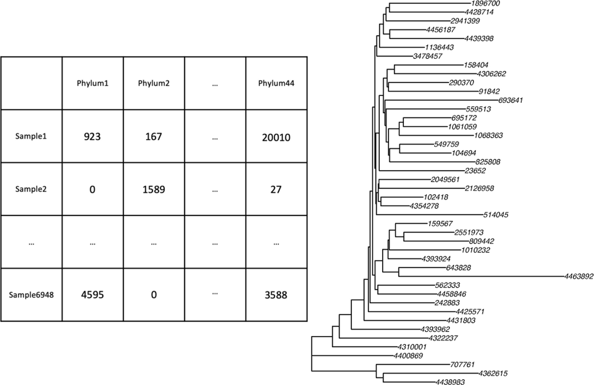
The microbiome read counts table and the corresponding phylogenetic tree of GGMP data aggregated to the phylum level (a high taxonomy level, but the corresponding phylogenetic tree is simple such that it is easier to read here). The numbers on the leaf nodes are the indices of microbes in the established closed-reference tree.

B. Phylogeny-driven neural network (PhyNN)

In this section, we present PhyNN, a composite, locally connected feedforward neural network constructed by scanning the phylogenetic tree from the bottom up with a series of MLPs. Hereinafter, we assume the phylogenetic tree associated with each sample is in a rectangle layout with the root at the top and the leaf nodes at the bottom.

According to phylogenetic principles, clustered microbes that have the same ancestor and similar distance to the root are close in lineage and presumably in characteristics [18]–[20]. Motivated by this fact, we extract the common underlying features for each group of clustered microbes on the leaf nodes by a single model such as MLP. Regarding extracted features of a lower-level clade as a representation of the microbes in that clade, we can repeat this procedure at the higher level and keep moving up until we reach the root to get the final feature for outcome prediction. This procedure takes advantage of both the hierarchy information (the grouped microbes have the same ancestor) and the distance information (the grouped microbes have a similar distance to the root) contained in the phylogenetic tree. Also, the procedure is consistent with the evolution paths depicted in the phylogeny.

Specifically, inspired by CNN that slides over the image and combines pixels by kernels, we propose to horizontally slice the phylogenetic tree into bands, then slide multiple MLPs from the bottom band to the top band, while sequentially integrating the features captured by those MLPs to obtain the final feature for outcome prediction. Define the total height h of a phylogenetic tree as the distance between its lowest leaf node and root. Then, the algorithm of constructing PhyNN is as follows:

1. Starting from the lowest leaf node, slice the tree into K bands with bandwidth b, where K = h/b (the 1st band, a.k.a. the top band, may be narrower than b);

2. To combine nodes from the kth band to the (k − 1)th band, first determine the group of nodes that have the common lowest ancestor in the (k − 1)th band, then integrate their values via an MLP and cache the output to that common ancestor.

3. Repeat 2) until reaching the 1st band.

Note that during the above iterations, we connect the series of MLPs to construct the final PhyNN model – the inputs of an MLP in the (k – 1)th band are the outputs of its linked MLPs and abundances of its linked leaf nodes in the kth band.

We use a toy example with 5 microbes to explain the algorithm in detail. Fig. 2a shows the phylogeny, and Fig. 2b is the PhyNN constructed on it. We walk through the four steps of constructing this PhyNN in Fig. 3:

1. Fig. 3a (Band IV → Band III): Note that Microbe 1 has no ancestors in Band III, so we manually create a pseudo ancestor node for it in Band III. Then, we integrate Microbe 1’s abundance via an MLP, and cache the integrated feature to the pseudo node. Meanwhile, we integrate Microbe 4’s abundance via another MLP, and cache the integrated feature to its ancestor node in Band III.

2. Fig. 3b (Band III → Band II): We further integrate the feature from Microbe 1 via an MLP, and cache the new integrated feature to its ancestor node in Band II. Meanwhile, we integrate Microbes 3 and 5’s abundances and the feature from Microbe 4 via another MLP, and cache the integrated feature to their common ancestor node in Band II.

3. Fig. 3c (Band II → Band I): We integrate the feature from Microbe 1, the feature from Microbes 3,4,5, and Microbe 2’s abundance via an MLP, and cache the integrated feature to the root.

4. Fig. 3d: the feature cached in the root is the final feature extracted by this PhyNN. One may apply different kinds of activation functions on top of it for different prediction tasks (classification or regression).

Fig. 2.

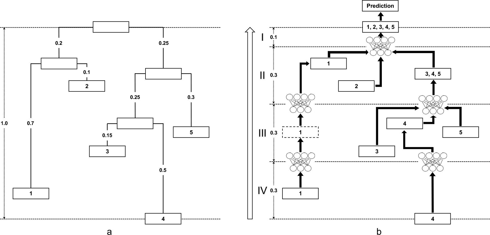
PhyNN constructed on a toy example. a, The toy example has 5 microbes at a certain taxonomy level, and the distance from the lowest leaf node (Microbe 4) to the root is 1.0. Numbers on the branches are their lengths. b, To construct PhyNN, we divide the tree into 4 bands from Microbe 4 to the root with bandwidth b = 0.3, and iteratively integrate nodes in the kth band to the (k − 1)th band along branches via MLPs. The numbers in the nodes represent the microbes of which the information is contained. The information could be the microbes’ abundances (leaf nodes) or outputs of lower level MLPs (internal or created pseudo nodes). The final model that connects all the MLPs along branches is PhyNN.

Fig. 3.

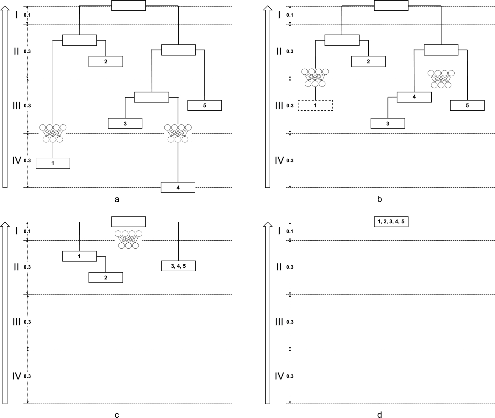
Iterations in constructing PhyNN for the toy example. Traversing the phylogenetic tree from the bottom up (a→b→c→d), we construct the MLPs iteratively from the kth band to the (k − 1)th band.

The PhyNN constructed above is an end-to-end, locally connected architecture. It has two merits. First, it accounts for both the hierarchy and distance information in the phylogeny by sequentially extracting features for each group of clustered microbes via an MLP. Second, the MLPs are connected following the evolution paths in the phylogeny. Thus, PhyNN enables powerful learning that is guided by phylogenetic principles.

C. Formal description of PhyNN construction and training

To formally describe the model construction process introduced above, we need to introduce some notation. Let |S| denote the number of elements in a set S. Let B_k = {N_k1, . . . , N_k|Bk|} denote the set of nodes located in the kth band, where N_kj represents the jth node in the band (j = 1, . . . , |B_k|). Let V (N_kj) be the value cached in node N_kj, which could be a scalar, a vector or NULL (a non-leaf node has no value cached in it). Next, let A(Nkj ) denote the lowest ancestor node of N_kj in B_k−1, which will be NULL if N_kj does not have any ancestor in B_k−1. Then, let S(N_kj) be a set to collect all the nodes in B_k+1 whose lowest ancestor in B_k is N_kj, and we will initialize all such sets as empty sets before starting the algorithm. Finally, let $f_{kj}^{(H)}$ be an MLP with architecture defined by the hyperparameter H. A pseudo code for PhyNN model construction is shown in Algorithm 1.

Algorithm 1.

Construction of PhyNN

Input: Phylogenetic tree T

Bandwidth b

Hyperparameter H for MLP

Divide T into K = ⌈h/b⌉ bands B1, . . ., BK

for k = K to 2 do

for j = 1 to |Bk| do

if A(Nkj) is not NULL then

S(A(Nkj)) ← S(A(Nkj)) ∪ {Nkj}

else

Insert a new (pseudo) node $N_{k-1,\left|B_{k-1}\right|+1}$ to Bk−1 $S\left(N_{k-1,\left|B_{k-1}\right|+1}\right)\leftarrow \left\{N_{kj}\right\}$

end if

end for

for j = 1 to |Bk−1| do

vkj ← NULL vector

for N in S(Nk−1,j) do

if V(N) is not NULL then

vkj ← [vkj, V(N)] (append V(N) to vkj)

end if

end for

if vkj is not NULL vector then

$V\left(N_{k-1,j}\right)\leftarrow f_{kj}^{(H)}\left(v_{kj}\right)$

end if

end for

end for

v11 ← NULL vector

for N in B1 do

if V(N) is not NULL then

v11 ← [v11, V(N)] (append V(N) to v11)

end if

end for

$z\leftarrow f_{11}^{(H)}\left(v_{11}\right)$

Output: The PhyNN model f that accepts the abundances on all leaf nodes as input and yields z as output

In Algorithm 1, each MLP $f_{kj}^{(H)}$ is recursively defined by

$$x^{(q)}=\sigma (W_{kj}^{(q)}{x}^{(q-1)}+b_{kj}^{(q)})q=1,\dots ,Q,$$ (1)

where Q is the number of layers, σ is the activation function, the p^(q) ×p^(q−1) matrix $W_{kj}^{(q)}$ and the p^(q) ×1 vector $b_{kj}^{(q)}$ are the weights and bias to train, x^(q) is a p^(q)×1 column vector, x⁽⁰⁾ corresponds to the input v_kj, and x^(Q) corresponds to the output $f_{kj}^{(H)}\left(v_{kj}\right)$. In addition, the activation function of the last layer of $f_{11}^{(H)}$ is always an identity function, i.e., it is computed by

$$z=x^{(Q)}=W_{11}^{(Q)}{x}^{(Q-1)}+b_{11}^{(Q)}.$$ (2)

The complicated PhyNN model f consisting of many such MLPs $f_{kj}^{(H)}$ will be trained end-to-end as a single model. In other words, all the $f_{kj}^{(H)}$ will be jointly trained together, rather than separately. The trained weights $W_{kj}^{(q)}$ and bias $b_{kj}^{(q)}$ of each $f_{kj}^{(H)}$ will be different, i.e., their weights and bias are not tied, but they have the same architecture defined by the same hyperparameter combination H. In other words, all of these MLPs have the same number of layers Q, the same output dimension p^(Q), and the same hidden dimension p^(q) in each layer, etc., though the input dimension p⁽⁰⁾ of each MLP could be different, as it depends on how many descendent nodes it has in the band below it.

Our model f constructed above can be flexibly applied to different kinds of ML tasks when applying different functions on top of the final output of f. For regression tasks, we apply the identity function and train the model f by minimizing the following mean squared error (MSE) loss

$$L=\frac{1}{n}\sum _{i=1}^n{\Vert y_i-f\left(T_i\right)\Vert }_2^2,$$ (3)

where T_i is the phylogenetic tree of the ith sample with microbial read counts allocated on the leaf nodes and y_i is the clinical outcome of the ith sample. For binary classification tasks, we apply the sigmoid function σ and train the model f by minimizing the following binary cross entropy loss

$$L=\frac{1}{n}\sum _{i=1}^n\left(-y_i\log \left(\sigma \left(f\left(T_i\right)\right)\right)-\left(1-y_i\right)\log \left(1-\sigma \left(f\left(T_i\right)\right)\right)\right)\text{.}$$ (4)

For the ith sample, the predicted probability of Class 1 is given by σ(f(T_i)). For multiple classification tasks with C classes, we apply the softmax function and train the model f by minimizing the following cross entropy loss

$$L=\frac{1}{n}\sum _{i=1}^n\sum _{c=1}^C\left(-y_c\log \left(\mathrm{softmax}{\left(f\left(T_i\right)\right)}_c\right)\right),$$ (5)

where for any C-dimensional vector v = [v₁, . . . , v_C], softmax(v)_c is given by

$$\mathrm{softmax}{(v)}_c=\frac{e^{v_c}}{{\sum }_{c^{\prime }=1}^C{e}^{v_{c^{\prime }}}}.$$

For the ith sample, the predicted probability of the cth class is given by softmax(f(T_i))_c.

Denote all the weights and bias of f as θ. Then with the loss L(θ) defined above, our PhyNN model f is trained with the Adam algorithm [21]. More specifically, at the tth training step, Adam updates the weights and bias of f as follows:

$$\begin{array}{l}{g_t\leftarrow {\nabla }_{\theta }L(\theta )|}_{\theta ={\theta }_{t-1}}\\ m_t\leftarrow {\beta }_1{m}_{t-1}+\left(1-{\beta }_1\right)g_t\\ s_t\leftarrow {\beta }_2{s}_{t-1}+\left(1-{\beta }_2\right)g_t\otimes g_t\\ {\widehat{m}}_t\leftarrow m_t/\left(1-{\beta }_1^t\right)\\ {\widehat{s}}_t\leftarrow s_t/\left(1-{\beta }_2^t\right)\\ {\theta }_t\leftarrow {\theta }_{t-1}-\eta {\widehat{m}}_t/\left(\sqrt{{\widehat{s}}_t}+ϵ\right),\end{array}$$ (6)

where ⊗ denotes the element-wise multiplication, m₀ and s₀ are both initialized as zero vectors, β₁ is a momentum decay hyperparameter that is usually set as 0.9, β₂ is a scaling decay hyperparameter that is usually set as 0.999, ɛ is a smoothing term that is usually set as 10⁻⁸, and η is the learning rate.

D. Deep ensemble learning (DeepEn-Phy)

In the above sections, we only introduce PhyNN with a fixed bandwidth b. The narrower the bandwidth is, the feature at the higher granularity is learned. However, with one bandwidth, we can only learn features at a particular granularity, while features at both high and low granularities could be useful for prediction. Therefore, we propose a deep ensemble method, DeepEn-Phy, to train PhyNN multiple times with a pre-specified sequence of bandwidths and ensemble the results to get the final prediction. Specifically, for classification, we average the predicted probabilities over the various bandwidths and pick the category with the highest average probability as the final prediction; for regression, we average the predicted values over the various bandwidths and use it as the final prediction.

For the sequence of bandwidths, we recommend using an evenly spaced grid in [0, h]. We note that a wider bandwidth may not always incur fewer MLPs than a narrower one (Fig. 4). In general, the complexity of PhyNN decreases as bandwidth increases, but it also depends on the structure of phylogeny. For example, a wide bandwidth may still accidentally cut a large number of branches, resulting in numerous MLPs.

Fig. 4.

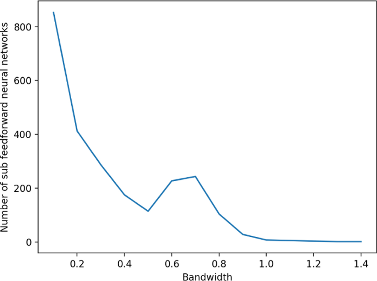
The number of MLPs in PhyNN depends jointly on the bandwidth and the structure of phylogeny. Aggregated to the genus level, the phylogenetic tree of the GGMP data has a total height of h = 1.24. We plot the number of MLPs vs. bandwidth and notice a hump for the medium bandwidths.

E. Data and analysis

We apply DeepEn-Phy to the GGMP data downloaded from the Qiita platform. GGMP is a large microbiome-profiling study conducted in Guangdong Province, China. 7009 stool samples have been collected and processed over 14 districts under the same protocols. The 16S rRNA marker gene (V4 region) was sequenced, and the sequencing reads were processed by QIIME pipeline [22] to obtain the microbiome data. Sociodemographic and biomedical features of the participants have also been collected.

We re-processed the data by QIIME2 pipeline with reference to the 97% Greengenes closed-reference tree [16] and obtained the OTU-level abundances. We then aggregated the OUT-level data to the genus level, i.e., calculated the sum of OTU abundances over all OTUs that map to the same genus-level group. There are 1190 genera in total, and the phylogenetic tree has a total height of h = 1.24. We normalized the microbial read counts by centered log-ratio (CLR, [23], [24]) transformation, which is a usual practice for microbiome data. There are other transformations such as PhILR [25], while we chose CLR for illustration in this paper.

The original paper identified the top 30 host features that are associated with gut microbial variations (Fig. 1b of [17]). The host location showed the strongest association, while the other features have much weaker associations. We select the No.22 and No.9 identified features – smoking status (binary, never smoked=0, ever smoked=1) and BMI (continuous) as the clinical outcomes to predict from the microbial profiles. We randomly split the 7009 samples into training (6000), validation (300), and testing (709) sets, and filtered out the cases with missing smoking status or BMI (Tab. I).

TABLE I.

Summaries of the outcomes of interest in training, validation, and testing sets from the GGMP data.

Smoking status	Never smoked (0)	Ever smoked (1)	Count
Training	4,010	1,937	5,937
Validation	199	99	298
Testing	470	233	703
Overall	4,679	2,269	6,948
BMI	Mean	SD	Count
Training	23.36	3.50	5,915
Validation	23.48	3.66	297
Testing	23.34	3.67	702
Overall	23.37	3.53	6,914

We use Vanilla MLP as a competing method, where all abundances on the leaf nodes are concatenated together as the input and fed to a single fully connected MLP, without considering phylogeny. Another deep learning competing method is PopPhy-CNN, where phylogeny is embedded into CNN. The other four competing methods are random forest, gradient boosting, LASSO, and Ridge.

To make a fair comparison among the deep learning methods, we make their numbers of trainable parameters comparable, because it is a measure for representation capability. For DeepEn-Phy, since h = 1.24, we use six bandwidths b = 0.2, 0.4, 0.6, 0.8, 1.0, 1.2. Then, to predict smoking status, we use 1 hidden layer with 5 neurons in each MLP. The learning rate is 0.005, and a L1 penalization with λ = 0.001 is imposed. To predict BMI, we use 1 hidden layer with 2 neurons in each MLP. The learning rate is 0.005, and a L2 penalization with λ = 0.005 is imposed. For Vanilla MLP, to predict smoking status, we use 9 hidden layers with 90, 80, · · ·, 10 neurons, and the same learning rate and penalization as DeepEn-Phy. To predict BMI, we use 4 hidden layers with 40, 30, · · ·, 10 neurons, and the same learning rate and penalization as DeepEn-Phy. For PopPhy-CNN, we use the authors’ pre-fixed settings [12].

For smoking status, we use the area under the receiver operating characteristic curve (ROC-AUC) to evaluate the classification performance. We also examine the weighted F1-score over the two statuses (calculate F1-score for each status, and calculate their average weighted by the number of true instances for each status [26]). For BMI, we use MSE as the measure to evaluate the prediction performance. Its square root (RMSE) is also reported.

We also obtain the species level data (1606 species), and conduct analysis following the same procedures.

III. Results

Tab. II summarizes the performance of DeepEn-Phy in predicting the binary smoking status and continuous BMI in comparison with the existing methods. We omit PopPhy-CNN in predicting BMI as it is not designed for continuous outcomes. We see that DeepEn-Phy outperforms the others. When predicting smoking status, it increases the ROC-AUC of 0.6813 from the 2nd runner (gradient boosting) to 0.7043, and boosts the F1-score of 0.6439 from the 2nd runner (logistic LASSO) to 0.6839. The corresponding ROC curves are summarized in Fig. 5(left). When predicting BMI, DeepEn-Phy reduces the MSE of 12.9072 from the 2nd runner (random forest) to 12.6812, improving RMSE from 3.5927 to 3.5611.

TABLE II.

Performance of predicting smoking status and BMI from the GGMP microbiome data (genus level).

Smoking Status	ROC-AUC	F1-Score	Time (s)
DeepEn-Phy (nParameter=125,811)	0.7043	0.6839	1,433
Vanilla MLP (nParameter=133,433)	0.6520	0.6346	352
PopPhy-CNN (nParameter=151,618)	0.6163	0.5972	567
Random Forest (nTree=500)	0.6478	0.5409	294
Gradient Boosting (nTree=100)	0.6813	0.6076	11
Logistic LASSO (L1 λ=0.001)	0.6654	0.6439	12
Logistic Ridge (L2 λ=0.001)	0.6422	0.6425	12
BMI	MSE	RMSE	Time (s)
DeepEn-Phy (nParameter=40,038)	12.6812	3.5611	747
Vanilla MLP (nParameter=50,883)	16.6410	4.0793	192
PopPhy-CNN	–	–	–
Random Forest (nTree=500)	12.9072	3.5927	992
Gradient Boosting (nTree=100)	12.9317	3.5961	9
Linear LASSO (L1 λ=0.005)	14.8221	3.8500	10
Linear Ridge (L2 λ=0.005)	28.3400	5.3235	4

Fig. 5.

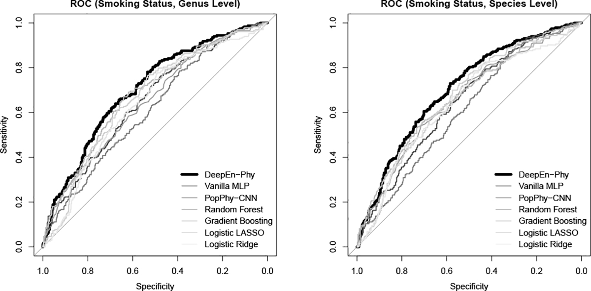
ROC curves for DeepEn-Phy and competing methods when predicting smoking status based on genus level (left) or species level GGMP data (right).

To demonstrate the advantage of DeepEn-Phy over a single PhyNN, we summarize the performance of each of the PhyNNs constructed with different bandwidths (Tab. III). It is shown that in predicting smoking status, none of their ROCAUCs is higher than the ensemble ROC-AUC. Also, in predicting BMI, none of their MSEs is lower than the ensemble MSE. It indicates that the six PhyNNs with different granularities complement each other and boost the final prediction accuracy.

TABLE III.

Performance of the individual PhyNNs in DeepEn-Phy constructed with different bandwidths (genus level).

Smoking status	nMLP	nParameter	ROC-AUC	F1-Score
b = 0.2	412	38,138	0.6931	0.6567
b = 0.4	175	22,958	0.7012	0.6855
b = 0.6	227	26,413	0.6759	0.6254
b = 0.8	104	14,296	0.6910	0.6591
b = 1.0	7	12,053	0.7030	0.4295
b = 1.2	3	11,953	0.6835	0.6672
BMI	nMLP	nParameter	MSE	RMSE
b = 0.2	412	10,057	13.0050	3.6062
b = 0.4	175	6,987	12.8293	3.5818
b = 0.6	227	7,699	13.1785	3.6302
b = 0.8	104	5,693	13.2216	3.6361
b = 1.0	7	4,819	12.9954	3.6049
b = 1.2	3	4,783	13.5238	3.6775

It takes a relatively long time to train DeepEn-Phy because it contains multiple PhyNNs. However, each individual PhyNN is relatively fast to train (smoking status: 239s = 1, 433s/6, BMI: 125s = 747s/6), which is faster than Vanilla MLP (smoking status: 352s, BMI: 192s) and even random forest (smoking status: 294s, BMI: 992s).

On the species level data (Tab. IV), we still observe the dominating performance of DeepEn-Phy. When predicting smoking status, it increases the ROC-AUC of 0.6610 from the 2nd runner (gradient boosting) to 0.7016, and boosts the F1-score of 0.6615 from the 2nd runner (logistic Ridge) to 0.6748. The corresponding ROC curves are summarized in Fig. 5(right). When predicting BMI, DeepEn-Phy reduces the MSE of 12.7475 from the 2nd runner (random forest) to 12.5559, improving RMSE from 3.5704 to 3.5434. Also, none of the individual PhyNNs shows better performance than DeepEn-Phy, which again demonstrates the superiority of ensemble learning (Tab. V).

TABLE IV.

Performance of predicting smoking status and BMI from the GGMP microbiome data (species level).

Smoking Status	ROC-AUC	F1-Score	Time (s)
DeepEn-Phy (nParameter=158,166)	0.7016	0.6748	2,213
Vanilla MLP (nParameter=171,289)	0.6471	0.6383	652
PopPhy-CNN (nParameter=238,658)	0.6122	0.5946	833
Random Forest (nTree=500)	0.6583	0.5409	408
Gradient Boosting (nTree=100)	0.6610	0.5887	14
Logistic LASSO (L1 λ=0.001)	0.6600	0.6491	19
Logistic Ridge (L2 λ=0.001)	0.6445	0.6615	17
BMI	MSE	RMSE	Time (s)
DeepEn-Phy (nParameter=51,636)	12.5559	3.5434	1,211
Vanilla MLP (nParameter=67,939)	16.3519	4.0437	346
PopPhy-CNN	–	–	–
Random Forest (nTree=500)	12.7475	3.5704	1,325
Gradient Boosting (nTree=100)	12.7675	3.5732	12
Linear LASSO (L1 λ=0.005)	15.1966	3.8983	38
Linear Ridge (L2 λ=0.005)	21.1825	4.6024	6

TABLE V.

Performance of the individual PhyNNs in DeepEn-Phy constructed with different bandwidths (species level).

Smoking Status	nMLP	nParameter	ROC-AUC	F1-Score
b = 0.2	472	46,148	0.6762	0.6599
b = 0.4	192	28,248	0.6827	0.6230
b = 0.6	263	32,938	0.6992	0.6739
b = 0.8	104	18,506	0.6738	0.6613
b = 1.0	7	16,213	0.6915	0.3297
b = 1.2	3	16,113	0.6892	0.5370
BMI	nMLP	nParameter	MSE	RMSE
b = 0.2	472	12,573	13.1659	3.6285
b = 0.4	192	8,925	13.0051	3.6063
b = 0.6	263	9,847	13.0441	3.6117
b = 0.8	104	7,361	12.7841	3.5755
b = 1.0	7	6,483	13.6776	3.6983
b = 1.2	3	6,447	14.1868	3.7665

IV. Conclusion

The microbiome is a critical biomarker to predict host disease status and clinical outcomes. Although it is shown that incorporating phylogeny information will improve the prediction accuracy, few approaches take direct and full advantage of the phylogeny as it requires challenging feature engineering. Deep learning achieves automatic feature extraction and powerful approximation to complicated functions, so it is a promising tool for microbiome prediction involving phylogeny.

We propose DeepEn-Phy, an ensemble method based on a novel phylogeny-driven deep neural network, PhyNN, to predict a host’s categorical or continuous clinical outcomes from the microbial profiles. We slice the phylogenetic tree from the lowest leaf node to the root by a pre-specified bandwidth. Then, from the bottom up, we recursively integrate the nodes that share the common lowest ancestor in the upper band via an MLP. The final PhyNN model is constructed by connecting all the MLPs. Further, we ensemble multiple PhyNNs, each of which uses different bandwidths, to get the final prediction.

The real case study on the GGMP data shows that DeepEn-Phy outperforms the existing ML and deep learning methods in predicting smoking status (binary) and BMI (continuous) from the microbiome data. Investigating the performance of each of the individual PhyNNs in DeepEn-Phy, we confirm that the ensemble step helps to boost the final prediction accuracy. In the future, we will use more data sets and more interesting clinical outcomes such as disease status to further validate the advantages of DeepEn-Phy.

Although DeepEn-Phy is developed within the microbiome context, it is also applicable to other huge and complicated hierarchical or directional data. Such data can be found in genetics and genomics, metabolomics, demographics with housing data, etc. Therefore, DeepEn-Phy is a general deep learning approach that could be used in many real-life applications.

Another extension is that we can regard each PhyNN with a pre-specified bandwidth as an encoder to encode important information in its output vector. Then, we can use these encoding vectors in another ML or deep learning model, e.g., linear models, to calibrate the final prediction.

One more interesting direction is to develop an effective algorithm to identify the important microbes for a particular host clinical outcome. Although interpretability of deep learning models is a challenging topic, we believe that the locally connected nature of PhyNN could help us detect the important microbes.

Overall, DeepEn-Phy sheds light on designing deep neural network architectures within the context of phylogeny-constrained microbiome data, or more generally the graph-based microbiome data. Essentially, the proposed PhyNN is similar to a one-layer Graph Neural Network (GNN) [27] designed for graph-level prediction. The main idea of GNN is to iteratively update the representation of each node in the graph by combining the representations of its neighbors. One of the key differences between PhyNN and GNN is that PhyNN takes account of the structure of the phylogenetic tree and underlying phylogenetic principles when deciding which neighbors it will use to combine, but GNN will simply use all the neighbors of a node to combine. Moreover, PhyNN updates the node representations sequentially from leaves to the root of the tree and uses the root representation as the graph representation, but GNN on such a homogeneous graph will treat all nodes equally, update all node representations simultaneously, and aggregate all the final node representations to form the graph representation. Due to its connection with GNN, we believe the architecture of PhyNN can be further optimized by utilizing common techniques used in GNN. Moreover, we believe DeepEn-Phy opens an avenue for applying a GNN-like model to capture the complex information and dependency in graph-based microbiome data.

References

- [1].Morgan XC and Huttenhower C, “Chapter 12: Human microbiome analysis,” PLoS computational biology, vol. 8, no. 12, p. e1002808, 2012. [DOI] [PMC free article] [PubMed] [Google Scholar]
- [2].Wang J and Jia H, “Metagenome-wide association studies: fine-mining the microbiome,” Nature Reviews Microbiology, vol. 14, no. 8, p. 508, 2016. [DOI] [PubMed] [Google Scholar]
- [3].Claus SP, Guillou H, and Ellero-Simatos S, “The gut microbiota: a major player in the toxicity of environmental pollutants?” Npj biofilms and microbiomes, vol. 2, no. 1, pp. 1–11, 2016. [DOI] [PMC free article] [PubMed] [Google Scholar]
- [4].Qin J, Li Y, Cai Z, Li S, Zhu J, Zhang F, Liang S, Zhang W, Guan Y, Shen D et al. , “A metagenome-wide association study of gut microbiota in type 2 diabetes,” Nature, vol. 490, no. 7418, pp. 55–60, 2012. [DOI] [PubMed] [Google Scholar]
- [5].Mitchell CM, Srinivasan S, Zhan X, Wu MC, Reed SD, Guthrie KA, LaCroix AZ, Fiedler T, Munch M, Liu C et al. , “Vaginal microbiota and genitourinary menopausal symptoms: a cross sectional analysis,” Menopause (New York, NY), vol. 24, no. 10, p. 1160, 2017. [DOI] [PMC free article] [PubMed] [Google Scholar]
- [6].Zhu Q, Huo B, Sun H, Li B, and Jiang X, “Application of deep learning in microbiome,” Journal of Artificial Intelligence for Medical Sciences, vol. 1, no. 1–2, pp. 23–29, 2020. [Google Scholar]
- [7].Tibshirani R, “Regression shrinkage and selection via the lasso,” Journal of the Royal Statistical Society: Series B (Methodological), vol. 58, no. 1, pp. 267–288, 1996. [Google Scholar]
- [8].Marcos-Zambrano LJ, Karaduzovic-Hadziabdic K, Loncar Turukalo T, Przymus P, Trajkovik V, Aasmets O, Berland M, Gruca A, Hasic J, Hron K et al. , “Applications of machine learning in human microbiome studies: a review on feature selection, biomarker identification, disease prediction and treatment,” Frontiers in microbiology, vol. 12, p. 313, 2021. [DOI] [PMC free article] [PubMed] [Google Scholar]
- [9].Bengio Y, Courville A, and Vincent P, “Representation learning: A review and new perspectives,” IEEE transactions on pattern analysis and machine intelligence, vol. 35, no. 8, pp. 1798–1828, 2013. [DOI] [PubMed] [Google Scholar]
- [10].Hornik K, “Approximation capabilities of multilayer feedforward networks,” Neural networks, vol. 4, no. 2, pp. 251–257, 1991. [Google Scholar]
- [11].Ditzler G, Polikar R, and Rosen G, “Multi-layer and recursive neural networks for metagenomic classification,” IEEE transactions on nanobioscience, vol. 14, no. 6, pp. 608–616, 2015. [DOI] [PubMed] [Google Scholar]
- [12].Reiman D, Metwally AA, Sun J, and Dai Y, “Popphy-cnn: a phylogenetic tree embedded architecture for convolutional neural networks to predict host phenotype from metagenomic data,” IEEE journal of biomedical and health informatics, vol. 24, no. 10, pp. 2993–3001, 2020. [DOI] [PubMed] [Google Scholar]
- [13].Rideout JR, He Y, Navas-Molina JA, Walters WA, Ursell LK, Gibbons SM, Chase J, McDonald D, Gonzalez A, Robbins-Pianka A et al. , “Subsampled open-reference clustering creates consistent, comprehensive otu definitions and scales to billions of sequences,” PeerJ, vol. 2, p. e545, 2014. [DOI] [PMC free article] [PubMed] [Google Scholar]
- [14].Bolyen E, Rideout JR, Dillon MR, Bokulich NA, Abnet CC, Al-Ghalith GA, Alexander H, Alm EJ, Arumugam M, Asnicar F et al. , “Reproducible, interactive, scalable and extensible microbiome data science using qiime 2,” Nature biotechnology, vol. 37, no. 8, pp. 852–857, 2019. [DOI] [PMC free article] [PubMed] [Google Scholar]
- [15].Callahan BJ, McMurdie PJ, Rosen MJ, Han AW, Johnson AJA, and Holmes SP, “Dada2: high-resolution sample inference from illumina amplicon data,” Nature methods, vol. 13, no. 7, pp. 581–583, 2016. [DOI] [PMC free article] [PubMed] [Google Scholar]
- [16].DeSantis TZ, Hugenholtz P, Larsen N, Rojas M, Brodie EL, Keller K, Huber T, Dalevi D, Hu P, and Andersen GL, “Greengenes, a chimera-checked 16s rrna gene database and workbench compatible with arb,” Applied and environmental microbiology, vol. 72, no. 7, pp. 5069–5072, 2006. [DOI] [PMC free article] [PubMed] [Google Scholar]
- [17].He Y, Wu W, Zheng H-M, Li P, McDonald D, Sheng H-F, Chen M-X, Chen Z-H, Ji G-Y, Mujagond P et al. , “Regional variation limits applications of healthy gut microbiome reference ranges and disease models,” Nature medicine, vol. 24, no. 10, pp. 1532–1535, 2018. [DOI] [PubMed] [Google Scholar]
- [18].Fitch WM and Margoliash E, “Construction of phylogenetic trees,” Science, vol. 155, no. 3760, pp. 279–284, 1967. [DOI] [PubMed] [Google Scholar]
- [19].Janda JM and Abbott SL, “16s rrna gene sequencing for bacterial identification in the diagnostic laboratory: pluses, perils, and pitfalls,” Journal of clinical microbiology, vol. 45, no. 9, pp. 2761–2764, 2007. [DOI] [PMC free article] [PubMed] [Google Scholar]
- [20].Petti C, Polage CR, and Schreckenberger P, “The role of 16s rrna gene sequencing in identification of microorganisms misidentified by conventional methods,” Journal of clinical microbiology, vol. 43, no. 12, pp. 6123–6125, 2005. [DOI] [PMC free article] [PubMed] [Google Scholar]
- [21].Kingma DP and Ba J, “Adam: A method for stochastic optimization,” arXiv preprint arXiv:1412.6980, 2014. [Google Scholar]
- [22].Caporaso JG, Kuczynski J, Stombaugh J, Bittinger K, Bushman FD, Costello EK, Fierer N, Peña AG, Goodrich JK, Gordon JI et al. , “Qiime allows analysis of high-throughput community sequencing data,” Nature methods, vol. 7, no. 5, pp. 335–336, 2010. [DOI] [PMC free article] [PubMed] [Google Scholar]
- [23].Quinn TP, Erb I, Gloor G, Notredame C, Richardson MF, and Crowley TM, “A field guide for the compositional analysis of anyomics data,” GigaScience, vol. 8, no. 9, p. giz107, 2019. [DOI] [PMC free article] [PubMed] [Google Scholar]
- [24].Quinn TP, Crowley TM, and Richardson MF, “Benchmarking differential expression analysis tools for rna-seq: normalization-based vs. log-ratio transformation-based methods,” BMC bioinformatics, vol. 19, no. 1, pp. 1–15, 2018. [DOI] [PMC free article] [PubMed] [Google Scholar]
- [25].Silverman JD, Washburne AD, Mukherjee S, and David LA, “A phylogenetic transform enhances analysis of compositional microbiota data,” Elife, vol. 6, p. e21887, 2017. [DOI] [PMC free article] [PubMed] [Google Scholar]
- [26].Bisong E, “Introduction to scikit-learn,” in Building Machine Learning and Deep Learning Models on Google Cloud Platform. Springer, 2019, pp. 215–229. [Google Scholar]
- [27].Wu L, Cui P, Pei J, Zhao L, and Song L, “Graph neural networks,” in Graph Neural Networks: Foundations, Frontiers, and Applications. Springer, 2022, pp. 27–37. [Google Scholar]