AMBER Drug Discovery Boost tools: Automated workflow for production free energy simulation setup and analysis (ProFESSA)

Abstract

We report an automated workflow for production free energy simulation setup and analysis (ProFESSA) using the GPU-accelerated AMBER free energy engine with enhanced sampling features and analysis tools part of the AMBER Drug Discovery Boost package that have been fully integrated into the AMBER22 release. The workflow establishes a flexible, end-to-end pipeline for performing alchemical free energy simulations that brings to bear technologies, including new enhanced sampling features and analysis tools, to practical drug discovery problems. ProFESSA provides the user with top-level control of large sets of free energy calculations, and offers access to the following key functionalities: 1) automated setup of file infrastructure; 2) enhanced conformational and alchemical sampling with the ACES method; 3) network-wide free energy analysis with optional imposition of cycle closure and experimental constraints. The workflow is applied to perform absolute and relative solvation free energy and relative ligand-protein binding free energy calculations using different atom-mapping procedures. Results demonstrate the workflow is internally consistent and highly robust. Further, application of new network-wide Lagrange multiplier constraint analysis that imposes key experimental constraints substantially improves binding free energy predictions.

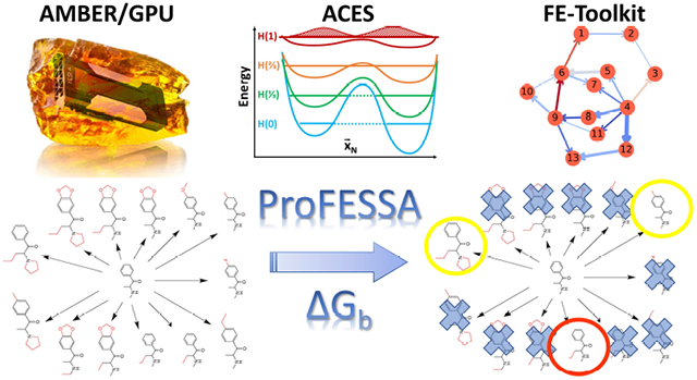
Graphical Abstract

1. Introduction

Alchemical free energy (AFE) simulations have become an indispensable tool in computer-aided drug discovery.^1-7 In recent years, simultaneous advancement in computer hardware, simulation software, and free energy methods has enabled highly efficient and increasingly accurate GPU-accelerated AFE simulations to address a broad scope of real world drug discovery applications.^2,8-14 AFE simulations rely on physics-based atomistic models and statistical-mechanics methods,^1,6,13,15 and leverage the property that the free energy is a state function to enable non-physical thermodynamic pathways to be constructed that are more amenable to practical computation. AFE simulations are used in a wide range of contexts,¹⁵ but for the purposes of the current work, focus will be placed on the calculation of absolute and relative solvation (ASFE and RSFE) and binding (ABFE and RBFE) free energies that are of primary importance to computer aided drug discovery.^{1,12,13,16,17}

Pharmaceutical companies routinely use GPU-accelerated AFE calculations to design potency and selectivity to circumvent off-target affects and guide the prioritization of compounds for synthesis and testing in the lead optimization cycle.^{1,12,13,16,17} Over the last several years, our lab has spearheaded the development of GPU-accelerated free energy simulation and analysis methods in AMBER^1,9,10,18-23 and FE–ToolKit^24-26 and provided advanced beta testing access to academic and industry partners through the AMBER Drug Discovery Boost (AMBER DD Boost) package¹² to facilitate method validation before it’s integration into the official AMBER release versions. Among these have been the development of smoothstep softcore potentials and the introduction of flexible user control of interactions that enables optimization of alchemical transformation pathways,^21,27 new alchemical enhanced sampling method (ACES)²⁸ (see description in Supporting Information) to avoid kinetic traps and overcome local “hot-spot” problems in the λ dimension, and the release of FE–ToolKit to provide a robust set of network-wide free energy analysis tools that includes imposition of cycle closure and experimental constraints.^24-26 The goal of the current work is to report a new automated workflow for production free energy simulation setup and analysis (ProFESSA) using the GPU-accelerated AMBER free energy engine that integrates these new features, methods and analysis tools.

Setting up of AFE calculations consists of a series of technical, detail-oriented steps that are mistake-prone. Moreover, practical drug discovery applications such as lead optimization cycles may require several hundred independent calculations, each run with identical settings to allow for maximum error cancellations and highest predictive accuracy. This makes automation an absolute necessity. Numerous tools have been developed that help facilitate automation of various stages of AFE calculations, such as generation of initial input, parameter and topology files,^29-32 mapping out favorable alchemical pathways,,³³ and analysis of production simulations.³⁴ Several robust and validated workflows that provide different levels of automation along the end-to-end pipeline for AFE calculations also exist,^23,32,35-37 the most notable being the commercially available FEP+ from Schrödinger that enables setup, execution, and analysis of AFE calculations.³⁸ Very recently, other non-commercial workflows have been reported, including FEPrepare,³⁹ a web-based tool for automated setup of RBFE calculations using NAMD, PyAutoFEP,⁴⁰ an open-source tool that enables automated setup and analysis of AFE simulations using GROMACS, and BAT.py,⁴¹ a tool for automation of ABFE calculations for docking refinement and compound evaluation.

Herein, we introduce a flexible, end-to-end pipeline for performing AFE simulations using AMBER that brings to bear new technologies that we have developed as part of AMBER DD Boost, to practical drug discovery problems. This pipeline, referred to as ProFESSA (Production Free Energy Simulation Setup and Analysis), automates and optimizes the various laborious and time-consuming steps that are involved in the setup, equilibration and production/data collection, and analysis of ASFE, RSFE, and RBFE calculations using AMBER/AMBER DD Boost (Figure 1). ProFESSA uses a simplified input file that provides the user with top-level control over the intended AFE calculations, and offers the following key functionalities:

Figure 1:

ProFESSA : An Automated workflow for Production Free Energy Simulation Setup and Analysis.

• Automated setup of file infrastructure - For a given network of transformations, the setup module of ProFESSA facilitates:

  • Generation of “single-topology” parameter and coordinate files starting from crystal structures
  • Generation of common core and softcore regions for individual transformations using multiple atom-mapping algorithms
  • Generation of necessary AMBER input files and job submission scripts
• Enhanced conformational and alchemical sampling - ProFESSA brings together several of our recent methodological advances in enhanced sampling techniques to accelerate convergence in free energy (or regular MD) simulations, and improve precision of predicted ligand binding free energies. Specifically, the workflow enables the use of:

  • ACES method²⁸ as a tool to increase sampling along the coordinates that are most relevant to a given transformation
  • 2-state simulation setup in conjunction with HREMD to improve sampling and maintain equilibrium between windows along the entire λ dimension
  • Robust equilibration and production protocol to alleviate initial conformational bias

• Seamless network-wide analysis - ProFESSA’s analysis module processes the simulation output files and uses BARnet and MBARnet methods to enable network-wide analysis of binding free energies with or without imposition of cycle closure and experimental constraints.

The remainder of the article is organized as follows: In section 2, we summarize the key functionalities of ProFESSA; in section 3, we provide details of the computational methods; in section 4, we present results and discussion for a series of illustrative test cases and comparison of results from calculations with several different simulation settings; lastly, in section 5 we conclude by recapitulating the key developments in this work, and discussing future direction.

2. Key Features of ProFESSA

The ProFESSA workflow has several practical and innovative features that enable robust production free energy simulations:

• Automated atom mapping between reference and target ligands using MCS, MCS-E and MCS-E_nw algorithms.

• Automated generation of topology and starting configuration files.

• Thermodynamic integration and free energy perturbation simulations using AMBER GPU-accelerated MD engine.

• Integration of consistent real-state endpoint simulations for each ligand into 2-state Hamiltonian replica exchange framework.

• Enhanced sampling with REST2 and new ACES methods.

• Robust network-wide analysis using MBARnet and BARnet with cycle closure and experimental constraints.

• Detailed reporting of statistical/error/network stability indexes for free energy estimates using FE-ToolKit.

The ProFESSA workflow integrates these recently developed features, methods and analysis tools, some of which are presented here for the first time such as network stability (Lagrange multiplier) indexes discussed below.

2.1. The ProFESSA input file

The ProFESSA input file (Figure S1 in Supporting Information), which is distinct from AMBER input files, is designed to provide the user with top-level control over the key aspects of ASFE/RSFE/RBFE calculations, while automating the laborious and time-consuming intermediate steps. The input file consists of a series of sections, where each section corresponds to a particular aspect of performing the AFE calculations. In the section Intended calculations, the user must specify a directory that contains the initial structure and parameter files that include for each ligand its mol2, frcmod, and lib files, and a PDB file of the protein-ligand complex, list of transformations or edges, and the number of lambda windows to be used in the RBFE simulations. Note that the component for generating ligand parameters is not included within the workflow. The user can either use antechamber and parmchk2 packages, which ship with AmberTools, to generate GAFF^10,42 or GAFF2⁴³ frcmod files for each ligand, or use their own defined force field files. In near future, the generation of ligand paramaters will be implemented and integrated with the ProFESSA workflow. In the section Action of the workflow the user specifies whether the workflow will be used for setup or analysis. In the section Identification of softcore and common core regions, the user can choose among several algorithms for automatic determination of the softcore and common core regions for the various specified edges. In the section Preparation of MD simulation boxes the user has the option of specifying details related to the preparation of AMBER format MD boxes from the initial input files. The user can specify protein force field to ff14SB⁴⁴ or ff19SB via pff, ligand force field to GAFF^10,42 or GAFF2⁴³ via lff, and water model to TIP3P⁴⁵ or TIP4P-Ew⁴⁶ via wm. In the sections TI simulation setup and TI simulation details, the user can specify how the equilibration protocol will be set up and the key parameters that will be used in the RBFE simulations. In the section Job submission scripts, the user can specify details related to job submission scripts, and lastly in the section Analysis, the user can specify details related to the analysis of the RBFE simulations using FE–ToolKit.

2.2. Automated generation of common core (CC) and softcore (SC) regions

A critical step in the setup of a ASFE/RSFE/RBFE simulation is the one-to-one mapping of equivalent atoms in the reference and target ligand molecules that defines the common core (CC) and softcore (SC) regions.²⁷ Defining the CC and SC regions manually is a simple task when performing a handful of these calculations between similar ligands but becomes increasingly tedious as the transformation network increases in size and complexity, and can become very time consuming and lead to human error. ProFESSA enables the automatic generation of the CC and SC regions associated with the various desired transformations with options of choosing three different algorithms, referred to as MCS, MCS-E, and MCS-E_nw (Figure 2). MCS corresponds to the use of the Maximum Common Substructure search algorithm⁴⁷ as implemented in the Cheminformatics software RDKit.⁴⁸ MCS uses a similarity criterion to decide if an atom or bond matches between two structures and aims to identify their maximum overlap. MCS, while widely used in context of automated alchemical free energy simulations, in its original form may not always be suitable, particularly in cases where atom mapping based on “maximum overlap” is not desired, and may lead to unstable TI simulations or cycle closure issues. MCS-E (or “extended” MCS) is an atom-mapping algorithm we developed that builds on the original MCS algorithm and excludes from the “maximum overlap” region that is identified purely from structural similarity; i.e. atoms that differ either in chemical identity or hybridization. This extension leads to more stable TI simulations. MCS-E_nw corresponds to a variant of MCS-E which ensures that the CC and SC regions of each unique ligand molecule are identical in all transformations in which the ligand participates within the given network (nw). MCS-E_nw is currently only available in AMBER DD Boost but will be incorporated into a future AMBER release. Such a definition, along with setting up each system automatically with identical number of solvent particles, would enable new network-wide enhanced sampling methods to be used where HREMD could be performed to exchange between simulations along different edges of the thermodynamic graph.

Figure 2:

Illustration of the MCS, MCS-E, and MCS-E_nw algorithms for identification of SC and CC regions. Both panels (A) and (B) illustrate the edges that form the dense thermodynamic graph with Cdk2 ligands. SC regions identified by the MCS and MCS-E algorithms are indicated in panel (A) by red and blue circles, respectively, while SC regions identified my the MCS-E_nw algorithm are indicated in panel (B) are indicated by green circles.

2.3. Automated generation of topology and starting configuration files

RSFE/RBFE simulations on a network of transformations (or ASFE simulations on a library of molecules) require the MD simulation boxes for the various TI calculations to be prepared in a consistent fashion, ideally with an identical number of solvent molecules, such that they are inter-operable with HREMD and ACES simulations for a given transformation. Our workflow can, in an automated way, generate all the necessary topology and configuration files using user-defined force field, water and ion models, box size and shape, ion concentration, and if specified, containing identical number of water molecules and ions. Moreover, the workflow has the flexibility to generate the topologies with and without hydrogen mass repartitioning (HMR) to enable longer MD time steps.

The initial configuration files for a given RSFE/RBFE calculation can be generated in two different ways. In the conventional approach, referred to here as the 1-state model (and has up until now been the only practical option in AMBER), only the reference ligand structure (in the case of RSFE) or receptor-reference ligand complex structure (in case of RBFE) is considered and corresponds to the λ=0 state (and the λ=1 state is extrapolated/built from the λ=0 state), while in the 2-state model introduced here, both the reference and target ligand structures (in case of RSFE) or receptor-reference ligand and receptor-target ligand complex structures (in case of RBFE) are considered and correspond to the λ=0 state and λ=1 state, respectively. The latter is particularly useful if the conformation of the receptor is significantly different in the receptor-reference and receptor-target complexes.

2.4. Automated generation of AMBER DD Boost input files for a robust equilibration protocol

Sufficient equilibration of starting structures is essential, particularly for accurate and precise RBFE predictions. ProFESSA utilizes an exhaustive and carefully chosen equilibration protocol illustrated in Figure 3 and generates the input file infrastructure necessary for running equilibration and production simulations. Equilibration simulations are divided into two phases; the first phase consists of rigorous equilibration of only the λ=0 state in the case of the 1-state model and both λ=0 and λ=1 states for the 2-state model. This is followed by the second phase in which all λ states are generated and equilibrated independently. In the case of the 1-state model, all λ states are generated from the equilibrated λ=0 state, while in the case of the 2-state model, the first half of the λ windows are generated from the equilibrated λ=0 state and the other half of the λ windows are generated from the equilibrated λ=1 state. Note: the 1-state model often leads to hysteresis when the reference and target ligands are switched, as this will change the starting conditions for the equilibration. For the 2-state model, initial conditions considering both end states symmetrically eliminate hysteresis. Production simulations are initiated from the structures obtained at the end of the equilibration. The workflow allows top-level control on the production simulation parameters, such as simulation length, time step, use of replica exchange and ACES, and flags that are specific to AMBER DD Boost. The workflow also gives the user flexibility to skip some parts of the equilibration procedure, which the user can comment-out some parts of the equilibration procedure in the default slurm script, or provide their own slurm script.

Figure 3:

Equilibration protocols used within the ProFESSA workflow.

3. Methods

All free energy calculations were performed using concerted transformation pathways, and a recently developed smoothstep softcore potential²⁷ introduced in AMBER22.⁴⁹ The functional form of this softcore potential includes an universal pairwise interaction with consistent power scaling of Coulomb and Lennard-Jones interactions with unitless control parameters and rigorous smoothing of the potential at the non-bonded cut-off boundary. The different classes of example systems were not all run using exactly the same procedures or force fields. For example, for the hydration free energy simulations the GAFF force field is used with TIP3P water to enable consistent comparisons with work of others,^50,51 and a 1 fs time step was used, rather than the more common 2 fs and 4 fs time steps when SHAKE is used with hydrogen mass repatitioning.^52,53 In other cases, the more recent GAFF2 force field was used with TIP4PEw water model as is more commonly employed by the authors.

3.1. Absolute and relative hydration free energy simulations

We performed absolute and relative hydration free energy calculations for several molecules taken from FreeSolv database.⁵⁴ Initial structures were taken from FreeSolv⁵⁴ and simulations were prepared using the ProFESSA workflow. For the small molecules, the GAFF force field^10,42 parameters along with AM1-BCC charges^55,56 were used. The systems were solvated with TIP3P⁴⁵ water and an initial buffer size of 20 Å. Any remaining net charge of the system was first neutralized and then solvated as 0.15 M ion concentration by addition of Na⁺ or Cl⁻ ions (modeled using force field parameters of Joung and Cheatham⁵⁷) as appropriate. Four independent trials of each simulation were performed by using different random number seeds to adjust the initial conditions. In the 2-state simulation setup, as a first step the solvated MD boxes for all systems were generated, the system with the fewest number of water molecules and ions was identified, and then appropriate number of water molecules and ions, lying toward the outer edge of the MD boxes, were deleted from all other systems such that all systems end up with identical number of water molecules and ions (this is done automatically in the ProFESSA workflow). The equilibration protocol used was analogous to that described in Figure 3. The production free energy calculations were performed using 25 λ windows, spaced as per the S2 schedule along the λ dimension ranging from 0 to 1 (0.0, 0.1768, 0.2298, 0.2694, 0.3027, 0.3323, 0.3594, 0.3849, 0.4091, 0.4325, 0.4553, 0.4777, 0.5, 0.5223, 0.5447, 0.5675, 0.5909, 0.6151, 0.6406, 0.6677, 0.6973, 0.7306, 0.7702, 0.8232, 1.0). Each window was run in the NPT ensemble at 300 K using the Langevin thermostat with a friction constant of 2.0 ps⁻¹ for 5 ns. The long-range electrostatics were evaluated with the particle mesh Ewald (PME) method.^58,59 A cutoff of 10 Å was used for non-bonded interactions, including the direct space PME terms and particles interacting through softcore potentials. Only the bonds involving hydrogen were constrained with the SHAKE algorithm^60,61 except the atoms of ligands, and all simulations were performed using a 1 fs integration time step.

3.2. Relative binding free energy simulations

We examined six possible transformations between four ligands that target binding to protein Cyclin-dependent kinase 2 (Cdk2).^38,62 The specific ligands chosen in this study were 1h1q, 1h1r, 1oiu, and 1h1s. Initial structures were taken from the published data and simulations were prepared using ProFESSA workflow, using the AMBER ff14SB⁴⁴ force field for proteins, GAFF2⁴³ for ligands, TIP4P-Ew⁴⁶ for water molecules. An initial buffer size of 20 and 16 Å were used for the aqueous and protein-ligand complex leg simulations, respectively. Three independent trials of each simulation were performed by using different random number seeds to adjust the initial conditions. In the 2-state simulation setup, as a first step the solvated MD boxes for all systems were generated, the system with the fewest number of water molecules and ions was identified, and then appropriate number of water molecules and ions, lying toward the outer edge of the MD boxes, were deleted from all other systems such that all systems end up with identical number of water molecules and ions. The equilibration protocol used is described in Figure 3. The production free energy calculations were performed using 25 λ windows, spaced as per the S2 schedule along the λ dimension ranging from 0 to 1 (0.0, 0.1768, 0.2298, 0.2694, 0.3027, 0.3323, 0.3594, 0.3849, 0.4091, 0.4325, 0.4553, 0.4777, 0.5, 0.5223, 0.5447, 0.5675, 0.5909, 0.6151, 0.6406, 0.6677, 0.6973, 0.7306, 0.7702, 0.8232, 1.0). The S2 scheduling is chosen ti guarantee the excellent replica exchange ration between λ windows, and to get the converge free energy results. The optimal λ scheduling will be expored in details in the future study. Each window was run in the NPT ensemble at 300 K using the Langevin thermostat with a friction constant of 2.0 ps⁻¹ for 5 ns. The long-range electrostatics were evaluated with the particle mesh Ewald (PME) method.^58,59 A cutoff of 10 Å was used for non-bonded interactions, including the direct space PME terms and particles interacting through softcore potentials. Only the bonds involving hydrogen were constrained with the SHAKE algorithm^60,61 except the atoms of ligands, and all simulations were performed using a 1 fs integration time step.

4. Results and Discussion

Here we provide demonstrations of the use of the workflows to run alchemical free energy simulations using various new features including ACES enhanced sampling, 2-state Hamiltonian replica-exchange and ACES setup, and network-wide free energy analysis. The workflows are applied to examine absolute and relative solvation free energies of small molecules and relative binding free energies of ligand-protein complexes.

In order to facilitate these comparisons, we introduce an abbreviated notation that is used in the figures, tables and discussion: “SC2/R” and “SC2/N” indicates a gti_add_sc flag value of 2, with (SC2/R) and without (SC2/N) HREMD, respectively. The gti_add_sc flag controls the internal energy terms that are scaled by λ in the dummy state, and a value of 2 scales all electrostatic interaction, but maintains all internal bonded (including torsion angle) and Lennard-Jones (LJ) terms (except 1-4 LJ terms that are strongly coupled with the torsion angles). A gti_add_sc value of 5 also scales torsion terms around rotatable single bonds, which creates an “enhanced sampled” dummy state. ACES uses this enhanced sampled dummy state along with HREMD. The ACES method has been described in detail elsewhere, and demonstrated to have advantages over other REST2-like implementations.²⁸

4.1. Alchemical Enhanced Sampling with ACES using 2-state HREMD setup

2-state Hamiltonian replica exchange/ACES setup.

Setup of the Hamiltonian replica exchange framework for intermediate alchemical states in RBFE simulations is important. Within the limit of infinite sampling, results should not be sensitive to these initial conditions, but in practice the setup is very important. As discussed above, traditionally in AMBER setup of HREMD simulations for λ > 0 values would be determined from the structure of the λ = 0 state. Results would differ statistically in the ligands were reversed (hysteresis effect). In the 2-state approach both real state endpoint structures are considered simultaneously and intermediate states are created symmetrically in the HREMD setup. This eliminates problems of hysteresis as the setup and sampling are invariant to permutation of the ligands.

Here we demonstrate the use of ACES as robust alchemical enhanced sampling method. We focus on absolute and relative solvation free energies as these calculations do not require other features of the workflow such as 2-state Hamiltonian replica exchange setup. This provides a set of test cases that allows us to focus more on the ACES approach itself. A detailed description of the ACES approach and more comprehensive tests have been presented elsewhere.²⁸ We chose a set of molecules examined previously in AMBER validation studies,²⁰ and selected from the FreeSolv⁵⁴ database (v0.51) for which the reported deviations between the calculated AMBER/GAFF and experimental solvation free energies (calculated using a different protocol described in published work^50,51) are anomalously large²⁸ (Table 1).

Table 1:

Comparsion of absolute hydration free energy values (kcal/mol) for selected Free-Solv entries and molecules examined previously for AMBER validation with different simulation protocols, along with the experimental values where available.^a

FreeSolv ID	Compound name	ΔΔGhyd
		SC2/N	SC2/R	ACES	Exp
9055303	methane	2.38(02)	2.36(03)	2.37(04)	2.00
2008055	ethane	2.45(04)	2.48(04)	2.47(04)	1.83
1636752	methanol	−2.93(04)	−3.00(04)	−2.93(05)	−5.10
1873346	toluene	−0.86(05)	−0.89(06)	−0.93(07)	−0.90
1261349	neopentane	2.69(07)	2.74(06)	2.68(07)	2.51
2099370*	ketoprofen	−17.35(09)	−17.48(15)	−13.09(19)	−10.78
1527293*	flurbiprofen	−5.79(14)	−6.26(15)	−9.67(17)	−8.42
2075467*	ibuprofen	−10.72(29)	−11.05(16)	−7.52(15)	−7.00
7758918*	propionic acid	−1.95(09)	−2.09(12)	−5.72(10)	−6.46
3034976*	acetic acid	−9.63(06)	−9.96(13)	−5.96(10)	−6.69
R2		0.78	0.79	0.96
MAE		2.38	2.39	0.89
RMSE		3.13	3.17	1.16
-	2-methylfuran	0.09(04)	0.08(05)	0.12(06)	-
-	2-methylindole	−6.70(06)	−6.62(08)	−6.74(11)	-
-	2-cyclopentanylindole	−6.98(06)	−6.99(10)	−7.04(12)	-
-	7-cyclopentanylindole	−7.12(07)	−7.04(13)	−7.05(10)	-

^aCompounds marked with an

^*have anomolously large errors when calculated without ACES enhanced sampling (calculated using a different protocol described in published work^50,51) with respect to experiment.

Figure 4 shows a regression of the calculated and experimental absolute solvation free energy (ASFE) values for 10 compounds listed in Table 1 using the SC2/N, SC2/R and ACES procedures. The R² values range from 0.78-0.96, but this high correlation is mainly due to the large spread of ASFE values, hence we focus the discussion on the errors with respect to experimental values. It should be pointed out that the standard error estimates (obtained from 4 independent trials) are likely underestimates. Nonetheless, as will be discussed below, the close agreement between differences in the ASFE values and the corresponding RSFE values using different atom mapping procedures is strongly supportive that the errors with ACES are likely less than 0.25 kcal/mol. This is much smaller than the anomalously large differences with respect to the experimental values that are discussed.

Figure 4:

ASFE data calculated using ProFESSA. Left panel: Results obtained using gti_add_sc=2 and no HREMD (SC2/N). Middle panel: Results obtained using gti_add_sc=2 and HREMD (SC2/R). Right panel: Results obtained using ACES.

Using SC2/N, which does not use HREMD, the mean absolute error (MAE) with respect to experiment is 2.4 kcal/mol and R² correlation is 0.78. Using SC2/R that employs HREMD essentially produces the same errors and correlation. The origin of this invariance with HREMD is that the “dummy state” can become trapped due to hindered rotations about single bonds caused by the torsion angle and 1-4 LJ terms. ACES eliminates these terms to create an enhanced sampled “dummy” state that is then rigorously connected to the real state through the replica exchange network. Using ACES, the MAE is reduced to 0.9 and the R² correlation increases to 0.96.

For example, the anomalously large error observed for propionic and acidic acid arises from the orientation of the acid proton which transitions from a syn O-C-O-H orientation in the gas phase (making an internal hydrogen bond) to an anti conformation in solution (creating an enhanced dipole moment).^28,63 In the absence of ACES, the conformation of the real state remains trapped along the λ dimension and propagates to the dummy state, such that in the gas phase calculation the dummy state will remain in the syn orientation and in the aqueous phase calculation the dummy state will remain in the anti orientation, despite there being greater than 5 kcal/mol difference in potential energy between these states due to the presence of 1-4 LJ and torsion angle terms. The ACES approach eliminates these internal potential energy terms in the dummy state such that the conformational energies of the different proton orientations are nearly identical and there is negligible barrier between them. In this way ACES imposes enhanced sampling of the dummy (λ=1) state that creates a rigorous endpoint to connect gas phase and aqueous phase transformations, but in addition, through propagation of this ensemble through the HREMD network to the λ=0 state, further enables enhanced sampling of the real state. In the case of acids, it has been shown that with ACES enhanced sampling, the hydration free energy of acids are robust and independent of initial starting state.²⁸

While better agreement with experiment using ACES is encouraging, it is not a proof that sampling is either complete or converged. To provide further supporting analysis, we performed RSFE calculations using different atom-mapping procedures (MCS, MCS-E and MCS-E_nw) and compare the values to those derived from the ASFE calculations as differences. These are listed in Table 2. One should note that all transformations are considered in such a way that their experimental values are positive. First, the RSFE values are insensitive to the atom-mapping procedure, consistent with the robustness of the ACES methods (together with the new softcore potential and alchemical transformation pathway). The largest deviation between RSFE values is only 0.2 kcal/mol and occurs for methanol→methane with the MCS method (5.51 kcal/mol versus 5.30 kcal/mol for the other methods). This indicates internal consistency for the RSFE simulations using ACES. Second, the RSFE values are in very close agreement with the relative values (differences) between the ASFE values. In the case of the MCS-E atom mapping, the maximum difference is 0.05 kcal/mol for the 2-methylindol→methane transformation. Taken together, this illustrates the robustness of the ACES approach with 2-state setup.

Table 2:

Comparison of relative hydration free energy values (kcal/mol) for selected Free-Solv entries with different simulation protocols and different mapping methods, along with the experimental values.

Transformation	ACES			ΔAbs	Exp
	MCS	MCS-E	MCS-Enw
ethane → methane	−0.03(07)	−0.09(02)	−0.08(06)	−0.10(06)	0.17
methanol → methane	5.51(06)	5.30(03)	5.30(03)	5.30(06)	7.10
methanol → ethane	5.39(04)	5.41(03)	5.36(03)	5.40(06)	6.93
toluene → methane	3.29(08)	3.29(06)	3.30(07)	3.30(08)	2.90
methane → neopentane	0.34(08)	0.31(04)	0.33(04)	0.31(08)	0.51
R2	0.97	0.96	0.96	0.96
MAE	0.97	1.03	1.03	1.03
RMSE	1.01	1.08	1.09	1.08
2-methylfuran → methane	2.32(09)	2.21(05)	2.28(05)	2.25(07)	-
2-methylindole → methane	9.10(10)	9.06(08)	9.05(08)	9.11(11)	-
7CPIa → 2CPIb	0.05(12)	0.00(08)	0.00(08)	0.01(16)	-

^a7-cyclopentanylindole

^b2-cyclopentanylindole

4.2. Network-wide free energy analysis

In typical drug discovery applications of alchemical free energy methods, prediction (ranking) of the binding of a set of proposed compounds are made for a given target protein (and possibly also off-target proteins in order to achieve selectivity). As discussed above, a thermodynamic graph is constructed that connect these ligands through alchemical transformations. Typically this graph will contain a number of redundancies that create “closed cycles”, and in addition might also contain a few compounds for which the structure and binding affinity have been previously determined. Recently, we introduced BARnet and MBARnet variational methods for network-wide analysis of RBFEs of a set of compounds connected in a thermodynamic graph with (optionally) an arbitrary number of experimental constraints or restraints.²⁵ This method has been further extended through a constrained search formalism²⁶ to analyze problematic edges in the thermodynamic graph, and where possible associate those edges with “uncertain” ligands within the network. Here we demonstrate the use of these methods to improve the robustness of RBFE predictions. Specifically, we examine the degree to which RBFE predictions using different atom-mapping procedures agree with one another and with experiment using different constraint procedures.

For this purpose, we will use a 4 node dense thermodynamic graph for ligands bound to Cdk2 (Fig. 2). We will consider RBFE values computed with ACES and the 2-state setup for edges of the thermodynamic graph using MCS, MCS-E and MCS-E_nw mapping procedures. Full details for each atom mapping are provided in the Supporting Information (Tables S1-3). Table 3 lists the average RBFE values over the 3 atom mapping procedures, and shown in parentheses are the median absolute deviation (MAD) in RBFE values between atom-mapping procedures. Results are derived from the same simulation data, but are analyzed “unconstrained” (U), in the presence of cycle closure constraints (CCC), and also with additional constraints and data exclusion (“isolation”) discussed below. The correlation between experimental and calculated data for the three MCS, MCS-E and MCS-E_nw methods can be found in Fig. 5. As we did before, in both Table 3 and Fig. 5 the transformations are taken in such a way that their associated experimental values are positive.

Table 3:

Edge RBFEs obtained for the Cdk2 dataset calculated using ProFESSA. The table consists of average RBFEs from calculations with MCS, MCS-E, and MCS-E_nw mapping algorithms. Median absolute deviations (MAD) are listed in parentheses.^a

Edges	ΔΔG				Expt
	U	CCC	1 Expt	1 Expt iso
1h1q-1h1r	−0.26 (0.08)	−0.33 (0.04)	0.12 (0.05)	−0.25 (0.02)	0.51
1h1s-1h1q	1.82 (0.00)	1.86 (0.00)	1.29 (0.01)	1.76 (0.09)	3.07
1h1s-1h1r	1.54 (0.22)	1.53 (0.03)	1.42 (0.07)	1.51 (0.07)	3.58
1h1s-1oiu	−0.55 (0.15)	−0.70 (0.09)	0.39 (0.01)	0.86 (0.09)	2.17
1oiu-1h1q	2.79 (0.02)	2.55 (0.08)	0.90 (0.00)	0.90 (0.00)	0.90
1oiu-1h1r	2.07 (0.12)	2.23 (0.08)	1.02 (0.05)	0.65 (0.02)	1.41
R2	0.01	0.02	0.50	0.74
MAE	1.56	1.57	1.08	1.03
RMSE	1.74	1.73	1.37	1.28

^aListed are average relative free energy values using various network-wide analysis procedures: no cycle closure or experimental constraints (U); inclusion of cycle closure constraints (CCC); cycle closure constraints plus an additional experimental constraint for the most uncertain transformation identified through network Lagrange multiplier analysis (1 Expt); and further isolation of the uncertain ligand by removing all but one edge connection to the ligand (1 Expt iso). Summarized at the bottom are the linear correlation (R²), mean absolute error (MAE) and root-mean-square error (RMSE) with respect to experiment.

Figure 5:

Edge RBFEs obtained for the Cdk2 dataset calculated using ProFESSA. The three panels illustrate results obtained from calculations with MCS, MCS-E, and MCS-E_nw mapping algorithms, respectively.

Improving predictive accuracy of free energy estimates using Lagrange multiplier analysis and experimental constraints.

Unconstrained analysis (i.e., analysis of each edge of the thermodynamic graph independently, and not involving any “network-wide” constraints) gives poor correlation with experiment (R²=0.01) and mean absolute error (MAE) and root-mean-square error (RMSE) values of 1.56 and 1.74 kcal/mol, respectively. The largest median absolute deviation between RBFE values occurs for the 1h1s-1h1r transformation (0.22 kcal/mol). The introduction of CCCs leads to similar results with no significant improvement of the correlation (R²=0.02) and of the MAE and RMSE (1.57 and 1.73 kcal/mol, respectively) relative to the unconstrained values. One notable difference from the table is that with CCCs, there is a systematic decrease of the MADs between the different atom-mapping methods for almost every ligand (e.g., the MAD for 1h1s-1h1r is reduced from 0.22 to 0.03 kcal/mol). As will be illustrated below, this is related to the fact that introduction of cycle closure constraints makes the free energy estimates between different atom mapping procedures much more robust and internally consistent, even if, in the present case (due to force field errors) this does not directly translate into greatly improved predictions with respect to experiment.

In some cases the thermodynamic graph contains two or more compounds that have known binding affinities such that one or more RBFE values could be incorporated as an additional constraint in the analysis (regardless as to whether the edge corresponding to the constrained RBFE was explicitly computed or not). Introduction of such constraints can lead to substantial improvement of the overall correlation and agreement with experiment, and provides a powerful mechanism to integrate experimental measurements in free energy predictions. Here we illustrate how network-wide analysis provides valuable information not apparent in the analysis of individual edges, and enables identification of specific ligands and associated RBFE values that may warrant special attention or experimental determination in order to improve predictions across the entire network.

In our latest constrained search formalism,²⁶ we introduce the concept of Lagrange multipliers along with cycle closure constraints as an index that reports on the overall reliability of the RBFE values corresponding to potentially “problematic” edges. Moreover, we also identify an “uncertain” ligand within the network as one which has associated edges with anomalously large Lagrange multipliers. In Fig. 6, we show the Lagrange multipliers for all the edges of the Cdk2 thermodynamic graph for the MCS, MCS-E and MCS-E_nw mapping procedures by means of a color map, and the standard error estimates associated to the transformations of the same graph by means of the width of the lines denoting the edges (the wider the line, the bigger the error). Fig. 6 confirms that a network-wide analysis offers distinct new information through the Lagrange multipliers than what one could obtain from the standard errors obtained from analysis of the individual edge transformations. Moreover, one can see that, for the three mapping algorithms, the most uncertain ligand is 1oiu, since it is the one with associated edges with largest (average) Lagrange multipliers.

Figure 6:

Lagrange multipliers and standard deviations associated to the edges of the 4 node Cdk2 thermodynamic graph for three different atom-mapping algorithms.

In the three cases, 1oiu-1h1q is flagged as the most problematic transformation. Thus, in Table 3 we show the RBFEs when the 1oiu-1h1q transformation is constrained to its experimental RBFE value (1 Expt). The correlation (R²=0.50) and MAE/RMSE (1.08/1.37 kcal/mol) with respect to experimental values improve dramatically with respect to the U and CCC cases. Moreover, the MADs are uniformly small (0.01-0.07 kcal/mol) for all the six transformations. Extending this idea, as we have flagged 1oiu as the most “uncertain” ligand, and given that we have constrained it’s value (relative to the reference ligand 1h1q) to the experimental value, we further examine the effect of “isolating” 1oiu by excluding from the analysis all the rest of the transformations/graph edges connecting to it (1 Expt iso). This leads to further improvement of the correlation (R²=0.74) and MAE/RMSE (1.03/1.28 kcal/mol) with respect to experimental values, but some what slightly more varied MAD values (0.02-0.09 kcal/mol) suggesting perhaps slightly less internal consistency between different atom-mapping procedures.

Improving internal consistency of free energy estimates from different atom-mapping procedures using cycle closure constraints.

As suggested by the MAD values in Table 3, introduction of cycle closure and experimental constraints can lead to more robust free energy estimates with respect to atom-mapping procedure. This is important, as ultimately robust high-precision free energy estimates are necessary to be able to validate and ultimately improve force fields for improved prediction in drug discovery applications. A full analysis of the internal correlations and errors of the edge free energy estimates derived from the “U”, “CCC”, “1 Expt” and “1 Expt iso” analysis is shown in Table S1.4 of the Supporting Information. The free energy values for the MCS, MCS-E and MCS-E_nw atom-mapping procedures using unconstrained “U” analysis have internal correlations (R²) that range from 0.81 to 0.95, and mean absolute errors that range from 0.26-0.45 kcal/mol. Imposition of cycle closure constraints alone increases the internal correlation range from 0.99-1.00 and reduces the MAE range from 0.06-0.22 kcal/mol. Further inclusion of the “1 Expt” constraint also has high correlation (R² range 0.88-0.98) and further reduces the MAE range (0.06-0.15 kcal/mol). The “1 Expt iso” analysis also has high correlation (R² range 0.96-1.00) but broader MAE range (0.05-0.26 kcal/mol). Thus, the inclusion of cycle closure constraints can dramatically increase the robustness of free energy predictions in the sense of making estimated values from different atom-mapping procedures much more aligned. Introduction of a further experimental constraint for an “uncertain” ligand, identified through Lagrange multiplier analysis, maintains this internal consistency, and further dramatically improves the accuracy of the predictions across the entire network.

To demonstrate the application of the ProFESSA workflow on a larger ligand-protein dataset, we include the Tyk2 system, which constructs the thermodynamic graph by 16 ligands and forms 24 edges.^38,64,65 Such graph is represented in Figure 7. Herein, we will compute with ACES and the 2-state setup for edges of the thermodynamic graph using MCS-E_nw mapping procedures, and analyze the RBFE values with and without cycle closure constraints. Table 4 and Table 5 show the edge RBFEs and ligand BFEs obtained for the Tyk2 dataset, respectively. As we did before, in Table 4, the transformation directions are chosen in such a way that their associated experimental values are positive.

Figure 7:

Lagrange multipliers and standard deviations associated to the edges of the 16 node Tyk2 thermodynamic graph.

Table 4:

Edge RBFEs obtained for the Tyk2 dataset calculated using ProFESSA. The table consists of average RBFEs from calculations with MCS-E_nw mapping algorithms.

Edges	ΔΔG		Expt
	U	CCC
ejm_31-ejm_43	1.42 (0.10)	1.27 (0.07)	1.28
ejm_45-ejm_31	0.89 (0.06)	0.87 (0.06)	0.02
ejm_46-ejm_31	0.76 (0.05)	0.85 (0.03)	1.77
ejm_31-ejm_48	−0.09 (0.10)	0.03 (0.10)	0.54
jmc_28-ejm_31	0.58 (0.09)	0.52 (0.09)	1.44
ejm_42-ejm_48	0.54 (0.12)	0.41 (0.09)	0.78
ejm_54-ejm_42	2.09 (0.08)	1.83 (0.06)	0.75
ejm_42-ejm_55	−0.83 (0.05)	−0.69 (0.04)	0.57
ejm_55-ejm_43	2.13 (0.09)	2.34 (0.08)	0.95
ejm_42-ejm_44	2.73 (0.17)	2.30 (0.16)	2.36
ejm_55-ejm_44	2.60 (0.16)	2.98 (0.16)	1.79
ejm_42-ejm_45	−0.50 (0.04)	−0.49 (0.02)	0.22
ejm_47-ejm_31	0.24 (0.06)	0.26 (0.05)	0.16
ejm_47-ejm_55	−0.85 (0.06)	−0.80 (0.06)	0.49
ejm_31-ejm_49	0.74 (0.07)	0.72 (0.06)	1.79
ejm_50-ejm_49	0.55 (0.10)	0.61 (0.09)	1.23
ejm_42-ejm_50	0.47 (0.08)	0.49 (0.06)	0.80
ejm_54-ejm_55	0.90 (0.07)	1.14 (0.05)	1.32
jmc_23-ejm_46	0.55 (0.06)	0.54 (0.04)	0.39
jmc_23-ejm_55	0.31 (0.09)	0.32 (0.08)	2.49
jmc_23-jmc_27	0.02 (0.07)	−0.03 (0.04)	0.42
jmc_23-jmc_30	−0.02 (0.06)	0.00 (0.04)	0.76
jmc_27-jmc_28	0.98 (0.06)	0.90 (0.05)	0.30
jmc_28-jmc_30	−0.84 (0.05)	−0.87 (0.03)	0.04
R2	0.24	0.24
MAE	0.77	0.74
RMSE	0.91	0.90

^aListed are average relative free energy values using various network-wide analysis procedures: no cycle closure or experimental constraints (U); inclusion of cycle closure constraints (CCC). Summarized at the bottom are the linear correlation (R²), mean absolute error (MAE) and root-mean-square error (RMSE) with respect to experiment.

Table 5:

Ligand BFEs obtained for the Tyk2 dataset calculated using ProFESSA. The table consists of BFEs from calculations with MCS-E_nw mapping algorithms.

Ligands	ΔG		Expt
	U	CCC
ejm_31	−9.40 (0.00)	−9.35 (0.00)	−9.54
ejm_42	−9.58 (0.06)	−9.73 (0.06)	−9.78
ejm_43	−8.28 (0.07)	−8.08 (0.07)	−8.26
ejm_44	−7.81 (0.19)	−7.43 (0.19)	−7.42
ejm_45	−10.29 (0.05)	−10.22 (0.06)	−9.56
ejm_46	−10.16 (0.03)	−10.20 (0.03)	−11.31
ejm_47	−9.56 (0.05)	−9.61 (0.05)	−9.70
ejm_48	−9.50 (0.10)	−9.32 (0.10)	−9.00
ejm_49	−8.67 (0.06)	−8.63 (0.06)	−7.75
ejm-50	−9.11 (0.12)	−9.23 (0.11)	−8.98
ejm_54	−11.30 (0.12)	−11.56 (0.11)	−10.53
ejm_55	−10.41 (0.10)	−10.41 (0.10)	−9.21
jmc_23	−10.72 (0.06)	−10.74 (0.05)	−11.70
jmc_27	−10.70 (0.10)	−10.77 (0.10)	−11.28
jmc_28	−9.73 (0.09)	−9.87 (0.09)	−10.98
jmc_30	−10.74 (0.09)	−10.74 (0.09)	−10.94
R2	0.69	0.70
MAE	0.58	0.55
RMSE	0.71	0.69

^aListed are average relative free energy values using various network-wide analysis procedures: no cycle closure or experimental constraints (U); inclusion of cycle closure constraints (CCC). Summarized at the bottom are the linear correlation (R²), mean absolute error (MAE) and root-mean-square error (RMSE) with respect to experiment.

The unconstrained analysis of the edge RBFEs gives correlation with experiment of 0.24 and MAE and RMSE values of 0.77 and 0.91 kcal/mol, respectively. The introduction of CCC on edges RBFEs leads to similar results for the correlation (R²=0.24) and of the MAE and RMSE (0.74 and 0.90 kcal/mol, respectively) relative to the unconstrained values. The ligand BFEs (node results) show better correlation (R²=0.70) and MAE and RMSE values (0.55 and 0.69 kcal/mol, respectively). As we did for the Cdk2 case, we have also tested introducing an experimental constraint in an edge properly identified by means of the optimization Lagrange multipliers (cf. Figure 7): jmc23~ejm55. As it can be seen in Figure 8, the introduction of this constraint led to an improvement of both the correlation and the MAE with respect to the CCC results in the edge RBFE and the node BFE cases (R²=0.53, MAE=0.59 kcal/mol and R²=0.89, MAE=0.43 kcal/mol, respectively). Isolation of the most uncertain ligand (ejm55) as identified by the Lagrange multiplier analysis described above leads to only a very modest decrease in the MAE from 0.43 to 0.39 kcal/mol. These results are also shown in Figure 8.

Figure 8:

Edge RBFEs and ligand BFEs obtained for the Tyk2 dataset calculated using ProFESSA.

4.3. Trouble Shooting Tips

The present version of the ProFESSA workflow is meant to create a robust and automated set of tools for performing alchemical free energy simulations of ASFEs, RSFEs and RBFEs, but should not be considered as “bullet proof” or used as a black box. Users should examine the rich output of stability and sensitivity indexes described above in order to identify potentially problematic transformations, and accordingly make adjustments to the system preparation and input control parameters. We have included in the Supporting Information some general guidelines that may assist in trouble shooting problems that can commonly occur. A current limitation of the ProFESSA workflow is the handling charge changing perturbations. This is an area of intense research and several approaches based on Poisson-Boltzmann corrections,⁶⁶ introduction of a co-alchemical ion,⁶⁷ and the simulations recoupling and decoupling methods.⁴¹ A subset of these approached will be incorporated into the ProFESSA workflow in near future.

5. Conclusion

The reported ProFESSA workflow has been demonstrated to be a flexible and reliable for solvation and ligand-protein binding free energy calculations. ProFESSA automates and optimizes laborious and time-consuming steps that are involved in the setup, equilibration and production/data collection, and analysis of free energy calculations using AMBER/AMBER DD Boost. This workflow thus addresses a critical barrier to progress in the field to create a robust automated end-to-end pipeline that enables deployment of large-scale alchemical free energy simulations using AMBER across networks (thermodynamic graphs) of compound libraries. Key new technologies available within this workflow include optimized alchemical transformation pathways, new enhanced sampling methods and network-wide analysis tools. The workflow is applied to sets of absolute and relative solvation free energy and relative binding free energy calculations and shown to be internally consistent, with dramatic improvement achieved through inclusion of cycle closure and experimental constraints in the free energy analysis. Taken together, this work establishes a set of powerful new tools for drug discovery applications

References

- (1).Lee T-S; Allen BK; Giese TJ; Guo Z; Li P; Lin C Jr.; T. D. M; Pearlman DA; Radak BK; Tao Y; Tsai H-C; Xu H; Sherman W; York DM Alchemical Binding Free Energy Calculations in AMBER20: Advances and Best Practices for Drug Discovery. J. Chem. Inf. Model 2020, 60, 5595–5623. [DOI] [PMC free article] [PubMed] [Google Scholar]
- (2).Mey ASJS; Allen BK; Macdonald HEB; Chodera JD; Hahn DF; Kuhn M; Michel J; Mobley DL; Naden LN; Prasad S; Rizzi A; Scheen J; Shirts MR; Tresadern G; Xu H Best Practices for Alchemical Free Energy Calculations [Article v1.0]. Living Journal of Computational Molecular Science 2020, 2, 18378–18429. [DOI] [PMC free article] [PubMed] [Google Scholar]
- (3).Cournia Z; Allen B; Sherman W Relative Binding Free Energy Calculations in Drug Discovery: Recent Advances and Practical Considerations. J. Chem. Inf. Model 2017, 57, 2911–2937. [DOI] [PubMed] [Google Scholar]
- (4).Aldeghi M; Heifetz A; Bodkin MJ; Knapp S; Biggin PC Predictions of Ligand Selectivity from Absolute Binding Free Energy Calculations. J. Am. Chem. Soc 2017, 139, 946–957. [DOI] [PMC free article] [PubMed] [Google Scholar]
- (5).Mobley DL; Klimovich PV Perspective: Alchemical free energy calculations for drug discovery. J. Chem. Phys 2012, 137, 230901. [DOI] [PMC free article] [PubMed] [Google Scholar]
- (6).Chodera J; Mobley D; Shirts M; Dixon R; Branson K; Pande V Alchemical free energy methods for drug discovery: progress and challenges. Curr. Opin. Struct. Biol 2011, 21, 150–160. [DOI] [PMC free article] [PubMed] [Google Scholar]
- (7).Jorgensen WL Efficient drug lead discovery and optimization. Acc. Chem. Res 2009, 42, 724–733. [DOI] [PMC free article] [PubMed] [Google Scholar]
- (8).Abel R; Wang L; Harder ED; Berne BJ; Friesner RA Advancing Drug Discovery through Enhanced Free Energy Calculations. Acc. Chem. Res 2017, 50, 1625–1632. [DOI] [PubMed] [Google Scholar]
- (9).Lee T-S; Hu Y; Sherborne B; Guo Z; York DM Toward Fast and Accurate Binding Affinity Prediction with pmemdGTI: An Efficient Implementation of GPU-Accelerated Thermodynamic Integration. J. Chem. Theory Comput 2017, 13, 3077–3084. [DOI] [PMC free article] [PubMed] [Google Scholar]
- (10).Lee T-S; Cerutti DS; Mermelstein D; Lin C; LeGrand S; Giese TJ; Roitberg A; Case DA; Walker RC; York DM GPU-Accelerated Molecular Dynamics and Free Energy Methods in Amber18: Performance Enhancements and New Features. J. Chem. Inf. Model 2018, 58, 2043–2050. [DOI] [PMC free article] [PubMed] [Google Scholar]
- (11).Mermelstein DJ; Lin C; Nelson G; Kretsch R; McCammon JA; Walker RC Fast and flexible gpu accelerated binding free energy calculations within the amber molecular dynamics package. J. Comput. Chem 2018, 39, 1354–1358. [DOI] [PubMed] [Google Scholar]
- (12).Lee T-S; Tsai H-C; Ganguly A; Giese TJ; York DM In Robust, Efficient and Automated Methods for Accurate Prediction of Protein-Ligand Binding Affinities in AMBER Drug Discovery Boost; Armacost KA, Thompson DC, Eds.; ACS Symposium Series; 2021; Vol. 1397; pp 161–204. [Google Scholar]
- (13).Cournia Z; Chipot C; Roux B; York DM; Sherman W In Free Energy Methods in Drug Discovery—Introduction; Armacost KA, Thompson DC, Eds.; ACS Symposium Series; 2021; Vol. 1397; pp 1–38. [Google Scholar]
- (14).Song LF; Merz KM Evolution of Alchemical Free Energy Methods in Drug Discovery. J. Chem. Inf. Model 2020, 60, 5308–5318. [DOI] [PubMed] [Google Scholar]
- (15).Chaipot C, Pohorille A, Eds. Free Energy Calculations: Theory and Applications in Chemistry and Biology; Springer Series in Chemical Physics; Springer: New York, 2007; Vol. 86. [Google Scholar]
- (16).Schindler CEM; Baumann H; Blum A; Bose D; Buchstaller H-P; Burgdorf L; Cappel D; Chekler E; Czodrowski P; Dorsch D; Eguida MKI; Follows B; Fuchß T; Grädler U; Gunera J; Johnson T; Jorand Lebrun C; Karra S; Klein M; Knehans T; Koetzner L; Krier M; Leiendecker M; Leuthner B; Li L; Mochalkin I; Musil D; Neagu C; Rippmann F; Schiemann K; Schulz R; Steinbrecher T; Tanzer E-M; Unzue Lopez A; Viacava Follis A; Wegener A; Kuhn D Large-Scale Assessment of Binding Free Energy Calculations in Active Drug Discovery Projects. J. Chem. Inf. Model 2020, 60, 5457–5474. [DOI] [PubMed] [Google Scholar]
- (17).Rizzi A; Jensen T; Slochower DR; Aldeghi M; Gapsys V; Ntekoumes D; Bosisio S; Papadourakis M; Henriksen NM; de Groot BL; Cournia Z; Dickson A; Michel J; Gilson MK; Shirts MR; Mobley DL; Chodera JD The SAMPL6 SAMPLing challenge: assessing the reliability and efficiency of binding free energy calculations. J. Comput.-Aided Mol. Des 2020, 34 , 601–633. [DOI] [PMC free article] [PubMed] [Google Scholar]
- (18).Giese TJ; York DM A GPU-Accelerated Parameter Interpolation Thermodynamic Integration Free Energy Method. J. Chem. Theory Comput 2018, 14, 1564–1582. [DOI] [PMC free article] [PubMed] [Google Scholar]
- (19).Song LF; Lee T-S; Zhu C; York DM; Merz KM Jr. Using AMBER18 for Relative Free Energy Calculations. J. Chem. Inf. Model 2019, 59, 3128–3135. [DOI] [PMC free article] [PubMed] [Google Scholar]
- (20).Tsai H-C; Tao Y; Lee T-S; Merz KM; York DM Validation of Free Energy Methods in AMBER. J. Chem. Inf. Model 2020, 60, 5296–5300. [DOI] [PMC free article] [PubMed] [Google Scholar]
- (21).Lee T-S; Lin Z; Allen BK; Lin C; Radak BK; Tao Y; Tsai H-C; Sherman W; York DM Improved Alchemical Free Energy Calculations with Optimized Smoothstep Softcore Potentials. J. Chem. Theory Comput 2020, 16, 5512–5525. [DOI] [PMC free article] [PubMed] [Google Scholar]
- (22).He X; Liu S; Lee T-S; Ji B; Man VH; York DM; Wang J Fast, Accurate, and Reliable Protocols for Routine Calculations of Protein-Ligand Binding Affinities in Drug Design Projects Using AMBER GPU-TI with ff14SB/GAFF. ACS Omega 2020, 5, 4611–4619. [DOI] [PMC free article] [PubMed] [Google Scholar]
- (23).Zhang H; Kim S; Giese TJ; Lee T-S; Lee J; York DM; Im W CHARMMGUI Free Energy Calculator for Practical Ligand Binding Free Energy Simulations with AMBER. J. Chem. Inf. Model 2021, 61, 4145–4151. [DOI] [PMC free article] [PubMed] [Google Scholar]
- (24).Giese TJ; Ekesan Ş; York DM Extension of the Variational Free Energy Profile and Multistate Bennett Acceptance Ratio Methods for High-Dimensional Potential of Mean Force Profile Analysis. J. Phys. Chem. A 2021, 125, 4216–4232. [DOI] [PMC free article] [PubMed] [Google Scholar]
- (25).Giese TJ; York DM Variational Method for Networkwide Analysis of Relative Ligand Binding Free Energies with Loop Closure and Experimental Constraints. J. Chem. Theory Comput 2021, 17, 1326–1336. [DOI] [PMC free article] [PubMed] [Google Scholar]
- (26).Fernández-Pendás M; Giese TJ; Ganguly A; York DM Constrained variational method for networkwide analysis of relative ligand binding free energies. J. Phys. Chem. B 2022, submitted. [DOI] [PMC free article] [PubMed] [Google Scholar]
- (27).Tsai H-C; Lee T-S; Ganguly A; Giese TJ; York DM AMBER free energy tools: a new framework for the design of optimized alchemical transformation pathways. in press 2022, [DOI] [PMC free article] [PubMed] [Google Scholar]
- (28).Lee T-S; Tsai H-C; Ganguly A; York DM ACES: Alchemically Enhanced Sampling. J. Chem. Theory Comput 2022, submitted. [DOI] [PMC free article] [PubMed] [Google Scholar]
- (29).Dodda LS; Cabeza de Vaca I; Tirado-Rives J; Jorgensen WL LigParGen web server: an automatic OPLS-AA parameter generator for organic ligands. Nucleic Acids Res. 2017, 45, W331–W336. [DOI] [PMC free article] [PubMed] [Google Scholar]
- (30).Lundborg M; Lindahl E Automatic GROMACS Topology Generation and Comparisons of Force Fields for Solvation Free Energy Calculations. J. Phys. Chem. B 2015, 119, 810–823. [DOI] [PubMed] [Google Scholar]
- (31).Gapsys V; Michielssens S; Seeliger D; de Groot BL pmx: Automated protein structure and topology generation for alchemical perturbations. J. Comput. Chem 2015, 36, 348–354. [DOI] [PMC free article] [PubMed] [Google Scholar]
- (32).Klimovich PV; Mobley DL A Python tool to set up relative free energy calculations in GROMACS. J. Comput.-Aided Mol. Des 2015, 29, 1007–1014. [DOI] [PMC free article] [PubMed] [Google Scholar]
- (33).Liu S; Wu Y; Lin T; Abel R; Redmann JP; Summa CM; Jaber VR; Lim NM; Mobley DL Lead optimization mapper: automating free energy calculations for lead optimization. J. Comput.-Aided Mol. Des 2013, 27, 755–770. [DOI] [PMC free article] [PubMed] [Google Scholar]
- (34).Klimovich PV; Shirts MR; Mobley DL Guidelines for the analysis of free energy calculations. J. Comput.-Aided Mol. Des 2015, 29, 397–411. [DOI] [PMC free article] [PubMed] [Google Scholar]
- (35).Loeffler HH; Michel J; Woods C FESetup: Automating Setup for Alchemical Free Energy Simulations. J. Chem. Inf. Model 2015, 55, 2485–2490. [DOI] [PubMed] [Google Scholar]
- (36).Christ CD; Fox T Accuracy assessment and automation of free energy calculations for drug design. J. Chem. Inf. Model 2014, 54, 108–120. [DOI] [PubMed] [Google Scholar]
- (37).Fu H; Gumbart JC; Chen H; Shao X; Cai W; Chipot C BFEE: A User-Friendly Graphical Interface Facilitating Absolute Binding Free-Energy Calculations. J. Chem. Inf. Model 2018, 58, 556–560. [DOI] [PMC free article] [PubMed] [Google Scholar]
- (38).Wang L; Wu Y; Deng Y; Kim B; Pierce L; Krilov G; Lupyan D; Robinson S; Dahlgren MK; Greenwood J; Romero DL; Masse C; Knight JL; Steinbrecher T; Beuming T; Damm W; Harder E; Sherman W; Brewer M; Wester R; Murcko M; Frye L; Farid R; Lin T; Mobley DL; Jorgensen WL; Berne BJ; Friesner RA; Abel R Accurate and reliable prediction of relative ligand binding potency in prospective drug discovery by way of a modern free-energy calculation protocol and force field. J. Am. Chem. Soc 2015, 137, 2695–2703. [DOI] [PubMed] [Google Scholar]
- (39).Zavitsanou S; Tsengenes A; Papadourakis M; Amendola G; Chatzigoulas A; Dellis D; Cosconati S; Cournia Z FEPrepare: A Web-Based Tool for Automating the Setup of Relative Binding Free Energy Calculations. J. Chem. Inf. Model 2021, 61, 4131–4138. [DOI] [PubMed] [Google Scholar]
- (40).Martins LC; Cino EA; Ferreira RS PyAutoFEP: An Automated Free Energy Perturbation Workflow for GROMACS Integrating Enhanced Sampling Methods. J. Chem. Theory Comput 2021, 17, 4262–4273. [DOI] [PubMed] [Google Scholar]
- (41).Heinzelmann G; Gilson MK Automation of absolute protein-ligand binding free energy calculations for docking refinement and compound evaluation. Scientific Reports 2021, 11, 1116. [DOI] [PMC free article] [PubMed] [Google Scholar]
- (42).Wang J; Wolf RM; Caldwell JW; Kollman PA; Case DA Development and testing of a general amber force field. J. Comput. Chem 2004, 25, 1157–1174. [DOI] [PubMed] [Google Scholar]
- (43).He X; Man VH; Yang W; Lee T-S; Wang J A fast and high-quality charge model for the next generation general AMBER force field. J. Chem. Phys 2020, 153, 114502. [DOI] [PMC free article] [PubMed] [Google Scholar]
- (44).Maier JA; Martinez C; Kasavajhala K; Wickstrom L; Hauser KE; Simmerling C ff14SB: Improving the Accuracy of Protein Side Chain and Backbone Parameters from ff99SB. J. Chem. Theory Comput 2015, 11, 3696–3713. [DOI] [PMC free article] [PubMed] [Google Scholar]
- (45).Jorgensen WL; Chandrasekhar J; Madura JD; Impey RW; Klein ML Comparison of simple potential functions for simulating liquid water. J. Chem. Phys 1983, 79, 926–935. [Google Scholar]
- (46).Horn HW; Swope WC; Pitera JW; Madura JD; Dick TJ; Hura GL; Head-Gordon T Development of an improved four-site water model for biomolecular simulations: TIP4P-Ew. J. Chem. Phys 2004, 120, 9665–9678. [DOI] [PubMed] [Google Scholar]
- (47).Raymond JW; Gardiner EJ; Willett P RASCAL: Calculation of Graph Similarity using Maximum Common Edge Subgraphs. Comput J 2002, 45, 631–644. [DOI] [PubMed] [Google Scholar]
- (48).http://www.rdkit.org, RDKit: Open-source cheminformatics. [Google Scholar]
- (49).Case DA; Aktulga HM; Belfon K; Ben-Shalom IY; Berryman J; Brozell SR; Cerutti DS; Cheatham III TE; Cruzeiro VWD; Darden TA; Duke RE; Giambasu G; Gilson MK; Gohlke H; Goetz AW; Harris R; Izadi S; Izmailov SA; Kasavajhala K; Kaymak MC; King E; Kovalenko A; Kurtzman T; Lee TS; LeGrand S; Li P; Lin C; Liu J; Luchko T; Luo R; Machado M; Man V; Manathunga M; Merz KM; Miao Y; Mikhailovskii O; Monard G; Nguyen H; O’Hearn KA; Onufriev A; Pan F; Pantano S; Qi R; Rahnamoun A; Roe D; Roitberg A; Sagui C; Schott-Verdugo S; Shajan A; Shen J; Simmerling CL; Skrynnikov NR; Smith J; Swails J; Walker RC; Wang J; Wang J; Wei H; Wolf RM; Wu X; ; Xiong Y; Xue Y; York DM; Zhao S; Kollman PA AMBER22. University of California, San Francisco: San Francisco, CA, 2022. [Google Scholar]
- (50).Mobley DL; Guthrie JP FreeSolv: a database of experimental and calculated hydration free energies, with input files. J. Comput. Aid. Mol. Des 2014, 28, 711–720. [DOI] [PMC free article] [PubMed] [Google Scholar]
- (51).Matos GDR; Kyu DY; Loeffler HH; Chodera JD; Shirts MR; Mobley DL Approaches for calculating solvation free energies and enthalpies demonstrated with an update of the FreeSolv database. J. Chem. Eng. Data 2017, 62, 1559–1569. [DOI] [PMC free article] [PubMed] [Google Scholar]
- (52).Hopkins CW; Le Grand S; Walker RC; Roitberg AE Long-Time-Step Molecular Dynamics through Hydrogen Mass Repartitioning. J. Chem. Theory Comput 2015, 11, 1864–1874. [DOI] [PubMed] [Google Scholar]
- (53).Henriksen NM; Fenley AT; Gilson MK Computational Calorimetry: High-Precision Calculation of Host-Guest Binding Thermodynamics. J. Chem. Theory Comput 2015, 11, 4377–4394. [DOI] [PMC free article] [PubMed] [Google Scholar]
- (54).Mobley DL; Guthrie JP FreeSolv: a database of experimental and calculated hydration free energies, with input files. J. Comput.-Aided Mol. Des 2014, 28, 711–720. [DOI] [PMC free article] [PubMed] [Google Scholar]
- (55).Jakalian A; Bush BL; Jack DB; Bayly CI Fast, efficient generation of high-qualigy atomic charges. AM1-BCC model: I. method. J. Comput. Chem 2000, 21, 132–146. [DOI] [PubMed] [Google Scholar]
- (56).Jakalian A; Jack DB; Bayly CI Fast, efficient generation of high-quality atomic charges. AM1-BCC model: II. parameterization and validation. J. Comput. Chem 2002, 23, 1623–1641. [DOI] [PubMed] [Google Scholar]
- (57).Joung IS; Cheatham III TE Determination of alkali and halide monovalent ion parameters for use in explicitly solvated biomolecular simulations. J. Phys. Chem. B 2008, 112, 9020–9041. [DOI] [PMC free article] [PubMed] [Google Scholar]
- (58).Darden T; York D; Pedersen L Particle mesh Ewald: An N log(N) method for Ewald sums in large systems. J. Chem. Phys 1993, 98, 10089–10092. [Google Scholar]
- (59).Essmann U; Perera L; Berkowitz ML; Darden T; Hsing L; Pedersen LG A smooth particle mesh Ewald method. J. Chem. Phys 1995, 103, 8577–8593. [Google Scholar]
- (60).Miyamoto S; Kollman PA SETTLE: An analytic version of the SHAKE and RATTLE algorithms for rigid water models. J. Comput. Chem 1992, 13, 952–962. [Google Scholar]
- (61).Ryckaert JP; Ciccotti G; Berendsen HJC Numerical Integration of the Cartesian Equations of Motion of a System with Constraints: Molecular Dynamics of n-Alkanes. J. Comput. Phys 1977, 23, 327–341. [Google Scholar]
- (62).Hardcastle IR; Arris CE; Bentley J; Boyle FT; Chen Y; Curtin NJ; Endicott JA; Gibson AE; Golding BT; Griffin RJ; Jewsbury P; Menyerol J; Mesguiche V; Newell DR; Noble MEM; Pratt DJ; Wang L-Z; Whit-field HJ N2-Substituted O6-Cyclohexylmethylguanine Derivatives: Potent Inhibitors of Cyclin-Dependent Kinases 1 and 2. J. Med. Chem 2004, 47, 3710–3722. [DOI] [PubMed] [Google Scholar]
- (63).Lim VT; Bayly CI; Fusti-Molnar L; Mobley DL Assessing the Conformational Equilibrium of Carboxylic Acid viaQuantum Mechanical and Molecular Dynamics Studies on AceticAcid. J. Chem. Inf. Model 2019, 59, 1957–1964. [DOI] [PMC free article] [PubMed] [Google Scholar]
- (64).Liang J; van Abbema A; Balazs M; Barrett K; Berezhkovsky L; Blair W; Chang C; Delarosa D; DeVoss J; Driscoll J; Eigenbrot C; Ghilardi N; Gibbons P; Halladay J; Johnson A; Kohli PB; Lai Y; Liu Y; Lyssikatos J; Mantik P; Menghrajani K; Murray J; Peng I; Sambrone A; Shia S; Shin Y; Smith J; Sohn S; Tsui V; Ultsch M; Wu LC; Xiao Y; Yang W; Young J; Zhang B; Zhu B.-y.; Magnuson S. Lead Optimization of a 4-Aminopyridine Benzamide Scaffold To Identify Potent, Selective, and Orally Bioavailable TYK2 Inhibitors. J. Med. Chem 2013, 56, 4521–4536. [DOI] [PubMed] [Google Scholar]
- (65).Liang J; Tsui V; Van Abbema A; Bao L; Barrett K; Beresini M; Berezhkovskiy L; Blair WS; Chang C; Driscoll J; Eigenbrot C; Ghilardi N; Gibbons P; Halladay J; Johnson A; Kohli PB; Lai Y; Liimatta M; Mantik P; Menghrajani K; Murray J; Sambrone A; Xiao Y; Shia S; Shin Y; Smith J; Sohn S; Stanley M; Ultsch M; Zhang B; Wu LC; Magnuson S Lead identification of novel and selective TYK2 inhibitors. Euro. J. Med. Chem 2013, 67, 175–187. [DOI] [PubMed] [Google Scholar]
- (66).Rocklin GJ; Mobley DL; Dill KA; Hunenberger PH Calculating the binding free energies of charged species based on explicit-solvent simulations employing lattice-sum methods: An accurate correction scheme for electrostatic finite-size effects. J. Chem. Phys 2013, 139, 184103. [DOI] [PMC free article] [PubMed] [Google Scholar]
- (67).Chen W; Deng Y; Russell E; Wu Y; Abel R; Wang L Accurate Calculation of Relative Binding Free Energies between Ligands with Different Net Charges. J. Chem. Theory Comput 2018, 14, 6346–6358. [DOI] [PubMed] [Google Scholar]
- (68).Towns J; Cockerill T; Dahan M; Foster I; Gaither K; Grimshaw A; Hazlewood V; Lathrop S; Lifka D; Peterson GD; Roskies R; Scott JR; Wilkins-Diehr N XSEDE: Accelerating Scientific Discovery. Comput. Sci. Eng 2014, 16, 62–74. [Google Scholar]
Associated Data
This section collects any data citations, data availability statements, or supplementary materials included in this article.