Instance segmentation of mitochondria in electron microscopy images with a generalist deep learning model trained on a diverse dataset

Summary

Mitochondria are extremely pleomorphic organelles. Automatically annotating each one accurately and precisely in any 2D or volume electron microscopy (EM) image is an unsolved computational challenge. Current deep learning-based approaches train models on images that provide limited cellular contexts, precluding generality. To address this, we amassed a highly heterogeneous ~1.5 × 10⁶ image 2D unlabeled cellular EM dataset, and segmented ~135,000 mitochondrial instances therein. MitoNet, a model trained on these resources, performs well on challenging benchmarks and on previously unseen volume EM datasets containing tens of thousands of mitochondria. We release a Python package and napari plugin, empanada, to rapidly run inference, visualize, and proofread instance segmentations. A record of this paper’s Transparent Peer Review process is included in the Supplemental Information.

eTOC Blurb

To rapidly segment mitochondria from any given electron microscopy (EM) image, Conrad and Narayan curate massive EM datasets to train a generalist deep learning model, MitoNet. Through an accessible GUI, empanada-napari, MitoNet generates accurate segmentation results on various 2D and 3D EM images, enabling easy visualization and quantitation.

Graphical Abstract

Introduction

Electron microscopy (EM) reveals high-resolution snapshots of cellular and subcellular ultrastructure. Recent volume EM advances have enabled 3D imaging ^1,2 of increasingly large specimens, notably in connectomics ^3–5 where deep learning (DL) algorithms are actively employed to generate wiring diagrams and enable quantitative analyses ^6–9. Similar methods have also been used to investigate organellar structures in other systems ^10–14, generating biological insights at unprecedented scales. The typical DL workflow for these applications is to densely annotate features in a 3D region of interest (ROI), train a model on these annotations, run inference on the full dataset, and then proofread the model output ^{6,7,10,11,15,16}. While visually impressive, these results belie a failure to generalize, meaning that segmentation quality drops dramatically when models are presented with images from unseen cellular milieus or different sample preparation or imaging protocols ^10,11,17. Poor model generalization thus forces repeated cycles of annotate, train, infer, and proofread for every new project; this laborious workflow could be drastically simplified and accelerated by use of a generalist DL segmentation model.

As ubiquitous and morphologically complex organelles that play critical roles in cellular physiology and pathology ^18–26, mitochondria provide both a stringent test and high payoff for such a model. Studies of key aspects of mitochondrial biology such as morphologies ^27–30, networks ^31,32 and fission-fusion cycles ^33,34 would benefit from the high-resolution 3D imaging afforded by volume EM. But robust quantitation from these experiments requires precise and accurate labeling of each of the hundreds of “instances” per cell, and the solution must be efficient and general to process large and varied volume EM datasets. Fortunately, despite their extraordinary variety, mitochondria are instantly recognizable by their ultrastructure, hinting at potential for a “universal” DL model that can accurately and precisely recognize them in any EM image. However, their heterogeneity and the vast cellular landscape within which they are presented means that: 1. This task is fundamentally different from neuronal tracing, and 2. The model may not be well trained by homogenous datasets such as MitoEM ¹⁵, currently the largest available labeled dataset, derived from brain tissue only. We hypothesized that sparse 2D instance segmentations from an eclectic set of EM images could effectively expand the range of contexts needed for model generalization, and at a much lower cost than dense 3D segmentation.

Here, we release the following resources: we have curated Cellular Electron Microscopy (CEM)1.5M, a heterogeneous, non-redundant, information-rich, and relevant unlabeled EM image dataset (at ~1.5 × 10⁶ images, the largest of its kind to our knowledge) for use as a database to pre-train and sample images for mitochondrial, or other organelle, segmentation. Combining existing labeled datasets and crowdsourced annotations of images from CEM1.5M, we have created CEM-MitoLab, a similarly diverse dataset for training mitochondrial segmentation models. We show that MitoNet, a Panoptic DeepLab model trained on CEM1.5M and CEM-MitoLab, outperforms equivalent models trained on other candidate datasets when tested on challenging 2D and 3D “MitoNet Benchmarks”. Finally, we use empanada, a new Python package and napari plugin for model training, inference, finetuning and proofreading to efficiently create tens of thousands of high-quality mitochondrial segmentations from public volume EM datasets of mouse liver and kidney tissue and make visual and quantitative comparisons between them.

Results

CEM1.5M and CEM-MitoLab dataset creation

Our overall curation process is outlined in Figure 1a. We first generated a database of unlabeled EM images of cells and tissues comprising 466 volume EM datasets (356 in-house, 110 externally generated and publicly deposited, total > 2 PB). To limit overrepresentation, datasets larger than 5 GB were cropped into random 3D ROIs while smaller datasets were retained as-is. This yielded 15,152 3D ROIs equaling 338 GB. To these we added 28 videos of EM stacks from online publications and 12,658 traditional 2D TEM and STEM images (5,657 in-house and NCI EM data; 7,001 external). Metadata and attribution were recorded, where possible, for all datasets (Supplementary File 1). We then applied our previously developed data preparation and curation pipeline ³⁵ to sample xy, xz and yz planes of isotropic volumes, remove near-duplicate patches within datasets, and triage “uninformative” patches as classified by a neural network. This process created 1,592,753 unique 2D image patches, called CEM1.5M.

Figure 1: Creation of a diverse and representative dataset for mitochondrial instance segmentation.

a. Schematic of the data curation pipeline. Volume EM reconstructions and 2D EM images were curated to create CEM1.5M. Random patches from previously labeled data (legacy annotations, red) and crowdsource annotated patches from CEM1.5M (green) were combined to form CEM-MitoLab. b. Example of crowdsourced annotation with ground truth (GT, top left), consensus annotation (bottom left) and ten independent student annotations of a representative image showing a high degree of consensus. c-e. Dataset distribution by various parameters in CEM-MitoLab. c. Imaging plane pixel sizes of volume EM images (n=489). Dashed lines, 2D EM images. d. Imaging technique, e. Source organism, f. Source tissue (vertebrates only, in vitro cells grouped under Not Defined; n=593).

Of the combined 494 3D and video datasets, we selected 489 for annotation, excluding volumes with severe artifacts or > 40 nm pixel size. 12,622 cropped 2D patches from 19 of the volumes with mitochondrial instances already segmented (7 in-house, 12 external) were combined with 3,397 other 2D in-house segmentations from 21 datasets to form the “legacy” dataset. Inspired by the citizen science project Etch-a-cell ¹³, we used the Zooniverse platform (Supplementary Figure 1a) to crowdsource the annotation of 5,481 additional images to 34 briefly trained local high school students. To evenly represent the collected data in the subset used for crowdsourcing (Supplementary Figure 2a), we sampled a maximum of 15 random patches from every 3D dataset and up to 25 patches from each of 83 directories containing 2D datasets. Each image was annotated independently by ten students (Figure 1b, Supplementary Figure 1b) and we developed a robust algorithm to combine these annotations into a consensus instance segmentation (Supplementary Figure 3). All consensus segmentations were reviewed by at least two experienced researchers to create the final ground truth. The total 21,860 annotated images constitute CEM-MitoLab and contain 135,285 mitochondrial instances. They represent myriad image sizes, pixel resolutions, imaging techniques, sample preparation protocols, cells, tissues, and organisms (Figure 1c–f, Supplementary Figure 2b, c). Our dataset consists exclusively of 2D images and favors a broad but superficial sampling of numerous cellular contexts in comparison to the more homogenous appearance of mitochondria in singly-sourced datasets ^10,15 (Supplementary Figure 2d, e).

Benchmark dataset characterization

To assess how well models trained on CEM1.5M and CEM-MitoLab generalize to unseen images, we withheld six volumes and 100 2D TEM images from the above pipelines and created mitochondrial segmentations for each (Figure 2a, Supplementary Figure 4a). The volumes included conventionally fixed, heavy metal stained, and resin-embedded samples of fly brain ³⁶, mouse brain ^37,38, glycolytic muscle ³², mouse salivary gland, and HeLa cell in addition to a high-pressure frozen (HPF), freeze substituted C. elegans, all independently imaged by FIB-SEM and with isotropic voxel sampling. The first three of these were externally generated and the last three were in-house. The mouse brain dataset was the well-studied Lucchi++ benchmark test set with the original semantic segmentations converted to instance segmentations. (Note, the Lucchi++ training set was excluded from CEM1.5M and CEM-MitoLab). Lucchi++ has 5 nm voxels but we intentionally chose or resampled the other volumes to have 10–25 nm resolutions (fly brain 12 nm, HeLa 15 nm, salivary gland 15 nm, glycolytic muscle 18 nm, C. elegans 24 nm); sufficient to easily identify mitochondria and in line with the most common resolutions in the training dataset. The TEM image benchmark, comprising 65 images from internal EM data and 35 from external sources, served as a stringent test of 2D model generalization. Although metadata was not available for all images, at least six kinds of organisms and 10 kinds of tissue were sampled and the mitochondrial instances presented a range of contrasts, shapes, sizes, and spatial distributions (Supplementary Figure 4).

Figure 2: Challenging and diverse volume EM benchmarks for evaluating automatic instance segmentation performance.

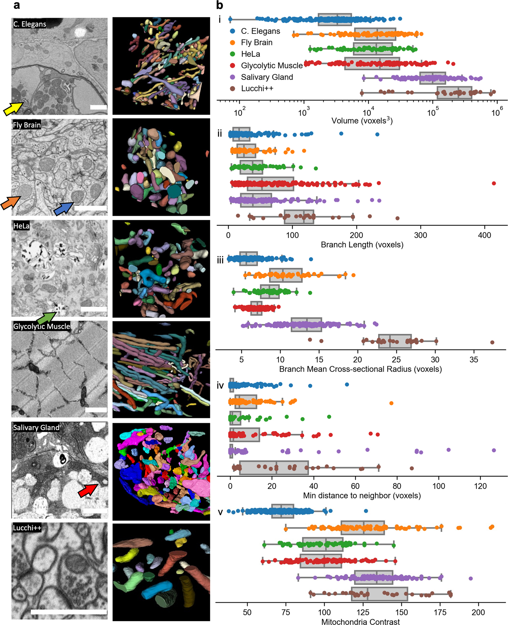
a. 2D representative images (left) and 3D reconstructions (right) for the benchmark test sets. Top to bottom: C. elegans, Fly brain, HeLa cell, Glycolytic muscle, Salivary gland, Lucchi++. Yellow arrow, membranous organelle; orange and blue arrows, lightly and darkly stained mitochondria; green arrow, heavy metal precipitate; red arrow, mitochondrion and tightly apposed salivary granule in the acinus. b. Comparison of individual mitochondria and box plots across benchmarks by (top to bottom): (i) volume (log scale), (ii) branch length, (iii) mean cross-section radius, (iv) minimum distance to neighbor (all in voxels) and (v) mitochondrial contrast. Blue, C. elegans n=241; orange, fly brain n=91; green, HeLa cell n=68; red, glycolytic muscle n=104; purple, salivary gland n=131; brown, Lucchi++ n=33. Scale bar 1 μm.

Similarly, the benchmark volumes encapsulate different mitochondrial morphologies and varying levels of difficulty. We skeletonized and created meshes for all mitochondria to make quantitative comparisons of volume, length and cross-sectional radius along branches in the skeleton, minimum distance between a mitochondrial mesh and its nearest neighbor, and difference between the brightest and darkest voxel in each mitochondrion (Figure 2b, i–v), The simple mitochondria in the fly brain volume have distinct variants: lightly stained with poorly defined cristae and darkly stained with well-defined cristae (Figure 2a, orange and blue arrows respectively). The HeLa cell volume is cluttered with organelles and vesicles and has localized heavy metal precipitates (green arrow). The C. elegans volume has overall lower contrast (Figure 2b, v), as expected for an HPF sample, and presents difficult to segment mitochondrial morphologies – small puncta and skinny tubules (Figure 2b, i–iii). There are also membranous organelles ³⁹ that appear similar to mitochondria with swollen cristae at these resolutions (yellow arrow). The glycolytic muscle volume has a relatively uncluttered background but complex and elaborately branched morphologies. The salivary gland volume is the most challenging because of flat and bowl-shaped mitochondria tightly pressed against salivary granules (red arrow), weak staining, and close packing of the mitochondria themselves (Figure 2b, iv).

Deep learning model and postprocessing

For 2D instance segmentation, we adopted Panoptic-DeepLab ⁴⁰ (PDL). PDL is an encoder-decoder architecture, like the standard U-Net ⁴¹, that takes a bottom-up approach to instance segmentation and scales to segment an arbitrarily large numbers of objects within a field of view (top-down and direct set prediction algorithms like Mask R-CNN ⁴² and Mask2Former ⁴³ cap the number of detections). We trained PDL models to infer mitochondrial semantic segmentations, centers and per-pixel x and y offsets from the associated object’s center (Figure 3a). To create segmentations at resolutions higher than the input image resolution, we employed PointRend ⁴⁴, which iteratively interpolates and reevaluates the label at the most uncertain pixels. This feature allows the model to accept downsampled images and output precise segmentation boundaries at the original resolution without a resolution-specific model architecture (Supplementary Figure 5). The semantic segmentation, offsets, and object centers were postprocessed into an instance segmentation.

Figure 3: Deep learning model and postprocessing pipeline to create 2D or 3D instance segmentations.

a. Schematic of Panoptic-DeepLab showing the input grayscale image (left;, blue boxes, encoder layer outputs; black boxes, ASPP layer outputs; gray boxes, decoder layer output. Outputs of the network are (left to right) semantic segmentation, up-down offsets, left-right offsets, and the instance centers heatmap. Far right, instance segmentation created from the outputs. b. Instance matching across adjacent slices uses intersection-over-union (IoU) and intersection-over-area (IoA) scores. Clockwise from top left: predicted segmentation of slice j, j+1, IoU and IoA merging, IoU only merging. c. Result of median filtering in direction of black arrow d. From left to right: Stacked 2D segmentations of before matching, after forward matching only and after forward and backward matching. Black arrows denote direction of matching. e. An example of 3D instance segmentation of mitochondria after running inference in (left to right) xy, xz, yz directions, and far right, and merging them into a consensus.

To generalize model inference to three dimensions, we tracked 2D instance predictions through a volume EM stack by performing 1-to-1 matching of objects across consecutive slices using the Hungarian algorithm ⁴⁵. We also adopted two postprocessing steps to counter oversplitting errors common for this approach. First, we computed intersection-over-area (IoA) scores for objects that were unmatched because of the 1-to-1 assumption. Unmatched objects with IoA scores over a threshold value were merged to the label of the object with which they overlapped in the preceding slice (Figure 3b). Second, we calculated 2D instance segmentations using median semantic segmentation probabilities over neighborhoods of three or more slices to cover gaps and produce smooth and continuous objects in 3D (Figure 3c). Finally, we performed matching in the reverse direction through the stack to account for branched morphologies (Figure 3d). Optionally, for isotropic-voxel volumes, ortho-plane inference ⁴⁶ can be applied. Here, inference is performed independently on stacks of xy, xz, and yz images and the predictions are combined into a single consensus segmentation using the same algorithm developed for our crowdsourced annotations (Figure 3e). IoA-based merging, median filtering, and ortho-plane inference steps all yielded significant improvements on the volumetric benchmark datasets (Supplementary Table 1).

The particulars of this model architecture and postprocessing scheme were chosen to balance usability and segmentation performance. As we describe later, we can quickly segment large 3D datasets with limited compute resources because only a few 2D image planes are ever held in memory at a time. However, we also experimented with two other methods. The first was a model based on EfficientDet ⁴⁷ that has half the parameters of Panoptic-DeepLab but uses the same prediction task and 2D and 3D postprocessing. The second was a UNet-BC as implemented in PyTorch Connectomics ⁴⁸ and previously developed for the MitoEM benchmark. Briefly, this model predicts two semantic segmentations: one for the bulk of the mitochondrion and another for the outer boundary. These predictions are postprocessed into an instance segmentation using the watershed algorithm applied in 3D.

MitoNet training and evaluation

The encoder network in our experiments was a ResNet50 ⁴⁹ pre-trained on CEM1.5M using the SwAV ⁵⁰ self-supervised learning algorithm (the effect of pre-training is summarized in Supplementary Table 2). Our best performing PDL model, MitoNet, was trained for 120 epochs on CEM-MitoLab. On the benchmark datasets we observed that it segmented a variety of mitochondrial instances accurately in 2D and 3D (Figure 4a, b). MitoNet performed best on the relatively simple brain tissue datasets (fly brain and Lucchi++) with both semantic IoU and F1@75 scores around 0.9 or higher (Figure 4c). Detailed performance metrics are included in Table 1. MitoNet’s F1@75 score of 0.88 on the Lucchi++ test set matched specialist models that were trained exclusively on the Lucchi++ training data ⁵¹. Despite the heterogeneity of the TEM benchmark and that only 16% of CEM-MitoLab was comprised of TEM images, the model reached an average F1@75 score of 0.68 (unlike the other benchmarks F1 was calculated in 2D). While a small subset of images in the TEM benchmark were not well segmented, more than 75% had F1@50 scores greater than 0.6, and the median F1@50 was greater than 0.8 (Supplementary Figure 6b).

Figure 4. MitoNet results on benchmarks.

a. Representative 2D images showing MitoNet segmentation performance; left column shows predictions and right column shows ground truth. Top to bottom: C. elegans, Fly brain, HeLa cell, Glycolytic muscle, Salivary gland, Lucchi++, and TEM benchmarks. b. Representative 3D ground truth and predicted segmentations from MitoNet on the volume EM benchmarks. Red and green, predicted mitochondrial instances, blue and orange, ground truth instances. Black arrow, example of segmentation expected to return a high IoU but low F1 score. c. Left, MitoNet F1 score on each benchmark as a function of IoU threshold; right, IoU scores. d. Left, MitoNet F1 scores on volume EM benchmarks as a function of IoU threshold, after model finetuning on a small fraction of labeled patches; right, IoU scores achieved by the finetuned models. Numbers indicate number of patches used for finetuning e. Left, comparison of mean F1 score for models trained on different datasets plotted against IoU threshold; right, mean IoU scores. All benchmarks except the salivary gland are included in the mean. Crowd., crowdsourced. Scale bar 1 μm.

Table 1.

MitoNet performance on the benchmarks. All metrics are calculated in 3D excluding those for the TEM benchmark. Metrics for the TEM benchmark are averages (N=100). AP, Average Precision, PQ, Panoptic Quality

Datase	IoU	F1@50	F1@75	AP@50	AP@75	PQ
C. Elegans	0.604	0.483	0.325	0.318	0.194	0.376
Fly Brain	0.902	0.940	0.885	0.887	0.794	0.831
HeLa	0.791	0.728	0.503	0.573	0.336	0.571
Glycolytic Muscle	0.840	0.682	0.601	0.518	0.430	0.557
Salivary Gland	0.103	0.036	0.008	0.018	0.004	0.022
Lucchi++	0.871	0.879	0.879	0.784	0.784	0.783
TEM	0.717	0.763	0.682	0.654	0.559	0.670

On the more difficult HeLa and glycolytic muscle benchmarks, MitoNet achieved semantic IoU scores of 0.79 and 0.84, but lower F1@75 scores of 0.5 and 0.6. For the HeLa benchmark, the model successfully ignored much of the cluttered intracellular features, but we did observe several FPs caused by Golgi (data not shown). The IoU and F1 scores on the glycolytic muscle dataset were high given that only a handful of training images were from muscle tissue, and none were from glycolytic muscle (whose mitochondrial ultrastructure is markedly different ³²). Although MitoNet correctly detected 78% of closely apposed mitochondria (i.e., < 5 voxels to nearest neighbor) at an IoU threshold of 0.5 in the HeLa volume and 52% in the glycolytic muscle, visual inspection and the lower instance compared to semantic segmentation scores suggest that identifying individual mitochondria in crowds remains a challenge (Supplementary Figure 6a, min distance plot). Figure 4b shows examples of accurate mitochondrial segmentations, including a heavily branched mitochondrion, as well as overmerging and oversplitting errors that our method was prone to make; such errors could substantially lower F1 scores even when pixel-level accuracy was high (black arrow).

The C. elegans dataset was challenging because of small and low-contrast mitochondria that were tightly packed together. Here, we used a lower vote threshold of only one plane for ortho-plane inference to increase IoU from 0.44 to 0.60 and F1@75 from 0.18 to 0.33 (Supplementary Table 1). MitoNet struggled to detect mitochondria smaller than 1,000 voxels (~ 0.25 μm³); these accounted for about 25% of all FNs (Supplementary Figure 6). The model also performed slightly worse on mitochondria with lower contrast (mean grayscale of TP, 75.9; FN, 70.5, p<0.001; see Supplementary Table 3 for complete statistics). Closely apposed instances accounted for over 75% of all FNs at an IoU threshold of 0.5. The model mostly avoided erroneously labeling the membranous organelles, but occasionally labeled some vesicles as mitochondria (Figure 4a, yellow arrow). On the most challenging benchmark, the salivary gland, MitoNet achieved an IoU score of just 0.10 and F1@50 of 0.04.

Our smaller EfficientDet-based model, MitoNet-mini, had an average IoU score across the benchmarks that was only 4.5% worse than MitoNet while using 66% less GPU memory per image (Supplementary Figure 6c, Supplementary Table 4). There was a sharper decline in average F1@75 score (13.5%) which suggests that the model did not have enough capacity to fit the harder instance segmentation task. On the other hand, the UNet-BC model outperformed MitoNet on both IoU and F1@75 scores by 4.0% and 10.2%, respectively (Supplementary Figure 6c, Supplementary Table 5). However, this came at the cost of nearly 4x more GPU memory per image and, for the largest benchmark dataset of just 1.5 GB, required 28 GB of memory to postprocess.

Although MitoNet can reliably provide automatic segmentations in a variety of contexts, it is possible to improve its performance on a particular dataset via finetuning. For each volume EM benchmark we took a small sample (N) of patches constituting < 2% of all voxels (N=5 for C. Elegans, HeLa, fly brain; N=8 for glycolytic muscle; N=16 for Lucchi; N=64 for salivary gland) and minimally finetuned MitoNet for 100 epochs. Finetuning improved IoU scores by 19.8%, with all but the salivary benchmark exceeding IoUs of 0.8; F1@75 scores improved by 10.4% (Figure 4d, Supplementary Table 6). This underscores an important point: Even when the generalist MitoNet model fails on a dataset, it is still a strong starting point to train a specialist model with a modest number of examples and compute time. A movie describing the procedure of model finetuning with empanada is also included (Supplementary Movie 1).

Finally, we directly probed the efficacy of CEM-MitoLab against other training datasets by measuring the performance of models across all benchmarks except the salivary gland volume. We trained models for approximately 10,000 iterations to account for the different number of images in each dataset (for comparison, the 120 epochs used for MitoNet was equivalent to about 40,000 iterations). The model trained on the Heinrich et al. dataset performed poorly on the benchmarks, likely because of its small size and limited breadth. Training on MitoEM, a large but homogeneous neuronal dataset, gave F1@75 scores of 0.86 and 0.75 on the fly brain and Lucchi++ volumes, but scores of 0.25, 0, 0.07, and 0.01 on the TEM, C. elegans, HeLa cell, and glycolytic muscle benchmarks. The model trained on expert corrected crowdsourced annotations was almost matched by a model trained on our legacy dataset – a 5x larger, reasonably heterogeneous sampling of 19 volumes, over 500 TEM images, and over 2,000 randomly chosen 2D patches from CEM500K. In both cases, IoU and F1 scores were substantially better across all benchmarks than training on MitoEM (Figure 4d, Table 2). Indeed, even training on the uncorrected student consensus annotations was better than training on MitoEM for all benchmarks except the fly brain volume, emphasizing how critical data diversity is, even at the expense of per-instance accuracy (Supplementary File 2). Sparsely sampled, noisy, but heterogeneous labeled data can be more effective for training generalist segmentation models than much larger densely annotated, expert proofread, but homogeneous data. Our best results were achieved by training on CEM-MitoLab (i.e., the combination of legacy and expert proofread crowdsourced annotations).

Table 2.

Average results on all benchmarks (excluding the Salivary Gland) by models pretrained on CEM1.5M and trained on different labeled datasets.

Training Dataset	Mean IoU	Mean F1@50	Mean F1@75	Mean AP@50	Mean AP@75	Mean PQ
Heinrich et al.	0.001	0.001	0.001	0.001	0.000	0.001
MitoEM	0.524	0.425	0.328	0.339	0.266	0.346
Legacy	0.697	0.648	0.504	0.520	0.384	0.530
Crowdsourced	0.667	0.642	0.455	0.523	0.358	0.512
Crowdsourced & Proofread	0.753	0.698	0.542	0.568	0.411	0.566
CEM-MitoLab	0.775	0.737	0.622	0.623	0.504	0.621

Analyzing Mitochondrial Morphologies in Mouse Kidney and Liver Tissue

Mitochondria are enriched in and critical to kidney function especially in proximal tubules, and their dysfunction marks renal disease and injury ^24–26,52. Despite the centrality of mitochondria in renal pathology, existing studies are limited by a reliance on light microscopy, 2D EM, or semantic segmentations of limited volume EM data ^53–55. To demonstrate the power of MitoNet for general mitochondrial instance segmentation, and to generate 3D ultrastructural correlates of known differences in mitochondrial energetics between proximal and distal tubules ⁵⁶ we used the same model to automatically segment tens of thousands of mitochondria in two previously unseen volumes from mouse kidney tissue downloaded from OpenOrganelle ³⁶. The ROIs contained primarily distal tubules and proximal tubules (10 GB each). Additionally, an ROI of hepatocytes from liver tissue (30 GB) were cropped from another volume for comparison. The full python package that we created to run MitoNet inference as well as the postprocessing pipeline is called empanada, while a user-friendly napari plugin of the same name allows easy GUI-based inference and post-processing, point-and-click merge and split operations, and model finetuning (Supplementary Movie 2). MitoNet segmented 7,718, 15,180, and 61,244 objects in each ROI, respectively. On a system with a single GPU and just 16 GB of RAM, automatic segmentation of all objects with empanada took 1.5 hours for each of the kidney volumes and 3.5 hours for the liver volume (watershed postprocessing, like that used for UNet-BC, required 512 GB of RAM). Out-of-the-box, MitoNet predictions were immediately useful for visualizing the data and identifying dramatically different mitochondrial morphologies. 2D slice and full 3D instance segmentations of mitochondria from full ROIs are shown in Figure 5a, while mitochondria from individual cells, and representative instances of mitochondria showing dramatic variation in morphologies, is shown in Figure 5b. Mitochondria in both kidney volumes were densely packed into rows, polarized towards basolateral surfaces, and were revealed to have flattened morphologies. Some 6% of mitochondria in the proximal tubule (middle row) were fused into large and complex networks in sharp contrast to the much less branched morphologies in the distal tubule. Thus, with automatic MitoNet segmentation, limited morphological assessments from light microscopy imaging of proximal tubules ⁵⁴ can now be extended and quantified at an individual organelle level with the resolution of volume EM. Mitochondria in the hepatocytes appeared to be relatively simple tubes and spheroids in line with previous analyses ^57–60; however, many instances were visible with long and skinny protrusions – possibly nanotunnels ⁶¹ – extending into the surrounding cytoplasm. As further evidence of the model’s ability to generalize, we observed accurate segmentations of mitochondria in endothelial cells incidentally captured within the volumes as well (Supplementary Movie 1).

Figure 5. MitoNet results on volumes of mouse liver and kidney.

a. Rows from top to bottom correspond to kidney distal tubule, kidney proximal tubule, and liver. Left column shows representative 2D images of MitoNet segmentation (scale bar, 5 μm); right column shows 3D predictions on the entire volume (small and boundary objects removed). b. Left column shows a zoomed in ROI of raw model predictions (basolateral surfaces of cells on top); right column shows representative mitochondrial models after manual cleanup. c. Plot of the fraction and type of cleanup operation required for a randomly chosen sample of model-predicted instances from kidney distal (n=347), kidney proximal (n=256) and liver (n=319) tissue. d. Plot of distance to the nearest basolateral surface, in microns, for randomly sampled mitochondria from kidney distal (blue) and kidney proximal (red) volumes after cleanup. e. Box plot comparisons of mitochondrial volume, surface area, cross-sectional radius, elongation, and flatness across the three volumes after cleanup (outliers not shown). Blue, kidney distal (n=405 for d and e), green, kidney proximal (n=250), orange, liver (n=321).

Notably, 89%, 80%, and 60% of randomly sampled instances from the hepatocyte, distal tubule, and proximal tubule volumes, respectively, required no edits. In line with our results on the benchmarks, MitoNet predictions rarely required per-pixel corrections, but merge and split errors occurred in a data-specific manner (Figure 5c). For example, 12% of sampled distal tubule instances required splitting, while 21% in the proximal tubules needed merging – multiple merge operations were often required for complex mitochondria. With empanada’s point-and-click proofreading operations we took under 2 hours to split and merge all the sampled distal tubule instances. Proofread instance segmentations can be used for a variety of quantitative analyses. We assessed mitochondrial polarization by measuring the distribution of their distances from basolateral surfaces in distal and proximal tubules (Figure 5d) and discovered statistically significant differences (median distance in distal tubule, 3.38 μm; proximal tubule, 0.86 μm, p<0.001). Additionally, other simple measurements accessible only with instance segmentation, e.g., volume, surface area, cross-sectional radius, elongation, and flatness, also showed intriguing differences between these groups (Figure 5d, statistical measures summarized in Supplementary Table 7). Such large-scale observations of mitochondrial architectures in 3D and at high resolutions may reveal new and unexpected insights in kidney and other tissue pathologies.

Discussion

In this paper we have reported several resources for the growing volume EM community: a massive and heterogeneous unlabeled cellular EM image dataset that samples over 2 PB of EM data (CEM1.5M), a similarly heterogeneous dataset of >135,000 instances of labeled mitochondria (CEM-MitoLab), a model trained on this dataset (MitoNet), a set of diverse of 2D and 3D benchmarks (MitoNet Benchmarks) for model testing, and a Python package and napari plugin (empanada) for immediate use of MitoNet with proofreading tools. We also describe these datasets with a simple spreadsheet implementation of REMBI ⁶² containing image and biological metadata. Together, these resources relieve the “segmentation bottleneck”, a current constraint in volume EM workflows otherwise replete with technological and application advances. We note that CEM1.5M and empanada can be used for other features in cellular EM, and while CEM-MitoLab, MitoNet and benchmarks are mitochondria specific resources, their performance validates the strategy of broad but shallow sampling of cellular contexts to create general segmentation models for any organelle. Heterogeneity of training data is crucial, as shown by the result that models trained on our noisy crowdsourced annotations generalize better than models trained on narrow but expertly labeled data like MitoEM. Expert proofreading was still necessary to achieve our best results, so broader expert participation in future shared efforts could greatly benefit the field. Similarly, homogeneous volume EM benchmarks derived from connectomics data are poor tests of generalization; the Lucchi++ benchmark has been mined to the point of performance saturation ^51,63. The assortment of mitochondria, contexts, quality, and overall difficulty in our benchmarks offer a stiff test for new models, but future benchmarks must be continually expanded to avoid exhaustion.

We made an important decision to forego 3D approaches. This allowed us to leverage abundant 2D datasets to represent a much broader range of cells and tissues, and also maximized images sampled – our crowdsourced dataset of ~6,000 2D labeled images would have equated to just 30 3D labeled images of comparable dimensions. Staying in the 2D regime keeps hardware requirements low as well, congruent with our belief that true democratization demands that tools be usable without DL expertise or expensive compute resources – although we note that our workflows work both on consumer-grade laptops with no GPUs and on HPCs with many. The methods we developed in this work, such as median filtering and ortho-plane inference, retain the efficiencies of labeling and running model inference in 2D but utilize 3D context where possible. As shown by our results with the UNet-BC model, postprocessing with full 3D context can improve instance segmentation at the cost of usability. We expect native 3D model architectures to surpass our methods eventually. Even then, empanada can be used to quickly segment and proofread the 3D data needed to train such models.

True human-level mitochondrial instance segmentation on any 2D or 3D EM image may be possible. Better methods are needed to segment small and closely packed instances, and unusual cellular contexts or low contrast and resolution images pose some difficulties. That said, semantic segmentations were consistently accurate on most datasets tested, and a proof-of-principle experiment on kidney and liver volumes shows that MitoNet is already a powerful and accessible tool for rapid visualization and accurate quantification of mitochondrial morphologies, even without proofreading for some datasets (Supplementary Table 7). Current DL pipelines using specialist models rely on repeated cycles of human-in-the-loop annotation, training, inference, and proofreading. With generalist DL segmentation models, like MitoNet for mitochondria, this cycle is reduced to just inference and proofreading on any EM dataset. Even for datasets where out-of-the-box inference is poor, our napari plugin, empanada, enables quick finetuning on sparsely sampled 2D patches for improved results. Future expansions of the CEM resources will further enable model generality irrespective of feature segmented; such models, whether for semantic, instance, or panoptic segmentation, can be trained using empanada and broadly shared for deployment.

Volume EM is catalyzing a “quiet revolution” ⁶⁴ by enabling large-volume high-resolution 3D images of cellular and subcellular features, revealing insights into connectomics and cell biology. Accurate and efficient extraction of features of interest from these massive ultrastructural images lends itself to computational solutions. Here we create large-scale and relevant training data resources and train a generalist model to segment mitochondria in any EM image. We also release an easy-to-use software plugin for users to deploy this model on their own data and execute downstream “clean up” steps to generate polished mitochondrial segmentations. In tandem with recent initiatives to generate and share large volume EM reconstructions ³⁶, our methods provide a blueprint for future applications, thereby expanding the segmentation toolkit and helping accelerate discoveries in this exciting field.

$$w_i=\frac{{n_i}^{-\gamma }}{{\sum }_{j=1}^N{w}_j}$$

STAR Methods

Resource Availability

Lead Contact:

Further information and requests for resources should be directed to Kedar Narayan (narayank@mail.nih.gov)

Materials Availability:

This study did not generate new materials.

Data and Code Availability

Datasets have been deposited at EMPIAR and are publicly available as of the date of publication: CEM1.5M (https://www.ebi.ac.uk/empiar/EMPIAR-11035/), CEM-MitoLab (https://www.ebi.ac.uk/empiar/EMPIAR-11037/), MitoNet Benchmarks (https://www.ebi.ac.uk/empiar/EMPIAR-10982/).

Code for the empanada library is available at 10.5281/zenodo.7373985. Code for the empanada-napari plugin is available at 10.5281/zenodo.7374004. Pre-trained models are available on Zenodo: CEM1.5M weights (https://zenodo.org/record/6453160#.YnPjEy-cbTR), MitoNet (https://zenodo.org/record/6327742#.YnLciy-cbTS).

Any additional information required to reanalyze the data reported in this paper is available from the lead contact upon request.

Method Details

CEM1.5M Creation

The expansion of CEM500K to create the CEM1.5M dataset followed the data standardization and curation protocols presented in our previous work ³⁵. External datasets were either downloaded in their entirety or, for large datasets stored online in next generation file formats (n5 or zarr), accessed either with the CloudVolume or fibsem-tools APIs. Datasets larger than 5 GB were randomly cropped into 320 cubes of 256³. Metadata and proper attribution for each dataset is available in Supplementary file 1. TEM and STEM images were grouped into directories based on imaging project or publication before processing. 3,000 NCI TEM images with magnifications between 1000x (~16 nm pixel) and 3000x (~6 nm pixel) and excluding negative stain and immunogold label images were randomly selected from a library of over 2×10⁵ images. Metadata for these images was unavailable.

Crowdsourced Annotation

Our Zooniverse workflow closely approximated the Etch-a-cell project ¹³. Flipbooks of image patches from 3D data (8-bit tif stacks of five consecutive images of 224×224) were contrast rescaled to 25–235 and interpolated to 480×480 for easier viewing. For 2D images contrast was similarly rescale but crops of 512×512 were used. Over the course of the project, the Zooniverse chat channel and a formal instruction session were used to review examples and explain errors. During expert proofreading, the correction of FP and FN detections was emphasized over pixel-level painting; disagreements were discussed and resolved as a group. All annotations were passed through a connected components filter after proofreading.

The input to the consensus algorithm was a set of N annotations (the retirement limit) containing K mitochondrial detections (Supplementary Figure 3 i). An undirected graph was initialized where each node corresponded to one of the K detections. Edges were added to the graph to connect detections with mask IoU scores that exceeded a small threshold value of 0.1 (the same algorithm, when applied during ortho-plane inference, used a threshold of 0.01). Each connected component in the detection graph was then processed independently. Nodes in a connected component were organized into cliques where all detections within a clique shared edges with IoU scores greater than 0.75 (Supplementary Figure 3 ii,iii). Edges between detections in different cliques were retained. An iterative algorithm was applied to determine whether cliques should be merged or remain split. First, the most connected clique (i.e., the one with the most edges; node C in Supplementary Figure 3 ii,iv; A in 3 iii,v) was selected. Second, if any of the most connected clique’s neighbors contained more detections, then the most connected clique was dissolved and its detections were pushed out to each of its neighbors (C in Supplementary Figure 3 iv). Otherwise, all the most connected clique’s neighbors were dissolved and their detections were merged into the most connected clique (B and D in Supplementary Figure 3 iv, B and C into A in 3 v). These two steps were repeated until no edges were left between cliques. Each clique represented an object instance. The detection masks within a clique were added together to form an image where each pixel had a value from 1 to N. A vote threshold was applied to create the final binary instance mask. All instances were combined into the final consensus annotation (Supplementary Figure 3 vi).

Labeled and benchmark dataset creation

The “legacy” portion of CEM-MitoLab came from publicly available mitochondrial segmentations (Kasthuri++, Guay, UroCell, MitoEM, Heinrich et al. and Perez et al.) ^37,65,66 and previous in-house segmentation projects. Of these, MitoEM already had instance labels, and a connected components filter was applied to convert other semantic labels to instance segmentations. All in-house segmentation projects were proofread or annotated by experienced researchers. The projects included annotations of whole volumes, TEM images, and a random selection of patches from CEM500K ³⁵; none were derived from the benchmark datasets. For volumes and TEM images, 512×512 crops were taken from xy planes, or all three planes for isotropic volumes, and passed through the deduplication and filtering pipeline to remove redundant and uninformative patches. Legacy images were used as-is except for MitoEM-H and MitoEM-R volumes which were binned to 16 nm pixels and Heinrich et al. images which were downloaded at 8 nm resolution. To create the alternative training datasets in Figure 4, MitoEM and Heinrich et al. ground truth ROIs were sliced to 2D images. For MitoEM, patches of size 512×512 were cropped from xy planes only. The Heinrich et al. volumes were cropped into patches of 224×224 or smaller from xy, xz and yz planes, and 2D segmentations were passed through a connected components filter.

The HeLa cell, C. elegans, fly brain and salivary gland benchmark datasets were annotated by ariadne (https://ariadne.ai/). The glycolytic muscle ³² dataset was annotated in-house. The benchmark derived from Lucchi++ was generated by applying a connected components filter to the binary mitochondrial labelmaps followed by manual proofreading. To be rigorous, we excluded from CEM1.5M and CEM-MitoLab not just the benchmark datasets, but also images related to them, e.g., the entire Lucchi++ training dataset, all other drosophila neuronal data from OpenOrganelle, and FIB-SEM and STEM data from the in-house C. elegans project.

Images in the TEM benchmark were gathered from internal NCI TEM repositories, the Cell Image Library (http://www.cellimagelibrary.org/home), Nanotomy (http://www.nanotomy.org/), and the WormImage Database (https://www.wormimage.org/), and metadata included where possible. To match the TEM pixel sizes sampled in the CEM-MitoLab dataset, images were minimally downsampled such that none had pixels smaller than 6 nm. Ground truth segmentations were created manually by two experienced researchers.

CEM1.5M Pre-training

Unsupervised pre-training used the SwAV algorithm ⁵⁰. A ResNet50 ⁴⁹ model was trained for 200 epochs with a batch size of 256; other hyperparameters used defaults defined in https://github.com/facebookresearch/swav. Image augmentations included 360-degree rotations, randomly resized crops, brightness and contrast jitter, random Gaussian blur and noise, and horizontal and vertical flips. To correct for the imbalance in the number of patches per dataset, weighted random sampling was applied. Weights per dataset were calculated by:

$$w_i=\frac{{n_i}^{-\gamma }}{{\sum }_{j=1}^N{w}_j}$$

γ was a float from 0 to 1, n_i was the number of patches from the i^th dataset, and N was the total number of datasets. We used γ=0.5.

MitoNet model architecture, training parameters, and post-processing

MitoNet was based on Panoptic-DeepLab (PDL). PDL is an encoder-decoder style network that uses atrous spatial pyramid pooling (ASPP) to integrate features over multiple scales; our configuration included one ASPP decoder for semantic segmentation prediction and another for instance center and offsets prediction. A ResNet50, pre-trained as detailed above, was used as the encoder network. To preserve spatial information, strides in the last downsampling layer were replaced with dilation such that the output from the encoder was 16x smaller than the input. Dilation rates in the ASPP modules were set to 2, 4, and 6 with 256 channels per convolution and dropout probability of 0.5. The semantic and instance decoders had a single level at which the output from the first layer in the encoder was fused to the interpolated ASPP output via depthwise separable convolution. Convolutions had 32 channels in the semantic decoder and 16 in the instance decoder. The semantic segmentation, instance center and offset heads used a single depthwise separable convolution with kernel size of 5. The PointRend ⁴⁴ module was added to refine the semantic segmentation. Module parameters used the defaults defined in Detectron2 ⁶⁷. Briefly, during training, the segmentation logits were upsampled by a factor of 4 to the original image resolution and then refined in a single step. During evaluation, two refinement steps were applied with the segmentation logits being upsampled by a factor of 2 at each step. An arbitrary number of interpolation and refinement steps can be applied sequentially to upsample the segmentation to a desired resolution. The overall loss function was:

$${\text{L}}_{\text{total}}={\text{L}}_{\text{sem}}+\mathrm{\alpha }{\text{L}}_{\text{center}}+\mathrm{\beta }{\text{L}}_{\text{offset}}+\gamma {\text{L}}_{\text{pointrend}}$$

α, β, γ were constants set to 200, 0.01 and 1, respectively. L_sem was the semantic segmentation loss computed as the bootstrapped (binary) cross-entropy where only the top 20% of cross-entropy values were averaged across a batch. L_center was the instance center regression loss and L_offset was the center offset loss calculated as mean squared error and absolute error (L1), respectively. L_pointrend was the PointRend loss calculated as the (binary) cross-entropy.

The only difference in architecture between MitoNet and the MitoNet-mini model was the replacement of ASPP modules with BiFPN modules ⁴⁷. Both the semantic and instance decoders were replaced with a stack of three BiFPN modules each with a feature dimension of 128. The model architecture and loss function were otherwise the same.

MitoNet and MitoNet-mini were trained on CEM-MitoLab using the One Cycle learning rate policy ⁶⁸ with AdamW ⁶⁹ for 120 epochs. The max learning rate was set to 0.003 for MitoNet and 0.001 for MitoNet-mini with weight decay of 0.1 and momentum cycled from 0.85 to 0.95. Learning rate warmup lasted for the first 30% of training epochs. The batch size was 64. Image augmentations included large scale jitter ⁷⁰, random cropping of a 256×256 patch, 360-degree rotations, brightness and contrast adjustments, and vertical and horizontal flips. Weighted sampling, as defined above for CEM1.5, used γ=0.3. Postprocessing of the model outputs in an instance segmentation used the method developed for Panoptic-DeepLab. In all experiments, the non-maximum suppression kernel size was set to 7 and the center confidence threshold was set to 0.1.

Unet-BC model architecture, training parameters, and post-processing

For the Unet-BC model we used the implementation provided in PyTorch Connectomics ⁴⁸. The model was trained to predict one semantic segmentation for mitochondria and another for mitochondrial contours (i.e., boundaries between mitochondria and background). The only change made to the default model configuration was a doubling of the number of filters in each layer. The overall loss function was:

$${\mathrm{L}}_{\text{total}}={\text{L}}_{\text{sem}}+{\text{L}}_{\text{boundary}}+\alpha ({\text{L}}_{\text{sem\_dice}}+{\text{L}}_{\text{boundary\_dice}})$$

α was a constant value of 0.5. L_sem and L_boundary were the binary cross-entropy losses calculated for the semantic and boundary segmentations respectively. L_{sem_dice} and L_{boundary_dice} were the dice losses ⁷¹ calculated for the semantic and boundary segmentations respectively. The training protocol was identical to that used for MitoNet, CEM1.5M pre-trained weights could not be used to initialize any Unet-BC models because the encoder used was not a ResNet50.

To postprocess the model outputs into an instance segmentation, the semantic segmentation and boundary predictions were binarized over a threshold. Boundaries were then subtracted from the semantic segmentation before labeling connected components. The watershed algorithm, using the connected components as markers, was then applied in 2D or 3D in order to label the pixels or voxels in the boundary prediction.

Benchmark inference and evaluation

For the MitoNet and MitoNet-mini models, ortho-plane inference ⁴⁶ was used on all benchmark volumes. During inference over each plane, median semantic segmentation probabilities were calculated from a queue of a few consecutive slices. A queue length of 3 was used for the C. elegans and fly brain, 5 for the HeLa and glycolytic muscle and 7 for the Lucchi++ and salivary gland. Queue lengths roughly track inversely with voxel size. Median probabilities were hardened at a confidence threshold of 0.3 and Panoptic-DeepLab postprocessing was performed. The resultant instance segmentations were passed through a connected components filter. After forward and backward instance matching with IoU and IoA threshold of 0.25, a size and bounding box extent filter were applied to eliminate likely false positives. Minimum sizes were 500 voxels for C. Elegans and fly brain; 800 for HeLa; 1,000 for salivary gland; 3,000 for glycolytic muscle; 5,000 for Lucchi++. Minimum bounding box extent was fixed at eight voxels. The same consensus segmentation algorithm as above was applied to ensemble the three segmentation stacks created by ortho-plane inference. A clique IoU threshold of 0.75 and a vote threshold of 2 out of 3 was used for all benchmarks except the C. elegans and salivary gland volumes. For those a vote threshold of 1 out of 3 was used. This was in response to the relatively low IoU scores observed. While a vote threshold of 1 was used, each clique was required to have at least 2 detections; this enabled increases in IoU score without the introduction of many FPs. The consensus algorithm occasionally produced overlapping instances. Instances overlapping more than 100 voxels were merged; otherwise, the few overlapping voxels would be assigned to whichever instance was processed last.

For the Unet-BC model, ortho-plane inference was used on all benchmark volumes. First, semantic and boundary segmentation probabilities from xy, xz, and yz stacks were averaged together in 3D and binarized at thresholds of 0.3 and 0.2, respectively. Next, the boundary segmentation was subtracted from the semantic segmentation before labeling connected components. Finally, connected components larger than a minimum size were used as markers for the watershed algorithm. Minimum sizes for each volume were the same as those used for MitoNet postprocessing detailed above.

MitoNet finetuning

Finetuning was performed by manually selecting ground truth labeled patches of size 256² pixels from each of the six volume EM benchmarks. The number of patches used per volume were five for C. Elegans, fly brain, and HeLa cell (~2% of all voxels); eight for the glycolytic muscle (~0.5%); 16 for Lucchi++ (~0.8%); and 64 for salivary gland (~0.3%). The same hyperparameters used for MitoNet training were also used for finetuning with the exception that the max learning rate was set to 0.001 and the batch size was 16. All finetuned models were trained for 100 epochs.

OpenOrganelle volume inference and analysis

For the “Mouse kidney” dataset, two ROIs containing cells in the proximal tubule and distal tubule exclusively (some endothelial cells could not be avoided) were manually chosen from the 128nm overview to download the desired data at 16nm resolution. One ROI from the “Mouse liver” dataset was similarly selected. Inference used the best version of the MitoNet model and was run only on slices from the xy plane with a segmentation confidence threshold of 0.3 and median filter size of 5. A single compute node with a P100 GPU and 16 GB of memory was used. Image volumes and predicted mitochondrial instances were downsampled to 32nm pixel size for visualization and cleanup and a size threshold of 1,000 voxels was applied. For cleanup and quantification, 400 instances were randomly chosen such that they did not touch the boundary and each bounding box was at least 15 pixels long on a side. The empanada napari plugin was used to proofread each instance and merge, split, paint, and erase as required. FPs, mitochondria in endothelial cells, and instances on the boundary after merging were removed. Volume, surface area, flatness and elongation measurements for individual mitochondria were calculated using the LabelShapeStatistics filter implemented in ITK ⁷². Branch lengths and cross-sectional diameters were calculated by first skeletonizing each mitochondrion and computing its distance transform. Lengths were simply the number of voxels in each branch, and the mean cross-sectional diameter was the average of distance transform values that overlapped with the skeleton. Branches shorter than 60 nm were pruned. Mitochondria contrast was calculated as the difference between maximum and minimum intensity voxels in each instance. Basolateral surfaces were approximated by fitting a triangular mesh to manually placed periodic fiducials using the ball pivoting algorithm ⁷³ and the minimum distances between vertices of each mitochondrial mesh to the nearest basolateral surface were calculated.

Quantification and statistical analysis

Sample sizes and statistical tests used are reported in figure and table legends. The decision to use a parametric or non-parametric statistical test was made based on the observed normality of measured quantities. The threshold for statistical significance was 0.05.

Additional Resources

Links and additional explanation of all resources presented in this work are available on our project webpage https://volume-em.github.io/empanada.

Supplementary Material

1

Supplementary File 1. Spreadsheet of available metadata of in-house and externally sourced datasets contributing to CEM1.5M.

2

Supplementary File 2. Model performance scores, when trained by various labeled datasets, for individual benchmarks. The average of these benchmark scores is shown in Fig 4d. Salivary Gland benchmark required finetuning and was not included.

3

Supplementary Movie 1. Finetuning model predictions in empanada-napari. The user picks predetermined or random patches from initial predictions on a given dataset, then runs model finetuning followed by inference on the original dataset.

4

Supplementary Movie 2. Mitochondrial instance predictions by MitoNet, in liver, kidney distal tubule and kidney proximal tubule volumes. 2D predictions in volume EM stacks and 3D reconstructions are shown (with small objects and objects on boundaries removed), as well as examples of highly complex mitochondrial instances.

KEY RESOURCES TABLE.

REAGENT or RESOURCE	SOURCE	IDENTIFIER
Antibodies
Bacterial and virus strains
Biological samples
Chemicals, peptides, and recombinant proteins
Critical commercial assays
Deposited data
CEM1.5M	This paper	10.6019/EMPIAR-11035
CEM-MitoLab	This paper	10.6019/EMPIAR-11037
Benchmark datasets	This paper	10.6019/EMPIAR-10982
Heinrich et al.	Heinrich et al.	https://open.quiltdata.com/b/janelia-cosem-publications/tree/heinrich-2021a/ (no DOI available)
MitoEM	Wei et al.	https://mitoem.grand-challenge.org/MitoEM/ (no DOI available)
OpenOrganelle mouse liver	OpenOrganelle	10.25378/janelia.16913047.v1
OpenOrganelle mouse kidney	OpenOrganelle	10.25378/janelia.16913035.v1
DeepContact Training Data	Liu, L. et al.	10.6084/m9.figshare.19898404.v3
Experimental models: Cell lines
Experimental models: Organisms/strains
Oligonucleotides
Recombinant DNA
Software and algorithms
empanada	This paper	10.5281/zenodo.7373984
empanada-napari	This paper	10.5281/zenodo.7374003
napari	napari contributors	doi:10.5281/zenodo.3555620
arivis Vision4D	Zeiss	Vision4D
Other

Highlights.

• A curated dataset of ~1.5 million diverse unlabeled electron microscopy images

• ~135K segmented mitochondria from existing datasets and crowdsourced annotations

• MitoNet, a deep learning model, accurately segments mitochondria in various contexts

• Empanada, a Python library and napari plugin, allows MitoNet inference and clean-up

References

- 1.Peddie CJ, and Collinson LM (2014). Exploring the third dimension: Volume electron microscopy comes of age. Micron 61, 9–19. 10.1016/J.MICRON.2014.01.009. [DOI] [PubMed] [Google Scholar]
- 2.Titze B, and Genoud C (2016). Volume scanning electron microscopy for imaging biological ultrastructure. Biol. Cell 108, 307–323. 10.1111/BOC.201600024. [DOI] [PubMed] [Google Scholar]
- 3.Scheffer LK, Xu CS, Januszewski M, Lu Z, Takemura SY, Hayworth KJ, Huang GB, Shinomiya K, Maitin-Shepard J, Berg S, et al. (2020). A connectome and analysis of the adult drosophila central brain. Elife 9, 1–74. 10.7554/ELIFE.57443. [DOI] [PMC free article] [PubMed] [Google Scholar]
- 4.Turner NL, Macrina T, Bae JA, Yang R, Wilson AM, Schneider-Mizell C, Lee K, Lu R, Wu J, Bodor AL, et al. (2022). Reconstruction of neocortex: Organelles, compartments, cells, circuits, and activity. Cell 0, 17. 10.1016/J.CELL.2022.01.023. [DOI] [PMC free article] [PubMed] [Google Scholar]
- 5.Yin W, Brittain D, Borseth J, Scott ME, Williams D, Perkins J, Own CS, Murfitt M, Torres RM, Kapner D, et al. (2020). A petascale automated imaging pipeline for mapping neuronal circuits with high-throughput transmission electron microscopy. Nat. Commun. 2020 111 11, 1–12. 10.1038/s41467-020-18659-3. [DOI] [PMC free article] [PubMed] [Google Scholar]
- 6.Januszewski M, Kornfeld J, Li PH, Pope A, Blakely T, Lindsey L, Maitin-Shepard J, Tyka M, Denk W, and Jain V (2018). High-precision automated reconstruction of neurons with flood-filling networks. Nat. Methods 15, 605–610. 10.1038/s41592-018-0049-4. [DOI] [PubMed] [Google Scholar]
- 7.Berning M, Boergens KM, and Helmstaedter M (2015). SegEM: Efficient Image Analysis for High-Resolution Connectomics. Neuron 87, 1193–1206. 10.1016/j.neuron.2015.09.003. [DOI] [PubMed] [Google Scholar]
- 8.Dorkenwald S, Schubert PJ, Killinger MF, Urban G, Mikula S, Svara F, and Kornfeld J (2017). Automated synaptic connectivity inference for volume electron microscopy. Nat. Methods 2017 144 14, 435–442. 10.1038/nmeth.4206. [DOI] [PubMed] [Google Scholar]
- 9.Funke J, Tschopp F, Grisaitis W, Sheridan A, Singh C, Saalfeld S, and Turaga SC (2019). Large Scale Image Segmentation with Structured Loss Based Deep Learning for Connectome Reconstruction. IEEE Trans. Pattern Anal. Mach. Intell. 41, 1669–1680. 10.1109/TPAMI.2018.2835450. [DOI] [PubMed] [Google Scholar]
- 10.Heinrich L, Bennett D, Ackerman D, Park W, Bogovic J, Eckstein N, Petruncio A, Clements J, Pang S, Xu CS, et al. (2021). Whole-cell organelle segmentation in volume electron microscopy. Nat. 2021 5997883 599, 141–146. 10.1038/s41586-021-03977-3. [DOI] [PubMed] [Google Scholar]
- 11.Žerovnik Mekuč M, Bohak C, Hudoklin S, Kim BH, Romih R, Kim MY, and Marolt M (2020). Automatic segmentation of mitochondria and endolysosomes in volumetric electron microscopy data. Comput. Biol. Med. 119, 103693. 10.1016/j.compbiomed.2020.103693. [DOI] [PubMed] [Google Scholar]
- 12.Liu J, Li L, Yang Y, Hong B, Chen X, Xie Q, and Han H (2020). Automatic Reconstruction of Mitochondria and Endoplasmic Reticulum in Electron Microscopy Volumes by Deep Learning. Front. Neurosci. 14, 599. 10.3389/FNINS.2020.00599/BIBTEX. [DOI] [PMC free article] [PubMed] [Google Scholar]
- 13.Spiers H, Songhurst H, Nightingale L, de Folter J, Hutchings R, Peddie CJ, Weston A, Strange A, Hindmarsh S, Lintott C, et al. (2021). Deep learning for automatic segmentation of the nuclear envelope in electron microscopy data, trained with volunteer segmentations. Traffic 22, 240–253. 10.1111/TRA.12789. [DOI] [PubMed] [Google Scholar]
- 14.Guay MD, Emam ZAS, Anderson AB, Aronova MA, Pokrovskaya ID, Storrie B, and Leapman RD (2021). Dense cellular segmentation for EM using 2D–3D neural network ensembles. Sci. Reports 2021 111 11, 1–11. 10.1038/s41598-021-81590-0. [DOI] [PMC free article] [PubMed] [Google Scholar]
- 15.Wei D, Lin Z, Franco-Barranco D, Wendt N, Liu X, Yin W, Huang X, Gupta A, Jang WD, Wang X, et al. (2020). MitoEM Dataset: Large-scale 3D Mitochondria Instance Segmentation from EM Images. Med. Image Comput. Comput. Assist. Interv. 12265, 66. 10.1007/978-3-030-59722-1_7. [DOI] [PMC free article] [PubMed] [Google Scholar]
- 16.Müller A, Schmidt D, Xu CS, Pang S, D’Costa JV, Kretschmar S, Münster C, Kurth T, Jug F, Weigert M, et al. (2021). 3D FIB-SEM reconstruction of microtubule–organelle interaction in whole primary mouse β cells. J. Cell Biol. 220. 10.1083/JCB.202010039. [DOI] [PMC free article] [PubMed] [Google Scholar]
- 17.Buhmann J, Sheridan A, Malin-Mayor C, Schlegel P, Gerhard S, Kazimiers T, Krause R, Nguyen TM, Heinrich L, Lee WCA, et al. (2021). Automatic detection of synaptic partners in a whole-brain Drosophila electron microscopy data set. Nat. Methods 2021 187 18, 771–774. 10.1038/s41592-021-01183-7. [DOI] [PMC free article] [PubMed] [Google Scholar]
- 18.Meyer JN, Leuthner TC, and Luz AL (2017). Mitochondrial fusion, fission, and mitochondrial toxicity. Toxicology 391, 42–53. 10.1016/j.tox.2017.07.019. [DOI] [PMC free article] [PubMed] [Google Scholar]
- 19.Zhang L, Trushin S, Christensen TA, Bachmeier BV, Gateno B, Schroeder A, Yao J, Itoh K, Sesaki H, Poon WW, et al. (2016). Altered brain energetics induces mitochondrial fission arrest in Alzheimer’s Disease. Sci. Rep. 6, 1–12. 10.1038/srep18725. [DOI] [PMC free article] [PubMed] [Google Scholar]
- 20.Pernas L, and Scorrano L (2016). Mito-Morphosis: Mitochondrial Fusion, Fission, and Cristae Remodeling as Key Mediators of Cellular Function. Annu. Rev. Physiol. 78, 505–531. 10.1146/annurev-physiol-021115-105011. [DOI] [PubMed] [Google Scholar]
- 21.Delgado T, Petralia RS, Freeman DW, Sedlacek M, Wang YX, Brenowitz SD, Sheu SH, W Gu J, Kapogiannis D, Mattson MP, et al. (2019). Comparing 3D ultrastructure of presynaptic and postsynaptic mitochondria. Biol. Open 8. 10.1242/bio.044834. [DOI] [PMC free article] [PubMed] [Google Scholar]
- 22.Glancy B, Kim Y, Katti P, and Willingham TB (2020). The Functional Impact of Mitochondrial Structure Across Subcellular Scales. Front. Physiol. 11, 1462. 10.3389/fphys.2020.541040. [DOI] [PMC free article] [PubMed] [Google Scholar]
- 23.Nunnari J, and Suomalainen A (2012). Mitochondria: In Sickness and in Health. Cell 148, 1145–1159. 10.1016/J.CELL.2012.02.035. [DOI] [PMC free article] [PubMed] [Google Scholar]
- 24.Bhargava P, and Schnellmann RG (2017). Mitochondrial energetics in the kidney. Nat. Rev. Nephrol. 13, 629–646. 10.1038/NRNEPH.2017.107. [DOI] [PMC free article] [PubMed] [Google Scholar]
- 25.Doke T, and Susztak K (2022). The multifaceted role of kidney tubule mitochondrial dysfunction in kidney disease development. Trends Cell Biol. 10.1016/J.TCB.2022.03.012. [DOI] [PMC free article] [PubMed] [Google Scholar]
- 26.Emma F, Montini G, Parikh SM, and Salviati L (2016). Mitochondrial dysfunction in inherited renal disease and acute kidney injury. Nat. Rev. Nephrol. 12, 267–280. 10.1038/NRNEPH.2015.214. [DOI] [PMC free article] [PubMed] [Google Scholar]
- 27.Leonard AP, Cameron RB, Speiser JL, Wolf BJ, Peterson YK, Schnellmann RG, Beeson CC, and Rohrer B (2015). Quantitative analysis of mitochondrial morphology and membrane potential in living cells using high-content imaging, machine learning, and morphological binning. Biochim. Biophys. Acta - Mol. Cell Res 1853, 348–360. 10.1016/j.bbamcr.2014.11.002. [DOI] [PMC free article] [PubMed] [Google Scholar]
- 28.Nikolaisen J, Nilsson LIH, Pettersen IKN, Willems PHGM, Lorens JB, Koopman WJH, and Tronstad KJ (2014). Automated Quantification and Integrative Analysis of 2D and 3D Mitochondrial Shape and Network Properties. PLoS One 9, e101365. 10.1371/journal.pone.0101365. [DOI] [PMC free article] [PubMed] [Google Scholar]
- 29.Talwar A, Lin Z, Wei D, Wu Y, Zheng B, Zhao J, Jang WD, Wang X, Lichtman J, and Pfister H (2020). A topological nomenclature for 3D shape analysis in connectomics. In IEEE Computer Society Conference on Computer Vision and Pattern Recognition Workshops, pp. 4245–4253. [Google Scholar]
- 30.Miyazono Y, Hirashima S, Ishihara N, Kusukawa J, Nakamura K-I, and Ohta K (2018). Uncoupled mitochondria quickly shorten along their long axis to form indented spheroids, instead of rings, in a fission-independent manner. Sci. Rep. 8, 350. 10.1038/s41598-017-18582-6. [DOI] [PMC free article] [PubMed] [Google Scholar]
- 31.Vincent AE, White K, Davey T, Taylor RW, Turnbull DM, and Picard M (2019). Quantitative 3D Mapping of the Human Skeletal Muscle Mitochondrial Network. CellReports 26, 996–1009.e4. 10.1016/j.celrep.2019.01.010. [DOI] [PMC free article] [PubMed] [Google Scholar]
- 32.Bleck CKE, Kim Y, Willingham TB, and Glancy B (2018). Subcellular connectomic analyses of energy networks in striated muscle. Nat. Commun. 9. 10.1038/s41467-018-07676-y. [DOI] [PMC free article] [PubMed] [Google Scholar]
- 33.Abrisch RG, Gumbin SC, Wisniewski BT, Lackner LL, and Voeltz GK (2020). Fission and fusion machineries converge at ER contact sites to regulate mitochondrial morphology. J. Cell Biol. 219. 10.1083/JCB.201911122. [DOI] [PMC free article] [PubMed] [Google Scholar]
- 34.Tamada H, Kiryu-Seo S, Hosokawa H, Ohta K, Ishihara N, Nomura M, Mihara K, Nakamura K, and Kiyama H (2017). Three-dimensional analysis of somatic mitochondrial dynamics in fission-deficient injured motor neurons using FIB/SEM. J. Comp. Neurol. 525, 2535–2548. 10.1002/cne.24213. [DOI] [PubMed] [Google Scholar]
- 35.Conrad R, and Narayan K (2021). CEM500K, a large-scale heterogeneous unlabeled cellular electron microscopy image dataset for deep learning. Elife 10. 10.7554/eLife.65894. [DOI] [PMC free article] [PubMed] [Google Scholar]
- 36.Xu CS, Pang S, Shtengel G, Müller A, Ritter AT, Hoffman HK, Takemura S. ya, Lu Z, Pasolli HA, Iyer N, et al. (2021). An open-access volume electron microscopy atlas of whole cells and tissues. Nat. 2021 5997883 599, 147–151. 10.1038/s41586-021-03992-4. [DOI] [PMC free article] [PubMed] [Google Scholar]
- 37.Casser V, Kang K, Pfister H, and Haehn D (2020). Fast Mitochondria Detection for Connectomics. Proc. Mach. Learn. Res. 121, 111–120. [Google Scholar]
- 38.Lucchi A, Li Y, and Fua P (2013). Learning for structured prediction using approximate subgradient descent with working sets. Proc. IEEE Comput. Soc. Conf. Comput. Vis. Pattern Recognit., 1987–1994. 10.1109/CVPR.2013.259. [DOI] [Google Scholar]
- 39.Riddle DL, Blumenthal T, Meyer BJ, Priess JR, Riddle IDL, Blumenthal T, Meyer BJ, and Eds JRP (1997). C. elegans II (Cold Spring Harbor Laboratory Press; ). [PubMed] [Google Scholar]
- 40.Cheng B, Collins MD, Zhu Y, Liu T, Huang TS, Adam H, and Chen L-C (2020). Panoptic-DeepLab: A Simple, Strong, and Fast Baseline for Bottom-Up Panoptic Segmentation. In Proceedings of the IEEE/CVF Conference on Computer Vision and Pattern Recognition (CVPR). [Google Scholar]
- 41.Ronneberger O, Fischer P, and Brox T (2015). U-net: Convolutional networks for biomedical image segmentation. In Lecture Notes in Computer Science (including subseries Lecture Notes in Artificial Intelligence and Lecture Notes in Bioinformatics) (Springer Verlag; ), pp. 234–241. 10.1007/978-3-319-24574-4_28. [DOI] [Google Scholar]
- 42.He K, Gkioxari G, Dollár P, and Girshick R (2020). Mask R-CNN. IEEE Trans. Pattern Anal. Mach. Intell. 42, 386–397. 10.1109/TPAMI.2018.2844175. [DOI] [PubMed] [Google Scholar]
- 43.Cheng B, Schwing AG, and Kirillov A (2021). Per-Pixel Classification is Not All You Need for Semantic Segmentation. In NeurIPS. [Google Scholar]
- 44.Kirillov A, Wu Y, He K, and Girshick R (2020). PointRend: Image Segmentation As Rendering. In Proceedings of the IEEE/CVF Conference on Computer Vision and Pattern Recognition (CVPR), pp. 9799–9808. 10.48550/arXiv.1912.08193. [DOI] [Google Scholar]
- 45.Kuhn HW (1955). The Hungarian method for the assignment problem. Nav. Res. Logist. Q. 2, 83–97. 10.1002/NAV.3800020109. [DOI] [Google Scholar]
- 46.Conrad R, Lee H, and Narayan K (2020). Enforcing Prediction Consistency Across Orthogonal Planes Significantly Improves Segmentation of FIB-SEM Image Volumes by 2D Neural Networks. Microsc. Microanal, 1–4. 10.1017/s143192762002053x.31948499 [DOI] [Google Scholar]
- 47.Tan M, Pang R, and Le QV (2020). EfficientDet: Scalable and Efficient Object Detection. Proc. IEEE/CVF Conf. Comput. Vis. Pattern Recognit, 10781–10790. [Google Scholar]
- 48.Lin Z, Wei D, Lichtman J, and Pfister H (2021). PyTorch Connectomics: A Scalable and Flexible Segmentation Framework for EM Connectomics. 10.48550/arxiv.2112.05754. [DOI] [Google Scholar]
- 49.He K, Zhang X, Ren S, and Sun J (2016). Deep residual learning for image recognition. In Proceedings of the IEEE Computer Society Conference on Computer Vision and Pattern Recognition (IEEE Computer Society), pp. 770–778. 10.1109/CVPR.2016.90. [DOI] [Google Scholar]
- 50.Caron M, Misra I, Mairal J, Goyal P, Bojanowski P, and Joulin A (2020). Unsupervised Learning of Visual Features by Contrasting Cluster Assignments. Adv. Neural Inf. Process. Syst. 2020-December. 10.48550/arxiv.2006.09882. [DOI] [Google Scholar]
- 51.Xiao C, Chen X, Li W, Li L, Wang L, Xie Q, and Han H (2018). Automatic mitochondria segmentation for EM data using a 3D supervised convolutional network. Front. Neuroanat. 12, 92. 10.3389/FNANA.2018.00092/BIBTEX. [DOI] [PMC free article] [PubMed] [Google Scholar]
- 52.Manoli I, Sysol JR, Li L, Houillier P, Garone C, Wang C, Zerfas PM, Cusmano-Ozog K, Young S, Trivedi NS, et al. (2013). Targeting proximal tubule mitochondrial dysfunction attenuates the renal disease of methylmalonic acidemia. Proc. Natl. Acad. Sci. U. S. A. 110, 13552–13557. 10.1073/PNAS.1302764110/SUPPL_FILE/PNAS.201302764SI.PDF. [DOI] [PMC free article] [PubMed] [Google Scholar]
- 53.Bergeron M, Guerette D, Forget J, and Thiery G (1980). Three-dimensional characteristics of the mitochondria of the rat nephron. Kidney Int. 17, 175–185. 10.1038/ki.1980.21. [DOI] [PubMed] [Google Scholar]
- 54.Taguchi K, Elias BC, Krystofiak E, Qian S, Sant S, Yang H, Fogo AB, and Brooks CR (2021). Quantitative Super-Resolution Microscopy Reveals Promoting Mitochondrial Interconnectivity Protects against AKI. Kidney360 2, 1892–1907. 10.34067/KID.0001602021. [DOI] [PMC free article] [PubMed] [Google Scholar]
- 55.Ghazi S, Bourgeois S, Gomariz A, Bugarski M, Haenni D, Martins JR, Nombela-Arrieta C, Unwin RJ, Wagner CA, Hall AM, et al. (2020). Multiparametric imaging reveals that mitochondria-rich intercalated cells in the kidney collecting duct have a very high glycolytic capacity. FASEB J. 34, 8510–8525. 10.1096/FJ.202000273R. [DOI] [PubMed] [Google Scholar]
- 56.Hall AM, Unwin RJ, Parker N, and Duchen MR (2009). Multiphoton Imaging Reveals Differences in Mitochondrial Function between Nephron Segments. J. Am. Soc. Nephrol. 20, 1293. 10.1681/ASN.2008070759. [DOI] [PMC free article] [PubMed] [Google Scholar]
- 57.Parlakgül G, Arruda AP, Pang S, Cagampan E, Min N, Güney E, Lee GY, Inouye K, Hess HF, Xu CS, et al. (2022). Regulation of liver subcellular architecture controls metabolic homeostasis. Nature 603, 736–742. 10.1038/S41586-022-04488-5. [DOI] [PMC free article] [PubMed] [Google Scholar]
- 58.Chung GHC, Gissen P, Stefan CJ, and Burden JJ (2022). Three-dimensional Characterization of Interorganelle Contact Sites in Hepatocytes using Serial Section Electron Microscopy. J. Vis. Exp. 2022. 10.3791/63496. [DOI] [PubMed] [Google Scholar]
- 59.Kizilyaprak C, De Bellis D, Blanchard W, Daraspe J, and Humbel BM (2019). FIB-SEM Tomography of Biological Samples: Explore the Life in 3D. Biol. F. Emiss. Scanning Electron Microsc. Vol. I Vol. II 1–2, 545–566. 10.1002/9781118663233.CH26. [DOI] [Google Scholar]
- 60.Murphy GE, Lowekamp BC, Zerfas PM, Chandler RJ, Narasimha R, Venditti CP, and Subramaniam S (2010). Ion-abrasion scanning electron microscopy reveals distorted liver mitochondrial morphology in murine methylmalonic acidemia. J. Struct. Biol. 171, 125. 10.1016/J.JSB.2010.04.005. [DOI] [PMC free article] [PubMed] [Google Scholar]
- 61.Vincent AE, Turnbull DM, Eisner V, Hajnóczky G, and Picard M (2017). Mitochondrial Nanotunnels. Trends Cell Biol. 27, 787–799. 10.1016/J.TCB.2017.08.009. [DOI] [PMC free article] [PubMed] [Google Scholar]
- 62.Sarkans U, Chiu W, Collinson L, Darrow MC, Ellenberg J, Grunwald D, Hériché J-K, Iudin A, Martins GG, Meehan T, et al. (2021). REMBI: Recommended Metadata for Biological Images—enabling reuse of microscopy data in biology. Nat. Methods, 1–5. 10.1038/s41592-021-01166-8. [DOI] [PMC free article] [PubMed] [Google Scholar]
- 63.Franco-Barranco D, Muñoz-Barrutia A, and Arganda-Carreras I (2021). Stable Deep Neural Network Architectures for Mitochondria Segmentation on Electron Microscopy Volumes. Neuroinformatics 1, 1–14. 10.1007/S12021-021-09556-1/TABLES/6. [DOI] [PMC free article] [PubMed] [Google Scholar]
- 64.Narayan K, and Subramaniam S (2015). Focused ion beams in biology. Nat. Methods 12, 1021. 10.1038/NMETH.3623. [DOI] [PMC free article] [PubMed] [Google Scholar]
- 65.Kasthuri N, Hayworth KJ, Berger DR, Schalek RL, Conchello JA, Knowles-Barley S, Lee D, Vázquez-Reina A, Kaynig V, Jones TR, et al. (2015). Saturated Reconstruction of a Volume of Neocortex. Cell 162, 648–661. 10.1016/j.cell.2015.06.054. [DOI] [PubMed] [Google Scholar]
- 66.Perez AJ, Seyedhosseini M, Deerinck TJ, Bushong EA, Panda S, Tasdizen T, and Ellisman MH (2014). A workflow for the automatic segmentation of organelles in electron microscopy image stacks. Front. Neuroanat. 8, 126. 10.3389/fnana.2014.00126. [DOI] [PMC free article] [PubMed] [Google Scholar]
- 67.Wu Y, Kirillov A, Massa F, Lo W-Y, and Girshick R (2019). Detectron2. [Google Scholar]
- 68.Smith LN (2018). A disciplined approach to neural network hyper-parameters: Part 1 -- learning rate, batch size, momentum, and weight decay. arxiv1803.09820 [cs]. 10.48550/arXiv.1803.09820. [DOI] [Google Scholar]
- 69.Loshchilov I, and Hutter F (2017). Decoupled Weight Decay Regularization. 7th Int. Conf. Learn. Represent. ICLR 2019. 10.48550/arXiv.1711.05101. [DOI] [Google Scholar]
- 70.Ghiasi G, Cui Y, Srinivas A, Qian R, Lin T, Cubuk ED, Le QV, and Zoph B (2021). Simple Copy-Paste is a Strong Data Augmentation Method for Instance Segmentation. In 2021 IEEE/CVF Conference on Computer Vision and Pattern Recognition (CVPR) (IEEE Computer Society), pp. 2917–2927. 10.1109/CVPR46437.2021.00294. [DOI] [Google Scholar]
- 71.Milletari F, Navab N, and Ahmadi SA (2016). V-Net: Fully Convolutional Neural Networks for Volumetric Medical Image Segmentation. Proc. - 2016 4th Int. Conf. 3D Vision, 3DV 2016, 565–571. 10.48550/arxiv.1606.04797. [DOI] [Google Scholar]
- 72.McCormick M, Liu X, Jomier J, Marion C, and Ibanez L (2014). ITK: enabling reproducible research and open science. Front. Neuroinform. 8, 13. 10.3389/fninf.2014.00013. [DOI] [PMC free article] [PubMed] [Google Scholar]
- 73.Bernardini F, Mittleman J, Rushmeier H, Silva C, and Taubin G (1999). The ball-pivoting algorithm for surface reconstruction. IEEE Trans. Vis. Comput. Graph. 5, 349–359. 10.1109/2945.817351. [DOI] [Google Scholar]
- 74.Liu L, Yang S, Liu Y, Li X, Hu J, Xiao L, and Xu T (2022). DeepContact: High-throughput quantification of membrane contact sites based on electron microscopy imaging. J. Cell Biol. 221. 10.1083/JCB.202106190. [DOI] [PMC free article] [PubMed] [Google Scholar]
Associated Data
This section collects any data citations, data availability statements, or supplementary materials included in this article.
Supplementary Materials