An introduction to “discrete choice experiments” for behavior analysts

Abstract

In this paper, we introduce discrete choice experiments (DCEs) and provide foundational knowledge on the topic. DCEs are one of the most popular methods within econometrics to study the distribution of choices within a population. DCEs are particularly useful when studying the effects of categorical variables on choice. Procedurally, a DCE involves recruiting a large sample of individuals exposed to a set of choice arrays. The factors that are suspected to affect choice are varied systematically across the choice arrays. Most commonly, DCE data are analyzed with a multinomial logit statistical model with a goal of determining the relative utility of each relevant factor. We also discuss DCEs in comparison with behavioral choice models, such as those based on the matching law, and we show an example of a DCE to illustrate how a DCE can be used to understand choice with behavioral, social, and organizational factors.

1. Introduction

The pursuit to understand human choice behavior has spanned philosophical and religious activities for millennia, whether that search was the beliefs of the Yoruba (Dasaolu and Obasola, 2019), Confucius (Wenzel and Marchal, 2017), Plato (Plato, 1993), Aquinas (Davies, 2014), or Ayer (1954). There have been many modern advances in the scientific pursuit of an understanding of choice, particularly in psychology (Herrnstein, 1961; Luce and Tukey, 1964) and economics (McFadden, 1974; Samuelson, 1937). Behavior analysts are well acquainted with quantitative models of choice. A fundamental example of quantitative models of choice is the matching law initially described by Herrnstein (1961) and further refined by Baum (1974). Econometric models of choice are common outside of psychology, such as in fields like health economics, marketing, and transportation. A better understanding of how choice behavior is studied in other fields can only improve behavior analysts’ ability to engage with scientists across disciplines and improve our own research. The present paper will provide an introduction to a popular econometric model of choice behavior, the discrete choice experiment (DCE; Louviere, Flynn et al., 2010; McFadden, 1974). Within the fields of psychology and behavior analysis, “discrete choice” describes a type of experimental design that can be used to study many different phenomena in various species. When econometricians study choice with what is specifically labeled a discrete choice experiment they are referring to a particular experimental methodology—that is only applicable to humans—and a related set of econometric models.

Given the breadth of the topic of choice, we will use a relatively precise, behavioral definition to provide some boundaries. When describing the phenomenon generally as a whole, choice refers to an organism having multiple reinforcers available and the ability to selectively engage in a behavior to obtain a reinforcer (cf. Catania, 2007). Extended to a single instance of behavior, choice is the behavior that an organism actually engages in when faced with multiple reinforcers and the ability to selectively engage in multiple behaviors. This more specific definition has covered a wide variety of phenomena from the seemingly common choice of whether or not an organism engages in a behavior (i. e., response rate; Herrnstein, 1970), to how children in an educational setting choose a specific task to engage in (Neef et al., 1992), to how basketball players choose to shoot 2-point versus 3-point shots (Vollmer and Bourret, 2000). Omitted from the pair of general and specific definitions of choice just described are metaphysical considerations about whether organisms have free will, whether all choice is determined, or whether there is some compatibilist middle ground (e.g., Ayer, 1954). As the focus of this paper is scientific, the definitions are necessarily restricted to observable phenomena related to how behavior is distributed in the environment. To provide a framework and common ground for the subsequent description of DCEs, we will first briefly summarize the study of choice within behavior analysis. After describing the key terminology and outlining many of the important features of conducting DCEs, we will then highlight many of those important features in a short example of a previous DCE study we have conducted (Section 3).

Our goal for this manuscript is to provide a DCE primer for behavior analysts. Some of the jargon used within the DCE literature is shared with behavior analysis. However, some shared terms (i.e., discrete choice) imply different things in econometrics versus behavior analysis. We were frequently confused in our initial forays into the DCE literature because the language was familiar, but also leading us down paths that seemed to make little sense. Therefore, consumption of the DCE literature requires a small degree of code-switching (e.g., Lin, 2013) to be under the correct audience’s control. In addition to jargon differences, DCEs rely on several statistical assumptions and group-design experimental controls that are uncommon within behavior analysis due to the field’s tradition of eschewing inferential statistics and focusing on single-subject experimental design. Thus, some of the core concepts of the DCE literature may not be as familiar to a behavioral audience. Once again, our focus is introducing the core concepts of DCEs to a behavioral audience. It is not our intention, nor is it possible, to cover every facet of the DCE literature or provide a cut-and-paste methodology for behavior analysts to conduct DCE research in a single paper. Our goal is to provide a primer for behavior analysts who wish to read, understand, and perhaps even to pursue DCE research themselves more readily.

1.1. Choke within behavior analysis

Within behavior analysis the main theoretical model that describes choice research is the matching law (Baum, 1974; Herrnstein, 1961). The basic conceptualization of the matching law is that the distribution of an organism’s behavior matches the overall distribution of reinforcers in the environment (Herrnstein, 1961). The equation for the original conceptualization of the matching law is,

$$\frac{B_1}{B_1+B_2}=\frac{R_1}{R_1+R_2}$$ (1)

where B is the rate of behavior, R is the rate of reinforcement, and the subscripts indicate the sources of reinforcement and the behaviors associated with those sources of reinforcement. Eq. (1) simply describes how the proportion of behavior allocated to one response alternative is equal to the proportion of reinforcement received from that response alternative.

The basic proportional conceptualization of the matching law still stands as a relatively accurate explanation of choice behavior, but it has been modified to account for two important details. First, the “distribution of reinforcers” has typically referred to the temporal distribution of different sources of reinforcement (i.e., rates of reinforcement) in a typical experimental operant chamber. However, organisms will distribute their behavior relative to not only relative rates of reinforcement but also to other features of reinforcers, including but not limited to relative immediacy (e.g., Mazur, 1987) or quality (e.g., Hollard and Davison, 1971). Thus, the matching law has been described as the distribution of behavior matching the distribution of reinforcer values to reflect the many different reinforcer features that may affect choice. As conceptualized, reinforcer value increases as reinforcement rates increase, reinforcer quality increases, and the immediacy of the reinforcer delivery increases (i.e., reinforcers are received more quickly). Based on the relative values, if one reinforcer has twice the value of a second reinforcer then, all else being equal, twice as much behavior will be distributed to the first reinforcer than the second reinforcer. The matching law proposed by Herrnstein (1961) to describe choice focused only on reinforcer rates because the model was built from data on the effects of differential reinforcer rates. But, as Baum and Rachlin (1969) describe, this first modification of the matching law to account for research demonstrating that a wide variety of reinforcer features, encapsulated in a reinforcer value, can be used to describe choice.

The second common modification of the basic matching law is to account for systematic deviations in the distribution of behavior relative to the distribution of reinforcer values (Baum, 1974). The first common deviation is that sometimes organisms will show a persistent bias to engage in one behavior over another that is independent from quantifiable parameters of reinforcement. For example, in a two-key operant chamber when all of the reinforcement parameters (e.g., rate, amount, immediacy, etc.) are identical across response alternatives, a pigeon might peck the left key slightly more frequently than the right key (i.e., a positional bias). The second deviation in the matching law relates to how sensitive the organism’s behavior is to the differences in the relative reinforcer value. In other words, sometimes an organism will distribute proportionally too much behavior to a high-value reinforcer and in other cases too much behavior will be distributed to a low-value reinforcer (referred to as overmatching and undermatching, respectively; Baum, 1974). Overmatching and undermatching are particularly important when the relative values of the reinforcers change. If there is a change in the relative values of the reinforcers, sometimes an organism will overcorrect and too much behavior will be distributed to the higher value alternative or the organism will under correct and too little behavior will be distributed to the higher value alternative. The basic generalized mathematical representation of the modern matching law is

$$\frac{B_1}{B_2}=b{\left(\frac{V_1}{V_2}\right)}^a$$ (2)

where B are the rates of behaviors, V are the value of the reinforcers, with the subscripts indicating specific behaviors and the associated reinforcers, b is the bias to select one choice alternative over another, and a is the sensitivity to relative reinforcement rates (which captures under- and overmatching; McDowell, 2005). Eq. (2) is often referred to as the generalized matching law.

2. Choice within economics

Within economics, the study of choice does not have a fundamentally different goal, but it is seemingly different in execution. Like behavior analysts, economists are interested in how factors affect choice. From an economic perspective, when people are faced with a choice between two or more things, they will choose the thing that maximizes utility. Broadly defined, utility is a construct that is used to describe the value or usefulness that something has for a person. One noted limitation of utility is that it is a hypothetical construct and thus unmeasurable. Beginning in the 1970’s and building on the work of random utility theory (Thurstone, 1927) and conjoint analyses (Luce and Tukey, 1964), Daniel McFadden (1974) developed a framework for the study of choice behavior where relative utility could be measured without the necessity of having to directly measure utilities. McFadden’s research led to the growth of an area using a methodology referred to as a discrete choice experiment (DCE). In a DCE, the goal is to understand the likelihood an agent will choose a specific alternative when two or more discrete alternatives are available when the choice is made. In a typical DCE, participants are presented with a small number of choice sets (i.e., a set of outcomes to select from) with between two to four options per choice set. McFadden’s early research focused on how people in an urban environment make choices for various methods of commuting (e.g., how likely is a person to drive, take a bus, or a subway/train system). As a method, DCEs have been demonstrated to be useful to study a wide range of choices that people make. With one DCE, the goal might be to model how people may make a single choice that occurs only once or a very small number of times (for example, purchasing a child booster seat for a car; Cunningham et al., 2011) or choices that occur on a daily basis (for example, method of commuting to work; McFadden, 1974). Discrete choice experiments and the associated analyses are intimately tied to the specific choice of interest. For example, DCEs have been broadly applied in health economics, including assessing choices for medications (Glenngard et al., 2013), prenatal testing (Beulen et al., 2015), and weight-loss interventions (Ryan et al., 2015).

2.1. Differences in scope: behavior analysis and economics

An important distinction between the economic study of choice with a DCE compared to a behavior analytic study is the respective focus on the population or individual subject. It was not explicitly mentioned above, but typically the generalized matching law is applied to rates of response obtained from single or individual subjects in free-operant experimental preparations. In a free-operant preparation, a subject is free to engage in any behavior that is available, from grooming, searching, or operating an experimental manipulandum (Sidman, 1960). Essentially, the subject is free to choose what behavior to engage in. One common measure of behavior in free-operant paradigms is the rate of response. Rate of response can be a powerful dependent measure because it is sensitive to a wide variety of experimental manipulations (for example, Ferster and Skinner, 1957). Thus, in choice research, small systematic changes in the relative values of two reinforcers can be detected by systematic changes in the relative rates of response in two behaviors. The benefit of this free-operant preparation is that choice behavior is established over long periods to study the systematic relation between independent variables and choice.

By their very nature, DCEs are designed to understand the choice in a population of individuals. As described in the initial work that lead to DCEs, McFadden (1974) wrote (emphasis in original): “It becomes necessary to make statistical inferences on a model of individual choice behavior from data obtained by sampling from a population of individuals” and “…systematic variations in aggregate choice… resulting from a distribution of decision rules in the population” (p. 106). Because it may be difficult or impossible to experimentally control many of the variables that affect choice, the econometrician relies on population level studies. Thus, a subject might only respond to 10 discrete choices in a DCE, and no further data (in relation to the study of choice) is collected from that person. With a DCE, how the dependent variables affect choice is determined by the overall distribution of choice across the large sample of participants.

As evident in the name, DCEs utilize a discrete choice experimental methodology. In a simple discrete choice preparation, an array of alternatives is presented to a person and the person is free to select any or none of the alternatives presented. One benefit of discrete choice methods compared to free-operant methods is that it is far easier to study the effects of qualitative variables (categorical or ordinal) on choice relative to the efforts needed to study qualitative differences of reinforcers using a concurrent schedule of reinforcement (e.g., Miller, 1976). Understanding the effect of different types of reinforcers on choice in a free-operant preparation can require mapping out two different matching law functions (for example, Miller, 1976), or people can be given a discrete choice for the reinforcers with the assumption that they will select the most preferred option (Windsor et al., 1994). Discrete choice methods in behavior analysis have also been used to study choice. One popular use of discrete choice methods in behavior analysis has been in the realm of delay discounting. In a Standard delay discounting experiment, a subject is presented with two response alternatives (for example, DeHart et al., 2020; Mazur, 1987; Rachlin et al., 1991). One response alternative is associated with a smaller reinforcer that is (usually) received immediately and the other response alternative is associated with a larger reinforcer that is delivered after some delay. In discounting experiments, the functional relation between the delay to the reinforcer and the distribution of choices is of primary concern.

A key limitation of discrete choice preparations is that relatively little information is obtained from a single choice. For example, a typical discounting experiment with a non-human subject (cf. Mazur, 1987) might involve hundreds of trials where only one datum is obtained per trial (a choice for alternative A or alternative B). Within the DCE literature, 10 DCE-based choices is considered a high number of questions for a single participant. The small amount of data obtained from discrete choices designs is one of the reasons McFadden (1974) identified the population as the level of analysis for econometric studies of choice. When a subject only responds to a few DCE questions, it is not possible to obtain enough data to fully map the utility functions (e.g., McFadden, 1974) which model choice within the whole population. Therefore, with a DCE, you must look to the population as a whole and “actuarial” levels of choice. To understand how an econometrician attempts to understand the functional relation between environmental variables and choice, it is critically important to understand the theoretical models used to predict choice in a DCE framework.

2.2. Common terms and methods in DCE

In this section, we will outline some of the key terms and jargon used within the literature and how they relate to phenomena within behavior analysis. We will also outline below (section 0) the theoretical models that are used in DCEs to describe choice. As DCEs were developed out of economics, the methodological language used in the DCE literature is different than the language used within behavior analysis. To be clear, most of these terms are not specific to DCEs or economics, and they occur within other areas of psychology and statistics. For example, much of the language related to the experimental variables are shared with language used with ANOVA analyses. Because many of these terms are historically uncommon within behavior analysis, we wish to ensure that readers are sufficiently familiar with the relevant concepts. We will also describe some methodologies that are common within DCEs but uncommon within behavior analysis. Where appropriate, we will highlight and reference additional resources for the interested reader to find more Information about some of these topics.

2.2.1. Choice variables

Within the tradition of behavior analysis, the variables that affect choice are features of reinforcers. Reinforcers have many features that affect a person’s choice (and behavior in general) related to that reinforcer. In terms of choice, many of these features are captured with the concatenated matching law (Rachlin, 1971). The concatenated matching law describes the ratio of the distribution of behavior as the product of the ratios of all reinforcer features, such as immediacy, quality, or rate. In other words, the generalized matching law, Eq. (2), is usually used for only rate of reinforcement; the concatenated matching law is designed to account for all features of a set of reinforcers related to choice. For example, Miller (1976) manipulated both the rate of reinforcement and the quality (specifically the type of food) of reinforcement and measured choice. In one condition of that experiment, pigeons reliably allocated more behavior for wheat than for hemp across a range of ratios between reinforcement rates for the two types of food. With the concatenated matching law, for a given set of choice alternatives, the various reinforcer features may be held constant or manipulated based on the research question.

In the DCE literature, the features of a choice outcome are referred to as factors and levels. Factor in DCE can be used interchangeably with the term variable; however, the term is specifically used to refer to categories of typically mutually exclusive levels within variables. Based on the example in the preceding paragraph, type of food is a mutually exclusive variable because a single piece of grain cannot be wheat and hemp. Factors referring to related but mutually exclusive levels of a variable are helpful particularly because economists commonly study choices that involve categorical variables. For example, Dong et al. (2020) reported a DCE looking at preference for various features of a COVID-19 vaccine. Some of factors that were studied included the origin (i.e., imported or domestic), the type of possible adverse event, and the expected effectiveness of the vaccine. As a factor, any product cannot be both imported and domestic (unless we include products with parts manufactured internationally and then imported for final assembly). The hypothesized adverse events included in the study were no side effect, redness and swelling at the injection site, and fever for 1–2 days. Although the adverse events are not mutually exclusive (i.e., redness, swelling, and a fever can co-exist) but, within the DCE, they were treated as mutually exclusive. Finally, while effectiveness is a ratio variable, participants in the study were only asked about vaccines that had a 50%, 70%, and 90% effective.

Factors are the organizing variables (e.g., type of food, origin of vaccine, etc.) that are used to describe choice, and the different values within a factor are referred to as levels. The specific type of food (wheat vs. hemp; Miller, 1976) are two levels for the factor of food. The three levels for the adverse events factor (Dong et al., 2020) were none, redness and swelling, or a fever. Although the levels are mutually exclusive within a factor (i.e., only one level is presented to the participant at a time), the levels across different factors are usually independently manipulated. The level of adverse event for a COVID-19 vaccine is manipulated independently of the manufacturing location as well as the expected effectiveness. The specific usage of the terms factor and level are not in conflict with the terms used to describe reinforcers.

A specific combination of factor levels is referred to as a choice profile. A choice profile is equivalent to a specific reinforcer associated with choice alternative. A COVID-19 vaccine that is manufactured domestically, that has no side effects, and a 90% predicted effectiveness is one choice profile. Another choice profile will have at least one different factor level from the above choice profile. For example, a second choice profile might have the same manufacturing and side effects, but it is only 50% effective. Other choice profiles might have multiple differences. For example, a third choice profile could have nothing in common with the first two profiles: manufactured internationally, result in a fever, and be 70% effective. All possible combinations of factor levels are referred to as the full set of choice profiles. In this truncated example from the Dong et al. (2020) study, there are three factors with two, three, and three levels, respectively. Therefore, there are 18 choice profiles (2 × 3× 3) in the full set.

The specific combination of choice profiles that would be presented to a participant, and used to measure choice, is referred to as a choice set. There must be at least two choice profiles in a choice set, but it is common to have more than two choice profiles in a set (for examples, see Kuhfeld, 2010; McFadden, 1974; Quaife, Eakle et al., 2018). An important consideration when designing a DCE is the number of choice profiles presented within each choice set. Each additional choice profile in a choice set adds to the “cognitive burden” of the DCE. Practically, the cognitive burden on the participant refers to an expectation that as the complexity of choice sets increases, the number of participants who will complete the whole DCE decreases (see Bridges et al., 2011 for a discussion). Depending on the research question, one choice alternative sometimes given to participants is the ability to opt out and not select any of the options presented. Inclusion of an opt-out alternative can be important or more realistic in some contexts (e.g., in health economics where people may not want any treatment for a disease), but analysis of resulting choice data is more complex (Hensher et al., 2015).

2.2.2. Designing choice sets

A full description of how to design a set of choice sets for a DCE survey is not possible here because there are numerous constraints and considerations. The constraints and considerations are important because it is very easy to design choice sets for a DCE that will provide excellent data for model fitting but are extremely impractical in terms of actually collecting the data (e.g., overburden the participant, lack face validity, etc.). The constraints provide guardrails to help design an effective DCE that is also practical and leads to usable data. Here, we will only provide a brief overview of the chief considerations when designing a DCE. A full treatment of the constraints is well described in many sources (Crouch and Louviere, 2001; Johnson et al., 2013; Louviere, Hensher et al., 2010).

Although it is desirable to ask participants to make hypothetical decisions about every possible choice within an experiment, it is usually practically impossible. Discrete choice experiments usually involve choices that have multiple features that can vary. For example, Foreman et al. (2021) conducted a relatively simple DCE examining how the decision to text while driving was affected by current road conditions, the perceived importance of the text message, and the relationship between the driver and the message sender. Each variable was categorical in nature, with current road conditioning having three levels, importance having four levels, and relationship to sender having four levels. In that study, it was possible to have 48 (3 × 4 × 4) different texts that a person could receive in a choice set. However, DCEs require having people make choices between difference alternatives (see section 2.3.2 below) not just acceptance/rejection of a possible outcome. Thus, participants needed to decide to which text message they were more likely to respond. With 48 possible texts messages, there were 1128 [48 * (48 − 1) / 2] possible combinations of the text messages in the full-factorial design. It is unreasonable to ask a single participant 1128 questions, and it also is not efficient to divide the questions into sets of 10–20 choices and recruit (hundreds of) groups of participants to respond to those sets. For those reasons, a specific set of optimal choices—referred to as a fractional factorial design—must be selected so that sufficient data can be collected to understand how the variables of interest affect choice (Johnson et al., 2013).

The process of designing a DCE survey so that a sufficient amount of data for the statistical analysis can be collected in a small number of questions is referred to as efficiency (Johnson et al., 2013). Kuhfeld (2010) provides a useful analogy for efficiency in terms of building a raft to float down a river. A raft could be built with every piece of wood and absolutely no gaps. A different raft could be built with many pieces of wood missing and large gaps between pieces of wood, and it still would be perfectly capable of floating down the river. The search for efficiency in a DCE study is like the search for a raft that has the fewest number of pieces of wood (choice sets) but also is completely capable of floating down the river (conducting the analysis).

An efficient design relies on several factors including the minimum number of acceptable choices participants will make, the number of variables that affect choices, and the number of choice alternatives that will be given to participants within a choice set. Designing an efficient DCE survey is complex and relies on formalized statistical procedures related to the design of experiments (Johnson et al., 2013; Kuhfeld, 2010; Louviere, Hensher et al., 2010) For example, D-efficiency is a common measure used to describe a well-designed set of choices for a DCE and to calculate the efficiency of the designs requires calculating geometric means of various scalars for transforming covariance matrices to simplify those matrices (i.e., the eigenvalues). Considering the complexity of the calculations and the necessity of the repeated calculations, most software packages designed to analyze data from a DCE experiment (e.g., Sawtooth, SAS, JMP, etc.) also include methods to aid in the design of a DCE experiment.

Due to the complexity of designing functional sets of choices for DCE research, subject matter experts are typically responsible for deciding what variables should be selected for study (see Bridges et al., 2011). That is, if a DCE is being conducted on the topic of transportation, health care, or texting while driving then experts from those areas should be recruited. The goal of having sufficient subject-matter expertise is to eliminate potential choice variables that may be irrelevant to the choices of interest. As described above, as the number of variables increases, so does the difficulty of finding an efficient design. By relying on expertise, unimportant or less relevant variables can be eliminated from the study, simplifying the search for an efficient design. For example, the type of phone a person uses to respond to a text message is likely a less relevant factor affecting choice to respond to a text message and so could be excluded from a DCE (although, in this example an expert is not required to come to the obvious conclusion; cf. Foreman et al., 2021).

Frequently, an efficient design will still have too many questions for a participant to reasonably complete. A rule of thumb is that no participant should be asked more than 10 questions unless the choices are extremely simple. In such cases where more than 10 questions are necessary, the set of questions should be broken into subsets. It is also common practice to have a fixed set of questions within each subset, and then participants are randomly assigned to receive one of the subsets. An additional goal of subsets of questions is to have the manipulation of factor levels balanced across the subsets. That is, no single subset should have all the questions in which one factor is manipulated, and in all the other subsets that factor level is fixed across the choice profiles (and is thus not manipulated in that choice set). For example, if you are assessing the decision to read a text message while driving (e.g., Foreman et al., 2021), you would not want to have one group of participants experience all of the choice sets where the type of road is manipulated (e.g., rural, city, or highway) and a second group experience choices sets where the type of road was not manipulated. Thus, every participant should experience manipulations of all the factors.

The number of subjects necessary to complete a DCE can also be an important consideration. Unfortunately, there are several factors that contribute to whether a sample size is sufficiently large for the statistical tests to have the necessary power. The number of choice variables, if there are any interactions between those variables, and the number of subsets of questions all affect the number of participants required to complete the analysis of the data. Simulation studies indicate that 300 participants per subset of DCE choices is a reasonable starting point to ensure that the DCE model estimates are sufficiently precise (see Johnson et al., 2013 for discussion).

2.3. Theoretical underpinnings of DCE

2.3.1. Choice and utility

As with most economic models, the models within DCEs that are used to predict choices are based on utility. The assumption is that for every person, everything (e.g., a good, service, or behavior) has a certain amount of utility (either positive or negative). When faced with a choice between two or more things, a person will choose the thing that has the most utility (Hensher et al., 2015; Louviere, Flynn et al., 2010; McFadden, 1974). The basic description of this utility model is

$$U_{ij}=V_{ij}+{\epsilon }_{ij}$$ (3)

where U is the amount of utility (i.e., utils) obtained from thing j by individual i, V is the systematic component of the utility, and ε is the unsystematic component of the utility. In essence, the systematic component of utility are the observable factors that affect choice, and the unsystematic components are factors that are due to unobservable factors, for example, measurement error or random preference variation across people. Within the framework of DCEs, the systematic component of the utility function is of chief concern.

The systematic component of the utility function (V) for anything depends on the features of that thing. As such, V is a function of those features. The model for the systematic component of utility is,

$$V_{ij}=X_{ij}\beta +Z_i\gamma$$ (4)

where X is a vector for the specific features of that thing (e.g., vaccine manufacturing site, side effects, effectiveness, etc.), β is a vector for the specific utils gained or lost by the thing having the associated features, Z represents the characteristics of the person, and γ are how the characteristics of that person would affect the utility of that thing. When trying to estimate V, it is very important to note that the X and β parameters are each representing a collection of parameters (i.e., vectors). If there are three factors that affect the choice for product j, then the three features are X_ij = {X_ij1, X_ij2, X_ij3} and the three utils gained or lost by those features are β = {β₁, β₂, β₃}. The person-specific features (Z_i) should be thought of as variables that would affect all the choice alternatives facing the person. For example, imagine a scenario in which we are trying to determine the likelihood a population buys various types of laundry detergents with various scents. If a person is prone to allergic skin reactions to perfumes, they would be far less likely to choose any scented detergent for cleaning their clothes, even if they find the smells of some of the detergents more pleasant than others. Most often, the person specific features are treated as a random effect in a DCE model.

To move from a model that simply predicts the utility of a thing (Model 4) to a model that predicts choice requires an assumption about how a rational person will behave, but that assumption is not overly surprising. That assumption is: A person will choose the thing that has the most utility. More formally, when faced with a choice array, a person will determine the utility of all the various choice alternatives (in set J) and select the choice alternative that has the most utility (choice alternative j; Hensher et al., 2015). For a given person, that choice will be static in that (if all else is equal) the person will always select alternative j out of the set of J alternatives. However, a different individual may determine slightly different utilities associated with all of the alternatives in set J. In such a case, that new person might select option k out of the set J. Thus, the probability that a randomly selected person from the population will select alternative j is based on the probability that it has the highest utility for each individual within the population. That is

$${\text{Prob}}_j=\text{Prob}\left(U_j\ge U_k\right);j\ne k,$$ (5)

or, stated in words, “the probability of an individual choosing alternative j is equal to the probability that the utility of alternative j is greater than or equal to the utility with alternative k…” (Hensher et al., 2015, p. 82). As utility is composed of a systematic and unsystematic component (Eq. 3), Eq. (5) decomposes into

$${\text{Prob}}_j=\text{Prob}\left(V_{ij}+{\epsilon }_{ij}\ge V_{ik}+{\epsilon }_{ik}\right);j\ne k,$$ (6)

which is beneficial because the systematic component of the utility function is built on the observable features of the choice alternatives. It is useful to express the probability function in terms of differences between the systematic and unsystematic components of the utility function. In other words, when quantifying choice a researcher is measuring the likelihood that the differences in systematic utilities is greater than the “noise” associated with the systematic utilities (cf. Louviere, Hensher et al., 2010). By rearranging the terms,

$${\text{Prob}}_j=\text{Prob}\left(V_{ij}-V_{ik}\ge {\epsilon }_{ik}-{\epsilon }_{ij}\right);j\ne k,$$ (7)

in which the probability of selecting alternative j is based on whether the differences in systematic utilities between the alternatives is greater than then difference between the unsystematic utilities. In essence, Eq. (7) states that the greater the systematic utility (V) of alternative j relative to alternative k the more likely it is that a person will select alternative j. If there is a large effect of the unmeasured, unsystematic utility variables (ε), then it can become less likely that a person will pick alternative j even if it has the greater systematic utility. Eqs. 6 and 7 are describing the same phenomena because they are just algebraic transformations. The important feature of Eq. (7) is that it highlights the effects of unsystematic utility on choice. Eq. (7) is referred to as a random utility maximization rule (Hensher et al., 2015).

Eq. (7) leaves us in a seemingly tenuous position: It appears one of the key components of predicting choice is the unsystematic component of utility (i.e., unsystematic utility or ε). We have a model that depends on differences in model error that we propose can be used to predict the probability that alternative j will be selected. As mentioned above, the unsystematic utility component of Eq. (3) is a catchall for everything except the features of the choice alternatives.

2.3.2. Predicting choice with a utility model

To use these probabilistic models (Eq. 7) to predict choice, assumptions must be made about the error/unsystematic component of the utility function. A popular assumption is that the errors exist in an extreme value type 1 distribution (i.e., a Gumbel distribution; Hensher et al., 2015). The key difference between a Gaussian and Gumbel distribution (as it is relevant to DCEs) is that a Gumbel distribution has a longer positive or negative tail and, as a result, extreme values in the Gumbel distribution are more likely than in the Gaussian distribution. With the Gumbel distribution—as it relates to choice—most peoples’ choices will be close to the population mean but outliers are not un-common. Expressing a choice model as a Gumbel distribution is a useful starting point, and that model is

$$\text{Prob}\hspace{1em}\left({\epsilon }_k<\epsilon \right)=e^{-e^{-\epsilon }}$$ (8)

However, this model is not particularly helpful for comprehending the likelihood of selecting a particular alternative because the error in the Gumbel distribution (ε) represents “everything that is not ε_k” as it exists in Model 7. Algebraically rearranging Eq. (7) to solve for ε_k so that the ε in Eq. (8) can be replaced with the other variables (V_j, V_k, and ε_j) and be rewritten as a Gumbel distribution (i.e., Eq. 8) results in

$$\text{Prob}\hspace{1em}\left({\epsilon }_k<{\epsilon }_j+V_j-V_k\right)=e^{-e^{-{\epsilon }_j+V_j-V_k}}$$ (9)

The left-hand side of Eq. (9) is an algebraic transformation of Eqs. (6 and 7). The right-hand side of Eq. (9) is describes the likelihood of selecting alternative j based on the features of the choice alternatives based on the Gumbel distribution of the utilities of all possible choice alternatives.

The key limitation of the Model 9 is that it has two unknown parameters (i.e., the unsystematic utilities for each choice alternative). To account for this problem, econometricians make a second assumption that the errors are independent and identically distributed (often referred to as HD; Hensher et al., 2015). This is a common assumption of many models (although, not all; Hensher et al., 2015), and it is the same assumption made when conducting a t-test—that the values are drawn independently of each other and are from the same distribution in the population. The HD assumption provides two benefits. The first main benefit is that it allows for an additional assumption about the “identification” of one of the unsystematic components of utility (ε) by restricting it to a known value (usually 1). By identifying one of the ε parameters as 1, we are only left with a single unmeasurable unknown Parameter (the alternative ε) in Eq. 8. The other parameters of the equation are the systematic components of utility (V), which are putatively measurable, and the remaining ε parameter which is now expressed in relation to the fixed and “identified” nonsystematic utility. It should be noted that there are cases when HD should not be assumed. For example, there may be a correlation between the factor level and the specific choice being made. That is, when measuring choice for transportation people may treat a “comfort” rating with one meaning for traveling by bus or train and very differently for traveling by personal car. Thus, the factor of “comfort” is not independent of the level of mode of transport. A common solution is to use more sophisticated mixed-effects or nested statistical models in such cases (for examples, see Hensher and Greene, 2003; Hensher et al., 2015).

The second benefit of the IID assumption is related to the assumption that the nonsystematic error comes from a Gumbel distribution. There are many distributions that can be described in a purely quantitative manner, such as the Gaussian/normal, Gumbel, F, and t distributions to name a few. These distributions have known shapes that can be fully described by the quantitative parameters that define the distribution. As an example, the shape of the Gaussian distribution can be fully mapped if the mean and Standard deviation are specified. One common way to describe these distributions is referred to as a probability density function, which is a plot of the predicted frequencies of the values in the distribution. For the Gaussian distribution, the probability density function is the well-known bell curve. Being able to quantitatively describe the density function allows us to predict the likelihood of specific values on the distribution as well as the percentage of values that are between two points in the distribution. This is—in essence—how p values in frequentist statistics are obtained, by comparing what proportion of values are more extreme than the obtained statistic. Having a known density function for the Gumbel distribution allows us to predict the systematic utilities in Model 9 because we understand how the values should be distributed (Hensher et al., 2015).

We now have the technical ability to try to isolate and predict the specific systematic utility associated with a choice alternative (j), but we are left with a conceptual problem: utility is an unobservable construct. Utility is usually intended to be a catchall construct to describe the value or desirability of a thing. Although we cannot predict the utility of a choice alternative in isolation, we can determine the relative differences in utility between two choice alternatives (j and k) based on the distribution of choices for those alternatives. For example, if twice as many people in the population choose alternative j than alternative k, then it is reasonable to assume that the utility for every individual in the population it is twice as likely alternative j will have a higher utility than alternative k than it is that alternative j will have a lower utility than alternative k. By integrating the density functions for two Gumbel distributions,² we have Eq. (10) designed to predict the probability that a random person from the population will choose option j (Hensher et al., 2015). The model is

$${\text{Prob}}_i=\frac{e^{V_j}}{e^{V_j}+e^{V_k}}$$ (10)

which predicts that choice for alternative j is based on the relative proportion of utility derived from alternative j versus alternative k. Eq. (10) is often referred to as the multinomial logit model. The multinomial logit model is a population-level expression of the proportional matching law proposed by (Herrnstein, 1961): the relative choice for an alternative in the population matches the relative utility of that alternative.

The final step in using the multinomial logit model to predict choice in a population is to expand the model to be more useful statistically. Eq. (10) (the multinomial logit model) expresses choice as a function of the systematic Utilities (V) of the available choice alternatives. As pointed out in Equation 4, the systematic utility is determined by the features of the product, the utils gained or lost by those specific features, and differences across individuals (Z_iγ) in utility. Thus, we can expand Eq. (10) by replacing the systematic Utilities by the righthand side of Equation 4. That model is

$${\text{Prob}}_j=\frac{e^{X_{ij}\beta +Z_i\gamma }}{e^{X_{ij}\beta +Z_i\gamma }+e^{X_{ik}\beta +Z_i\gamma }}$$ (11)

where the subscript i is for participant i making a choice for alternative j. The usefulness of Eq. (11) is that it is expressed in a familiar type of logistic regression equation with β values, independent variables (i.e., X values), and random Variation across individuals. At the core, DCE analyses are about using statistical logistic regression techniques³ to predict how the features of a thing affect the relative systematic Utilities that drive differences in the distribution of choices for the thing. If a specific level of a choice alternative (e.g., a feature of a product) leads to a consistent pattern of increased choices for that alternative, then a positive beta coefficient will be obtained. If a specific level of a choice alternative leads to a consistent pattern of avoiding choice alternatives with that level present, then a negative beta coefficient will occur in the regression. As outlined in section 2.2.2, a well-designed set of DCE trials will lead to enough Information such that a regression can actually be used to estimate the specific β coefficient in the equation (i.e., the different utility gained or lost by the various features of the thing).

It is important to note that DCE models provide information about the population being studied and not about the individual subjects. The underlying utility models assume that individual differences in the utility derived from a specific factor (e.g., X_ij1, X_ij2, etc.) that lead to person i making a choice for one alternative and person i + 1 making a different choice are attributed to random across-subject variability (Z_iγ). In some respects, the variability across subjects is a nuisance to be eliminated to determine the relative utility (β) components. More sophisticated mixed-effects DCE models (Hensher and Greene, 2003; Hensher et al., 2015) are becoming more common to better account for across-subject variability. However, mixed-effects models require larger data sets because the statistical models have more free parameters (i.e., an extra free-parameter per random effect per subject). Mixed-effects models require asking each participant additional questions or recruiting a larger sample to spread out the additional questions. Thus, these sorts of models increase the burden on the participant or on the researcher to collect larger samples. Although it is technically possible to fit a complete mixed-effects DCE model, in which all of the variables are mixed and the random effects for each factor level and participant are fully identified, it would require each participant to respond to a relatively large array of choice sets. Thus, it is impractical to use a DCE methodology to determine the utility functions for individuals.

2.4. Iraerpreting a DCE model

It is important to note that DCE models do not measure the exact utility derived from a specific choice alternative. As noted earlier, utility is a hypothetical construct. The β coefficients in the DCE models provide information on the relative utility that is gained or lost when a specific level of a choice alternative is present. If two choice alternatives have different features but equal utility between them, then choices for each alternative will be distributed equally across the population. For example, if the total utility for an alternative that has features A and B is 2, and the total utility for an alternative that has features C and D is also 2, then the prediction is that one half the population will choose one alternative and the other half will choose the other alternative. If one of those choice alternatives doubles in value (2:1 relative utility), we would expect the choice distribution in the population to match the same ratio. It is irrelevant if the original Cardinal utility of the choice alternatives were 2 utils each or 20 utils because the logistic models are all based on differences in the ratios of choices. The ability to measure relative utility without reference to an absolute amount of utility is one of the key strengths of DCE methods (cf. McFadden, 1974). As described by Hauber et al. (2016), “a DCE allows researchers to effectively reverse engineer choice to quantify the impact of changes in attribute levels on choice” (p. 301).

Interpreting what exactly β coefficients in a DCE model mean can be complex. As seen in Eq. (11), the model coefficients are exponents and thus represent multiplicative changes in the relative Utilities of the choice alternatives. As described, they are measures of the relative utility gained or lost when a specific feature is present in a choice alternative. How choices will be affected when β = 2 vs. β = −2 depends on what the value of the other choice alternatives are. That is, a choice alternative for which the total relative utility is − 2 (e.g., all the β co-efficients are negative) will be more preferred if the other choice alternative has a total relative utility of − 6. Thus, the specific value of a β coefficient for any level and feature of a choice alternative is somewhat meaningless. Only the changes between and across β coefficients are meaningful (Hauber et al., 2016).

One useful output that can be obtained from a DCE model is referred to as predicted choice profiles. With a DCE model, a choice researcher can determine the predicted relative utility of a choice alternative. To determine the relative utility of a possible choice alternative, the specific features of the choice alternative only need to be specified and the associated β coefficients in the DCE model are summated. It is also possible, and somewhat common, to identify the choice alternative that has the highest possible (or lowest possible) relative utility, even if that choice is not real. It follows from predicting the relative utility of a single choice alternative that relative utility of all the alternatives in a choice array can be predicted (Hauber et al., 2016; Hensher et al., 2015; McFadden, 1974). Therefore, a researcher can arrange specific choice arrays and predict the distribution of choice in the population. For example, how would people distribute their choices for a rapid, medium cost light rail system with a moderate number of stops versus a slower, low-cost bus system with excellent coverage of a metropolitan area (cf. Truong and Hensher, 1985)? If a DCE study was conducted, the choice researcher can determine the utility of each choice alternative and predict the distribution of choice for the light rail and bus transportation systems. Choice for these maximum or minimum options can be compared to other possible choice alternatives. A potential choice alternative that has the highest possible utility may not be a thing that currently exists in the world (i.e., a quintessential product). A free, rapid, on-demand, and automatic method of transportation would most likely have more utility than any other transportation method, but such an alternative does not exist.

A choice researcher might be interested in determining the effect of an individual feature of a choice alternative (e.g., the cost) on choice for that alternative without reference to a specific choice set. With simple regression techniques (e.g., simple linear regression, multiple regression with no interactions, etc.) it is relatively easy to determine the specific effect of an independent variable on the dependent variable because the beta coefficients map directly onto the dependent variable. That is, a beta coefficient of 1 indicates that a one unit change in the independent variable will lead to a 1 unit change in the predicted value of the dependent variable (see Cohen et al., 2003). When a regression model is more complex (e.g., if it includes interaction terms, multilevel variables, or is a logit/probit model) then it becomes more difficult to map a specific change of the dependent variable onto the independent variable. With interaction terms and multilevel variables, the level of one independent value often depends on the level of other variables. With logit and probit models, the β coefficients describe the relation between the independent variables and the predicted ratios of the dependent variable levels, as mentioned above. Therefore, relying on the regression equation to understand the effects of the independent variables on the dependent variable is difficult.

A method to handle this complexity is to determine the marginal effects of the independent variable on the dependent variable (Hensher et al., 2015). Marginal effects rely on finding the derivative of the regression equation with respect to the independent variable of interest so the effect can be isolated from all other effects (see Hanmer and Kalkan, 2013 for a thorough review and explanation). In other words, a marginal is a mathematical description of “all else being equal” or this specific change in the independent variable leads to that specific change in the dependent variable (see Hanmer and Kalkan, 2013; Norton et al., 2019). An additional benefit of marginal effects in logit and probit models is that the marginal effects indicate how a change in the independent variable affects the probability of an outcome actually happening (in lieu of the change in the odds of something happening; Norton et al., 2019) when the other variables are held constant. As marginal effects apply to DCE models, they allow a choice researcher to provide more estimates of how choice will be affected without reference to a specific choice alternative. For example, the Interpretation of level A of an independent variable that leads to a marginal probability of 15% would be: “a choice alternative that has feature A will be selected 15% more than a choice alternative that does not have that feature” A benefit of marginal probabilities is that the results of the model can be expressed in a format that non-researchers can easily understand (i.e., changes in the overall percentage of choice).

3. Example DCE

The topic of laboratory safety provides a good illustration for the potential of DCEs to focus on environmental variables that are important for behavior analysis. Underreporting of safety incidents is one frequently cited laboratory safety concern (e.g., Centers for Disease Control and Prevention, 1997; Voide et al., 2012). Reasons for under-reporting include fear of discipline, reprisal, job loss, and institutional barriers such as when organizations establish zero-rate injury goals or implement incentive programs that unintendedly reward low levels of injury reporting (Government Accountability Office, 2009; Lipscomb et al., 2013; Pransky et al., 1999). In the following study, we reported on a DCE to evaluate a set of personal, social, and organizational factors that potentially influence safety-related decision making of laboratory workers.

One of the focuses of Wirth et al. (2020) was a DCE on four factors that might affect the choice to report a safety incident: Risk Severity, Likelihood of Detection (for not reporting the spill by other personnel), Reporting Effort, and Expected Outcome. Each factor had 2 or 5 levels. For example, levels of Risk Severity were none, negligible, moderate, serious, and critical. Levels of Detection Likelihood were unlikely and likely. The other factors had 2 levels each. As part of the process of establishing the factors and levels, we “reviewed the laboratory safety literature, held discussions with laboratory safety experts, and conducted qualitative interviews with a small sample of laboratory workers to determine salient and high priority factors and levels” (p. 102).

In the Wirth et al. (2020) DCE, laboratory workers in a large government research agency were prompted to “Imagine that a splash or spill occurred in the laboratory while you are working with a hazardous agent.” They were then presented with 8 choice sets each with two choice profiles. The respondents were prompted to choose the scenario (left or right) in which they are “more likely to report the event as a safety incident.” Fig. 1 shows an example of one of the eight choice sets presented to respondents. Within the descriptions for each choice profile, the various factor levels were underlined to highlight the attribute levels for the participant. The levels for each choice set were varied systematically (as described in section 2.2.2) across the 16 choice sets (each participant only saw a subset of 8 choice sets) so that the analysis was able to assess the univariate and interaction effects of the factors and levels on the respondents’ patterns of choices.

Fig. 1.

Example DCE question shown to participant in Wirth et al. (2020). Note: The underlined levels of attributes in the descriptions of each choice profile varied systematically across the choice sets. The styling (font, spacing, etc.) of the question set was altered from Wirth et al. (2020) to increase clarity.

The DCE was analyzed using a multinomial logit model with Nlogit 5 (Econometric Software, Inc., Plainview, NY), and probability analysis (cf. Lancsar et al., 2007). Fig. 2 shows the results as changes in marginal probabilities of choosing an alternative when the specific attribute level is present. That is, the figure shows choice for an alternative with a specific feature relative to the average choices across all possible alternatives. Positive percentages indicate attribute levels are associated with increased choice frequency; negative percentages indicate attribute levels are associated with decreased choice frequency. For example, a – 30% change in marginal probability for No Injury Risk means that a person, who perceives no risk after a spill, is 30% less likely to report the spill, all else being equal. The relative importance of each attribute level on decisions to report a safety incident can be found by comparing the change in probabilities across the different attribute levels. Marginal probabilities make it possible to rank the relative impact or importance of each attribute level across all attributes and levels.

Fig. 2.

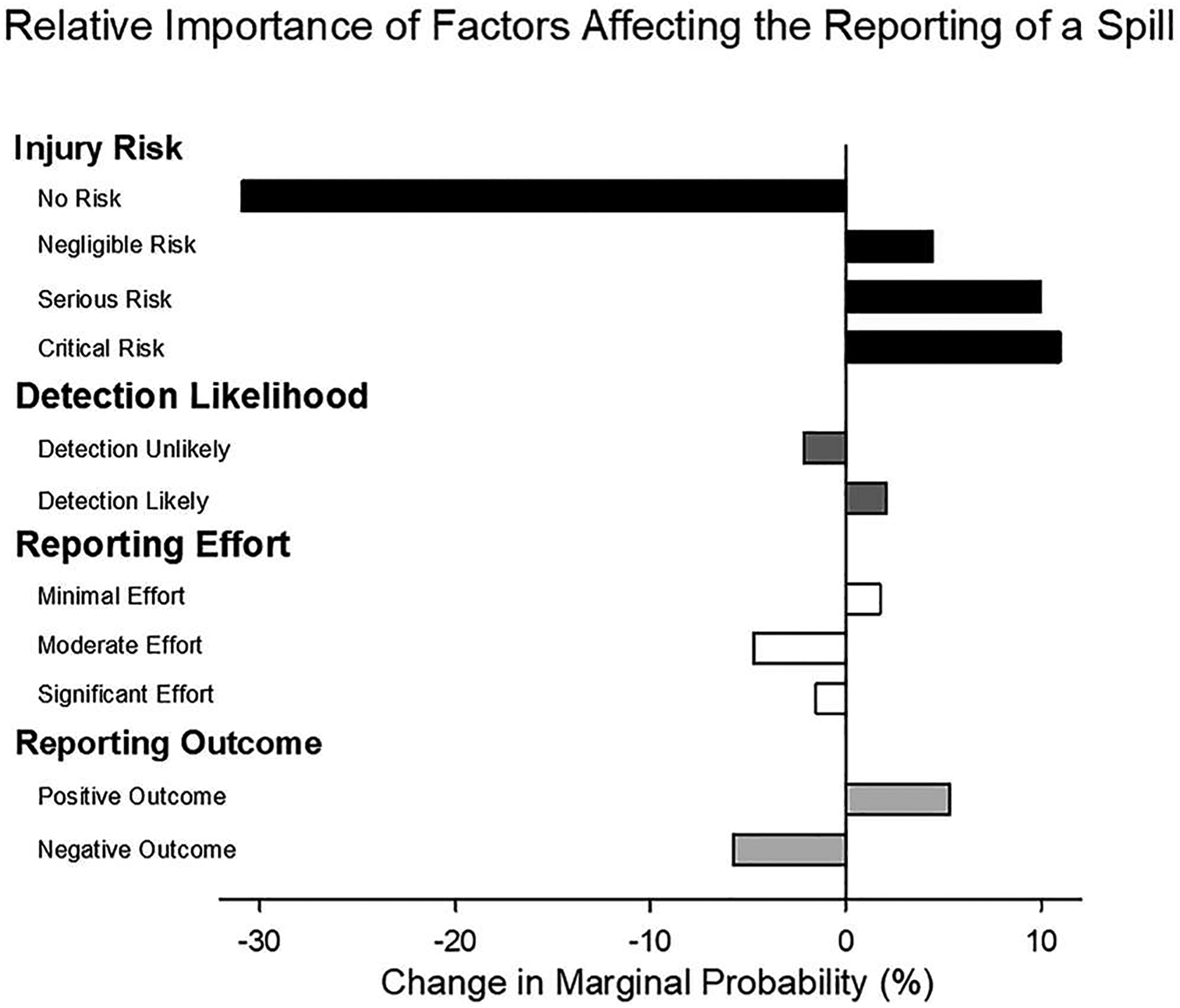
Example DCE marginal probabilities from Wirth et al. (2020). Note: Results of a DCE from Wirth et al. (2020), showing the change in marginal probabilities when choosing an alternative with the specific attribute level relative to the average choice probability on that alternative.

As shown in Fig. 2, this DCE revealed that severity of a potential injury was the most influential factor in safety-related decision making in this sample of laboratory workers. The possibility of critical and serious risk of injury increased the likelihood of reporting an incident. The results also revealed that factors relating to work and social pressures exerted some influence over safety-related decision making in the DCE scenarios. For instance, the likelihood of reporting a safety incident decreased somewhat when there was a potential negative consequence (i.e., a punisher) for reporting the incident or when reporting the incident required some effort. The likelihood of reporting a safety incident in the scenarios was also increased when there was a likelihood of the incident being detected by others.

This example provides a good illustration of the potential relevance and scope of DCEs for behavioral sciences interested in choice and decision-making research. A DCE can be used to extend choice research beyond the traditional analysis of tangible Commodities and goods (and their features or attributes) to the analysis of more nebulous influencing factors such as behavioral, social, or context-related factors and conditions. As shown in the example, the influence of behavioral, social, and organizational pressures can be simulated realistically and simultaneously, making it possible to study the influences of any variety of behavioral and environmental factors derived from behavior analytic theory.

4. Conclusion

The DCE is an economic choice procedure that is fundamentally similar to the methods used to assess choice in psychological research. In both cases, the goal of the procedures is to understand how the features of reinforcers and other behavioral outcomes affect choice. Both economists and psychologists assume that distribution of choice is best quantified by the relative distribution of the outcome value or utility (Eqs. 2 and 10). In both areas of study, respondents are most often asked to report choices they would make in hypothetical scenarios. Although in both fields, choice is studied in experiments in which participants will actually receive the outcomes. There is generally good concordance between hypothetical and “real” behavior in both fields (Madden et al., 2003; Quaife, Terris-Prestholt et al., 2018).

There are several divergences between DCE methods and behavior analytic methods, and they vary in scale. As a relatively minor difference, it may be easier to study the effect of categorical variables (e.g., reinforcer quality, types of potential side effects from a vaccine, or positive or negative outcomes for reporting a spill) on choice with a DCE than with a matching-law-based approach. With a DCE, the categorical variable need only be systematically manipulated across choice profiles and choice sets. In comparison, a discounting based method requires measuring the distribution of choice separately across each categorical variable. For example, to measure how people make choices for alcohol, entertainment, and food, Friedel et al. (2014) separately measured the distribution of choices for each commodity in independent assessments.⁴ A matching law based approach requires at least dozens of trials per subject, whereas a DCE approach relies on the law of large numbers by focusing on the population.

Another important difference between DCE methods and behavior analytic methods, is that DCEs are aimed at understanding choice as it exists within a population, whereas behavior analytic studies of choice are focused on understanding choice in an individual subject. For this reason, a common end goal of DCEs is to predict choice at the population level or to determine what choice alternative will have the greatest utility for the most people given some constraint. For example, DCEs in health economics have been used to identify the most desirable treatment based on efficacy balanced against the cost of that treatment.

Beyond considerations about behavior being a phenomenon of the individual (Sidman, 1960) or choice as a population-level measure (McFadden, 1974), an important question is whether a focus on the individual versus the population would lead to a fundamentally different pattern of results. That is, will predictions at one level be the same at the other level? We feel it is reasonable to assume that a stochastic pattern of choice at the individual level (e.g., McLean et al., 2014) would be mirrored by a stochastic pattern of choice at the population level (e.g., Hensher et al., 2015). Imagine a conventional matching experiment with 1000 subjects in which responding is allocated between two alternatives, A or B. Now imagine that a single response, from each subject, that occurs 15 min into a session quantifies choice. If the rate of reinforcement is 2:1 for responses on A versus B, then subjects will spend twice as much time responding to A than responding to B (Baum and Rachlin, 1969). If we capture the behavior of all the subjects in one instant, we should expect twice as many subjects responding A than to B (all else being equal) simply because each subject typically spends twice as much time responding to A. A DCE captures an instantaneous choice by an individual. It is not required nor assumed that the individual will always make that specific response. However, the instantaneous choice of all the individuals in the sample reflect the relative Utilities associated with those choice outcomes. Thus, matching behavior and DCE choice behavior should be related.

Despite the fundamental difference in scope (e.g., population vs. individual), there are potential benefits of DCEs for behavior analysts. For example, an important practical benefit of DCE focusing on the effects of different factors and levels on choice in the population may be helpful in terms of disseminating results. That is, a consumer of research that expects large sample sizes and is uninformed regarding the utility of single-subject designs will be more likely to readily accept the results of a DCE than the results of a matching study. Additionally, there are often research questions pertaining to phenomena at the level of the population. As mentioned above, in some health economics research, the goal is to understand how a set of services might be utilized by a population of consumers. In some transportation research, the question is similar: how will a set of transportation options be used by the local populace? As an example, one practical outcome of our DCE study outlined in Section 3 (Wirth et al., 2020) was that putative reinforcers (i.e., positive feedback from a Supervisor) were related to an increased likelihood that someone will report a potentially unsafe Situation at work. It should be obvious to a behavioral audience that a reinforcer—by definition—leads to increased behavior. The relations between consequences and behavior may be obvious to a behavior analyst that are novel to an audience that has not historically consumed single-subject experimental research (for example, Daniels and Lattal, 2017 discuss the PIC/NIC analysis for organizations, which focuses on identifying effective feedback to employees by focusing on reinforcers vs. punishers, consequence immediacy, and consequence likelihood). A population-level analysis of choice should not be rejected de novo especially if dissemination of Science is a goal. There are likely some research questions for which DCE may be a more effective strategy (e.g., McFadden, 1974), for example trying to determine the factors that could affect the choice to report a safety incident in situations that have never occurred (e.g., a spilled compound poses a critical risk to health; Wirth et al., 2020). Although there are necessarily differences in a utility-based a reinforcer-value based interpretations of choice, there should be a concordance between reinforcer value and systematic utility. We are not intending to suggest that behavior analysts abandon single-subject experimental designs and only use a technique that is specifically designed to understand choice at a population level. We hoped to highlight a research tool that we have found useful and that has been growing in popularity in a variety of fields interested in choice.

It is not possible to cover all aspects of conducting DCEs in a single paper. For example, the International Society for Pharmacoeconomics and Outcomes Research has published three papers providing instructions and best practices for conducting a DCE (Bridges et al., 2011; Hauber et al., 2016; Johnson et al., 2013). Two widely referenced texts on DCEs, Hensher et al. (2015) and Louviere, Hensher et al. (2010), are a combined 1565 page and the SAS documentation related only to DCE is 187 pages (Kuhfeld, 2010). Instead of covering every facet of DCE methodology, we have provided enough details and context for a behavioral and psychological audience. We hope that such readers will be able to appreciate the similarities and differences between traditional matching-law-based approaches to studying choice and DCEs. We also hope that this paper will serve as a primer for readers interested in conducting DCEs.

References

- Ayer AJ, 1954. Philosophical Essays. St. Martin’s Press. [Google Scholar]
- Baum WM, 1974. On two types of deviation from the matching law: bias and undermatching. J. Exp. Anal. Behav 22 (1), 231–242. 10.1901/jeab.1974.22-231. [DOI] [PMC free article] [PubMed] [Google Scholar]
- Baum WM, Rachlin HC, 1969. Choice as time allocation. J. Exp. Anal. Behav 12 (6), 861–874. 10.1901/jeab.1969.12-861. [DOI] [PMC free article] [PubMed] [Google Scholar]
- Beulen L, Grutters JP, Faas BH, Feenstra I, Groenewoud H, van Vugt JM, Bekker MN, 2015. Women’s and healthcare Professionals’ preferences for prenatal testing: a discrete choice experiment. Prenat. Diagn 35 (6), 549–557. 10.1002/pd.4571. [DOI] [PubMed] [Google Scholar]
- Bridges JF, Hauber AB, Marshall D, Lloyd A, Prosser LA, Regier DA, Johnson FR, Mauskopf J, 2011. Conjoint analysis applications in health-a checklist: a report of the ISPOR Good Research Practices for Conjoint Analysis Task Force. Value Health 14 (4), 403–413. 10.1016/j.jval.2010.11.013. [DOI] [PubMed] [Google Scholar]
- Catania AC, 2007. Learning, Fourth Interim ed. Sloan. [Google Scholar]
- Centers for Disease Control and Prevention, 1997. Evaluation of safety devices for preventing percutaneous injuries among health-care workers during phlebotomy procedures-Minneapolis-St. Paul, New York City, and San Francisco, 1993–1995. MMWR: Morb. Mortal. Wkly. Rep 46 (2), 21–25. [PubMed] [Google Scholar]
- Cohen H, Cohen P, West SG, Aiken LS, 2003. Applied Multiple Regression/Correlation Analysis for the Behavioral Sciences, 3 ed. Routledge. [Google Scholar]
- Crouch GI, Louviere JJ (2001). A review of Choice Modelling research in tourism, hospitality and leisure. 67–86. ( 10.1079/9780851995359.0067). [DOI] [Google Scholar]
- Cunningham CE, Bruce BS, Snowdon AW, Chen Y, Kolga C, Piotrowski C, Warda L, Correale H, Clark E, Barwick M, 2011. Modeling improvements in booster seat use: a discrete choice conjoint experiment. Accid. Anal. Prev 43 (6), 1999–2009. 10.1016/j.aap.2011.05.018. [DOI] [PubMed] [Google Scholar]
- Daniels AC, Lattal AD, 2017. Life is a PIC/NIC:.When You Understand Behaviour. Sloan. [Google Scholar]
- Dasaolu BO, Obasola KE, 2019. A religio-philosophical analysis of freewill and determinism in relation to the Yoruba perception of Ori. Oguaa J. Relig. Hum. Values 5 (2), 5975. [Google Scholar]
- Davies B, 2014. Thomas Aquinas’s Summa Theologiae: A Guide and Commentary. Oxford University Press, New York: (Incorporated). [Google Scholar]
- DeHart WB, Friedel JE, Berry M, Frye CCJ, Galizio A, Odum AL, 2020. Comparison of delay discounting of different outcomes in cigarette smokers, smokeless tobacco users, e-cigarette users, and non-tobacco users. J. Exp. Anal. Behav 114 (2), 203–215. 10.1002/jeab.623. [DOI] [PMC free article] [PubMed] [Google Scholar]
- Dong D, Xu RH, Wong EL, Hung CT, Feng D, Feng Z, Yeoh EK, Wong SY, 2020. Public preference for COVID-19 vaccines in China: a discrete choice experiment. Health Expect. 23 (6), 1543–1578. 10.1111/hex.13140. [DOI] [PMC free article] [PubMed] [Google Scholar]
- Ferster C, Skinner B, 1957. Schedules of Reinforcement. Appleton-Century-Crofts. [Google Scholar]
- Foreman AM, Friedel JE, Hayashi Y, Wirth O, 2021. Texting while driving: a discrete choice experiment. Accid. ; Anal. Prev 149, 105823 10.1016/j.aap.2020.105823. [DOI] [PMC free article] [PubMed] [Google Scholar]
- Friedel JE, DeHart WB, Madden GJ, Odum AL, 2014. Impulsivity and cigarette smoking: discounting of monetary and consumable outcomes in current and non-smokers. Psychopharmacology 231 (23), 4517–4526. 10.1007/s00213-014-3597-z. [DOI] [PMC free article] [PubMed] [Google Scholar]
- Glenngard AH, Hjelmgren J, Thomsen PH, Tvedten T, 2013. Patient preferences and willingness-to-pay for ADHD treatment with stimulants using discrete choice experiment (DCE) in Sweden, Denmark and Norway. Nord J. Psychiatry 67 (5), 351–359. 10.3109/08039488.2012.748825. [DOI] [PubMed] [Google Scholar]
- Hanmer MJ, Kalkan KO, 2013. Behind the curve: clarifying the best approach to calculating predicted probabilities and marginal effects from limited dependent variable models. Am. J. Political Sci 57 (1), 263–277. 10.1111/j.1540-5907.2012.00602.x. [DOI] [Google Scholar]
- Hauber AB, Gonzalez JM, Groothuis-Oudshoom CG, Prior T, Marshall DA, Cunningham C, MJ IJ, Bridges JF, 2016. Statistical methods for the analysis of discrete choice experiments: a report of the ISPOR conjoint analysis good research practices task force. Value Health 19 (4), 300–315. 10.1016/j.jval.2016.04.004. [DOI] [PubMed] [Google Scholar]
- Hensher DA, Greene WH, 2003. The mixed logit model: the state of practice. Transportation 30 (2), 133–176. 10.1023/a:1022558715350. [DOI] [Google Scholar]
- Hensher DA, Rose JM, Greene WH, 2015. Applied Choice Analysis: A Primer. Cambridge University Press. [Google Scholar]
- Herrnstein RJ, 1961. Relative and absolute strength of response as a function of frequency of reinforcement. J. Exp. Anal. Behav 4, 267–272. 10.1901/jeab.l961.4-267. [DOI] [PMC free article] [PubMed] [Google Scholar]
- Herrnstein RJ, 1970. On the law of effect. J. Exp. Anal. Behav 13 (2), 243–266. 10.1901/jeab.1970.13-243. [DOI] [PMC free article] [PubMed] [Google Scholar]
- Hollard V, Davison MC, 1971. Preference for qualitatively different reinforcers. J. Exp. Anal. Behav 16 (3), 375–380 https://doi.org/jeab.1971.16-375. [DOI] [PMC free article] [PubMed] [Google Scholar]
- Johnson FR, Lancsar E, Marshall D, Kilambi V, Muhlbacher A, Regier DA, Bresnahan BW, Kanninen B, Bridges JF, 2013. Constructing experimental designs for discrete-choice experiments: report of the ISPOR Conjoint Analysis Experimental Design Good Research Practices Task Force. Value Health 16 (1), 3–13. 10.1016/j.jval.2012.08.2223. [DOI] [PubMed] [Google Scholar]
- Kuhfeld WF, 2010. Experimental design: efficiency, coding, and choice designs. Marketing Research Methods in SAS: Experimental Design, Choice, Conjoint, and Graphical Techniques. SAS, pp. 53–240. (http://supportsas.com/techsup/technote/mr2010.pdf). [Google Scholar]
- Lancsar E, Louviere J, Flynn T, 2007. Several methods to investigate relative attribute impact in stated preference experiments. Soc. Sci. Med 64 (8), 1738–1753. 10.1016/j.socscimed.2006.12.007. [DOI] [PubMed] [Google Scholar]
- Lin A, 2013. Classroom code-switching: three decades of research. Appl. Linguist. Rev 4 (1), 195–218. 10.1515/applirev-2013-0009. [DOI] [Google Scholar]
- Lipscomb HJ, Nolan J, Patterson D, Sticca V, Myers DJ, 2013. Safety, incentives, and the reporting of work-related injuries among union carpenters: “you’re pretty much screwed if you get hurt at work”. Am. J. Ind. Med 56 (4), 389–399. 10.1002/ajim.22128. [DOI] [PubMed] [Google Scholar]
- Louviere JJ, Hensher DA, Swait JD, 2010. Stated Choice Methods. Cambridge University Press, 10.1017/cbo9780511753831. [DOI] [Google Scholar]
- Louviere JJ, Flynn TN, Carson RT, 2010. Discrete choice experiments are not conjoint analysis. J. Choice Model 3 (3), 57–72. 10.1016/s1755-5345(13)70014-9. [DOI] [Google Scholar]
- Luce RD, Tukey JW, 1964. Simultaneous conjoint measurement: a new type of fundamental measurement. J. Math. Psychol 1 (1), 1–27. 10.1016/0022-2496(64)90015-x. [DOI] [Google Scholar]
- Madden GJ, Begotka AM, Raiff BR, Kastern LL, 2003. Delay discounting of real and hypothetical rewards. Exp. Clin. Psychopharmacol 11 (2), 139–145. 10.1037/1064-1297.11.2.139. [DOI] [PubMed] [Google Scholar]
- Mazur JE, 1987. An adjusting procedure for studying delayed reinforcement. In: Commons ML, Mazur JE, Nevin JA, Rachlin H (Eds.), Quantitative analysis of behavior: Vol. 5. The effect of delay and intervening events on reinforcement value. Earlbaum, pp. 55–73. [Google Scholar]
- McDowell JJ, 2005. On the classic and modern theories of matching. J. Exp. Anal. Behv 84 (1), 111–127. 10.1901/jeab.2005.59-04. [DOI] [PMC free article] [PubMed] [Google Scholar]
- McFadden D, 1974. Conditional logit analysis of qualitative choice behavior. In: Zarembka P (Ed.), Frontiers in econometrics. Academic Press. [Google Scholar]
- McLean AP, Grace RC, Pitts RC, Hughes CE, 2014. Preference pulses without reinforcers. J. Exp. Anal. Behav 101 (3), 317–336. 10.1002/jeab.84. [DOI] [PubMed] [Google Scholar]
- Miller HL, 1976. Matching-based hedonic scaling in the pigeon. J. Exp. Anal. Behav 26 (3), 335–347. 10.1901/jeab.1976.26-335. [DOI] [PMC free article] [PubMed] [Google Scholar]
- Neef NA, Mace FC, Shea MC, Shade D, 1992. Effects of reinforcer rate and reinforcer quality on time allocation: extensions of matching theory to educational settings. J. Appl. Behav. Anal 25 (3), 691–699. 10.1901/jaba.1992.25-691. [DOI] [PMC free article] [PubMed] [Google Scholar]
- Norton EC, Dowd BE, Maciejewski ML, 2019. Marginal effects-quantifying the effect of changes in risk factors in logistic regression models. JAMA 321 (13), 1304–1305. 10.1001/jama.2019.1954. [DOI] [PubMed] [Google Scholar]
- Plato. (1993). The Republic (Jowett B, Trans.). Auckland: Floating Press, The. [Google Scholar]
- Pransky G, Snyder T, Dembe A, Himmelstein J, 1999. Under-reporting of work-related disorders in the workplace: a case study and review of the literature. Ergonomics 42 (1), 171–182. 10.1080/001401399185874. [DOI] [PubMed] [Google Scholar]
- Quaife M, Terris-Prestholt F, Di Tanna GL, Vickerman P, 2018. How well do discrete choice experiments predict health choices? A systematic review and meta-analysis of external validity. Eur. J. Health Econ 19 (8), 1053–1066. 10.1007/s10198-018-0954-6. [DOI] [PubMed] [Google Scholar]
- Quaife M, Eakle R, Cabrera Escobar MA, Vickerman P, Kilbourne-Brook M, Mvundura M, Delany-Moretlwe S, Terris-Prestholt F, 2018. Divergent preferences for HIV prevention: a discrete choice experiment for multipurpose HIV prevention products in south Africa. Med. Decis. Mak 38 (1), 120–133. 10.1177/0272989X17729376. [DOI] [PubMed] [Google Scholar]
- Rachlin H, 1971. On the tautology of the matching law. J. Exp. Anal. Behav 15 (2), 249–251. 10.1901/jeab.1971.15-249. [DOI] [PMC free article] [PubMed] [Google Scholar]
- Rachlin H, Raineri A, Cross D, 1991. Subjective probability and delay. J. Exp. Anal. Behav 55 (2), 233–244. 10.1901/jeab.1991.55-233. [DOI] [PMC free article] [PubMed] [Google Scholar]
- Ryan M, Yi D, Avenell A, Douglas F, Aucott L, van Teijlingen E, Vale L, 2015. Gaining pounds by losing pounds: preferences for lifestyle interventions to reduce obesity. Health Econ. Policy Law 10 (2), 161–182. 10.1017/S1744133114000413. [DOI] [PubMed] [Google Scholar]
- Samuelson PA, 1937. A note on measurement of utility. Rev. Econ. Stud 4 (2), 155–161. 10.2307/2967612. [DOI] [Google Scholar]
- Sidman M, 1960. Tactics of scientific research. Authors Cooperative, Inc. [Google Scholar]
- Thurstone LL, 1927. A law of comparative judgment. Psychol. Rev 34 (4), 273–286. 10.1037/h0070288. [DOI] [Google Scholar]
- Truong TP, Hensher DA, 1985. Measurement of travel time values and opportunity cost from a discrete-choice model. Econ. J 95 (378), 438. 10.2307/2233219. [DOI] [Google Scholar]
- Voide C, Darling KE, Kenfak-Foguena A, Erard V, Cavassini M, Lazor-Blanchet C, 2012. Underreporting of needlestick and sharps injuries among healtheare workers in a Swiss University Hospital. Swiss Med. Wkly 142, 13523. 10.4414/smw.2012.13523. [DOI] [PubMed] [Google Scholar]
- Vollmer TR, Bourret J, 2000. An application of the matching law to evaluate the allocation of two- and three-point shots by College basketball players. J. Appl. Behav. Anal 33 (2), 137–150. 10.1901/jaba.2000.33-137. [DOI] [PMC free article] [PubMed] [Google Scholar]
- Wenzel C, Marchal K, 2017. Chinese perspectives on free will. In: Timpe K, Griffith M, Levy N (Eds.), The Routledge Companion to Free Will. Routledge, pp. 374–388. 10.4324/9781315758206.ch34. [DOI] [Google Scholar]
- Windsor J, Piché LM, Locke PA, 1994. Preference testing: a comparison of two presentation methods. Res. Dev. Disabil 15 (6), 439–455. 10.1016/0891-4222(94)90028-0. [DOI] [PubMed] [Google Scholar]
- Wirth O, Foreman AM, Friedel JE, Andrew ME, 2020. Two discrete choice experiments on laboratory safety decisions and practices. J. Saf. Res 75, 99–110. 10.1016/j.jsr.2020.08.005. [DOI] [PMC free article] [PubMed] [Google Scholar]