

Abstract
The analysis of the relationship between time and cost is a crucial aspect of construction project management. Various optimization techniques have been developed to solve time–cost trade-off problems. A hybrid multi-verse optimizer model (hDMVO) is introduced in this study, which combines the multi-verse optimizer (MVO) and the sine cosine algorithm (SCA) to address the discrete time–cost trade-off problem (DTCTP). The algorithm's optimality is evaluated by using 23 well-known benchmark test functions. The results demonstrate that hDMVO is competitive with MVO, SCA, the dragonfly algorithm and ant lion optimization. The performance of hDMVO is evaluated using four benchmark test problems of DTCTP, including two medium-scale instances (63 activities) and two large-scale instances (630 activities). The results indicate that hDMVO can provide superior solutions in the time–cost optimization of large-scale and complex projects compared to previous algorithms.
Subject terms: Civil engineering, Computational science
Introduction
In project management, optimization is a highly useful tool to satisfy desired objectives under specific constraints. The productivity of different components of a project can be increased by optimization. The importance of optimization in a construction project has been emphasized for decades as it is used to find the ideal plan and schedule for completing a project. Cost optimization, time optimization, and Pareto front are three common forms of time–cost trade-off problems. The objective of the cost optimization problem is to minimize the total cost under specific conditions, including project implementation time and penalty costs for delays. Meanwhile, the time optimization problem is aimed at choosing alternative solutions to shorten the project implementation time while ensuring that the project cost does not exceed the revenue on the early operation of the project. The Pareto front is a multi-objective optimization problem to simultaneously optimize both project cost and time1.
Mirjalili, Mirjalili2 proposed a multi-verse optimizer (MVO) algorithm inspired by the Big Bang theory to satisfy the need for solving single-and multi-objective optimization problems. For result assessment, MVO is compared with other metaheuristic algorithms, such as particle swarm optimization (PSO), Genetic Algorithm (GA), Ant colony optimization (ACO), etc. The results show that the MVO algorithm can provide competitive, even superior results than those of other algorithms in most tested optimization problems. However, MVO has issues in balancing the exploration and exploitation mechanism of the search area and limitations in the search area exploitation during fast convergence, thus resulting in local optimization3.
The Sine Cosine Algorithm (SCA)4 was developed for focusing on the exploration and exploitation of the search space during optimization. The results of the test problems show that SCA can explore different regions of the search space, avoid local optimization, converge towards global optimization, and effectively exploit the promising region of the search space during optimization. In addition, the study shows that SCA converges significantly faster than PSO, GA, ACO, etc. SCA has been utilized to address optimization challenges in diverse domains since 20165. Like MVO, SCA has limitations. Specifically, its search area exploitation mechanism is not clearly expressed; therefore, it easily encounters fast convergence6, which results in local optimization.
Two algorithms with opposite advantages and disadvantages motivated us to develop a hybrid algorithm between MVO and SCA for optimal exploration and exploitation of the search area based on the strengths of each algorithm to achieve a balance between the two mechanisms. The hDMVO algorithm was developed by preserving MVO's mechanisms of white and black holes to ensure good exploration of the search area by MVO. Concurrently, good search area exploitation by the algorithm is guaranteed by SCA through the fact that the value closest to the global optimum is stored in a variable as the target and is never lost during the optimization. Therefore, hDMVO will achieve a reasonable balance between the exploration and the exploitation phases, which ensures that the algorithm can achieve global optimization and become an appropriate metaheuristic method for solving the DTCTP.
The resolution of large-scale DTCTPs is a crucial aspect in the management of any construction project. Despite the availability of several existing methods, they are not fully equipped to solve large-scale DTCTPs. Therefore, a hybrid multi-verse optimizer model (hDMVO) was developed by combining the MVO and the SCA to provide efficient solutions for medium- and large-scale DTCTPs and other optimization problems that can be applied in actual construction projects. This model also significantly enhances the decision-making ability of decision-makers.
The rest of this paper is organized as follows. Section "Literature review" summarizes the literature on the time–cost trade-off problems. Section "Model development" outlines the development of our hybrid multi-verse optimizer model. Section "Computational experiments" presents the results from the validation and application of our model. Finally, Sections "Conclusion" and "Recommendations for future work" conclude the study and outline future research directions.
Literature review
The stochastic optimization method is widely used in many fields of study7,8, which develops meta-heuristic techniques. Some popular meta-heuristic methods are inspired by animals in nature. For example, ant lion optimization (ALO) algorithm is modeled after the hunting behavior of antlions in nature. The Dragonfly algorithm (DA) is based on the static and dynamic swarming behaviors observed in dragonflies9. Africa Wild Dog Optimization Algorithm (AWDO) originates from the hunting mechanism of Africa wild dogs in nature10. Meanwhile, Genetic Algorithm (GA) is inspired by evolutionary principles, such as heredity, mutation, natural selection, and crossover11.
The development of new algorithms or improvement of current algorithms has recently attracted immense interest from researchers, which is related to the No Free Lunch (NFL) theorem12. Evidently, the NFL has enabled researchers to improve and adapt current algorithms for solving different problems or propose new algorithms to provide competitive results against current algorithms. There are a significant number of developed hybrid metaheuristic algorithms, including the ant colony system-based decision support system (ACS-SGPU)13, dragonfly algorithm–particle swarm optimization model14, quantum-based sine cosine algorithm15, the improved sine–cosine algorithm based on orthogonal parallel information16, the hybrid sine cosine algorithm with multi-orthogonal search strategy17.
The time–cost trade-off is extended to the discrete version, including various realistic assumptions and solved by the exact, heuristic, and metaheuristic methods. PSO and GA are metaheuristic methods commonly used in the DTCTP. Bettemir18 found that among eight metaheuristic methods, including a sole genetic algorithm, four hybrid genetic algorithms, PSO, ant colony optimization, and electromagnetic scatter search, PSO was one of the leading algorithms together with the hybrid genetic algorithm with quantum annealing for the large-scale cost optimization. Zhang and Xing19 proposed an algorithm combining PSO and fuzzy sets theory to solve the fuzzy time–cost–quality trade-off problem. Aminbakhsh and Sonmez20 developed the discrete particle swarm optimization method to solve the large-size time–cost trade-off problem. Aminbakhsh and Sonmez21 used Pareto front particle swarm optimizer (PFPSO) to simultaneously optimize the time and cost of large-scale projects. Sonmez and Bettemir22 presented a hybrid strategy based on GAs, simulated annealing, and quantum simulated annealing techniques for the cost optimization problem. Zhang et al.23 proposed a GA for the DTCTP in repetitive projects. Naseri and Ghasbeh24 used GA for the time–cost trade off analysis to compensate for project delays. Network analysis algorithm is also metaheuristic techniques used to solve the DTCTP25. Son and Khoi26 presented a slime mold algorithm model to solving time–cost–quality trade-off problem.
Despite their wide applications in solving the DTCTP, the metaheuristic techniques have several limitations. Therefore, hybrid metaheuristic methods are being developed and widely used in the DTCTP. An adaptive-hybrid genetic algorithm was proposed by Zheng27 for time–cost–quality trade-off problems. Said and Haouari28 developed a model wherein the simulation–optimization strategy and the mixed-integer programming formulation were used to solve the DTCTP. Tran, Luong-Duc29 presented an opposition multiple objective symbiotic organisms search (OMOSOS) model for time, cost, quality, and work continuity trade-off in repetitive projects. Eirgash et al.30 proposed a multi-objective teaching–learning-based optimization algorithm integrated with a nondominated sorting concept (NDS–TLBO), which is successfully applied to optimize the medium- to large-scale projects. A hybrid GALP algorithm combined with GA and linear programming (LP) was proposed by Alavipour and Arditi31 for time–cost tradeoff analysis. Albayrak32 developed an algorithm combining PSO and GA to solve the time–cost trade-off problem for resource-constrained construction projects. A population-based metaheuristics approach, nondominated sorting genetic algorithm III (NSGA III) was developed by Sharma and Trivedi33 to ensure the quality and safety in time–cost trade-off optimization. Li et al.34 presented an epsilon-constraint method-based genetic algorithm for uncertainty multimode time–cost–robustness trade-off problem.
This paper presents a hybrid multi-verse optimizer (hDMVO) model based on MVO and SCA, which can provide high-quality solutions for large-scale discrete time–cost trade-off optimization problems.
Model development
Discrete time–cost trade-off problem
The common objective of discrete time–cost tradeoff problem (DTCTP) is to minimize the total direct and indirect costs and such costs can be formulated as follows35:
| 1 |
subject to:
| 2 |
| 3 |
| 4 |
where C is the project cost; dcjk is the direct cost of mode k for activity j; xjk is a 0–1 variable which is 1 if mode k is selected for executing activity j, and 0 otherwise; ic is the daily indirect cost; D is the project duration; djk is the duration of mode k for activity j; Stj is the start time for activity j; and Scj is the set of immediate successors for j.
Hybrid multi-verse optimizer model for DTCTP
Multi-verse optimizer—MVO
The MVO algorithm is inspired by concepts which theoretically exist in astronomy, including white holes, black holes, and worm holes. White holes are the elements which form the universes and have been unobservable until now. Meanwhile, black holes are observable and characterized by a giant gravitational force which attracts all surrounding objects. The last element can exchange objects between different universes or different parts of a universe. In the MVO, the above three elements are mathematically modeled to develop an optimal method, simulate the teleportation and exchange of objects between universes through white/black and worm hole tunnels. In addition, the idea of the inflation of the universe is also applied to the MVO based on the inflation rate.
The model of the MVO algorithm is shown in Fig. 1. In this figure, the universe with a higher inflation rate will have a white hole, while a universe with a lower inflation rate will have a black hole. The objects will then be transferred from the white holes of the source universe to the black holes of the target universe. In order to improve the overall inflation rate of single universes, an assumption was made that the universes with high inflation rate would be more likely to have white holes. In contrast, the universes with low inflation rate are more likely to have black holes. In Fig. 1, the white points represent celestial bodies travelling through the worm holes. It can be observed that worm holes stochastically change celestial bodies regardless of their inflation rates.
Figure 1.

Conceptual model of the proposed MVO algorithm.
The roulette wheel mechanism will be used. (Eq. 6) to mathematically model white or black hole tunnels and exchange celestial objects between universes. When optimization problems are solved with the maximized objective function, –NI will be changed into NI. In each iteration, universes will be rearranged based on their inflation rate (fitness value), and by the roulette wheel mechanism, one universe will be selected in the occurrence of white hole, assume that:
| 5 |
where d is the number of parameters (variables) and n is the number of universes (candidate solutions):
| 6 |
where indicates the jth parameter of ith universe, Ui shows the ith universe, NI(Ui) is normalized inflation rate of the ith universe, r1 is a random number in [0, 1], and indicates the jth parameter of kth universe selected by a roulette wheel selection mechanism.
With the above-mentioned mechanism, universes keep the objects exchanged without interference. For accurate determination of the diversity of universes and exploitation, each universe has a wormhole to stochastically transport its objects through space. In order to provide local changes for each universe and improve inflation rate by using wormholes, worm hole tunes are assumed to always be established between a universe and a best universe formed so far. This mechanism is presented as follows:
| 7 |
where Xj indicates the jth parameter of best universe formed so far, TDR is a coefficient, WEP is another coefficient, lbj shows the lower bound of jth variable, ubj is the upper bound of jth variable, indicates the jth parameter of ith universe, and r2, r3, r4 are random numbers in [0, 1].
Two main coefficients, namely the wormhole existence probability (WEP) and travelling distance rate (TDR) can be seen in Eq. (7). The coefficient WEP was used to determine the wormhole existence probability in the universe. Such coefficient will linearly increase over the iterations (Eq. 8).
| 8 |
where the min variable is the minimum value, the max variable is the maximum value, l presents the number of the current iteration, and L presents the termination criteria (the maximum number of iterations).
TDR is a factor to determine the distance rate (variation) by which an object can be displaced by a wormhole around the best universe formed so far. (Eq. 9). In contrast to WEP, TDR decreases over iterations for more precise exploitation or local search around the best universe formed so far (Fig. 2).
| 9 |
where p presents the exploitation rate through the iterations. The larger p, the earlier and more precise exploitation/local search.
Figure 2.
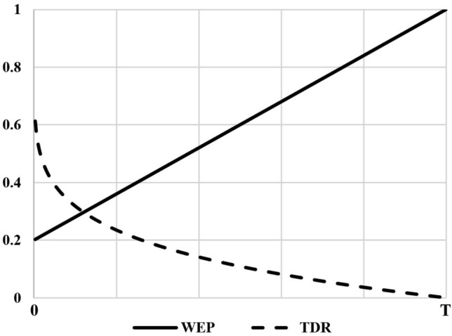
Wormhole existence probability (WEP) versus travelling distance rate (TDR).
In the MVO algorithm, the optimization process starts with generating a set of random universes. At each iteration, objects in universes with higher inflation rates tend to travel to universes with lower inflation rates through white or black holes. Meanwhile, every universe has to face random processes of celestial bodies through wormholes to reach the best universe. This process is repeated until the termination criteria are satisfied (such as a predetermined maximum number of iterations).
Sine cosine algorithm-SCA
Stochastic population-based techniques have in common is to divide the optimization process into two phases: exploration and exploitation36. In the exploration phase, the optimization algorithm will abruptly combine solutions with a high random rate to find the promising region of the search space. However, in the exploitation phase, there will be gradual changes in the stochastic solutions, and the stochastic variations will be significantly less than those in the exploration phase.
In SCA, the mathematical equations for updating positions are given for both phases, see Eqs. (10) and (11):
| 10 |
| 11 |
where is the position of the current solution in ith dimension at tth iteration, α1, α2 and α3 are random numbers, is position of the destination point in ith dimension, and || indicates the absolute value.
The above two formulas are combined into a general formula as follows:
| 12 |
where α4 is a random number in [0,1].
In Eq. (12), it can be seen that SCA has 4 main parameters: α1, α2, α3, and α4. α1 defines the movement direction, α2 determines how far the movement should be towards or outwards the destination, α3 denotes random weights for destination. Finally, the parameter α4 switches between the sine and cosine components in Eq. (12).
A general model in Fig. 3 shows the effectiveness of the sine and cosine functions in the range [− 2, 2]. This figure shows how the range of sine and cosine changes in order to update the location of a response. Randomness is also achieved by determining a random number for α2 in [0, 2π] (Eq. (12)). Therefore, this mechanism ensures the exploration of the search space.
Figure 3.

Sine and cosine with the range in [− 2, 2] allow a solution to go around (inside the space between them) or beyond (outside the space between them) the destination.
In each iteration, the range of Sine and Cosine functions in Eqs. (10)–(12) will be changed to balance the exploitation and exploration phases in order to find the promising regions of the search space and finally achieve the global optimization by Eq. (13):
| 13 |
where v is a constant, t is the current iteration and T is the maximum number of iterations. Figure 4 shows the reduction in the range of the sine and cosine functions over the course of iterations.
Figure 4.

Decreasing pattern for range of sine and cosine.
Hybrid multi-verse optimizer model for DTCTP
By taking advantage of SCA and MVO, the hDMVO is built to change the MVO's exploitation mechanism by the SCA's exploitation mechanism while preserving the MVO’s mechanisms of roulette wheel selection Eq. (14), thereby improving the hDMVO's search area exploration and exploitation.
| 14 |
where indicates the jth parameter of ith universe, Ui shows the ith universe, NI(Ui) is normalized inflation rate of the ith universe, δ1 is a random number in [0, 1], and indicates the jth parameter of kth universe selected by a roulette wheel selection mechanism.
A new formula which combines two algorithms MVO and SCA will be developed from Eq. (9) and Eq. (12) as follows:
| 15 |
where Xj indicates the jth parameter of best universe formed so far. TDR is wormhole existence probability was calculated by Eq. (8) with min = 0.2 and max = 3. WEP is travelling distance rate was calculated by Eq. (9) with p = 10. lbj shows the lower bound of jth variable, ubj is the upper bound of jth variable, indicates the jth parameter of ith universe, and δ2, δ3, δ4 are random numbers in [0, 1]. δ5 are also random numbers in [0, 2π]. The parameter δ5 defines how far the movement should be towards or outwards the destination. The pseudo-code and flowchart of our hDMVO method is given in Figs. 5 and 6. The set of parameters that are summarized in Table 1 provided an adequate combination for the hDMVO, MVO and SCA.
Figure 5.

Pseudo-code of the proposed hDMVO algorithm.
Figure 6.
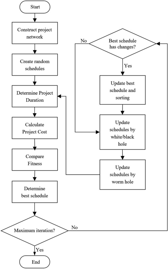
Flowchart of the proposed hDMVO algorithm.
Table 1.
Parameter settings of the hDMVO, SCA and MVO.
| Algorithm | Parameter | Description | Value |
|---|---|---|---|
| hDMVO | N | Number of iterations | 250 |
| i | Number of solutions | 200 | |
| min | Minimum value | 0.2 | |
| max | Maximum value | 3 | |
| p | Exploitation rate | 10 | |
| δ1 | Random number | [0, 1] | |
| δ2 | Random number | [0, 1] | |
| δ3 | Random number | [0, 1] | |
| δ4 | Random number | [0, 1] | |
| δ5 | Random number | [0, 2π] | |
| SCA | N | Number of iterations | 250 |
| i | Number of solutions | 200 | |
| v | Constant value | 3 | |
| α2 | Random number | [0, 2π] | |
| α3 | Random number | [0, 2] | |
| α4 | Random number | [0, 1] | |
| MVO | N | Number of iterations | 250 |
| i | Number of solutions | 200 | |
| min | Minimum value | 0.2 | |
| max | Maximum value | 3 | |
| p | Exploitation rate | 10 | |
| r1 | Random number | [0, 1] | |
| r2 | Random number | [0, 1] | |
| r3 | Random number | [0, 1] | |
| r4 | Random number | [0, 1] |
The complexity of the hDMVO algorithm is influenced by various factors such as the number of activities, schedules, iterations, roulette wheel selection mechanism, and sorting mechanism. The roulette wheel selection method, which is applied for every activity in each solution over the course of iterations, has a complexity of O(log N). The sorting of solutions is carried out at each iteration by utilizing the Quicksort algorithm, which has a complexity of O(N^2) in the worst-case scenario. As a result, the overall computational complexity is:
| 16 |
| 17 |
where n is the number of activities, N is the number of schedules, and T is the maximum iterations.
In the optimization process, the solution a is evaluated to be better than solution b if:
| 18 |
In case the project cost is equal (Ca = Cb), The option with the shortest completion time is considered the best one:
| 19 |
In case both options a and b have the same project cost and project duration, the optimal solution will be stochastically selected.
The exploration and exploitation of the search space will be significantly improved thanks to the hDMVO algorithm. Such hybrid algorithm not only searches for the optimal solution from the sets of solutions stochastically generated at the initial phase, but can also exploit the space between solutions through each iteration to find new promising regions of the search space.
Computational experiments
Convergence behaviours
To assess the optimization capabilities of hDMVO, a comprehensive analysis was conducted using twenty-three well-known benchmark test functions. Comparisons were made to the results obtained from four other optimization algorithms, including MVO, SCA, DA, and ALO. These benchmark functions are grouped into three categories: unimodal, multimodal, and fixed-dimension multi-modal functions, as detailed in Tables 2, 3 and 4.
Table 2.
Uni-modal test functions.
| Funtion | Dim | Range | fmin |
|---|---|---|---|
| 10 | [− 100, 100] | 0 | |
| 10 | [− 10, 10] | 0 | |
| 10 | [− 100, 100] | 0 | |
| 10 | [− 100, 100] | 0 | |
| 10 | [− 30, 30] | 0 | |
| 10 | [− 100, 100] | 0 | |
| 10 | [− 1.28, 1.28] | 0 |
Table 3.
Multi-modal test functions.
| Funtion | Dim | Range | fmin |
|---|---|---|---|
| 10 | [− 500, 500] | –2820.8 | |
| 10 | [− 5.12, 5.12] | 0 | |
| 10 | [− 32, 32] | 0 | |
| 10 | [− 600, 600] | 0 | |
| 10 | [− 50, 50] | 0 | |
| 10 | [− 50, 50] | 0 |
Table 4.
Fixed-dimension multi-modal test functions.
| Funtion | Dim | Range | fmin |
|---|---|---|---|
| 2 | [− 65, 65] | 1 | |
| 4 | [− 5, 5] | 0.0003 | |
| 2 | [− 5, 5] | –1.0316 | |
| 2 | [− 5, 5] | 0.398 | |
| 2 | [− 2, 2] | 3 | |
| 3 | [0, 1] | –3.86 | |
| 6 | [0, 1] | –3.32 | |
| 4 | [0, 10] | –10.1532 | |
| 4 | [0, 10] | –10.4028 | |
| 4 | [0, 10] | –10.5363 |
In order to ensure a fair comparison, all of the algorithms were executed 30 times for each benchmark function. Statistical results, including the mean value (ave) and standard deviation (std), were collected from 30 runs of the algorithm. It is important to note that 30 search agents and a maximum of 500 iterations were utilized in the analysis. The statistical results of the hDMVO algorithm, as well as those of other comparative algorithms (DA, ALO, SCA, and MVO), can be found in Tables 5, 6 and 7.
Table 5.
Results of unimodal benchmark functions.
| F | hDMVO | MVO | SCA | DA | ALO | |||||
|---|---|---|---|---|---|---|---|---|---|---|
| ave | std | ave | std | ave | std | ave | std | ave | std | |
| F1 | 1.588E−03 | 1.791E−03 | 1.519E−02 | 4.661E−03 | 2.966E−11 | 1.148E−10 | 1.550E+01 | 2.913E+01 | 1.183E−05 | 6.369E−06 |
| F2 | 9.787E−03 | 2.555E−03 | 4.339E−02 | 9.607E−03 | 6.977E−09 | 6.947E−09 | 1.359E+00 | 1.178E+00 | 9.683E+00 | 1.039E+01 |
| F3 | 1.160E−02 | 2.206E−02 | 1.714E−01 | 1.128E−01 | 6.278E−01 | 3.267E+00 | 4.137E+02 | 9.523E+02 | 7.644E+02 | 3.653E+02 |
| F4 | 2.507E−02 | 1.137E−02 | 1.203E−01 | 3.002E−02 | 5.852E−03 | 1.203E−02 | 3.041E+00 | 1.730E+00 | 1.003E+01 | 3.991E+00 |
| F5 | 5.334E+00 | 1.243E+00 | 4.746E+02 | 7.199E+02 | 1.511E+01 | 2.943E+01 | 2.476E+03 | 9.311E+03 | 1.029E+03 | 7.344E+02 |
| F6 | 1.287E−03 | 1.038E−03 | 2.321E−02 | 6.481E−03 | 6.067E−01 | 8.437E−02 | 1.220E+01 | 2.244E+01 | 1.088E−05 | 8.070E−06 |
| F7 | 7.937E−04 | 2.949E−04 | 5.013E−03 | 1.613E−03 | 7.475E−03 | 3.299E−03 | 2.417E−02 | 1.674E−02 | 2.157E−01 | 4.782E−02 |
Table 6.
Results of multi-modal benchmark functions.
| F | hDMVO | MVO | SCA | DA | ALO | |||||
|---|---|---|---|---|---|---|---|---|---|---|
| ave | std | ave | std | ave | std | ave | std | ave | std | |
| F8 | − 3.296E+03 | 1.413E+02 | − 2.631E+03 | 1.657E+02 | − 1.996E+03 | 6.324E+01 | − 2.713E+03 | 3.334E+02 | − 1.881E+03 | 5.375E+01 |
| F9 | 1.181E+01 | 2.604E+00 | 2.027E+01 | 4.340E+00 | 3.362E+00 | 5.921E+00 | 2.606E+01 | 1.043E+01 | 4.786E+01 | 6.938E+00 |
| F10 | 1.510E−02 | 4.330E−03 | 5.682E−01 | 6.412E−01 | 8.207E−01 | 2.255E+00 | 2.854E+00 | 1.487E+00 | 8.339E+00 | 4.557E+00 |
| F11 | 1.485E−01 | 3.619E−02 | 4.592E−01 | 7.921E−02 | 2.346E−01 | 2.252E−01 | 5.682E−01 | 3.300E−01 | 2.977E−01 | 9.121E−02 |
| F12 | 2.252E−05 | 8.048E−06 | 1.550E−01 | 2.116E−01 | 1.278E−01 | 2.571E−02 | 1.992E+00 | 1.539E+00 | 1.156E+01 | 3.978E+00 |
| F13 | 1.410E−04 | 1.363E−04 | 9.961E−03 | 5.517E−03 | 4.077E−01 | 4.464E−02 | 1.840E+00 | 3.217E+00 | 2.218E−02 | 2.141E−02 |
Table 7.
Results of composite benchmark functions.
| F | hDMVO | MVO | SCA | DA | ALO | |||||
|---|---|---|---|---|---|---|---|---|---|---|
| ave | std | ave | std | ave | std | ave | std | ave | std | |
| F14 | 9.980E−01 | 6.206E−13 | 9.980E−01 | 4.146E−11 | 3.241E+00 | 1.397E+00 | 1.229E+00 | 7.947E−01 | 1.099E+01 | 3.772E+00 |
| F15 | 5.491E−04 | 1.321E−04 | 1.314E−02 | 1.486E−02 | 1.515E−03 | 7.317E−05 | 5.974E−03 | 8.523E−03 | 1.535E−02 | 1.233E−02 |
| F16 | − 1.032E+00 | 3.428E−09 | − 1.032E+00 | 2.912E−07 | − 1.032E+00 | 8.055E−05 | − 1.032E+00 | 9.266E−06 | − 1.004E+00 | 1.465E−01 |
| F17 | 3.979E−01 | 2.395E−09 | 3.979E−01 | 6.596E−07 | 4.020E−01 | 2.509E−03 | 3.979E−01 | 1.336E−05 | 3.979E−01 | 4.733E−13 |
| F18 | 3.000E+00 | 5.107E−08 | 5.700E+00 | 1.454E+01 | 3.000E+00 | 1.130E−04 | 3.000E+00 | 1.215E−05 | 3.000E+00 | 2.638E−12 |
| F19 | − 3.863E+00 | 1.333E−08 | − 3.863E+00 | 2.664E−06 | − 3.852E+00 | 1.728E−03 | − 3.863E+00 | 2.644E−04 | − 3.863E+00 | 3.780E−06 |
| F20 | − 3.322E+00 | 1.905E−07 | − 3.201E+00 | 2.178E−03 | − 2.507E+00 | 5.012E−01 | − 3.265E+00 | 7.245E−02 | − 3.206E+00 | 4.805E−02 |
| F21 | − 1.015E+01 | 3.950E−05 | − 4.098E+00 | 1.195E+00 | − 7.773E−01 | 1.688E−01 | − 7.351E+00 | 2.616E+00 | − 2.658E+00 | 2.614E−02 |
| F22 | − 1.040E+01 | 1.488E−05 | − 8.047E+00 | 2.955E+00 | − 1.168E+00 | 5.738E−01 | − 7.083E+00 | 2.990E+00 | − 3.054E+00 | 6.087E−01 |
| F23 | − 1.036E+01 | 9.708E−01 | − 6.657E+00 | 3.304E+00 | − 1.892E+00 | 8.817E−01 | − 7.517E+00 | 3.315E+00 | − 2.534E+00 | 2.465E−01 |
It should be noted that unimodal functions possess a single global optimum, making them an appropriate choice for evaluating the exploitation mechanism. An examination of the results presented in Table 5 reveals that hDMVO exhibited superior exploitability when compared to other swarm-based optimization algorithms (DA, ALO, SCA, and MVO) in the unimodal test functions, as demonstrated by its performance in 7 out of 7 for MVO and DA, 5 out of 7 for ALO and 4 out of 7 for SCA.
Unlike unimodal functions, multimodal benchmark functions possess a global optimization point in addition to many local optima. Therefore, multimodal test functions are well-suited for evaluating the exploration capabilities of hDMVO. The results for multimodal test functions (Table 6) show that hDMVO performs better than MVO, DA and ALO, and is comparable to SCA (6 out of 6 for MVO, ALO and DA, 5 out of 6 for SCA). Therefore, the ability of hDMVO to effectively avoid local optima and explore the search space has been demonstrated through its performance.
The composite test functions, as the name implies, are a combination of various unimodal and multimodal test functions, which include variations such as rotation, shifting, and bias. These composite test functions have a similar real search space with multiple local optima, which is beneficial for testing the balance between exploration and exploitation of the search space. The results of the hDMVO algorithm's performance with composite test functions (F14–F23) are presented in Table 7. The results indicate that the hDMVO outperforms other population-based optimization algorithms in terms of average values, thus demonstrating its ability to effectively balance search space exploration and exploitation.
The performance of the hDMVO algorithm in terms of convergence, in comparison to other state-of-the-art algorithms (DA, ALO, SCA, and MVO), is depicted in Figs. 7, 8 and 9. Through the use of 10 agents and 150 iterations, the study generated convergence curves which demonstrate that hDMVO has a higher likelihood of reaching optimal convergence on a majority of the benchmark test functions.
Figure 7.

Convergence curves of MVO, SCA, ALO, DA, and hDMVO variants for unimodal functions.
Figure 8.

Convergence curves of MVO, SCA, ALO, DA, and hDMVO variants for multimodal functions.
Figure 9.
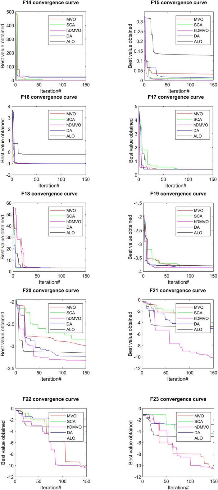
Convergence curves of MVO, SCA, ALO, DA, and hDMVO variants for composite functions.
Medium-scale instances of DTCTP
The medium-scale instances include two 63-activity problems wherein each activity has maximum five modes22. The network diagram of this problem is shown in Fig. 10. The time–cost alternatives for these instances are listed in Table 8. The medium-scale instances, including 1.37 × 1042 possible solutions will be tested at two different levels of indirect costs. The indirect cost in the first problem (63a) is 2300USD/day, while that in the second problem (63b) is 3500USD/day. The optimal solutions for these two problems are 5,421,120USD and 6,176,170USD, respectively. The hDMVO algorithm has been implemented in Python and is compatible with Visual Studio Code. The testing of all instances of DTCTP were performed on a personal computer featuring an Intel Core i7-8750H 2.20 GHz CPU and 8.0 GB of RAM.
Figure 10.
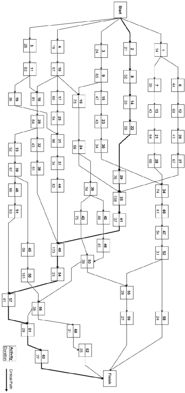
Activity on the node (AoN) representation of the 63-activity network (Aminbakhsh and Sonmez20).
Table 8.
Data for the 63 activity time–cost trade-off problem.
| Action | Pred | Dur1 | Cost1 | Dur2 | Cost2 | Dur3 | Cost3 | Dur4 | Cost4 | Dur5 | Cost5 |
|---|---|---|---|---|---|---|---|---|---|---|---|
| 1 | – | 14 | 3750 | 12 | 4250 | 10 | 5400 | 9 | 6250 | – | – |
| 2 | – | 21 | 11,250 | 18 | 14,800 | 17 | 16,200 | 15 | 19,650 | – | – |
| 3 | – | 24 | 22,450 | 22 | 24,900 | 19 | 27,950 | 17 | 31,650 | – | – |
| 4 | – | 19 | 17,800 | 17 | 19,400 | 15 | 21,600 | – | – | – | – |
| 5 | – | 28 | 31,180 | 26 | 34,200 | 23 | 38,250 | 21 | 41,400 | – | – |
| 6 | 1 | 44 | 54,260 | 42 | 58,450 | 38 | 63,225 | 35 | 68,150 | – | – |
| 7 | 1 | 39 | 47,600 | 36 | 50,750 | 33 | 54,800 | 30 | 59,750 | – | – |
| 8 | 2 | 52 | 62,140 | 47 | 69,700 | 44 | 72,600 | 39 | 81,750 | – | – |
| 9 | 3 | 63 | 72,750 | 59 | 79,450 | 55 | 86,250 | 51 | 91,500 | 49 | 99,500 |
| 10 | 4 | 57 | 66,500 | 53 | 70,250 | 50 | 75,800 | 46 | 80,750 | 41 | 86,450 |
| 11 | 5 | 63 | 83,100 | 59 | 89,450 | 55 | 97,800 | 50 | 104,250 | 45 | 112,400 |
| 12 | 6 | 68 | 75,500 | 62 | 82,000 | 58 | 87,500 | 53 | 91,800 | 49 | 96,550 |
| 13 | 7 | 40 | 34,250 | 37 | 38,500 | 33 | 43,950 | 31 | 48,750 | – | – |
| 14 | 8 | 33 | 52,750 | 30 | 58,450 | 27 | 63,400 | 25 | 66,250 | – | – |
| 15 | 9 | 47 | 38,140 | 40 | 41,500 | 35 | 47,650 | 32 | 54,100 | – | – |
| 16 | 9,10 | 75 | 94,600 | 70 | 101,250 | 66 | 112,750 | 61 | 124,500 | 57 | 132,850 |
| 17 | 10 | 60 | 78,450 | 55 | 84,500 | 49 | 91,250 | 47 | 94,640 | – | – |
| 18 | 10,11 | 81 | 127,150 | 73 | 143,250 | 66 | 154,600 | 61 | 161,900 | – | – |
| 19 | 11 | 36 | 82,500 | 34 | 94,800 | 30 | 101,700 | – | – | – | – |
| 20 | 12 | 41 | 48,350 | 37 | 53,250 | 34 | 59,450 | 32 | 66,800 | – | – |
| 21 | 13 | 64 | 85,250 | 60 | 92,600 | 57 | 99,800 | 53 | 107,500 | 49 | 113,750 |
| 22 | 14 | 58 | 74,250 | 53 | 79,100 | 50 | 86,700 | 47 | 91,500 | 42 | 97,400 |
| 23 | 15 | 43 | 66,450 | 41 | 69,800 | 37 | 75,800 | 33 | 81,400 | 30 | 88,450 |
| 24 | 16 | 66 | 72,500 | 62 | 78,500 | 58 | 83,700 | 53 | 89,350 | 49 | 96,400 |
| 25 | 17 | 54 | 66,650 | 50 | 70,100 | 47 | 74,800 | 43 | 79,500 | 40 | 86,800 |
| 26 | 18 | 84 | 93,500 | 79 | 102,500 | 73 | 111,250 | 68 | 119,750 | 62 | 128,500 |
| 27 | 20 | 67 | 78,500 | 60 | 86,450 | 57 | 89,100 | 56 | 91,500 | 53 | 94,750 |
| 28 | 21 | 66 | 85,000 | 63 | 89,750 | 60 | 92,500 | 58 | 96,800 | 54 | 100,500 |
| 29 | 22 | 76 | 92,700 | 71 | 98,500 | 67 | 104,600 | 64 | 109,900 | 60 | 115,600 |
| 30 | 23 | 34 | 27,500 | 32 | 29,800 | 29 | 31,750 | 27 | 33,800 | 26 | 36,200 |
| 31 | 19,25 | 96 | 145,000 | 89 | 154,800 | 83 | 168,650 | 77 | 179,500 | 72 | 189,100 |
| 32 | 26 | 43 | 43,150 | 40 | 48,300 | 37 | 51,450 | 35 | 54,600 | 33 | 61,450 |
| 33 | 26 | 52 | 61,250 | 49 | 64,350 | 44 | 68,750 | 41 | 74,500 | 38 | 79,500 |
| 34 | 28,30 | 74 | 89,250 | 71 | 93,800 | 66 | 99,750 | 62 | 105,100 | 57 | 114,250 |
| 35 | 24,27,29 | 138 | 183,000 | 126 | 201,500 | 115 | 238,000 | 103 | 283,750 | 98 | 297,500 |
| 36 | 24 | 54 | 47,500 | 49 | 50,750 | 42 | 56,800 | 38 | 62,750 | 33 | 68,250 |
| 37 | 31 | 34 | 22,500 | 32 | 24,100 | 29 | 26,750 | 27 | 29,800 | 24 | 31,600 |
| 38 | 32 | 51 | 61,250 | 47 | 65,800 | 44 | 71,250 | 41 | 76,500 | 38 | 80,400 |
| 39 | 33 | 67 | 81,150 | 61 | 87,600 | 57 | 92,100 | 52 | 97,450 | 49 | 102,800 |
| 40 | 34 | 41 | 45,250 | 39 | 48,400 | 36 | 51,200 | 33 | 54,700 | 31 | 58,200 |
| 41 | 35 | 37 | 17,500 | 31 | 21,200 | 27 | 26,850 | 23 | 32,300 | – | – |
| 42 | 36 | 44 | 36,400 | 41 | 39,750 | 38 | 42,800 | 32 | 48,300 | 30 | 50,250 |
| 43 | 36 | 75 | 66,800 | 69 | 71,200 | 63 | 76,400 | 59 | 81,300 | 54 | 86,200 |
| 44 | 37 | 82 | 102,750 | 76 | 109,500 | 70 | 127,000 | 66 | 136,800 | 63 | 146,000 |
| 45 | 39 | 59 | 84,750 | 55 | 91,400 | 51 | 101,300 | 47 | 126,500 | 43 | 142,750 |
| 46 | 39 | 66 | 94,250 | 63 | 99,500 | 59 | 108,250 | 55 | 118,500 | 50 | 136,000 |
| 47 | 40 | 54 | 73,500 | 51 | 78,500 | 47 | 83,600 | 44 | 88,700 | 41 | 93,400 |
| 48 | 42 | 41 | 36,750 | 39 | 39,800 | 37 | 43,800 | 34 | 48,500 | 31 | 53,950 |
| 49 | 38,41,44 | 173 | 267,500 | 159 | 289,700 | 147 | 312,000 | 138 | 352,500 | 121 | 397,750 |
| 50 | 45 | 101 | 47,800 | 74 | 61,300 | 63 | 76,800 | 49 | 91,500 | – | – |
| 51 | 46 | 83 | 84,600 | 77 | 93,650 | 72 | 98,500 | 65 | 104,600 | 61 | 113,200 |
| 52 | 47 | 31 | 23,150 | 28 | 27,600 | 26 | 29,800 | 24 | 32,750 | 21 | 35,200 |
| 53 | 43,48 | 39 | 31,500 | 36 | 34,250 | 33 | 37,800 | 29 | 41,250 | 26 | 44,600 |
| 54 | 49 | 23 | 16,500 | 22 | 17,800 | 21 | 19,750 | 20 | 21,200 | 18 | 24,300 |
| 55 | 52,53 | 29 | 23,400 | 27 | 25,250 | 26 | 26,900 | 24 | 29,400 | 22 | 32,500 |
| 56 | 50,53 | 38 | 41,250 | 35 | 44,650 | 33 | 47,800 | 31 | 51,400 | 29 | 55,450 |
| 57 | 51,54 | 41 | 37,800 | 38 | 41,250 | 35 | 45,600 | 32 | 49,750 | 30 | 53,400 |
| 58 | 52 | 24 | 12,500 | 22 | 13,600 | 20 | 15,250 | 18 | 16,800 | 16 | 19,450 |
| 59 | 55 | 27 | 34,600 | 24 | 37,500 | 22 | 41,250 | 19 | 46,750 | 17 | 50,750 |
| 60 | 56 | 31 | 28,500 | 29 | 30,500 | 27 | 33,250 | 25 | 38,000 | 21 | 43,800 |
| 61 | 56,57 | 29 | 22,500 | 27 | 24,750 | 25 | 27,250 | 22 | 29,800 | 20 | 33,500 |
| 62 | 60 | 25 | 38,750 | 23 | 41,200 | 21 | 44,750 | 19 | 49,800 | 17 | 51,100 |
| 63 | 61 | 27 | 9500 | 26 | 9700 | 25 | 10,100 | 24 | 10,800 | 22 | 12,700 |
hDMVO obtains exceptional results in medium-scale experimental problems, wherein the best values among the ten runs are 5,444,670USD for problems 63a (Table 9) and 6,211,720USD for problems 63b (Table 10). The distribution of percentage deviations for hDMVO, MVO, and SCA are illustrated in Figs. 11 and 12, using ten trials of the 63a and 63b DTCTP problems. The figures demonstrate that hDMVO has a smaller deviation percentage compared to MVO and SCA, indicating its ability to effectively balance exploration and exploitation when solving medium-scale DTCTP problems.
Table 9.
Analysis results of problem 63a.
| No | SCA | MVO | hDMVO | |||
|---|---|---|---|---|---|---|
| Dur | Cost | Dur | Cost | Dur | Cost | |
| 1 | 656 | 5,747,490 | 635 | 5,475,030 | 632 | 5,444,670 |
| 2 | 631 | 5,748,170 | 629 | 5,475,980 | 638 | 5,445,380 |
| 3 | 626 | 5,761,900 | 637 | 5,476,980 | 635 | 5,453,820 |
| 4 | 638 | 5,772,130 | 631 | 5,477,170 | 626 | 5,455,050 |
| 5 | 638 | 5,772,330 | 612 | 5,478,790 | 635 | 5,455,620 |
| 6 | 650 | 5,775,665 | 636 | 5,478,930 | 629 | 5,456,190 |
| 7 | 632 | 5,783,255 | 636 | 5,479,820 | 636 | 5,457,050 |
| 8 | 652 | 5,788,430 | 633 | 5,480,820 | 630 | 5,457,270 |
| 9 | 628 | 5,798,400 | 632 | 5,481,190 | 632 | 5,458,260 |
| 10 | 629 | 5,820,580 | 630 | 5,481,280 | 651 | 5,459,130 |
| Pop. size | 200 | 200 | 200 | |||
| Num. of iterations | 250 | 250 | 250 | |||
| Num. of function evaluation | 50,000 | 50,000 | 50,000 | |||
Table 10.
Analysis results of problem 63b.
| No | SCA | MVO | hDMVO | |||
|---|---|---|---|---|---|---|
| Dur | Cost | Dur | Cost | Dur | Cost | |
| 1 | 628 | 6,524,960 | 596 | 6,252,550 | 626 | 6,211,720 |
| 2 | 623 | 6,515,560 | 621 | 6,252,790 | 592 | 6,213,340 |
| 3 | 607 | 6,507,315 | 602 | 6,253,410 | 613 | 6,214,290 |
| 4 | 601 | 6,534,900 | 595 | 6,254,850 | 613 | 6,216,270 |
| 5 | 602 | 6,525,940 | 626 | 6,255,250 | 618 | 6,219,720 |
| 6 | 588 | 6,510,775 | 623 | 6,255,420 | 614 | 6,219,780 |
| 7 | 618 | 6,532,965 | 586 | 6,256,265 | 623 | 6,223,840 |
| 8 | 614 | 6,567,555 | 598 | 6,256,440 | 621 | 6,224,580 |
| 9 | 617 | 6,503,725 | 602 | 6,256,790 | 590 | 6,225,290 |
| 10 | 571 | 6,575,900 | 627 | 6,257,390 | 619 | 6,229,130 |
| Pop. size | 200 | 200 | 200 | |||
| Num. of iterations | 250 | 250 | 250 | |||
| Num. of function evaluation | 50,000 | 50,000 | 50,000 | |||
Figure 11.
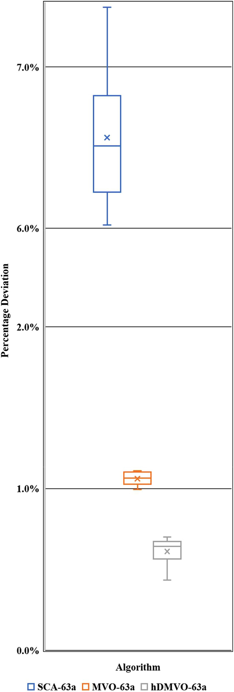
Percentage deviations of hDMVO, MVO and SCA in problem 63a.
Figure 12.
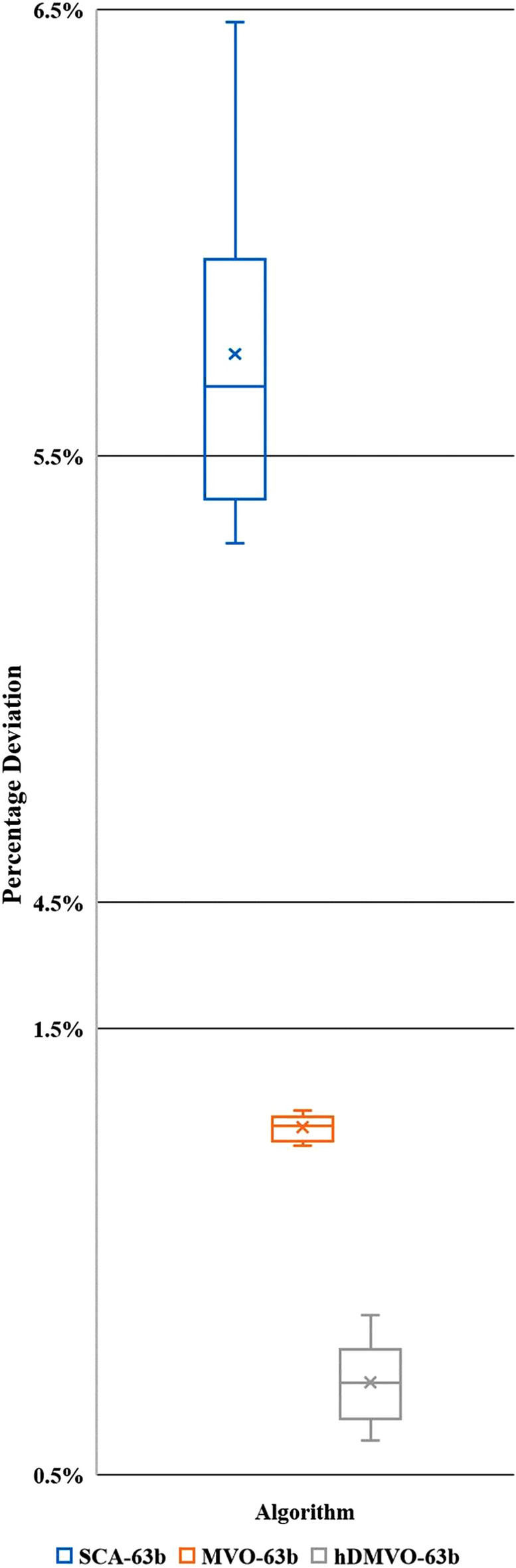
Percentage deviations of hDMVO, MVO and SCA in problem 63b.
The average percent deviation (APD) of hDMVO from the global optimal for problems 63a and 63b is summarized in Table 11. The results show that hDMVO outperforms ACO, GA, and electromagnetism mechanism (EMS)18, sole genetic algorithm (GA), hybrid genetic algorithm (HA)22, modified adaptive weight approach with genetic algorithms (MAWA-GA), modified adaptive weight approach with particle swarm optimization (MAWA-PSO) and modified adaptive weight approach with teaching learning based optimization (MAWA-TLBO)37. hDMVO also outperforms the two original algorithms named MVO and SCA when its ADPs are 0.61% and 0.71% for problems 63a and 63b, respectively, within 50,000 schedules. As evident from Table 11, hDMVO outperforms both native algorithms (MVO and SCA) in medium-scale instances. By searching only 50,000 solutions out of 1.37 × 1042 potential solutions, hDMVO can identify high-quality solutions that were highly close to the optimal value.
Table 11.
Average percent deviation from the optimal for problem 63a and 63b.
| Algorithm | 63a | 63b | ||
|---|---|---|---|---|
| No. of runs | APD (%) | No. of runs | APD (%) | |
| ACO (Bettemir18) | 10 | 1.30 | 10 | 0.80 |
| EMS (Bettemir18) | 10 | 2.13 | 10 | 2.40 |
| GA (Bettemir18) | 10 | 5.19 | 10 | 4.27 |
| GA (Sonmez and Bettemir22) | 10 | 5.86 | 10 | 5.16 |
| HA (Sonmez and Bettemir22) | 10 | 2.61 | 10 | 2.50 |
| MAWA-GA (Toğan and Eirgash37) | 10 | 7.01 | 10 | 4.07 |
| MAWA-PSO (Toğan and Eirgash37) | 10 | 8.38 | 10 | 7.72 |
| MAWA-TLBO (Toğan and Eirgash37) | 10 | 3.62 | 10 | 1.63 |
| SCA (This study) | 10 | 6.56 | 10 | 5.73 |
| MVO (This study) | 10 | 1.06 | 10 | 1.28 |
| hDMVO (This study) | 10 | 0.61 | 10 | 0.71 |
Large-scale instances of DTCTP
The large-scale instances include two 630-activity problems, wherein each activity has a maximum of five modes, including 2.38 × 10421 possible solutions22. These cases represent the size of an actual construction project. The indirect costs for large-scale instances (630a and 630b) are similar to those of medium-scale instances (2300USD/day and 3500USD/day for 63a and 63b, respectively).
The hDMVO algorithm also shows its effectiveness in large-scale experimental problems; the best values for ten runs in problems 630a and 630b are 54,816,950USD (Table 12) and 62,505,580USD (Table 13), respectively. Figures 13 and 14 show the boxplots of ten percentage deviations of hDMVO, MVO and SCA by testing problems 630a and 630b. From Figs. 13 and 14, the percentage deviations of hDMVO are much smaller than those of MVO and SCA. The results thus demonstrated the stability of hDMVO when solving the large-scale DTCTP problem.
Table 12.
Analysis results of problem 630a.
| No | SCA | MVO | hDMVO | |||
|---|---|---|---|---|---|---|
| Dur | Cost | Dur | Cost | Dur | Cost | |
| 1 | 5654 | 59,911,250 | 6323 | 55,080,630 | 6317 | 54,816,950 |
| 2 | 5628 | 59,980,560 | 6291 | 55,082,810 | 6306 | 54,820,585 |
| 3 | 5615 | 60,000,610 | 6322 | 55,099,890 | 6330 | 54,849,050 |
| 4 | 5612 | 60,019,530 | 6296 | 55,110,705 | 6300 | 54,883,485 |
| 5 | 5641 | 60,082,860 | 6295 | 55,111,040 | 6324 | 54,897,700 |
| 6 | 5613 | 60,141,055 | 6270 | 55,122,000 | 6311 | 54,924,330 |
| 7 | 5632 | 60,165,040 | 6273 | 55,122,360 | 6322 | 54,937,240 |
| 8 | 5631 | 60,196,945 | 6281 | 55,135,870 | 6339 | 54,949,000 |
| 9 | 5612 | 60,197,985 | 6313 | 55,190,530 | 6355 | 54,951,200 |
| 10 | 5586 | 60,240,730 | 6334 | 55,199,825 | 6291 | 54,993,930 |
| Pop. size | 200 | 200 | 200 | |||
| Num. of iterations | 250 | 250 | 250 | |||
| Num. of function evaluation | 50,000 | 50,000 | 50,000 | |||
Table 13.
Analysis results of problem 630b.
| No | SCA | MVO | hDMVO | |||
|---|---|---|---|---|---|---|
| Dur | Cost | Dur | Cost | Dur | Cost | |
| 1 | 5604 | 66,647,315 | 6052 | 62,742,405 | 6097 | 62,505,580 |
| 2 | 5592 | 66,676,865 | 6088 | 62,759,350 | 5991 | 62,526,385 |
| 3 | 5587 | 66,712,740 | 5997 | 62,763,350 | 6020 | 62,537,900 |
| 4 | 5597 | 66,924,805 | 6027 | 62,783,920 | 6117 | 62,538,830 |
| 5 | 5583 | 66,961,860 | 6064 | 62,798,565 | 6042 | 62,544,040 |
| 6 | 5632 | 66,975,580 | 6027 | 62,815,320 | 6056 | 62,544,470 |
| 7 | 5642 | 66,985,310 | 6016 | 62,827,245 | 6105 | 62,561,260 |
| 8 | 5604 | 67,006,655 | 6036 | 62,839,590 | 6015 | 62,570,390 |
| 9 | 5599 | 67,026,155 | 5985 | 62,843,840 | 5998 | 62,588,460 |
| 10 | 5609 | 67,092,830 | 6097 | 62,863,315 | 6060 | 62,591,215 |
| Pop. size | 200 | 200 | 200 | |||
| Num. of iterations | 250 | 250 | 250 | |||
| Num. of function evaluation | 50,000 | 50,000 | 50,000 | |||
Figure 13.
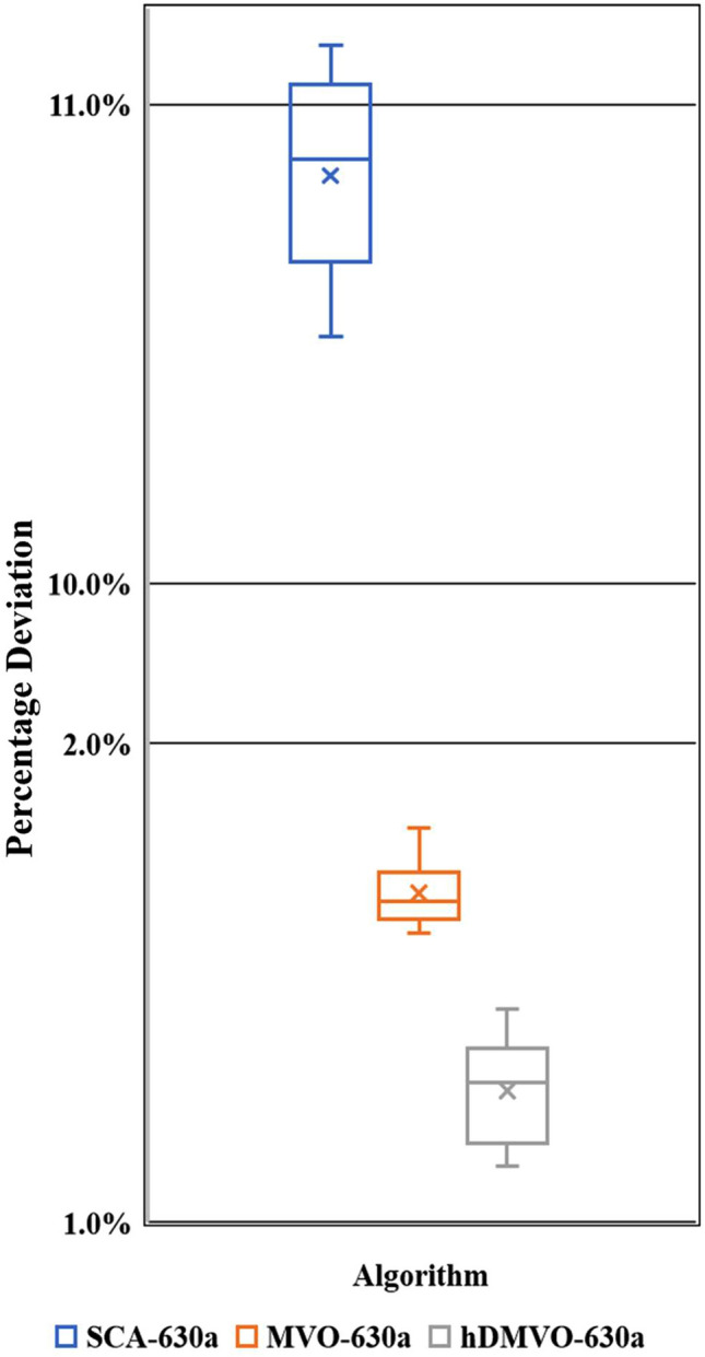
Percentage deviations of hDMVO, MVO and SCA in problem 630a.
Figure 14.
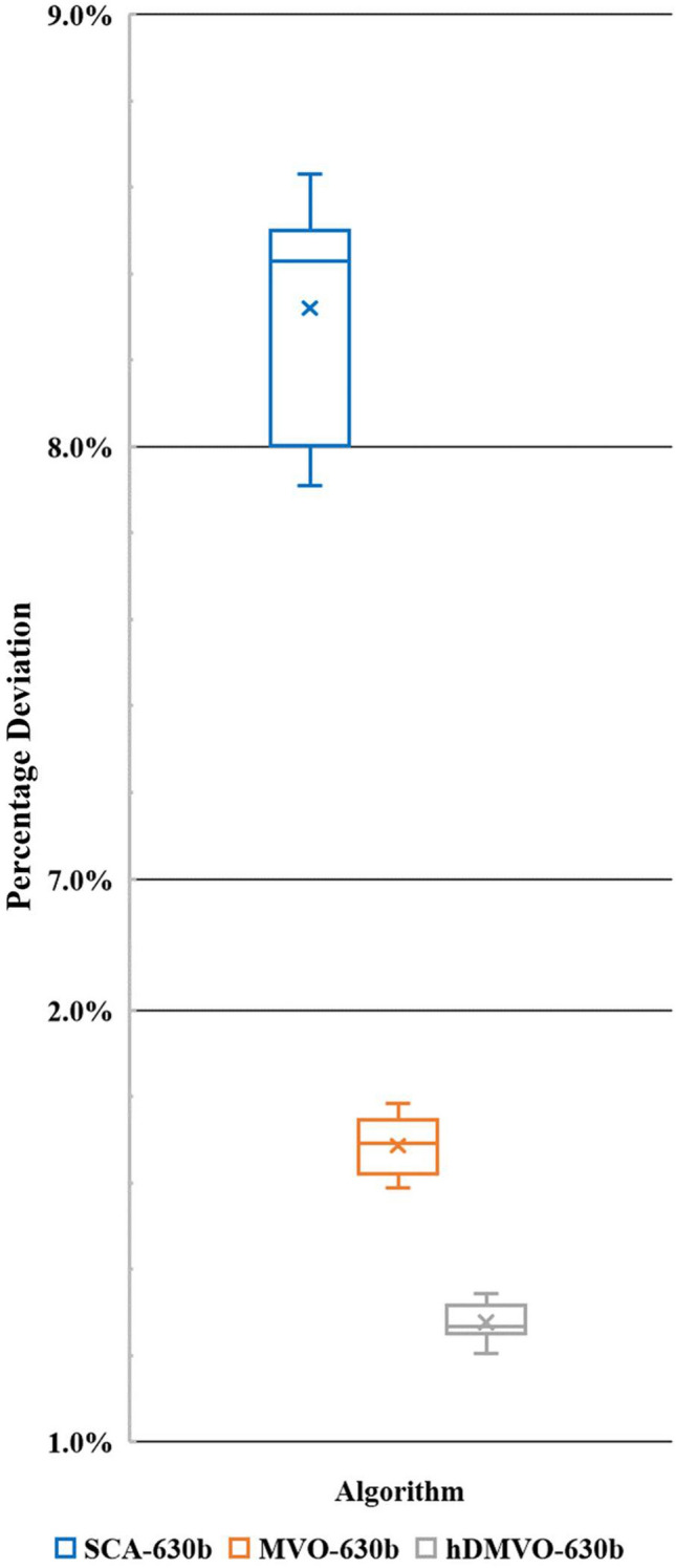
Percentage deviations of hDMVO, MVO and SCA in problem 630b.
For large-scale instances, hDMVO provides superior results (Table 14) against GA, genetic algorithm with simulated annealing (GASA), hybrid genetic algorithm with quantum simulated annealing (HGAQSA), genetic memetic algorithm with simulated annealing (GMASA), genetic algorithm with simulated annealing and variable neighborhood search (GASAVNS), PSO, electromagnetic scatter search (ESS)18, and GA and HA22. hDMVO completely outperforms SCA and performs slightly better than MVO. hDMVO also yields better results than NDS–TLBO30 in problem 630b; for problem 630a, hDMVO achieves APD of 1.27% when searching for 50,000 solutions, while NDS–TLBO achieves APD of 1.1% when searching for 250,000 solutions. hDMVO's ADP values for problems 630a and 630b are 1.27% and 1.28%, respectively (Table 8), which were significantly superior to those of the two original algorithms, MVO and SCA. By just searching for 50,000 solutions out of 2.38 × 10421 potential solutions, hDMVO can achieve high-quality solutions for large-scale instances. These results indicate that hDMVO has overcome the disadvantages of MVO and SCA in search space exploration and exploitation to achieve the optimal value.
Table 14.
Average percent deviation from the optimal for problem 630a and 630b.
| Algorithm | 630a | 630b | ||
|---|---|---|---|---|
| No. of runs | APD (%) | No. of runs | APD (%) | |
| GA (Bettemir18) | 10 | 8.83 | 10 | 7.50 |
| GASA (Bettemir18) | 10 | 8.84 | 10 | 7.59 |
| HGAQSA (Bettemir18) | 10 | 2.41 | 10 | 2.47 |
| GMASA (Bettemir18) | 10 | 8.02 | 10 | 7.56 |
| GASAVNS (Bettemir18) | 10 | 7.97 | 10 | 7.38 |
| PSO (Bettemir18) | 10 | 1.12 | 10 | 2.20 |
| ACO (Bettemir18) | 10 | 4.95 | 10 | 4.56 |
| ESS (Bettemir18) | 10 | 8.86 | 10 | 7.70 |
| GA (Sonmez and Bettemir22) | 10 | 8.83 | 10 | 7.50 |
| HA (Sonmez and Bettemir 22) | 10 | 2.41 | 10 | 2.47 |
| NDS-TLBO (Eirgash, Toğan et al.30) | 10 | 1.1 | 10 | 1.51 |
| SCA (This study) | 10 | 10.85 | 10 | 8.32 |
| MVO (This study) | 10 | 1.69 | 10 | 1.69 |
| hDMVO (This study) | 10 | 1.27 | 10 | 1.28 |
Conclusion
This study presents a combined model of MVO and SCA for global optimization. The combination's objective is to make use of the exploration of MVO and the search space exploitation of SCA to achieve an effective balance between the two phases during optimization. hDMVO is developed to combine the search space exploitation mechanism of MVO and SCA while preserving MVO's mechanisms of roulette wheel selection, thereby improving hDMVO's search exploration and exploitation. hDMVO was comprehensively evaluated by twenty-three benchmark optimization problems. The results indicate that hDMVO is more likely to achieve global optimization compared with SCA and MVO. In this study, hDMVO is proposed to solve the discrete time–cost trade-off problem in construction projects. The results of the computational experiments reveal that hDMVO can achieve high-quality solutions for medium- and large-scale DTCTP and can be used to optimize the cost–time problems for actual projects. With the obtained results, hDMVO is seen as an appropriate metaheuristic method for solving the DTCTP problem as well as other optimization problems.
Recommendations for future work
In this study, the application of hDMVO is limited to solving DTCTP problems with the finish-to-start relationship. However, in actual construction projects, DTCTP problems in construction projects often include the start-to-start, finish-to-finish, and start-to-finish relationships. Therefore, in future studies, hDMVO will be used to solve DTCTP problems with complicated relationships simultaneously and on a large scale to obtain more comprehensive solutions for project management. The hDMVO model has been shown to effectively balance exploration and exploitation when compared to other state-of-the-art swarm-based optimization algorithms (DA, ALO, SCA, and MVO). Additionally, the hDMVO model also demonstrates competitive performance in medium- and large-scale DTCTPs. However, limitations in local optima avoidance are also clearly demonstrated by hDMVO when applied to large-scale problems. To overcome these limitations, future research will involve the development of a combination model that incorporates hDMVO with other techniques such as modified adaptive weight approach and opposition-based learning, to enhance its performance in solving optimization problems in the construction industry and other technical fields.
Acknowledgements
We would like to thank Ho Chi Minh City University of Technology (HCMUT), VNU-HCM for the support of time and facilities for this study.
Author contributions
Both P.V.H.S. and N.D.N.T. wrote all the main manuscript, prepared all the figures, tables and checked revision before submission.
Funding
The authors whose names are listed immediately below certify that they have NO affiliations with or involvement in any organization or entity with any financial interest (such as honoraria; educational grants; participation in speakers’ bureaus; membership, employment, consultancies, stock ownership, or other equity interest; and expert testimony or patent-licensing arrangements), or non-financial interest (such as personal or professional relationships, affiliations, knowledge or beliefs) in the subject matter or materials discussed in this manuscript.
Data availability
Some or all data, models, or code that support the findings of this study are available from the corresponding author upon reasonable request.
Competing interests
The authors declare no competing interests.
Footnotes
Publisher's note
Springer Nature remains neutral with regard to jurisdictional claims in published maps and institutional affiliations.
References
- 1.Vanhoucke M, Debels D. The discrete time/cost trade-off problem: Extensions and heuristic procedures. J. Sched. 2007;10(4):311–326. doi: 10.1007/s10951-007-0031-y. [DOI] [Google Scholar]
- 2.Mirjalili S, Mirjalili SM, Hatamlou A. Multi-verse optimizer: A nature-inspired algorithm for global optimization. Neural Comput. Appl. 2016;27(2):495–513. doi: 10.1007/s00521-015-1870-7. [DOI] [Google Scholar]
- 3.Laith A. Multi-verse optimizer algorithm: A comprehensive survey of its results, variants, and applications. Neural Comput. Appl. 2020;32(16):12381–12401. doi: 10.1007/s00521-020-04839-1. [DOI] [Google Scholar]
- 4.Mirjalili S. SCA: a sine cosine algorithm for solving optimization problems. Knowl. Based Syst. 2016;96:120–133. doi: 10.1016/j.knosys.2015.12.022. [DOI] [Google Scholar]
- 5.Rizk-Allah RM, Hassanien AE. A comprehensive survey on the sine–cosine optimization algorithm. Artif. Intell. Rev. 2022 doi: 10.1007/s10462-022-10277-3. [DOI] [Google Scholar]
- 6.Abualigah L, Diabat A. Advances in sine cosine algorithm: A comprehensive survey. Artif. Intell. Rev. 2021;54(4):2567–2608. doi: 10.1007/s10462-020-09909-3. [DOI] [PMC free article] [PubMed] [Google Scholar]
- 7.Parejo JA, et al. Metaheuristic optimization frameworks: A survey and benchmarking. Soft. Comput. 2012;16(3):527–561. doi: 10.1007/s00500-011-0754-8. [DOI] [Google Scholar]
- 8.Zhou A, et al. Multiobjective evolutionary algorithms: A survey of the state of the art. Swarm Evol. Comput. 2011;1(1):32–49. doi: 10.1016/j.swevo.2011.03.001. [DOI] [Google Scholar]
- 9.Mirjalili S. Dragonfly algorithm: A new meta-heuristic optimization technique for solving single-objective, discrete, and multi-objective problems. Neural Comput. Appl. 2016;27(4):1053–1073. doi: 10.1007/s00521-015-1920-1. [DOI] [Google Scholar]
- 10.Son PVH, Khoi TT. Development of Africa Wild Dog optimization algorithm for optimize freight coordination for decreasing greenhouse gases. In: Reddy JN, Wang CM, Luong VH, Le AT, editors. ICSCEA 2019. Springer; 2020. pp. 881–889. [Google Scholar]
- 11.Holland JH. Adaptation in Natural and Artificial Systems: An Introductory Analysis with Applications to Biology, Control, and Artificial Intelligence. MIT Press; 1992. [Google Scholar]
- 12.Wolpert DH, Macready WG. No free lunch theorems for optimization. IEEE Trans. Evol. Comput. 1997;1(1):67–82. doi: 10.1109/4235.585893. [DOI] [Google Scholar]
- 13.Zhang Y, Thomas Ng S. An ant colony system based decision support system for construction time-cost optimization. J. Civ. Eng. Manag. 2012;18(4):580–589. doi: 10.3846/13923730.2012.704164. [DOI] [Google Scholar]
- 14.Son PVH, Duy NHC, Dat PT. Optimization of construction material cost through logistics planning model of dragonfly algorithm—Particle swarm optimization. KSCE J. Civ. Eng. 2021;25(7):2350–2359. doi: 10.1007/s12205-021-1427-5. [DOI] [Google Scholar]
- 15.Rizk-Allah RM. A quantum-based sine cosine algorithm for solving general systems of nonlinear equations. Artif. Intell. Rev. 2021;54(5):3939–3990. doi: 10.1007/s10462-020-09944-0. [DOI] [Google Scholar]
- 16.Rizk-Allah RM. An improved sine–cosine algorithm based on orthogonal parallel information for global optimization. Soft. Comput. 2019;23(16):7135–7161. doi: 10.1007/s00500-018-3355-y. [DOI] [Google Scholar]
- 17.Rizk-Allah RM. Hybridizing sine cosine algorithm with multi-orthogonal search strategy for engineering design problems. J. Comput. Des. Eng. 2018;5(2):249–273. [Google Scholar]
- 18.Bettemir, Ö. H. Optimization of Time-Cost-Resource Trade-Off Problems in Project Scheduling Using Meta-Heuristic Algorithms (2009).
- 19.Zhang H, Xing F. Fuzzy-multi-objective particle swarm optimization for time–cost–quality tradeoff in construction. Autom. Constr. 2010;19(8):1067–1075. doi: 10.1016/j.autcon.2010.07.014. [DOI] [Google Scholar]
- 20.Aminbakhsh S, Sonmez R. Discrete particle swarm optimization method for the large-scale discrete time–cost trade-off problem. Expert Syst. Appl. 2016;51:177–185. doi: 10.1016/j.eswa.2015.12.041. [DOI] [Google Scholar]
- 21.Aminbakhsh S, Sonmez R. Pareto front particle swarm optimizer for discrete time-cost trade-off problem. J. Comput. Civ. Eng. 2017;31(1):04016040. doi: 10.1061/(ASCE)CP.1943-5487.0000606. [DOI] [Google Scholar]
- 22.Sonmez R, Bettemir ÖH. A hybrid genetic algorithm for the discrete time–cost trade-off problem. Expert Syst. Appl. 2012;39(13):11428–11434. doi: 10.1016/j.eswa.2012.04.019. [DOI] [Google Scholar]
- 23.Zhang L, Zou X, Qi J. A trade-off between time and cost in scheduling repetitive construction projects. J. Ind. Manag. Optim. 2015;11(4):1423. doi: 10.3934/jimo.2015.11.1423. [DOI] [Google Scholar]
- 24.Naseri H, Ghasbeh MAE. Time-cost trade off to compensate delay of project using genetic algorithm and linear programming. Int. J. Innov. Manag. Technol. 2018;9(6):285–290. doi: 10.18178/ijimt.2018.9.6.826. [DOI] [Google Scholar]
- 25.Bettemir ÖH, Talat Birgönül M. Network analysis algorithm for the solution of discrete time-cost trade-off problem. KSCE J. Civ. Eng. 2017;21(4):1047–1058. doi: 10.1007/s12205-016-1615-x. [DOI] [Google Scholar]
- 26.Son PVH, Khoi LNQ. Utilizing artificial intelligence to solving time–cost–quality trade-off problem. Sci. Rep. 2022;12(1):20112. doi: 10.1038/s41598-022-24668-7. [DOI] [PMC free article] [PubMed] [Google Scholar]
- 27.Zheng, H. Multi-mode discrete time-cost-environment trade-off problem of construction systems for large-scale hydroelectric projects. in Proceedings of the Ninth International Conference on Management Science and Engineering Management (Springer, 2015).
- 28.Said SS, Haouari M. A hybrid simulation-optimization approach for the robust discrete time/cost trade-off Problem. Appl. Math. Comput. 2015;259:628–636. [Google Scholar]
- 29.Tran D-H, et al. Opposition multiple objective symbiotic organisms search (OMOSOS) for time, cost, quality and work continuity tradeoff in repetitive projects. J. Comput. Des. Eng. 2018;5(2):160–172. [Google Scholar]
- 30.Eirgash MA, Toğan V, Dede T. A multi-objective decision making model based on TLBO for the time-cost trade-off problems. Struct. Eng. Mech. 2019;71(2):139–151. [Google Scholar]
- 31.Alavipour SR, Arditi D. Time-cost tradeoff analysis with minimized project financing cost. Autom. Constr. 2019;98:110–121. doi: 10.1016/j.autcon.2018.09.009. [DOI] [Google Scholar]
- 32.Albayrak G. Novel hybrid method in time–cost trade-off for resource-constrained construction projects. Iran. J. Sci. Technol. Trans. Civ. Eng. 2020;44(4):1295–1307. doi: 10.1007/s40996-020-00437-2. [DOI] [Google Scholar]
- 33.Sharma K, Trivedi MK. Latin hypercube sampling-based NSGA-III optimization model for multimode resource constrained time–cost–quality–safety trade-off in construction projects. Int. J. Constr. Manag. 2020;22(16):3158–3168. [Google Scholar]
- 34.Li X, et al. Multimode time-cost-robustness trade-off project scheduling problem under uncertainty. J. Comb. Optim. 2020;43(5):1173–1202. doi: 10.1007/s10878-020-00636-7. [DOI] [Google Scholar]
- 35.De P, et al. The discrete time-cost tradeoff problem revisited. Eur. J. Oper. Res. 1995;81(2):225–238. doi: 10.1016/0377-2217(94)00187-H. [DOI] [Google Scholar]
- 36.Črepinšek M, Liu S-H, Mernik M. Exploration and exploitation in evolutionary algorithms: A survey. ACM Comput. Surv. (CSUR) 2013;45(3):1–33. doi: 10.1145/2480741.2480752. [DOI] [Google Scholar]
- 37.Toğan V, Eirgash MA. Time-cost trade-off optimization of construction projects using teaching learning based optimization. KSCE J. Civ. Eng. 2019;23(1):10–20. doi: 10.1007/s12205-018-1670-6. [DOI] [Google Scholar]
Associated Data
This section collects any data citations, data availability statements, or supplementary materials included in this article.
Data Availability Statement
Some or all data, models, or code that support the findings of this study are available from the corresponding author upon reasonable request.