Contrastive semi-supervised harmonization of single-shell to multi-shell diffusion MRI

Abstract

Diffusion weighted MRI (DW-MRI) harmonization is necessary for multi-site or multi-acquisition studies. Current statistical methods address the need to harmonize from one site to another, but do not simultaneously consider the use of multiple datasets which are comprised of multiple sites, acquisitions protocols, and age demographics. This work explores deep learning methods which can generalize across these variations through semi-supervised and unsupervised learning while also learning to estimate multi-shell data from single-shell data using the Multi-shell Diffusion MRI Harmonization Challenge (MUSHAC) and Baltimore Longitudinal Study on Aging (BLSA) datasets. We compare disentanglement harmonization models, which seek to encode anatomy and acquisition in separate latent spaces, and a CycleGAN harmonization model, which uses generative adversarial networks (GAN) to perform style transfer between sites, to the baseline preprocessing and to SHORE interpolation. We find that the disentanglement models achieve superior performance in harmonizing all data while at the same transforming the input data to a single target space across several diffusion metrics (fractional anisotropy, mean diffusivity, mean kurtosis, primary eigenvector).

INTRODUCTION

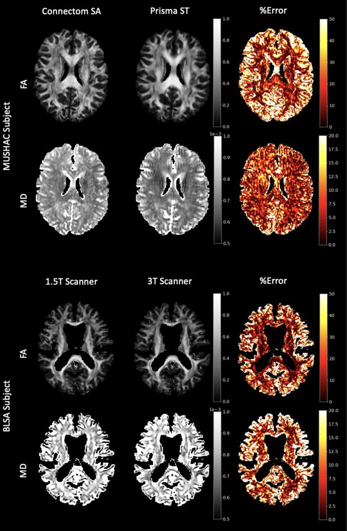
Diffusion weighted MRI (DW-MRI) is the only non-invasive modality to probe in vivo tissue microstructure and macrostructure [1]. DW-MRI has opened up new investigations into cognitive neuroscience and brain dysfunction in aging, mental health disorders, and neurological disease [2]. However, clinical adoption is hindered by the variability in DW-MRI measurements caused by differences in the number of head coils, coil sensitivity, imaging gradient non-linearities, magnetic field homogeneity, reconstruction algorithms, and software upgrades [3–7]. These differences are measured in terms of reproducibility across multiple acquisitions and across multiple sites (Figure 1), and the goal of increasing reproducibility across acquisition parameters, scanners, and scanning sites is known as harmonization.

Figure 1.

Hardware and protocol differences lead to reproducibility error in DW-MRI metrics. Examples of these differences are shown here for FA and MD for a subject from the MUSHAC dataset (top) as well as the BLSA dataset (bottom). Error is calculated as the absolute difference between metrics from two scans divided by the average of the two. While directly harmonizing between two sites is straightforward, it does not allow for multiple datasets each with multiple sites to be jointly analyzed as all sites would need to be moved to the same space.

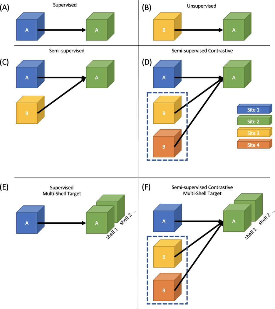
Many empirical models have been developed for the purpose of correcting hardware specific effects [8–12], but these rely on a particular set of acquisitions of acquisition parameters which may not be retroactively applied. A generalizable model would be desirable for already acquired datasets. DW-MRI harmonization has been approached using statistical methods such as ComBat [13] and Linear RISH [14] as well as deep learning approaches such as SHResNet [15] and StarGAN [16] (Table 1). These approaches fall under the category of supervised or unsupervised machine learning (Figure 2). However, supervised methods require matching subject scans at all sites, and unsupervised methods require a sufficient number of examples from each site and typically have poor performance when data have differing acquisition parameters. After testing 4 approaches, we propose a method which can harmonize data spanning multiple sites, acquisition parameters, age groups, and datasets using single-shell to multi-shell predictions [17] and semi-supervised contrastive learning [18]. We modify a harmonization method originally proposed for MRI contrast harmonization [19] and we rely on T1 derived segmentations as priors to our model. We compare these disentanglement approaches against a GAN approach to harmonization as well as standard preprocessing and SHORE as two baseline methods.

Table 1.

Statistical methods as well as deep learning methods all depend on b-value specific representations of DW-MRI. SHORE is a mutli-shell representation that is not dependent on the b-value and can be used to reconstruct any given acquisition scheme given a set of b-values and directions. We aim to create a deep learning framework which harmonizes across datasets without needing to match acquisition parameters across sites.

	Regression	Convolutional Neural Net	Supervised	Unsupervised	Semi-supervised	Semi-supervised Contrastive	Multi-shell Target
COMBAT [20]	✓	╳	╳	✓	╳	╳	╳
RISH [14]	✓	╳	╳	✓	╳	╳	╳
SHORE [24]	✓	╳	╳	╳	╳	╳	╳
SHResNet [15]	╳	✓	✓	╳	╳	╳	╳
StarGAN [16]	╳	✓	╳	✓	╳	╳	╳
NST [18]	╳	✓	╳	╳	╳	✓	╳
ShellDNN [17]	╳	✓	✓	╳	╳	╳	✓
This Work	╳	✓	╳	╳	╳	✓	✓

Figure 2.

Machine learning approaches in DW-MRI follow the general format of supervised (A) and unsupervised (B) methods. However, there are few approaches which follow the standard semi-supervised approach (C), but a contrastive approach which relies on having paired data across sites or acquisitions (D) has been shown to be effective. A problem more unique to DW-MRI is estimating a multi-shell acquisition from a single-shell acquisition (E). This work focuses on estimating a multi-shell target site from single-shell data in a semi-supervised contrastive learning framework (F).

FEATURES OF POPULAR HARMONIZATION METHODS

Statistical Models

Through analyzing the effectiveness of several statistical approaches that were developed for other data types, Fortin et al. [13] found that ComBat [20] achieved the best performance. Originally developed for genomics data, ComBat uses an empirical Bayes framework for adjusting data for batch effects that is robust to outliers in small sample sizes. A DTI harmonization technique proposed by Mirzaalian et al. [14] utilizes rotation invariant spherical harmonic (RISH) features and combines the unprocessed DTI images across scanners. A major drawback of these methods is that they require DTI data to have similar acquisition parameters which is often unfeasible in multi-site studies. Although, unlike supervised machine learning methods, acquisitions between sites do not need to be of the same subjects.

Deep Learning Models

Many deep learning approaches have been employed for diffusion harmonization as well. Nath et al. utilized a dual network to incorporate unlabeled paired in-vivo DW-MRI of human subjects along with labeled squirrel monkey DW-MRI with histology ground truth [18]. In a semi-supervised framework, this approach is analogous to utilizing a contrastive learning objective [21, 22] when a negative sample may not be sufficiently identified in the unlabeled data. In this work, the term contrastive is used to refer to this variation of the loss. Koppers et al. designed a residual network specifically for spherical harmonic representations of DW-MRI which predicts the spherical representation at one scanner given the spherical harmonics of another scanner [15]. Many of these methods are supervised and require matching subjects at all sites, and most of them rely on single-shell representations of the diffusion signal which would limit the models to acquisitions of similar b-values. However, previous work has used neural networks to estimate a second shell of a two shell acquisition given the first shell as input [17]. Given DW-MRI from multiple sources, Moyer et al. uses an unsupervised method based on variational auto-encoders to learn an intermediate representation that is invariant to site and protocol specific effects [16], and while this is free from the constraints of supervised learning, it ignores the use of matched subjects which can provide useful guidance to the model. Figure 2 generalizes the frameworks of these approaches and Table 1 summarizes the features of popular methods.

Deep learning approaches have been applied to harmonization in other modalities as well. For harmonization between T1 and T2 contrasts, Dewey et al. leverages paired T1 and T2 acquisitions to learn two latent spaces: one which encodes anatomical features and one which encodes acquisition features. The encoder is trained to generate the specified contrast using either sets of anatomical features [19]. CycleGAN has been used to learn style transfer between sites for MRI harmonization as well [23–25]. The cycle consistency loss in this framework ensures anatomical information is retained while the adversarial loss enforces the site-specific changes. In this work we explore the application of these methods for DW-MRI harmonization in a framework that allows for multiple datasets which are not limited by acquisition parameters.

DW-MRI Representations

Both statistical and deep learning approaches to DW-MRI harmonization typically rely on single-shell representations of the signal. SH and RISH represent the data in comparatively few features when considering the number of diffusion volumes acquired in most acquisitions. More importantly, the number of features or coefficients remains constant after choosing the order of the function. However, these representations are still limited by the b-value of the acquisition, so these methods only harmonize multi-site datasets where the b-values are chosen to be the same at all sites. Multi-shell representations can enable multi-site learning across datasets with different b-values. Simple harmonic oscillator based reconstruction and estimation (SHORE) [26, 27] has been shown to generalize diffusion microstructure estimation across multiple b-values [28], and this work will explore the use of SHORE in diffusion harmonization.

METHODS

Data

The MUSHAC dataset consists of 14 subjects each scanned at two scanners with two different sets of acquisition parameters. The scanners were a 3T Siemens Prisma (80 mT/m) and a 3T Siemens Connectom (300 mT/m) model. A full list of acquisition parameters is provided in Table 2. The two acquisitions at each scanner were designed to be one standard acquisition (ST) and one state-of-the-art acquisition (SA). All acquisitions were acquired with b-values of 1200 and 3000 s/mm², and the most notable differences between ST and SA are an increase from 30 to 60 directions per b-value and an increase in resolution from a voxel size of 2.4mm isotropic to 1.5mm isotropic in the case of the Prisma scanner and 2.4mm isotropic to 1.2mm isotropic in the case of the Connectom scanner [29].

Table 2.

The MUSHAC dataset consists of 14 subjects across two sites each with two sets of acquisition parameters. For each site, there is a standard (ST) and a state-of-the-art (SA) acquisition where the most noticeable difference is the voxel resolution and the number of directions per b-value.

Scanner (MUSHAC)	Siemens 80 mT/m (Prisma)		Siemens 300 mT/m (Connectom)
Protocol	Standard (ST)	State-of-the-art (SA)	Standard (ST)	State-of-the-art (SA)
Diffusion weighted images
Sequence	PGSE	PGSE	PGSE	PGSE
b-values [s/mm2]	1200, 3000	1200, 3000	1200, 3000	1200, 3000
# directions per b-value	30	60	30	60
TE [ms]	89	80	89	68
TR [ms]	7200	4500	7200	5400
Δ/δ [ms]	41.4/26.0	38.3/19.5	41.8/28.5	31.1/8.5
Phase encoding direction	AP	AP	AP	AP
Reconstructed voxel size	1.8 × 1.8 × 2.4	1.5 × 1.5 × 1.5	1.8 × 1.8 × 2.4	1.2 × 1.2 × 1.2
Matrix size	96 × 96	154 × 154	96 × 96	180 × 180
# slices	60	84	60	90a
Head coil	32 channel	32 channel	32 channel	32 channel
b0 images
TE [ms]	89, 80, 89	80, 80, 89	89, 68, 89	68, 68, 89
TR [ms]	7200, 7200, 13000	4500, 7200, 7200	7200, 7200, 13000	5400, 7200, 7200
Phase encoding direction	AP, PA	AP, PA	AP, PA	AP, PA

The BLSA dataset consists of 50 subjects scanned at four scanners: General Electric (GE) Signa 1.5T (A), Philips Ahieva 3T (B), (C), and (D). Every subject was not scanned at all four scanners, but each subject used was scanned at the 1.5T scanner and one of the 3T scanners. The acquisition parameters have small differences which are provided in Table 3f. Unlike the MUSHAC dataset where the average time between acquisitions on scanners was within 2 years, there could be many years between acquisitions in the BLSA data. We limit consideration to those scans in the BLSA which were acquired within 5 years of the first scan used for each subject.

Table 3.

The chosen 50 subjects from the BLSA dataset are acquired across four scanners. All subjects have at least a one scan on the 1.5T scanner (A) and at least one scan at one or more of the 3T scanners (B, C, D). The number of directions per b-value are spread across two scans acquired in a single session. There are small differences between acquisitions, but the parameters were not intentionally chosen such that there were differences between scanners.

Scanner (BLSA)	A (1.5T)	B (3T)	C (3T)	D (3T)
Diffusion weighted images
Sequence	PGSE	PGSE	PGSE	PGSE
b-values [s/mm2]	700	700	700	700
# directions per b-value	30	32	32	32
TE [ms]	80	75	75	75
TR [ms]	6210	6801	6801	7454
Δ/δ [ms]	39.2/15.1	36.3/16	36.3/16	36.3/13.5
Phase encoding direction	APP	APP	APP	APP
Reconstructed voxel size	0.94 × 0.94 × 2.5	0.83 × 0.83 × 2.2	0.83 × 0.83 × 2.2	0.81 × 0.81 × 2.2
Matrix size	96 × 96	96 × 95	96 × 95	116 × 115
Reconstruction matrix size	256 × 256	256 × 256	256 × 256	320 × 320
# slices	50	65	65	70
Head coil	Philips 8-ch	Philips 8-ch	Philips 8-ch	Philips 8-ch
b0 images
TE [ms]	80	75	75	75
TR [ms]	6210	6801	6801	7454
Phase encoding direction	APP	APP	APP	APP

DW-MRI from both datasets are preprocessed using standard techniques including EPI distortion correction using FSL TOPUP, and eddy current distortion correction using FSL eddy [30, 31].

Using a b0 image, the DW-MRI are registered to a T1 of the subject suing FSL epi_reg, and then the T1 and the DW-MRI are registered to the MNI152 template using FSL flirt [31]. The template image has a voxel resolution of 1mm isotropic and the volume dimensions are 193×223×193. This standard DW-MRI preprocessing pipeline is evaluated as a baseline when comparing the harmonization methods discussed below. Anatomical segmentations as defined by BRAINCOLOR [32] are generated using SLANT [33].

For the purposes of this work, we select the Connectom state-of-the-art acquisition within the MUSHAC dataset as the target site. We utilize the MUSHAC data as labeled data where each target has three distinct inputs: Prisma ST, Prisma SA, and Connectom ST. The BLSA dataset is used as unlabeled data. We use five fold cross-validation for evaluation. The goal of each method is to harmonize both datasets by removing site specific effects and biases not already addressed by standard pipelines and adding acquisition features specific to the target site.

SHORE

SHORE has been shown to capture multi-shell DW-MRI with minimal reconstruction error [26] while ensuring the same when modelling single-shell DW-MRI. The normalized DW-MRI signal can be represented as:

$$E(q)=\sum _{n=0}^N\sum _{l=0}^n\sum _{m=-l}^l{c}_{nlm}{G}_{nl}(q,\zeta )Y_l^m(u)$$ (1)

where c are the coefficients, G is the radial basis, and Y is the SH basis. The radial basis G is expressed as:

$$G_{nl}(q,\zeta )=K_{nl}{\left(\frac{q^2}{\zeta }\right)}^{\frac{l}{2}}\exp \left(-\frac{q^2}{\zeta }\right)L_{n-\frac{l}{2}}^{l+\frac{1}{2}}\left(\frac{q^2}{\zeta }\right)$$ (2)

where $\zeta$ is the scale parameter, q is the radius of the diffusivity value, and L is the associated Laguerre polynomial. Here we use the default parameters of shore as recommended by DIPY [34], so SHORE is estimated at 6^th order, $\zeta$ is et as 700, and regularization constants are set as 1e − 8. This results in 50 estimated coefficients. However, though SHORE achieves minimal reconstruction error in both single-shell and multi-shell estimation, it cannot reconstruct multi-shell data from coefficients modelled with single-shell data. Therefore, the input data in the MUSHAC dataset are only modelled using the b-value 1200 s/mm² shell.

Disentanglement Model

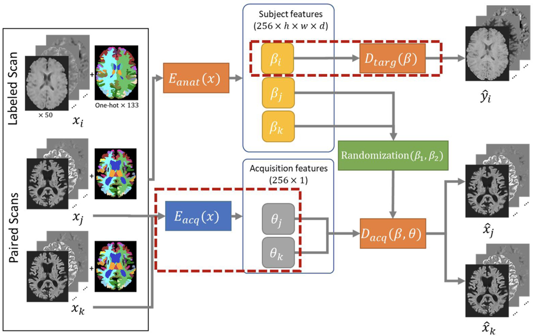
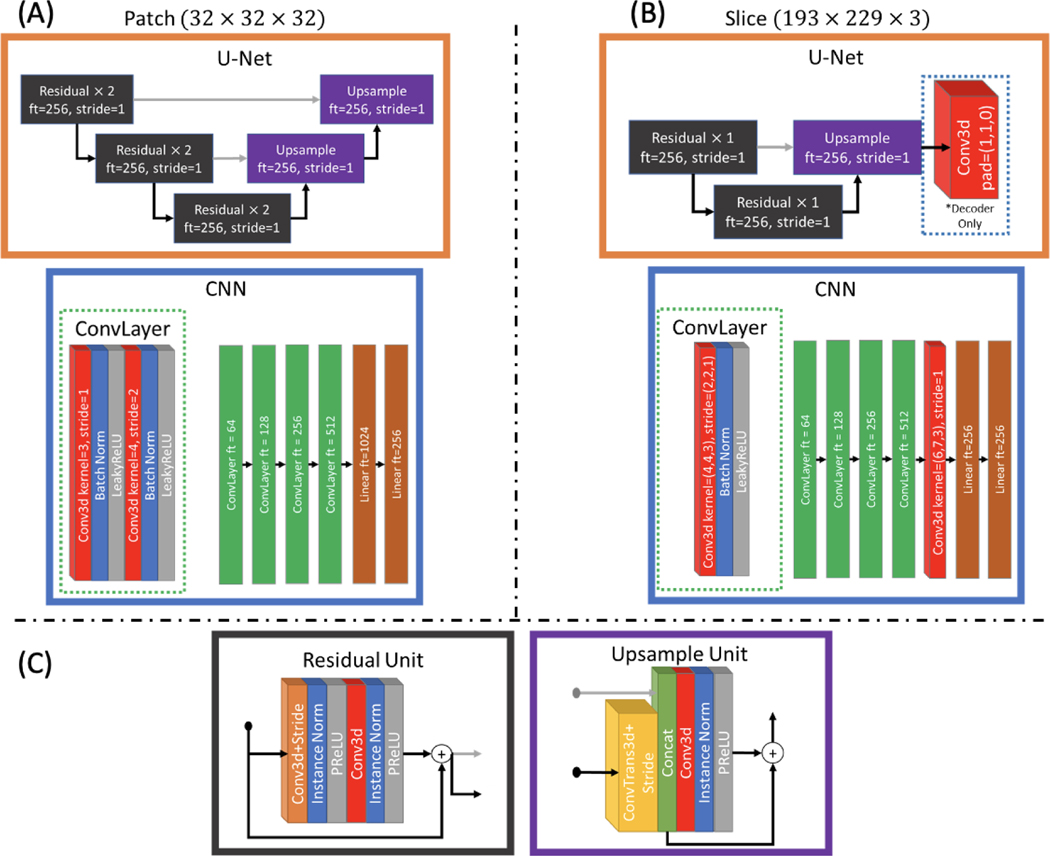
We repurpose the model designed by Dewey et al. to harmonize between sites rather than between contrasts (Figure 3). This method consists of learning two things: the disentanglement between acquisition specific and anatomical specific features and the transformation to the target acquisition. Because cross-site same subject pairs exist within the input data, we can use a pair of scans from different scanners or acquisitions to learn the disentanglement, and we can use the labeled MUSHAC data to learn the transformation from acquisition free latent space. The model is comprised of an anatomical encoder $E_{anat}$, an acquisition encoder $E_{acq}$, an acquisition decoder $D_{acq}$, and a target decoder $D_{targ}$. The architectures of $E_{anat}$, $D_{acq}$, and $D_{targ}$ are modified 3D U-Nets [35, 36] which do not downsample the spatial dimensions of the input. The architecture of $E_{acq}$ is a 3D convolutional neural network which encodes the input in to a 1×256 vector that contains acquisition specific features. The architectures are modified for 32×32×32⁡ patches as well as 193×223×3 slabs of axial slices. The specifics of these architectures are shown in Appendix A.

Figure 3.

We follow the work of Dewey et al., but where before the goal was to harmonize between T1 and T2 acquisitions, our goal is to harmonize between many DW-MRI acquisitions as well move all data to a single target space. Changes to the method are indicated by red boxes. To account for the much broader range of acquisition possibilities, we use an acquisition encoder which represents the acquisition using a vector of size 256 rather than a single value which only needed to indicate contrast. In a similar manner, we use paired subject data from different acquisitions and encourage the network to encode a latent space which represents only the subject specific feature free from scanner or acquisition bias, and then reconstruct the acquisition indicated by the acquisition encoding vector using subject features from either scan. A second decoder was added to learn from the acquisition free latent space to a target space using the supervised data.

For each step in training, a volume from one of the three input sites of the MUSHAC dataset x_i as well as a pair of sites from either the BLSA or MUSHAC [x_j, x_k] are selected. $E_{anat}$, $E_{acq}$, and $D_{acq}$ are trained using the paired data [x_j, x_k] in a similar fashion to Dewey et al. The SHORE coefficients of the input are fed to $E_{anat}$ and $E_{acq}$ for each x_j and x_k resulting in subject features β_j and β_k and acquisition features θ_j and θ_k. For each β feature map, the feature map is randomly taken from β_j or β_k to form β_jk. This encourages the model to represent subject features the same across acquisition. $D_{acq}$ is then given the pairs of [β_jk, θ_j] and [β_jk, θ_k] with the goal of reconstructing the acquisition specified by θ. $D_{targ}$ is given only β_i with the goal of generating the associated target image y_i. $E_{anat}$, $D_{acq}$, and $E_{acq}$ are trained using the paired data [x_j, x_k], while $D_{targ}$ is trained separately using the labeled data [x_i, y_i]. The loss functions employ L1 loss (L1), structural similarity index measure loss (SSIM), total variation loss (TV), and Sobel edge detection (Sobel):

$$L_{image}(x,\widehat{y},y)=SSIM(\widehat{y},y)+L1(\widehat{y},y)+TV(\widehat{y})+L1(Sobel(x),Sobel(\widehat{y}))$$ (3)

where the SSIM and L1 terms encourage the predicted $\widehat{y}$ to have the same information as y, the TV term regularizes neighborhood consistency within $\widehat{y}$, and another L1 term between the edge features of the input x and the prediction $\widehat{y}$ enforces that the structure remains the same. For $E_{anat}$, $D_{acq}$, and $E_{acq}$, the loss function is:

$$L=L_{image}\left(x_j,{\widehat{x}}_j,x_j\right)+L_{image}\left(x_k,{\widehat{x}}_k,x_k\right)+{\lambda }_{E}L1\left({\beta }_j,{\beta }_k\right)$$ (4)

where the final term is a contrastive term which further encourages the structural features to be similar across acquisitions and λ_E controls the contribution of this term and is empirically set to 10. The loss for $D_{targ}$ is:

$$L=L_{image}\left(x_i,{\widehat{y}}_i,y_i\right)$$ (5)

The implementation of this model requires two optimizers, one responsible for each of these losses. We choose each of these to be an Adam optimizer with a learning rate of 1e-5. Each model was trained until convergence on a validation set which was approximately 75 epochs each consisting of approximately 1500 samples of patches or axial slabs. Where the patch-based model was evaluated in 3D, the slice-based model was evaluated only on the middle of the three axial slices.

CycleGAN Model

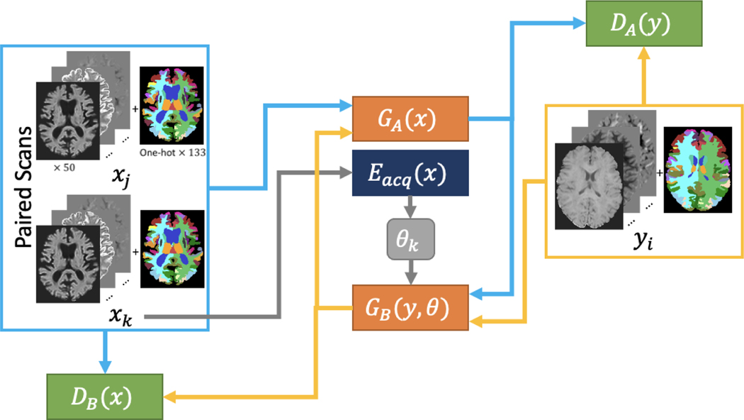
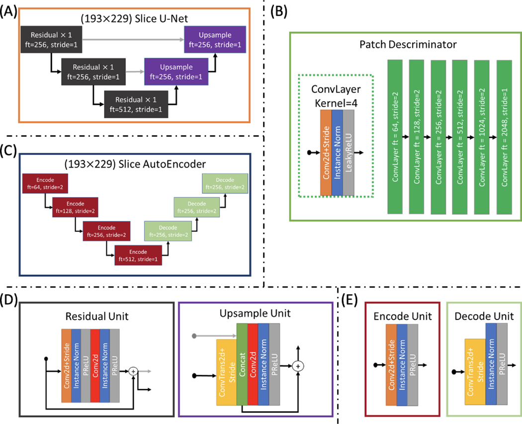
As a baseline representing unsupervised learning approaches, we modify the CycleGAN model according to Bashyam et al. (Figure 4). This involves adding an encoder ($E_{acq}$) which encodes the acquisition specific features of images from the input domain to compensate for potentially many different styles coming from many different acquisitions. Similar to the disentanglement model, the generator which goes from the target domain to the input domain (G_B) is parameterized by a target domain image and the acquisition features which indicate the specific acquisition that should be generated. Also in following Bashyam et al., we pass our input as axial slices rather than slabs or patches. To avoid putting this model at a disadvantage, we also modify the loss to account for paired data which may provide useful information:

$$\begin{gathered} L_G=L2\left(D_A\left(G_A\left(x_j\right)\right),1\right)+{\lambda }_{A}L1\left(G_B\left(G_A\left(x_j\right),E_{acq}\left(x_j\right)\right),x_j\right) \\ +L2\left(D_B\left(G_B\left(y_i,E_{acq}\left(x_j\right)\right)\right),1\right)+{\lambda }_{B}L1\left(G_A\left(G_B\left(y_i,E_{acq}\left(x_j\right)\right)\right),y_i\right) \\ +{\lambda }_{E}L1\left(G_B\left(G_A\left(x_k\right),E_{acq}\left(x_j\right)\right),x_j\right) \end{gathered}$$ (6)

$$\begin{gathered} L_D=L2\left(D_A\left(G_A\left(x_j\right)\right),0\right)+L2\left(D_A\left(y_i\right),1\right)+L2\left(D_B\left(G_B\left(y_i,E_{acq}\left(x_j\right)\right)\right),0\right)+ \\ L2\left(D_B\left(x_j\right),1\right) \end{gathered}$$ (7)

where L_G is the generator loss, L_D is the discriminator loss, G_A is the generator which is parameterized by the input domain and generates the target domain, D_A is the discriminator which classifies between real and fake target domain images, and D_B is the discriminator which classifies between real and fake input domain images. λ_A, λ_B, and λ_E are hyperparameters for the cycle loss terms and are empirically set to 25. The final term of the generator loss is similar to the cycle loss except the goal is to recreate x_j using x_k to parameterize G_A to leverage the paired data. Training consisted of 200 epochs where during the first 100 epoch a learning rate of 2e-5 was used and during the last 100 epochs the learning rate was linearly to zero. The architectures used are shown in Appendix A.

Figure 4.

As a baseline, a CycleGAN framework is constructed from two U-Net generators, one which takes an axial slice of SHORE coefficients and one hot encoded SLANT segmentation from the input domain and generates the target domain and vice versa, as well as two patch discriminators, one which tries to classify whether or not the input is from the input domain and one which does the same for the target domain. Due to the input domain being composed of multiple sites and acquisitions, an autoencoder is used to extract acquisition specific information θ from the input image which is then used as input when trying to generate an input domain image to specify what scanner or acquisition the generated image should resemble.

RESULTS

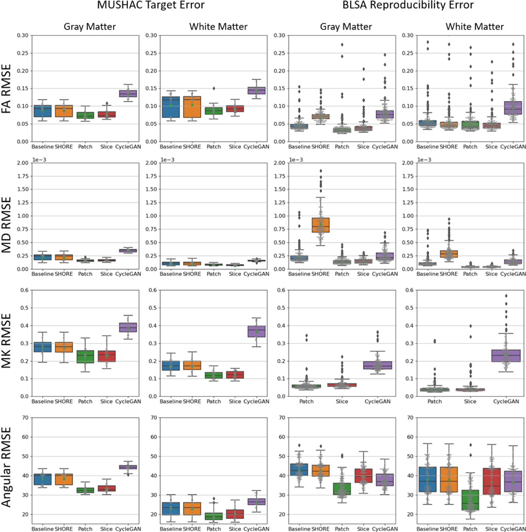
We evaluate each method in terms of RMSE for the metrics fractional anisotropy (FA), mean diffusivity (MD), mean kurtosis (MK), and the angular error of the primary eigenvector (PE) of the diffusion tensor (Figure 5 & Table 4). For the MUSHAC dataset four subjects were withheld for testing and each of the input from the three acquisitions PrismaSA, PrismaST, and ConnectomST are evaluated by their similarity to the target acquisition ConnectomSA. For the BLSA dataset five subjects were withheld for testing and each scan from the 1.5T scanner (A) and the 3T scanners (B, C, or D) are evaluated by their similarity to an average which is calculated for each method. The Wilcoxon signed-rank test was used to test statistical significance of each method (p-value<0.01).

Figure 5.

Here the methods are compared in terms of RMSE of FA, MD, MK, and angular error for each input scan. The baseline and SHORE methods use all available shells while all other methods are given on the first shell of a lower b-value. On average, the Patch and Slice disentanglement models perform better in white and gray matter for both datasets across metrics. Notably the improvement in MK indicates the estimation of the second shell is successful. Wilcoxon signed-rank test shows that all methods are statistically significant (p-value<0.01).

Table 4.

The mean and standard deviation of the RMSE across scans is reported for each dataset in the white matter and gray matter. The lowest RMSE across FA, MD, MK, and Angular error (noted in bold) is achieved by the Patch or Slice disentanglement method.

	Gray Matter				White Matter
Method	FA RMSE	MD RMSE (1e-05)	MK RMSE	Angular RMSE	FA RMSE	MD RMSE (1e-05)	MK RMSE	Angular RMSE
MUSHAC
Baseline	0.088±0.017	22.65±5.48	0.28±0.04	38.55±2.97	0.104±0.029	10.64±3.06	0.17±0.03	23.07±4.33
SHORE	0.088±0.018	22.60±5.57	0.28±0.04	38.53±2.97	0.105±0.030	10.63±3.18	0.17±0.04	23.05±4.34
Patch	0.075±0.011	15.88±2.32	0.23±0.05	32.79±1.68	0.090±0.013	7.86±1.70	0.12±0.02	19.46±2.67
Slice	0.080±0.011	16.39±2.32	0.23±0.04	33.70±1.91	0.096±0.011	7.50±1.29	0.12±0.02	20.61±2.90
CycleGAN	0.218±0.057	48.59±14.15	0.44±0.07	52.36±4.22	0.187±0.030	17.83±3.04	0.35±0.07	41.56±10.90
BLSA
Baseline	0.046±0.017	23.71±13.07	NaN±NaN	41.35±5.56	0.061±0.039	12.16±9.28	NaN±NaN	33.64±9.73
SHORE	0.074±0.014	90.54±25.48	NaN±NaN	41.13±5.46	0.057±0.034	34.66±14.68	NaN±NaN	33.73±9.64
Patch	0.036±0.024	14.24±4.54	0.06±0.02	33.66±4.27	0.050±0.030	3.76±1.51	0.04±0.03	28.17±6.48
Slice	0.041±0.025	13.41±4.17	0.07±0.03	37.95±5.68	0.050±0.026	3.77±1.26	0.05±0.05	32.74±9.77
CycleGAN	0.127±0.045	40.04±17.33	0.18±0.04	37.12±4.10	0.096±0.041	14.48±6.93	0.19±0.07	36.26±7.13

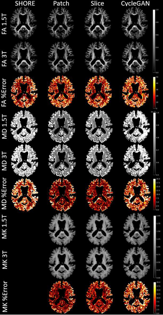
In the MUSHAC data the baseline and SHORE methods are generally similar with some improvement over the baseline in MK and angular error. The disentanglement methods outperform all other methods on average. Additionally, without the second diffusion shell, the model cannot rely on the identity transform to achieve similar results as the baseline. A visualization of the error reveals the differences in the Patch and Slice method (Figure 6). While the Patch method has a small advantage in gray matter regions, the Slice seems to achieve superior performance in the core of the corpus callosum. The CycleGAN method performs poorly at this task, and it can be seen where the model fails to generate the correct anatomy in the sample subject.

Figure 6.

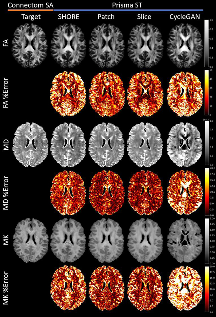
For a single MUSHAC subject an axial slice of FA, MD, and MK and the precent error is shown for each method excluding the baseline. For the disentanglement methods, the error generally improves in both gray and white matter. However, the Slice method shows greater error reduction in white matter.

In the BLSA data, the difference between methods is less distinct, but similar trends appear. Although, the SHORE method has much different behavior due to only being fit with a single-shell. The large increase in reproducibility error in MD in both gray and white matter and in FA in gray matter suggest that the method is not particularly stable for single-shell data. Additionally, there is no baseline or SHORE method for MK due the data only being acquired with a single-shell. Again the disentanglement methods obtain the lowest error for all metrics. However, the angular error for the slice method is greater than the Patch method. Visually it can be seen again that the CycleGAN method is inconsistent.

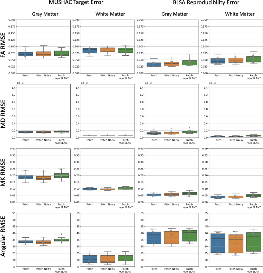
As an ablation, we also train the Patch method on a single fold with data augmented by random Gaussian noise to test the stability of the model (Patch Noisy) and without the anatomical parcellation as a prior (Patch w/o SLANT) to assess the contribution of the T1 derived information. We find that there is a small drop in performance when the SLANT priors are withheld from the model, and we also find the approach is not affected by noisy training data. The results of this ablation experiment are presented in Appendix B.

DISCUSSION

The chosen datasets are each unique and present different challenges for harmonization. The MUSHAC dataset was specifically designed to have two very different acquisition protocols which tends to be the main contribution of reproducibility error compared to the bias introduced by differences in hardware. The BLSA dataset was not intended to have different acquisition parameters, but throughout the course of the study, there were inevitably replacements made resulting in four different hardware and slightly altered acquisition parameters. The aging aspect of the data introduces reproducibility error resulting from actual changes in anatomy rather than scanner or acquisition bias which should be preserved rather than removed or altered. In trying to harmonize all these data to a single target space includes dealing with the differences in b-value, the number of shells, and the anatomical differences in an aging cohort and a young adult cohort.

By choosing a method that represents the diffusion signal as the same set of coefficients regardless of the acquisition, the simplified input space can potentially use a single model. However, the differences between the estimated SHORE coefficients from single-shell data and multi-shell data creates two distinct tasks for the model to learn. This becomes particularly difficult when the unlabeled set of data only contains single-shell representations, and the labeled data only contains multi-shell representations as semi-supervised learning relies on the supervised term to form a good approximation to start learning from the unlabeled data. We choose to only use the first shell for our deep learning methods to avoid this, but it is a considerable limitation. Despite only using a single-shell, the disentanglement models achieve lower MK error overall which is derived from diffusion kurtosis imaging (DKI) and requires multiple shells to be estimated. This suggests that the multi-shell SHORE representation can be approximated well, and that given the choice, harmonizing with a single-shell is better than using multi-shell data as it is.

The choice of the SHORE representation while aiding to overcome multiple acquisition protocols requires that the model accurately represents multiple features in the output space. While some of the 50 coefficients have a larger impact on such measures as MD and FA, for the model to adapt single-shell data to multi-shell, most of the 50 coefficients would need to be accurately estimated, and so we did not influence the models by weighting the loss by coefficient preventing models from placing more importance on a particular coefficient. The CycleGAN model being purely unsupervised did not have the benefit of the highly informative labeled samples and so could not converge on a point where all coefficients were realistic and anatomically correct in our experimental setup. Further investigation to unsupervised approaches is necessary, but outside of the scope of this work.

An interesting aspect of the disentanglement model used here, is that the harmonization between the input takes place entirely in the encoders which are tasked with extracting either the anatomical or the acquisition specific information from the data. By preventing the gradients from the decoder $D_{targ}$ which is tasked with estimating the target site from being backpropagated to the encoder, we ensure that the encoder $E_{anat}$ is fully self-supervised along with the decoder $D_{acq}$. $D_{targ}$ can generate an image when parameterized by the unlabeled BLSA data even though it only learned from the labeled MUSHAC data, because the anatomical latent space which it learns from is free from acquisition specific features.

Though deep learning is a promising approach to harmonization, the advantage of such approaches lies in extracting information from large datasets. As was shown in the challenge associated with the MUSHAC dataset, with only 10 subjects in a supervised training set, regression models can outperform convolutional neural networks with millions of parameters. Additionally, a model trained to transform one site to another is only useful for those who need to harmonize data acquired on those specific scanners or those who have a large enough cohort to retrain the model.

Where deep learning can be the most useful in harmonization is in developing a model which can generalize well to unseen diffusion acquisitions. Because a fully supervised dataset of many subjects covering many acquisition parameters and scanner hardware is time consuming and expensive, it would be beneficial to leverage semi-supervised approaches to bring together many different datasets. Though this work takes a step towards this goal, it is limited to datasets which contain paired data which contain differences in acquisition or hardware between them.

CONCLUSION

The framework provided in this work can reduce error introduced by differences in acquisition and hardware in two unique datasets and can potentially be extended to many datasets provided they contain paired data. We advocate for further development of harmonization models which generalize across many datasets and account for the various differences in acquisition protocols in DW-MRI.

Figure 7.

Here we look at the reproducibility error for each method for a BLSA subject using a scan acquired at the 1.5T scanner (A) and a scan acquired at a 3T scanner (B). Here the difference between the Patch and Slice Disentanglement models is clear in FA where the error in white matter is much lower for the Slice method.

APPENDIX A

Figure 8.

The architectures used in the disentanglement model are modified for 32 by 32 by 32 patches (A) as well as 193 by 229 by 3 axial slabs (B). The acquisition encoder is defined by a CNN which results in a vector of size 256 while the structural encoder and the two decoders are defined by U-Nets which preserve the original size of the input. The U-Nets use the same residual and upsample units (C).

Figure 9.

All architectures for the CycleGAN method are designed for 193 by 229 axial slices. The generators are defined as U-Nets (A), the discriminators are defined as patch discriminators (B), and the acquisition encoder is defined as an autoencoder (C). The residual and upsample units for the U-Net are similar to those used in the disentanglement model (D), and the autoencoder uses similar units which lack the skip connection (E).

APPENDIX B

Figure 10.

We modify the Patch disentanglement model to 1) test the models robustness when trained with data augmented with Gaussian noise and 2) test the models response to removing the anatomical segmentation priors. While the model seems to have a small response to adding noise, removing the anatomical priors generally decreases performance. Wilcoxon signed-rank test shows that all methods are statistically significant (p-value<0.01).

REFERENCES

- 1.Le Bihan D, Looking into the functional architecture of the brain with diffusion MRI. Nature Reviews Neuroscience, 2003. 4(6): p. 469–480. [DOI] [PubMed] [Google Scholar]
- 2.Le Bihan D and Johansen-Berg H, Diffusion MRI at 25: exploring brain tissue structure and function. Neuroimage, 2012. 61(2): p. 324–341. [DOI] [PMC free article] [PubMed] [Google Scholar]
- 3.Vollmar C, et al. , Identical, but not the same: intra-site and inter-site reproducibility of fractional anisotropy measures on two 3.0 T scanners. Neuroimage, 2010. 51(4): p. 1384–1394. [DOI] [PMC free article] [PubMed] [Google Scholar]
- 4.Matsui JT, Development of image processing tools and procedures for analyzing multisite longitudinal diffusion-weighted imaging studies. 2014.
- 5.Zhu T, et al. , Quantification of accuracy and precision of multi-center DTI measurements: a diffusion phantom and human brain study. Neuroimage, 2011. 56(3): p. 1398–1411. [DOI] [PMC free article] [PubMed] [Google Scholar]
- 6.Jovicich J, et al. , Multisite longitudinal reliability of tract-based spatial statistics in diffusion tensor imaging of healthy elderly subjects. Neuroimage, 2014. 101: p. 390–403. [DOI] [PubMed] [Google Scholar]
- 7.Teipel SJ, et al. , Multicenter stability of diffusion tensor imaging measures: a European clinical and physical phantom study. Psychiatry Research: Neuroimaging, 2011. 194(3): p. 363–371. [DOI] [PubMed] [Google Scholar]
- 8.Rogers BP, et al. Stability of gradient field corrections for quantitative diffusion MRI. in Medical Imaging 2017: Physics of Medical Imaging. 2017. International Society for Optics and Photonics. [DOI] [PMC free article] [PubMed] [Google Scholar]
- 9.Bammer R, et al. , Analysis and generalized correction of the effect of spatial gradient field distortions in diffusion‐weighted imaging. Magnetic Resonance in Medicine: An Official Journal of the International Society for Magnetic Resonance in Medicine, 2003. 50(3): p. 560–569. [DOI] [PubMed] [Google Scholar]
- 10.Tao AT, et al. , Improving apparent diffusion coefficient accuracy on a compact 3T MRI scanner using gradient nonlinearity correction. Journal of Magnetic Resonance Imaging, 2018. 48(6): p. 1498–1507. [DOI] [PMC free article] [PubMed] [Google Scholar]
- 11.Newitt DC, et al. , Gradient nonlinearity correction to improve apparent diffusion coefficient accuracy and standardization in the american college of radiology imaging network 6698 breast cancer trial. Journal of Magnetic Resonance Imaging, 2015. 42(4): p. 908–919. [DOI] [PMC free article] [PubMed] [Google Scholar]
- 12.Malyarenko DI, Ross BD, and Chenevert TL, Analysis and correction of gradient nonlinearity bias in apparent diffusion coefficient measurements. Magnetic resonance in medicine, 2014. 71(3): p. 1312–1323. [DOI] [PMC free article] [PubMed] [Google Scholar]
- 13.Fortin J-P, et al. , Harmonization of multi-site diffusion tensor imaging data. Neuroimage, 2017. 161: p. 149–170. [DOI] [PMC free article] [PubMed] [Google Scholar]
- 14.Mirzaalian H, et al. , Inter-site and inter-scanner diffusion MRI data harmonization. NeuroImage, 2016. 135: p. 311–323. [DOI] [PMC free article] [PubMed] [Google Scholar]
- 15.Koppers S, et al. Spherical harmonic residual network for diffusion signal harmonization. in International Conference on Medical Image Computing and Computer-Assisted Intervention. 2018. Springer. [Google Scholar]
- 16.Moyer D, et al. , Scanner Invariant Representations for Diffusion MRI Harmonization. arXiv preprint arXiv:1904.05375, 2019. [DOI] [PMC free article] [PubMed]
- 17.Koppers S, Haarburger C, and Merhof D. Diffusion MRI signal augmentation: from single shell to multi shell with deep learning. in International Conference on Medical Image Computing and Computer-Assisted Intervention. 2016. Springer. [Google Scholar]
- 18.Nath V, et al. Inter-scanner harmonization of high angular resolution DW-MRI using null space deep learning. in International Conference on Medical Image Computing and Computer-Assisted Intervention. 2018. Springer. [PMC free article] [PubMed] [Google Scholar]
- 19.Dewey BE, et al. A Disentangled Latent Space for Cross-Site MRI Harmonization. in International Conference on Medical Image Computing and Computer-Assisted Intervention. 2020. Springer. [Google Scholar]
- 20.Johnson WE, Li C, and Rabinovic A, Adjusting batch effects in microarray expression data using empirical Bayes methods. Biostatistics, 2007. 8(1): p. 118–127. [DOI] [PubMed] [Google Scholar]
- 21.Chen T, et al. A simple framework for contrastive learning of visual representations. in International conference on machine learning. 2020. PMLR. [Google Scholar]
- 22.He K, et al. Momentum contrast for unsupervised visual representation learning. in Proceedings of the IEEE/CVF conference on computer vision and pattern recognition. 2020. [Google Scholar]
- 23.Modanwal G, et al. MRI image harmonization using cycle-consistent generative adversarial network. in Medical Imaging 2020: Computer-Aided Diagnosis. 2020. International Society for Optics and Photonics. [Google Scholar]
- 24.Palladino JA, Slezak DF, and Ferrante E. Unsupervised domain adaptation via CycleGAN for white matter hyperintensity segmentation in multicenter MR images. in 16th International Symposium on Medical Information Processing and Analysis. 2020. International Society for Optics and Photonics. [Google Scholar]
- 25.Bashyam VM, et al. , Medical Image Harmonization Using Deep Learning Based Canonical Mapping: Toward Robust and Generalizable Learning in Imaging. arXiv preprint arXiv:2010.05355, 2020.
- 26.Ozarslan E, et al. , Simple harmonic oscillator based reconstruction and estimation for three-dimensional q-space MRI. 2009.
- 27.Merlet SL and Deriche R, Continuous diffusion signal, EAP and ODF estimation via compressive sensing in diffusion MRI. Medical image analysis, 2013. 17(5): p. 556–572. [DOI] [PubMed] [Google Scholar]
- 28.Nath V, et al. Enabling multi-shell b-value generalizability of data-driven diffusion models with deep SHORE. in International Conference on Medical Image Computing and Computer-Assisted Intervention. 2019. Springer. [DOI] [PMC free article] [PubMed] [Google Scholar]
- 29.Tax CM, et al. , Cross-scanner and cross-protocol diffusion MRI data harmonisation: A benchmark database and evaluation of algorithms. NeuroImage, 2019. 195: p. 285–299. [DOI] [PMC free article] [PubMed] [Google Scholar]
- 30.Andersson JL, Skare S, and Ashburner J, How to correct susceptibility distortions in spin-echo echo-planar images: application to diffusion tensor imaging. Neuroimage, 2003. 20(2): p. 870–888. [DOI] [PubMed] [Google Scholar]
- 31.Jenkinson M, et al. , FSL. Neuroimage, 2012. 62: p. 782–90. [DOI] [PubMed] [Google Scholar]
- 32.Klein A, et al. Open labels: online feedback for a public resource of manually labeled brain images. in 16th Annual Meeting for the Organization of Human Brain Mapping. 2010. [Google Scholar]
- 33.Huo Y, et al. , 3D whole brain segmentation using spatially localized atlas network tiles. NeuroImage, 2019. 194: p. 105–119. [DOI] [PMC free article] [PubMed] [Google Scholar]
- 34.Garyfallidis E, et al. , Dipy, a library for the analysis of diffusion MRI data. Frontiers in neuroinformatics, 2014. 8: p. 8. [DOI] [PMC free article] [PubMed] [Google Scholar]
- 35.Çiçek Ö, et al. 3D U-Net: learning dense volumetric segmentation from sparse annotation. in International conference on medical image computing and computer-assisted intervention. 2016. Springer. [Google Scholar]
- 36.Ronneberger O, Fischer P, and Brox T. U-net: Convolutional networks for biomedical image segmentation. in International Conference on Medical image computing and computer-assisted intervention. 2015. Springer. [Google Scholar]