Naked Singularities in the Einstein-Euler System

Abstract

In 1990, based on numerical and formal asymptotic analysis, Ori and Piran predicted the existence of selfsimilar spacetimes, called relativistic Larson-Penston solutions, that can be suitably flattened to obtain examples of spacetimes that dynamically form naked singularities from smooth initial data, and solve the radially symmetric Einstein-Euler system. Despite its importance, a rigorous proof of the existence of such spacetimes has remained elusive, in part due to the complications associated with the analysis across the so-called sonic hypersurface. We provide a rigorous mathematical proof. Our strategy is based on a delicate study of nonlinear invariances associated with the underlying non-autonomous dynamical system to which the problem reduces after a selfsimilar reduction. Key technical ingredients are a monotonicity lemma tailored to the problem, an ad hoc shooting method developed to construct a solution connecting the sonic hypersurface to the so-called Friedmann solution, and a nonlinear argument to construct the maximal analytic extension of the solution. Finally, we reformulate the problem in double-null gauge to flatten the selfsimilar profile and thus obtain an asymptotically flat spacetime with an isolated naked singularity.

Introduction

We study the Einstein-Euler system which couples the Einstein field equations to the Euler equations of fluid mechanics. The unknowns are the 4-dimensional Lorentzian spacetime $(\mathcal{M},g)$, the fluid pressure p, the mass-density $\rho$, and the 4-velocity $u^{\alpha }$. In an arbitrary coordinate system, the Einstein-Euler equations read

$$\begin{array}{cc}\hfill {\text{Ric}}_{\alpha \beta }-\frac{1}{2}\mathcal{R}{g}_{\alpha \beta }& =T_{\alpha \beta },(\alpha ,\beta =0,1,2,3),\hfill \end{array}$$ 1.1

$$\begin{array}{cc}\hfill {\mathrm{\nabla }}_{\alpha }{T}^{\alpha \beta }& =0,(\beta =0,1,2,3),\hfill \end{array}$$ 1.2

$$\begin{array}{cc}\hfill g_{\alpha \beta }{u}^{\alpha }{u}^{\beta }& =-1,\hfill \end{array}$$ 1.3

where ${\text{Ric}}_{\alpha \beta }$ is the Ricci curvature tensor, $\mathcal{R}$ the scalar curvature of $g_{\alpha \beta }$, and $T_{\alpha \beta }$ is the energy momentum tensor given by the formula

$$\begin{array}{c}\hfill T_{\alpha \beta }=(\rho +p)u_{\alpha }{u}_{\beta }+p{g}_{\alpha \beta },(\alpha ,\beta =0,1,2,3).\end{array}$$ 1.4

To close the system, we assume the linear equation of state

$$\begin{array}{c}\hfill p=\epsilon \rho ,\end{array}$$ 1.5

where $0<\epsilon <1$ corresponds to the square of the speed of sound.

The system (1.1)–(1.5) is a fundamental model of a selfgravitating relativistic gas. We are interested in the existence of selfsimilar solutions to (1.1)–(1.5) under the assumption of radial symmetry. This amounts to the existence of a homothetic Killing vector field $\xi$ with the property

$$\begin{array}{c}\hfill {\mathcal{L}}_{\xi }g=2g,\end{array}$$ 1.6

where the left-hand side is the Lie derivative of the metric g. The presence of such a vector field induces a scaling symmetry, which allows us to look for selfsimilar solutions to (1.1)–(1.5). Study of selfsimilar solutions to Einstein-matter systems has a rich history in the physics literature. They in particular provide a way of constructing spacetimes with so-called naked singularities, a notion intimately tied to the validity of the weak cosmic censorship of Penrose [30], see the discussion in [7, 10, 32]. Naked singularities intuitively correspond to spacetime singularities that are “visible" to far away observers, which informally means that there exists a future outgoing null-geodesic “emanating" from the singularity and reaching the asymptotically flat region of the spacetime. We adopt here a precise mathematical definition from the work of Rodnianski and Shlapentokh-Rothman [32, Definition 1.1], which in turn is related to a formulation of weak cosmic censorship by Christodoulou [7].

In the absence of pressure ($\epsilon =0$ in (1.5)) and under the assumption of radial symmetry, the problem simplifies considerably. The corresponding family of solutions was studied by Lemaître [21] and Tolman [34] in early 1930s (see also [1]). In their seminal work from 1939, Oppenheimer and Snyder [25] studied the causal structure of a subclass of Lemaître-Tolman solutions with space-homogeneous densities, thus exhibiting the first example of a dynamically forming (what later became known as) black hole. However, in 1984 Christodoulou [5] showed that, within the larger class of Lemaître-Tolman solutions with space-inhomogeneous densities, black holes are exceptional and instead naked singularities form generically.

Of course, in the context of astrophysics, one expects the role of pressure to be very important in the process of gravitational collapse for relativistic gases. In the late stages of collapse, the core region is expected to be very dense and the linear equation of state (1.5) is commonly used in such a setting, as it is compatible with the requirement that the speed of sound is smaller than the speed of light, $\sqrt{\epsilon }<1$. In their pioneering works, Ori and Piran [26–28] found numerically selfsimilar solutions to (1.1)–(1.5), which are the relativistic analogues of the Larson-Penston selfsimilar collapsing solutions to the isothermal Euler-Poisson system, see [15, 20, 31]. Through both numerical and asymptotic analysis methods Ori and Piran investigated the causal structure of such relativistic Larson-Penston solutions, ascertaining the existence of spacetimes with naked singularities when $\epsilon$ is smaller than a certain value. Our main goal is to justify the findings of Ori and Piran on rigorous mathematical grounds.

Broadly speaking, this manuscript consists of two parts. In the first part, which constitutes the bulk of our work, we construct a selfsimilar solution of the Einstein-Euler system (Sections 3–8), assuming that $\epsilon$ – the square of the speed of sound – is sufficiently small.

Theorem 1.1

(Existence of the relativistic Larson-Penston spacetimes) For any sufficiently small $0<\epsilon \ll 1$ there exists a radially symmetric real-analytic selfsimilar solution to the Einstein-Euler system with a curvature singularity at the scaling origin and an outgoing null-geodesic emanating from it all the way to infinity. The resulting spacetime is called the relativistic Larson-Penston (RLP) spacetime.

It is not hard to see that the selfsimilar solution constructed in Theorem 1.1 is not asymptotically flat. In the second step (Section 9), using PDE techniques, we flatten the selfsimilar RLP-profile in a region away from the singularity and thus obtain an asymptotically flat solution with a naked singularity. Thus, our main theorem states that in the presence of pressure there do exist examples of naked singularities which form from smooth data.

Theorem 1.2

(Existence of naked singularities) For sufficiently small $0<\epsilon \ll 1$ there exist radially symmetric asymptotically flat solutions to the Einstein-Euler system that form a naked singularity in the sense of [32, Definition 1.1].

Other than the dust-Einstein model mentioned above, we are aware of two other rigorous results on the existence of naked singularities. In 1994 Christodoulou [6] provided a rigorous proof of the existence of radially symmetric solutions to the Einstein-scalar field system, which contain naked singularities (see also [8] for the proof of their instability). Very recently, Rodnianski and Shlapentokh-Rothman [32] proved the existence of solutions to the Einstein-vacuum equations which contain naked singularities and are (necessarily) not radially symmetric.

In the physics literature much attention has been given to selfsimilar solutions and naked singularities for the Einstein-Euler system, see for example [2, 14]. A selfsimilar reduction of the problem was first given in [33]. As explained above, a detailed analysis of the resulting equations, including the discussion of naked singularities, was given in [26–28]. Subsequent to [28], a further analysis of the causal structure, including the nonradial null-geodesics was presented in [19], see also [4]. There exist various approaches to the existence of solutions to the selfsimilar problem, most of them rely on numerics [3, 17, 28]. A dynamical systems approach with a discussion of some qualitative properties of the solutions was developed in [3, 13]. Numerical investigation of the stability of the RLP-spacetimes can be found in [17, 18]. selfsimilar relativistic perfect fluids play an important role in the study of the so-called critical phenomena - we refer to reviews [14, 24].

The proof of Theorem 1.1 relies on a careful study of the nonlinear invariances of the finite-dimensional non-autonomous dynamical system obtained through the selfsimilar reduction. The solutions we construct are real-analytic in a suitable choice of coordinates. A special role is played by the so-called sonic line (sonic point), the boundary of the backward sound cone emanating from the scaling origin $\mathcal{O}$. Many difficulties in the proof of Theorem 1.1 originate from possible singularities across this line, which together with the requirement of smoothness, puts severe limitations on the possible space of smooth selfsimilar solutions. We are aware of no general ODE theory for global existence in the presence of singular sonic points. Therefore, our proofs are all based on continuity arguments, where we extract many delicate invariant properties of the nonlinear flow, specific to the ODE system at hand. In particular, the discovery of a crucial monotonicity lemma enables us to apply an ad hoc shooting method, which was developed for the limiting Larson-Penston solution in the non-relativistic context by the authors. From the point of view of fluid mechanics, the singularity at $\mathcal{O}$ is an imploding one, as the energy density blows up on approach to $\mathcal{O}$. It is in particular not a shock singularity.

The asymptotic flattening in Theorem 1.2 requires solving a suitable characteristic problem for the Einstein-Euler system formulated in the double-null gauge. We do this in a semi-infinite characteristic rectangular domain wherefrom the resulting solution can be glued smoothly to the exact selfsimilar solution in the region around the singularity $\mathcal{O}$. The proof of Theorem 1.2 is given in Section 9.6.

Due to the complexity of our analysis, in Section 2 we give an extensive overview of our methods and key ideas behind the detailed proofs in Sections 3–9.

Methodology and Outline

Formulation of the Problem (Section 3)

Following [28] it is convenient to work with the comoving coordinates

$$\begin{array}{c}\hfill g=-e^{2\mu (\tau ,R)}d{\tau }^2+e^{2\lambda (\tau ,R)}d{R}^2+r^2(\tau ,R)\gamma ,\end{array}$$ 2.7

where $\gamma ={\gamma }_{\mathit{AB}}d{x}^{A}d{x}^B$ is the standard metric on ${\mathbb{S}}^2$, $x^A$, $A=2,3$ are local coordinates on ${\mathbb{S}}^2$, and r is the areal radius. The vector field ${\partial }_{\tau }$ is chosen in such a way that the four velocity $u^{\nu }$ is parallel to ${\partial }_{\tau }$. The normalisation condition (1.3) then implies

$$\begin{array}{c}\hfill u=e^{-\mu }{\partial }_{\tau }.\end{array}$$ 2.8

The coordinate R acts as a particle label. The coordinates $(\tau ,R)$ are then uniquely determined by fixing the remaining gauge freedoms in the problem, the value of $\mu (\tau ,R){|}_{R=0}$ and by setting $r(-1,R)=R$, which states that on the hypersurface $\tau =-1$ the comoving label R coincides with the areal radius.

Introduce the radial velocity

$$\begin{array}{c}\hfill \mathcal{V}:=e^{-\mu }{\partial }_{\tau }r,\end{array}$$ 2.9

the Hawking (also known as Misner-Sharp) mass

$$\begin{array}{c}\hfill m(\tau ,R):=4\pi {\int }_0^{r(\tau ,R)}\rho s^{2}ds=4\pi {\int }_0^R\rho r^2{\partial }_{R}rd\overline{R},\end{array}$$ 2.10

and the mean density

$$\begin{array}{c}\hfill G(\tau ,R):=\frac{m(\tau ,R)}{\frac{4\pi }{3}r{(\tau ,R)}^3}=\frac{3}{r{(\tau ,R)}^3}{\int }_0^R\rho (\tau ,\overline{R})r{(\tau ,\overline{R})}^2{\partial }_{R}r(\tau ,\overline{R})d\overline{R}.\end{array}$$ 2.11

Recalling the equation of state (1.5), the spherically symmetric Einstein-Euler system in comoving coordinates reads (see [12, 23])

$$\begin{array}{cc}\hfill {\partial }_{\tau }\rho +(1+\epsilon )\rho \left(\frac{{\partial }_R\mathcal{V}}{{\partial }_{R}r},+,2,\frac{\mathcal{V}}{r}\right)e^{\mu }& =0,\hfill \end{array}$$ 2.12

$$\begin{array}{cc}\hfill {\partial }_{\tau }\lambda & =e^{\mu }\frac{{\partial }_R\mathcal{V}}{{\partial }_{R}r},\hfill \end{array}$$ 2.13

$$\begin{array}{cc}\hfill e^{-\mu }{\partial }_{\tau }\mathcal{V}+\frac{\epsilon }{1+\epsilon }\frac{{\partial }_{R}r{e}^{-2\lambda }}{\rho }{\partial }_R\rho +4\pi r\left(\frac{1}{3},G,+,\epsilon ,\rho \right)& =0,\hfill \end{array}$$ 2.14

$$\begin{array}{cc}\hfill {({\partial }_{R}r)}^2{e}^{-2\lambda }& =1+{\mathcal{V}}^2-\frac{8\pi }{3}G{r}^2,\hfill \end{array}$$ 2.15

where we recall (2.11). The well-known Tolman-Oppenheimer-Volkov relation reads $(\rho +p){\partial }_R\mu +{\partial }_{R}p=0$, which after plugging in (1.5) further gives the relation

$$\begin{array}{c}\hfill {\partial }_R\mu =-\frac{\epsilon }{1+\epsilon }\frac{{\partial }_R\rho }{\rho }.\end{array}$$ 2.16

Comoving Selfsimilar Formulation

It is straightforward to check that the system (2.12)–(2.15) is invariant under the scaling transformation

$$\begin{array}{c}\hfill \rho \mapsto a^{-2}\rho (s,y),r\mapsto ar(s,y),\mathcal{V}\mapsto \mathcal{V}(s,y),\lambda \mapsto \lambda (s,y),\mu \mapsto \mu (s,y),\end{array}$$ 2.17

where the comoving “time" $\tau$ and the particle label R scale according to

$$\begin{array}{c}\hfill s=\frac{\tau }{a},y=\frac{R}{a},a>0.\end{array}$$ 2.18

Motivated by the scaling invariance (2.17)–(2.18), we look for selfsimilar spacetimes of the form

$$\begin{array}{cc}\hfill \rho (\tau ,R)& =\frac{1}{2\pi {\tau }^2}\mathrm{\Sigma }(y),\hfill \end{array}$$ 2.19

$$\begin{array}{cc}\hfill r(\tau ,R)& =-\sqrt{\epsilon }\tau \tilde{r}(y),\hfill \end{array}$$ 2.20

$$\begin{array}{cc}\hfill \mathcal{V}(\tau ,R)& =\sqrt{\epsilon }V(y),\hfill \end{array}$$ 2.21

$$\begin{array}{cc}\hfill \lambda (\tau ,R)& =\lambda (y),\hfill \end{array}$$ 2.22

$$\begin{array}{cc}\hfill \mu (\tau ,R)& =\mu (y),\hfill \end{array}$$ 2.23

$$\begin{array}{cc}\hfill G(\tau ,R)& =\frac{1}{4\pi {\tau }^2}\tilde{G}(y)=\frac{3}{2\pi {\tau }^2{\tilde{r}}^3}{\int }_0^y\mathrm{\Sigma }(\tilde{y}){\tilde{r}}^2{\tilde{r}}^{\prime }d\tilde{y},\hfill \end{array}$$ 2.24

where

$$\begin{array}{c}\hfill y=\frac{R}{-\sqrt{\epsilon }\tau }.\end{array}$$ 2.25

Associated with the comoving selfsimilar coordinates are the two fundamental unknowns:

$$\begin{array}{cc}\hfill \mathbf{d}& :={\mathrm{\Sigma }}^{\frac{1-\epsilon }{1+\epsilon }},\hfill \end{array}$$ 2.26

$$\begin{array}{cc}\hfill \mathbf{w}& :=(1+\epsilon )\frac{e^{\mu }V+\tilde{r}}{\tilde{r}}-\epsilon .\hfill \end{array}$$ 2.27

For future use it is convenient to sometimes consider the quantity

$$\begin{array}{c}\hfill \mathit{\chi }(y):=\frac{\tilde{r}(y)}{y},\end{array}$$ 2.28

instead of $\tilde{r}$. Quantity $\mathbf{d}$ corresponds to the selfsimilar number density, while $\mathbf{w}$ is referred to as the relative velocity. It is shown in Proposition 3.4 that the radial Einstein-Euler system under the selfsimilar ansatz above reduces to the following system of ODE:

$$\begin{array}{cc}\hfill {\mathbf{d}}^{\prime }& =-\frac{2(1-\epsilon )\mathbf{d}(\mathbf{d}-\mathbf{w})}{(1+\epsilon )y(e^{2\mu -2\lambda }{y}^{-2}-1)},\hfill \end{array}$$ 2.29

$$\begin{array}{cc}\hfill {\mathbf{w}}^{\prime }& =\frac{(\mathbf{w}+\epsilon )(1-3\mathbf{w})}{(1+\epsilon )y}+\frac{2\mathbf{w}(\mathbf{d}-\mathbf{w})}{y(e^{2\mu -2\lambda }{y}^{-2}-1)}.\hfill \end{array}$$ 2.30

This formulation of the selfsimilar problem highlights the danger from possible singularities associated with the vanishing of the denominators on the right-hand side of (2.29)–(2.30). Such points play a distinguished role in our analysis, and as we shall show shortly, are unavoidable in the study of physically interesting selfsimilar solutions.

Definition 2.1

(The sonic point) For any smooth solution to (2.29)–(2.30) we refer to a point $y_{\ast }\in (0,\infty )$ satisfying

$$\begin{array}{c}\hfill y_{\ast }^2=e^{2\mu (y_{\ast })-2\lambda (y_{\ast })}\end{array}$$ 2.31

as the sonic point.

Schwarzschild Selfsimilar Formulation

The comoving formulation (2.29)–(2.30) as written does not form a closed system of ODE. To do so, we must express the metric coefficients $\mu ,\lambda$ as functions of $\mathbf{d},\mathbf{w}$, which can be done at the expense of working with $\tilde{r}$ (or equivalently $\mathit{\chi }$) as a further unknown. To avoid this, it is possible to introduce the so-called Schwarzschild selfsimilar coordinate:

$$\begin{array}{c}\hfill x:=\tilde{r}(y)\end{array}$$ 2.32

so that

$$\begin{array}{c}\hfill \frac{\mathit{dx}}{\mathit{dy}}={\tilde{r}}^{\prime }=\frac{x(\mathbf{w}+\epsilon )}{y(1+\epsilon )}.\end{array}$$ 2.33

In this coordinate system the problem takes on a form analogous to the Eulerian formulation of the selfsimilar Euler-Poisson system from [15]. It is shown in Lemma 3.5 that the new unknowns

$$\begin{array}{c}\hfill D(x):=\mathbf{d}(y),W(x):=\mathbf{w}(y),\end{array}$$ 2.34

solve the system

$$\begin{array}{cc}\hfill D^{\prime }(x)& =-\frac{2x(1-\epsilon )D(W+\epsilon )(D-W)}{B},\hfill \end{array}$$ 2.35

$$\begin{array}{cc}\hfill W^{\prime }(x)& =\frac{(1-3W)}{x}+\frac{2x(1+\epsilon )W(W+\epsilon )(D-W)}{B},\hfill \end{array}$$ 2.36

where

$$\begin{array}{c}\hfill B=B[x;D,W]:=D^{-\eta }-\left[{(W+\epsilon )}^2,-,\epsilon ,{(W-1)}^2,+,4,\epsilon ,D,W\right]x^2,\end{array}$$ 2.37

and

$$\begin{array}{c}\hfill \eta :=\frac{2\epsilon }{1-\epsilon }.\end{array}$$ 2.38

The Greek letter $\eta$ will always be used to mean (2.38) in the rest of the paper. In this formulation, sonic points correspond to zeroes of $B=B[x;D,W]$, i.e. if $y_{\ast }$ is a sonic point in the sense of Definition 2.1, then $x_{\ast }:=\tilde{r}(y_{\ast })$ is a zero of the denominator B.

Friedmann, Far-Field, and the Necessity of the Sonic Point

There are two exact solutions to (2.35)–(2.36). The far-field solution

$$\begin{array}{c}\hfill D_f(x)={(1-\epsilon )}^{-\frac{2}{1+\eta }}{x}^{-\frac{2}{1+\eta }},W_f(x)=1,\end{array}$$ 2.39

features a density $D$ that blows up at $x=0$ and decays to 0 as $x\to \infty$. On the other hand, the Friedmann solution

$$\begin{array}{c}\hfill D_F(x)=\frac{1}{3},W_F(x)=\frac{1}{3},\end{array}$$ 2.40

is bounded at $x=0$, but the density does not decay as $x\to \infty$. Our goal is to construct a smooth solution to (2.35)-(2.36) which qualitatively behaves like the far-field solution as $x\to \infty$ and like the Friedmann solution as $x\to 0^{+}$. We can therefore think of it as a heteroclinic orbit for the dynamical system (2.35)-(2.36). It is then easy to see that any such solution has the property ${lim}_{x\to \infty }B=-\infty$ and ${lim}_{x\to 0^{+}}B(x)>0$. By the intermediate value theorem there must exist a point where B vanishes, i.e. a sonic point.

It is important to understand the formal Newtonian limit, which is obtained by letting $\epsilon =0$ in (2.35)–(2.36). This yields the system

$$\begin{array}{cc}\hfill {\tilde{D}}^{\prime }(x)& =-\frac{2x\tilde{D}\tilde{W}(\tilde{D}-\tilde{W})}{1-x^2{\tilde{W}}^2},\hfill \end{array}$$ 2.41

$$\begin{array}{cc}\hfill {\tilde{W}}^{\prime }(x)& =\frac{(1-3\tilde{W})}{x}+\frac{2x{\tilde{W}}^2(\tilde{D}-\tilde{W})}{1-x^2{\tilde{W}}^2},\hfill \end{array}$$ 2.42

which is precisely the selfsimilar formulation of the isothermal Euler-Poisson system. In [15] we showed that there exists a solution to (2.41)–(2.42) satisfying $\tilde{W}(0)=\frac{1}{3}$, ${lim}_{x\to \infty }\tilde{W}(x)=1$, $\tilde{D}(0)>\frac{1}{3}$, and $\tilde{D}{\asymp }_{x\to \infty }{x}^{-2}$.1 The behaviour of the relativistic solutions when $0<\epsilon \ll 1$ in the region $x\in [0,\infty )$ is modelled on this solution, called the Larson-Penston (LP) solution.

The system (2.35)–(2.37) is a non-autonomous $2\times 2$ system of ODE which is at the heart of the proof of Theorem 1.1 and is used to show the existence of the RLP-solution in the region $x\in [0,\infty )$. As $x\to \infty$, we are forced to switch back to a version of the comoving variables in order to extend the solution beyond $x=\infty$ in a unique way, see the discussion in Section 2.5. A version of the comoving formulation (2.29)–(2.30) plays a crucial role in that extension. In our analysis of the radial null-geodesics (Section 8) and the nonradial ones (Appendix B), we often switch between different choices of coordinates to facilitate our calculations.

Even though the smallness of $\epsilon$ is crucial for the validity of our estimates, we emphasise that we do not use perturbation theory to construct the relativistic solution, by for example perturbing away from the Newtonian one. Such an argument is a priori challenging due to the singular nature of the sonic point, as well as complications arising from boundary conditions.

We mention that selfsimilar imploding flows for the compressible Euler system, featuring a sonic point, were constructed recently in the pioneering work of Merle, Raphaël, Rodnianski, and Szeftel [22] - here the associated $2\times 2$ dynamical system is autonomous. In the context of the Euler-Poisson system with polytropic gas law, selfsimilar collapsing solutions featuring a sonic point were recently constructed in [16].

The Sonic Point Analysis (Section 4)

The solution we are trying to construct is on one hand assumed to be smooth, but it also must feature an a priori unknown sonic point, which we name $x_{\ast }$. This is a singular point for the dynamical system and the assumption of smoothness therefore imposes a hierarchy of constraints on the Taylor coefficients of a solution in a neighbourhood of $x_{\ast }$. More precisely, we look for solutions $(D,W)$ to (2.35)-(2.36) of the form

$$\begin{array}{c}\hfill D=\sum _{N=0}^{\infty }{D}_N{(x-x_{\ast })}^N,W=\sum _{N=0}^{\infty }{W}_N{(x-x_{\ast })}^N.\end{array}$$ 2.43

It is clear that the first constraint reads $D_0=W_0$, as the numerator in (2.35) must vanish at $x_{\ast }$ for the solution to be smooth. Together with the condition $B(x_{\ast })=0$, we can show that for any $\epsilon >0$ sufficiently small, $D_0=W_0$ is a function of $x_{\ast }$, which converges to $\frac{1}{x_{\ast }}$ as $\epsilon \to 0$ in accordance with the limiting Newtonian problem (2.41)–(2.42). Our goal is to express $D_N,W_N$ recursively in terms of $D_0,\cdots ,D_{N-1}$, $W_0,\cdots ,W_{N-1}$ and thus obtain a hierarchy of algebraic relations that allows to compute the Taylor coefficients up to an arbitrary order.

However, an intriguing dichotomy emerges. At the next order, one obtains a cubic equation for $W_1$, see Lemma 4.7. One of the solutions is a “ghost" solution and therefore unphysical, while the remaining two roots, when real, are both viable candidates for $W_1$, given as a function of $D_0$ (and therefore $x_{\ast }$). This is related to an analogous dichotomy in the Newtonian case - where one choice of the root leads to so-called Larson-Penston-type (LP type) solutions, while the other choice of the root leads to Hunter-type solutions. Based on this, for any $0<\epsilon \ll 1$ sufficiently small, we select $W_1=W_1(\epsilon )$ to correspond to the choice of the branch converging to the LP-type coefficient as $\epsilon \to 0$. This is a de facto selection principle which allows us to introduce formal Taylor expansions of the relativistic Larson-Penston-type (RLP type), see Definition 4.11. Upon fixing the choice of $W_1$ (and thereby $D_1$), all the higher-order coefficients $(D_N,W_N)$, $N\ge 2$, are then uniquely determined through a recursive relation, see Section 4.3. We mention that $D_1$ and $W_1$ cease to exist as real numbers before $x_{\ast }$ reaches 2 from above, which led us to define $x_{\text{crit}}(\epsilon )$, see Lemma 4.10. This should be contrasted to the Newtonian problem where $D_1$ and $W_1$ are real-valued as $x_{\ast }$ passes below 22. The existence of a forbidden range for $x_{\ast }$ is related to the band structure in the space of all smooth solutions, see [13, 28].

Guided by the intuition developed in the construction of the (non-relativistic) Larson-Penston solution [15], our next goal is to identify the so-called sonic window - a closed interval $[x_{\text{min}},x_{\text{max}}]$ within which we will find a sonic point for the global solution of the ODE system on $[0,\infty )$. In fact, by Lemma 5.12 and Lemma 5.9, the set $W<\frac{1}{3}$ and the set $W>\frac{1}{2-2\eta }=\frac{1}{2}+O(\epsilon )$ are invariant under the flow to the left of the sonic point. Motivated by this, we choose $x_{\text{max}}=x_{\text{max}}(\epsilon )<3$ so that the zero order coefficient $W_0$ coincides with the Friedmann solution (2.40): $W_0{|}_{x_{\ast }=x_{\text{max}}}=\frac{1}{3}$ (see (4.245)) and fix $x_{\text{min}}=2+{\delta }_0>x_{\text{crit}}$ for ${\delta }_0>0$ sufficiently small but independent of $\epsilon$, so that $W(x;x_{\text{min}})>\frac{1}{2-2\eta }$ for some $x<x_{\text{min}}$ (see (4.285)).

The main result of Section 4 is Theorem 4.18, which states that there exists an $0<{\epsilon }_0\ll 1$ sufficiently small such that for all $0<\epsilon \le {\epsilon }_0$ and for any choice of $x_{\ast }$ in the sonic window, there in fact exists a local-in-x real analytic solution around $x=x_{\ast }$. The proof of this theorem relies on a delicate combinatorial argument, where enumeration of indices and N-dependent growth bounds for the coefficients $(D_N,W_N)$ are moved to Appendix A.

Having fixed the sonic window $[x_{\text{min}},x_{\text{max}}]\subset [2,3]$, our strategy is to determine what values of $x_{\ast }\in [x_{\text{min}},x_{\text{max}}]$ allow for RLP-type solutions that exist on the whole real line. We approach this problem by splitting it into two subquestions. We identify those $x_{\ast }$ which give global solutions to the left, i.e. all the way from $x=x_{\ast }$ to $x=0$, and separately to the right, i.e. on $[x_{\ast },\infty )$.

The Friedmann Connection (Section 5)

The main goal of Section 5 is to identify a value ${\overline{x}}_{\ast }\in [x_{\text{min}},x_{\text{max}}]$, so that the associated local solution $(D(·;{\overline{x}}_{\ast }),W(·;{\overline{x}}_{\ast }))$ exists on $[0,{\overline{x}}_{\ast }]$ and is real analytic everywhere.

From the technical point of view the main obstruction to our analysis is the possibility that the flow features more than one sonic point. By the precise analysis around $x=x_{\ast }$ in Section 4 we know that B is strictly positive/negative locally around $x_{\ast }$ to the left/right respectively (and vanishes at $x=x_{\ast }$). Our strategy is to propagate these signs dynamically. To do so we develop a technical tool, referred to as the monotonicity lemma, even though it is an exact identity, see Lemma 3.7. It is a first order differential equation for a quantity $f(x)=J[x;D]-xD$ with a source term depending on the solution, but with good sign properties in the regime we are interested in, hence – monotonicity lemma. Here $J[x;D]-xW$ is a factor of B in (2.37): $B=(1-\epsilon )(J-xW)(J+2\eta (1+D)x+xW)$ (see Lemmas 3.6–3.7). Roughly speaking, the function f allows us to relate the sign of B to the sign of the difference $(D-W)$ in a precise dynamic way, so that we eventually show that away from the sonic point $D>W$ and $B>0$ to the left, while $D<W$ and $B<0$ to the right of the sonic point for the relativistic Larson-Penston solution.

To construct the solution to the left of the sonic point we develop a shooting-type method, which we refer to as shooting toward Friedmann. Namely, the requirement of smoothness at $x=0$ is easily seen to imply $W(0)=\frac{1}{3}$, which precisely agrees with the value of $W_F$, see (2.40).

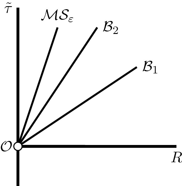
The key idea is to separate the sonic window $[x_{\text{min}},x_{\text{max}}]$ into the sets of sonic points $x_{\ast }$ that launch solutions $W(·;x_{\ast })$ which either stay above the Friedmann value $W_F=\frac{1}{3}$ on its maximum interval of existence $(s(x_{\ast }),x_{\ast }]$ or cross it, see Figure 1. This motivates the following definition.

Fig. 1.

Schematic depiction of the shooting argument. Here $x_{\ast 1}\in {\mathcal{X}}_{>\frac{1}{3}}$, $x_{\ast 2}\in {\mathcal{X}}_{\frac{1}{3}}$. The critical point ${\overline{x}}_{\ast }$ is obtained by sliding to the left in ${\mathcal{X}}_{\frac{1}{3}}$ until we reach the boundary of its first connected component X

Definition 2.2

(${\mathcal{X}}_{>\frac{1}{3}}$, ${\mathcal{X}}_{\frac{1}{3}}$, ${\mathcal{X}}_{<\frac{1}{3}}$, and X) Let ${\epsilon }_0>0$ be a small constant introduced in Section 2.2 (see also Theorem 4.18). For any $\epsilon \in (0,{\epsilon }_0]$ and $x_{\ast }\in [x_{\text{min}},x_{\text{max}}]$ we consider the associated RLP-type solution $(D(·;x_{\ast }),W(·;x_{\ast }))$. We introduce the sets

$$\begin{array}{cc}\hfill {\mathcal{X}}_{>\frac{1}{3}}& :=\left\{x_{\ast },\in ,[x_{\text{min}},x_{\text{max}}],,|,\underset{x\in (s(x_{\ast }),x_{\ast })}{inf},W,(x;x_{\ast }),>,\frac{1}{3}\right\},\hfill \end{array}$$ 2.44

$$\begin{array}{cc}\hfill {\mathcal{X}}_{\frac{1}{3}}& :=\left\{x_{\ast },\in ,[x_{\text{min}},x_{\text{max}}],,|,,\exists ,,x,\in ,(s(x_{\ast }),x_{\ast }),,\text{such that},,W,(x;x_{\ast }),=,\frac{1}{3}\right\},\hfill \end{array}$$ 2.45

$$\begin{array}{cc}\hfill {\mathcal{X}}_{<\frac{1}{3}}& :=\left\{x_{\ast },\in ,[x_{\text{min}},x_{\text{max}}],,|,W,(x;x_{\ast }),>,\frac{1}{3},,,\text{for all},,,x,\in ,(s(x_{\ast }),x_{\ast }),,\text{and},,\underset{x\in (s(x_{\ast }),x_{\ast })}{inf},W,(x;x_{\ast }),\le ,\frac{1}{3}\right\}.\hfill \end{array}$$ 2.46

Finally, we introduce the fundamental set $X\subset {\mathcal{X}}_{\frac{1}{3}}$ given by

$$\begin{array}{c}\hfill X:=\left\{x_{\ast },\in ,[x_{\text{min}},x_{\text{max}}],,|,,{\tilde{x}}_{\ast },\in ,{\mathcal{X}}_{\frac{1}{3}},,,\text{for all},,,{\tilde{x}}_{\ast },\in ,[x_{\ast },x_{\text{max}}]\right\}.\end{array}$$ 2.47

The basic observation is that solutions that correspond to the set ${\mathcal{X}}_{\frac{1}{3}}$ have the property that once they take on value $\frac{1}{3}$, they never go back up above it. This is a nonlinear invariance of the flow, which guides our shooting argument idea. It is possible to show that both sets ${\mathcal{X}}_{>\frac{1}{3}}$ and ${\mathcal{X}}_{\frac{1}{3}}$ are non-empty. In Lemma 5.9 we show that $x_{\text{min}}\in {\mathcal{X}}_{>\frac{1}{3}}$ and that for some $\kappa >0$, $(x_{\text{max}}-\kappa ,x_{\text{max}}]\subset {\mathcal{X}}_{\frac{1}{3}}$. Intuitively, we then slide down $x_{\ast }$ starting from $x_{\text{max}}$, until we reach the first value of $x_{\ast }$ that does not belong to ${\mathcal{X}}_{\frac{1}{3}}$, i.e. we let

$$\begin{array}{c}\hfill {\overline{x}}_{\ast }:=\underset{x_{\ast }\in X}{inf}{x}_{\ast },\end{array}$$ 2.48

see Figure 1. This is the candidate for the value of $x_{\ast }$ which gives a real-analytic solution on $[0,{\overline{x}}_{\ast }]$. Using the nonlinear invariances of the flow and its continuity properties, in Proposition 5.15, we show that the solution $(D(·;{\overline{x}}_{\ast }),W(·,{\overline{x}}_{\ast }))$ exists on the semi-open interval $(0,{\overline{x}}_{\ast }]$.

To show that the solution is indeed analytic all the way to $x=0$, $W(0;{\overline{x}}_{\ast })=\frac{1}{3}$, and $D(0;{\overline{x}}_{\ast })>\frac{1}{3}$, we adapt the strategy developed for the classical LP solution in [15]. Using the method of upper and lower solutions (Definition 5.23), we show that there exists a choice of $D_0>\frac{1}{3}$ such that the solution $(D(·;{\overline{x}}_{\ast }),W(·,{\overline{x}}_{\ast }))$ coincides with a unique real analytic solution to (2.35)–(2.36), with data $D(0)=D_0$, $W(0)=\frac{1}{3}$, solving from $x=0$ to the right. Detailed account of this strategy is contained in Sections 5.3–5.4. Finally, combining the above results we can prove the central statement of Section 5:

Theorem 2.3

There exists an ${\epsilon }_0>0$ sufficiently small, such that for any $0<\epsilon \le {\epsilon }_0$, the solution of RLP-type to (2.35)–(2.36) launched at ${\overline{x}}_{\ast }$ (defined by (2.48)) extends (to the left) to the closed interval $[0,{\overline{x}}_{\ast }]$, is real analytic, and satisfies $W(0;{\overline{x}}_{\ast })=\frac{1}{3}$, $D(0;{\overline{x}}_{\ast })>\frac{1}{3}$.

This theorem is formally proved at the very end of Section 5.4.

The Far-Field Connection (Section 6)

By contrast to establishing the existence of the Friedmann connection in Section 5, we show that for any choice of $x_{\ast }$ in our sonic window $[x_{\text{min}},x_{\text{max}}]$, there exists a global solution to the right, i.e. we prove the following theorem:

Theorem 2.4

Let $x_{\ast }\in [x_{\text{min}},x_{\text{max}}]$. There exists an $0<{\epsilon }_0\ll 1$ such that the unique RLP-type solution $(W,D)$ exists globally to the right for all $\epsilon \in (0,{\epsilon }_0]$.

The proof relies on a careful study of nonlinear invariances of the flow, and once again the monotonicity properties encoded in Lemma 3.7 play a critical role in our proof. This is highlighted in Lemma 6.3, which allows us to propagate the negativity of the sonic denominator B to the right of the sonic point. Importantly, we may now let $x_{\ast }={\overline{x}}_{\ast }$ defined in (2.48) to obtain a real-analytic RLP-type solution defined globally on $[0,\infty )$. As it turns out, the obtained spacetime is not maximally extended, and to address this issue we need to understand the asymptotic behaviour of our solutions as $x\to \infty$.

In Lemma 6.5 we show that solutions from Theorem 2.4 honour the asymptotic behaviour

$$\begin{array}{c}\hfill \underset{x\to \infty }{lim}W(x;x_{\ast })=1,\underset{x\to \infty }{lim}\left[D,(x;x_{\ast }),x^{\frac{2}{1+\eta }}\right]>0;\end{array}$$ 2.49

hence the name far-field connection, see (2.39). This is however not enough for the purposes of extending the solution beyond $x=\infty$, as we also need sharp asymptotic behaviour of the relative velocity W. Working with the nonlinear flow (2.35)–(2.36), in Proposition 6.8 we show that the leading order behaviour of W is given by the relation

$$\begin{array}{c}\hfill 1-W{\asymp }_{x\to \infty }{x}^{-\frac{1}{1+\eta }}.\end{array}$$ 2.50

Maximal Analytic Extension (Section 7)

Asymptotic relations (2.49)–(2.50) suggest that our unknowns are asymptotically “regular" only if thought of as functions of $x^{-\frac{1}{1+\eta }}$. In fact, it turns out to be more convenient to interpret this in the original comoving selfsimilar variable y, see (2.25). Due to (2.49) and (2.32)–(2.33), it is easy to see that asymptotically

$$\begin{array}{c}\hfill x{\asymp }_{x\to \infty }y.\end{array}$$ 2.51

Moreover, by (2.49) and (2.34), we have $\mathbf{d}(y){\asymp }_{y\to \infty }{y}^{-\frac{2}{1+\eta }}$. Furthermore by (3.101) we have the relation

$$\begin{array}{c}\hfill e^{2\mu }=\frac{1}{{(1+\epsilon )}^2}{\mathrm{\Sigma }}^{-\frac{\eta }{1+\eta }}=\frac{1}{{(1+\epsilon )}^2}{\mathbf{d}}^{-\eta }.\end{array}$$ 2.52

As a consequence of (2.49) we then conclude that

$$\begin{array}{c}\hfill e^{2\mu }{\asymp }_{y\to \infty }{y}^{\frac{4\epsilon }{1+\epsilon }},\end{array}$$ 2.53

which implies that the metric g given by (2.7) becomes singular as $y\to \infty$ (or equivalently $x\to \infty$). In Section 7 we show that this is merely a coordinate singularity, and the spacetime extends smoothly (in fact analytically in a suitable choice of coordinates) across the surface $\{(\tau \equiv 0,R)|R>0\}$.

Motivated by the above considerations, we switch to an adapted comoving chart $(\tilde{\tau },R)$, defined through

$$\begin{array}{c}\hfill \tilde{\tau }(\tau ,R)=-{\epsilon }^{-\frac{\epsilon }{1+\epsilon }}{R}^{\frac{2\epsilon }{1+\epsilon }}{(-\tau )}^{\frac{1-\epsilon }{1+\epsilon }},\tau <0,R>0.\end{array}$$ 2.54

We introduce the selfsimilar variable

$$\begin{array}{c}\hfill Y:=\frac{-\sqrt{\epsilon }\tilde{\tau }}{R},\end{array}$$ 2.55

which is then easily checked to be equivalent to the change of variables

$$\begin{array}{c}\hfill Y=y^{-\frac{1}{1+\eta }},y=Y^{-1-\eta },\end{array}$$ 2.56

where we recall $\eta =\eta (\epsilon )=\frac{2\epsilon }{1-\epsilon }$. To formulate the extension problem, it is natural to define the new variables

$$\begin{array}{c}\hfill \chi (Y):=\mathit{\chi }(y),d(Y):=\mathbf{d}(y),w(Y):=\mathbf{w}(y),\end{array}$$ 2.57

where we recall the fundamental variables $\mathbf{d},\mathbf{w},\mathit{\chi }$ from (2.26)–(2.28). Note that by (2.28) and (2.56) we have $\chi (Y)=Y^{1+\eta }\tilde{r}(y)$. It is shown in Lemma 7.1 that the original system (2.29)–(2.30) in the new variables reads

$$\begin{array}{cc}\hfill d^{\prime }& =\frac{2{\chi }^2}{Y}\frac{d{(w+\epsilon )}^2(d-w)}{\mathcal{C}},\hfill \end{array}$$ 2.58

$$\begin{array}{cc}\hfill w^{\prime }& =-\frac{(w+\epsilon )(1-3w)}{(1-\epsilon )Y}-\frac{2(1+\epsilon ){\chi }^2}{(1-\epsilon )Y}\frac{w{(w+\epsilon )}^2(d-w)}{\mathcal{C}},\hfill \end{array}$$ 2.59

$$\begin{array}{cc}\hfill {\chi }^{\prime }& =\frac{1-w}{(1-\epsilon )Y}\chi ,\hfill \end{array}$$ 2.60

where

$$\begin{array}{c}\hfill \mathcal{C}:={\left(d,Y^{-2}\right)}^{-\eta }{Y}^2-{\chi }^2\left[{(w+\epsilon )}^2,-,\epsilon ,{(w-1)}^2,+,4,\epsilon ,w,d\right].\end{array}$$ 2.61

The first main result of Section 7 is Theorem 7.4, where we prove the local existence of a real analytic solution in an open neighbourhood of $Y=0$, which provides the local extension of the solution from $Y=0^{+}$ to $Y=0^{-}$. Initial data at $Y=0$ are read off from the asymptotic behaviour (2.49)–(2.50), see Remark 7.2. The most important result of the section is the maximal extension theorem of the solution to the negative Y-s:

Theorem 2.5

(Maximal extension) There exists an $0<{\epsilon }_0\ll 1$ sufficiently small such that for any $\epsilon \in (0,{\epsilon }_0]$ there exists a $Y^{\text{ms}}<0$ such that the unique solution to the initial value problem (2.58)–(2.60) exists on the interval $(Y^{\text{ms}},0]$, and

$$\begin{array}{cc}& \underset{Y\to {(Y^{\text{ms}})}^{-}}{lim}w(Y)=\underset{Y\to {(Y^{\text{ms}})}^{-}}{lim}d(Y)=\infty ,\hfill \end{array}$$ 2.62

$$\begin{array}{cc}& \chi (Y)>0,Y\in (Y^{\text{ms}},0],\hfill \end{array}$$ 2.63

$$\begin{array}{cc}& \underset{Y\to {(Y^{\text{ms}})}^{-}}{lim}\chi (Y)=0.\hfill \end{array}$$ 2.64

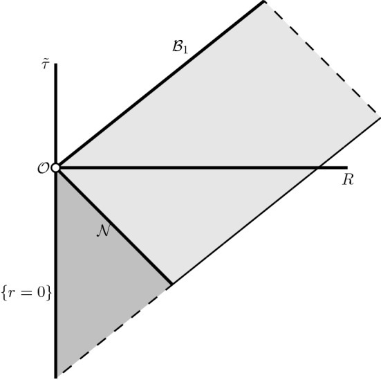
Fig. 2.

Schematic depiction of the behaviour of $\chi (Y)$ and $w(Y)$ in the maximal extension. As Y approaches $Y^{\text{ms}}$ from the right, $\chi$ approaches 0 and $w$ blows up to $\infty$

We see from the statement of the theorem that the maximal extension is characterised by the simultaneous blow-up of $w,d,$ and $\frac{1}{\chi }$ at the terminal point $Y^{\text{ms}}$. By (2.55), in the adapted comoving chart, the point $Y^{\text{ms}}$ coincides with the hypersurface

$$\begin{array}{c}\hfill \mathcal{M}{\mathcal{S}}_{\epsilon }:=\left\{(\tilde{\tau },R),,|,\tilde{\tau },=,\frac{1}{\sqrt{\epsilon }},|Y^{\text{ms}}|,R\right\}\backslash \{(0,0)\},\end{array}$$

which we refer to as the massive singularity, following the terminology in [28]. The proof of Theorem 2.5 relies on a careful understanding of nonlinear invariances associated with the dynamical system (2.58)–(2.60) and the key dynamic “sandwich" bound

$$\begin{array}{c}\hfill 1\lesssim \frac{d}{w}<1,\text{for}Y<Y_0<0,\end{array}$$

where $Y_0<0$ is small. This is shown in Lemma 7.9. The blow-up proof finally follows from a Ricatti-type ordinary differential inequality for the relative velocity $w$.

In Section 7.4 we compute the sharp asymptotics of $w,d,$ and $\chi$ on approach to the massive singularity $Y^{\text{ms}}$. This result is stated in Proposition 7.16, which is later crucially used in the study of the causal structure of such a maximally extended solution, where it is in particular shown that the spacetime curvature blows up on approach to the massive singularity.

Remark 2.6

The maximal selfsimilar extension makes sense in the Newtonian limit $\epsilon \to 0$, which is one of the key observations of Ori and Piran [28]. Our proof of Theorem 2.5 easily extends to the simpler case $\epsilon =0$, which in particular shows that the LP-solutions constructed in [15] have a natural maximal extension in the Lagrangian (comoving) coordinates.

The RLP-Spacetime and Its Causal Structure (Section 8)

As a consequence of Theorems 2.3, 2.4, and 2.5, we can now formally introduce the exactly selfsimilar solution of the Einstein-Euler system by patching the solutions in the subsonic region $x\in [0,{\overline{x}}_{\ast }]$, the supersonic region $x\in [{\overline{x}}_{\ast },\infty )$, and the extended region $Y\in (Y^{\text{ms}},0]$. Following Ori and Piran [28], we call this spacetime the relativistic Larson-Penston (RLP) solution3.

Definition 2.7

($g_{\text{RLP},\epsilon }$-metric) We refer to the 1-parameter family of spherically symmetric selfsimilar spacetimes $({\mathcal{M}}_{\text{RLP},\epsilon },g_{\text{RLP},\epsilon })$ constructed above as the relativistic Larson-Penston spacetimes. In the adapted comoving coordinates $(\tilde{\tau },R)$ the metric takes the form

$$\begin{array}{cc}\hfill g_{\text{RLP},\epsilon }& =-e^{2\tilde{\mu }}d{\tilde{\tau }}^2-\frac{4\sqrt{\epsilon }}{1+\epsilon }Y{e}^{2\tilde{\mu }}d\tilde{\tau }dR+\left(e^{2\tilde{\lambda }},-,\frac{4\epsilon }{{(1+\epsilon )}^2},Y^2,e^{2\tilde{\mu }}\right)d{R}^2+r^2\gamma ,\hfill \end{array}$$ 2.65

where the metric coefficients are defined on the connected component of the $(\tilde{\tau },R)$ coordinate plane given by

$$\begin{array}{c}\hfill {\tilde{\mathcal{D}}}_{\text{RLP},\epsilon }:=\left\{(\tilde{\tau },R),,|,,R,>,0,,,,Y,\in ,(Y^{\text{ms}},\infty )\right\}.\end{array}$$ 2.66

Here

$$\begin{array}{c}\hfill r(\tilde{\tau },R)=\chi (Y)R,\tilde{\mu }(\tilde{\tau },R)=\tilde{\mu }(Y),\tilde{\lambda }(\tilde{\tau },R)=\tilde{\lambda }(Y),\end{array}$$ 2.67

where $Y=-\frac{\sqrt{\epsilon }\tilde{\tau }}{R},$

$$\begin{array}{c}\hfill e^{2\tilde{\mu }(Y)}=\frac{{(1+\epsilon )}^2}{{(1-\epsilon )}^2}{Y}^{2\eta }{e}^{2\mu (y)},y>0,\end{array}$$ 2.68

and

$$\begin{array}{c}\hfill e^{2\tilde{\lambda }(Y)}=e^{2\lambda (y)},y>0.\end{array}$$ 2.69

Metric coefficients $\tilde{\mu }(Y),\tilde{\lambda }(Y)$ for $Y\le 0$ are then defined by expressing them as appropriate functions of $d,w,\chi$ and extending to $Y\le 0$, see Proposition 7.16.

The RLP-spacetime in the original comoving coordinates. In the original comoving coordinates $(\tau ,R)$, the metric takes the form

$$\begin{array}{cc}\hfill g_{\text{RLP},\epsilon }& =-e^{2\mu }d{\tau }^2+e^{2\lambda }d{R}^2+r^2\gamma .\hfill \end{array}$$ 2.70

It is clear from (2.53) that the metric (2.70) becomes singular across the surface $\tau =0$ (equivalently $y=\infty$). Nevertheless, away from this surface (i.e. when $\tau >0$ and $\tau <0$) we can keep using comoving coordinates, whereby we define

$$\begin{array}{c}\hfill \tau ={|Y|}^{\eta }\tilde{\tau },\tilde{\tau }>0,\end{array}$$ 2.71

where we recall (2.55). Therefore the metric coefficients are defined on the union of the connected components of the $(\tau ,R)$ coordinate plane given by

$$\begin{array}{c}\hfill {\mathcal{D}}_{\text{RLP},\epsilon }:=\left\{(,\tau ,,,R,),\in ,(,-,\infty ,,,0,),\times ,(,0,,,\infty ,)\right\}\cup \left\{(\tau ,R),\in ,(0,\infty ),\times ,(0,\infty ),,|,,y,\in ,(-\infty ,y^{\text{ms}})\right\},\end{array}$$ 2.72

where

$$\begin{array}{c}\hfill y^{\text{ms}}:=-{|Y^{\text{ms}}|}^{-(1+\eta )}.\end{array}$$

Here

$$\begin{array}{c}\hfill r(\tau ,R)=-\sqrt{\epsilon }\tau \tilde{r}(y),\mu (\tau ,R)=\mu (y),\lambda (\tau ,R)=\lambda (y),\text{for}\tau <0,\end{array}$$

and

$$\begin{array}{c}\hfill r=-\sqrt{\epsilon }\tau \tilde{r}(y),\tilde{r}(y)=\mathit{\chi }(y)y,y=\frac{R}{-\sqrt{\epsilon }\tau }=-{|Y|}^{-1-\eta },\text{for}\tau >0,\end{array}$$

where $\mathit{\chi }(y)=\chi (Y)$, $y<0$.

Remark 2.8

It is of interest to understand the leading order asymptotic behaviour of the radius $\tilde{r}$ as a function of the comoving selfsimilar variable y. It follows from (2.34) and the boundary condition $W(0)=\frac{1}{3}$ that ${lim}_{y\to 0^{+}}\mathbf{w}(y)=\frac{1}{3}$. Therefore, using (2.33) it is easy to see that the leading order behaviour of $\tilde{r}(y)$ at $y=0$ is of the form

$$\begin{array}{c}\hfill \tilde{r}(y)={\tilde{r}}_0{y}^{\frac{1+3\epsilon }{3(1+\epsilon )}}+o_{y\to 0^{+}}(y^{\frac{1+3\epsilon }{3(1+\epsilon )}}),{\tilde{r}}^{\prime }(y){\asymp }_{y\to 0^{+}}{y}^{-\frac{2}{3(1+\epsilon )}},\end{array}$$ 2.73

for some ${\tilde{r}}_0>0$. It follows in particular that $y\mapsto \tilde{r}(y)$ is only $C^{0,\frac{1+3\epsilon }{3(1+\epsilon )}}$ at $y=0$. The selfsimilar reduction of the constraint equation (2.15) reads ${\tilde{r}}^{\prime 2}{e}^{-2\lambda }=1+\epsilon V^2-\frac{2}{3}\epsilon \tilde{G}{\tilde{r}}^2$ (see (3.95)). Using this and (2.73), it then follows

$$\begin{array}{c}\hfill e^{\lambda (y)}{\asymp }_{y\to 0^{+}}{\tilde{r}}^{\prime }(y){\to }_{y\to 0^{+}}\infty ,\end{array}$$ 2.74

which shows that the metric g (2.7) is singular at $y=0$.

This singularity is not geometric, but instead caused by the Friedmann-like behaviour of the relative velocity W at $y=0$, see (2.40). It captures an important difference between the comoving and the Schwarzschild coordinates at the centre of symmetry $\{(\tau ,R)|\tau <0,R=0\}$. It can be checked that the space-time is regular at the centre of symmetry by switching to the $(\tau ,r)$ coordinate. The same phenomenon occurs in the Newtonian setting, where it can be shown that the map $\mathit{\chi }=\frac{\tilde{r}}{y}$ associated with the LP-solution is exactly $C^{0,\frac{1}{3}}$ and therefore $\mathit{\chi }$ is not smooth at the labelling origin $y=0$.

Remark 2.9

Note that the trace of $T_{\mu \nu }$ is easily evaluated

$$\begin{array}{c}\hfill g^{\mu \nu }{T}_{\mu \nu }=(\rho +p)g^{\mu \nu }{u}_{\mu }{u}_{\nu }+4p=-\rho +3p=-(1-3\epsilon )\rho .\end{array}$$

On the other hand, the trace of the left-hand side of (1.1) is exactly $-\mathcal{R}$, and therefore the Ricci scalar of any classical solution of (1.1)–(1.5) satisfies the relation

$$\begin{array}{c}\hfill \mathcal{R}=(1-3\epsilon )\rho .\end{array}$$ 2.75

This relation also implies that the blow-up of the Ricci scalar is equivalent to the blow up of the mass-energy density when $\epsilon \ne \frac{1}{3}$.

Remark 2.10

In Christodolou’s work [6], across the boundary of the backward light cone $\mathcal{N}$ emanating from the first singularity, the selfsimilar solution has finite regularity (measured in the Hölder class). This is to be contrasted with the RLP solution which remains real analytic across both characteristic cones - the sonic line and the light cone.

The Outgoing Null-Geodesic

The maximally extended RLP spacetime constructed above has two singular boundary components - the scaling origin $\mathcal{O}$ and the massive singularity $\mathcal{M}{\mathcal{S}}_{\epsilon }$ introduced in Section 2.5, see Figure 3. They are very different in nature, as the density (and the curvature components) blow up at two distinct rates.

Fig. 3.

Schematic depiction of the outgoing null-geodesics ${\mathcal{B}}_1$, ${\mathcal{B}}_2$, and the massive singularity $\mathcal{M}{\mathcal{S}}_{\epsilon }$

The main result of Section 8 states that there exist an outgoing radial null-geodesic (RNG) emanating from the scaling origin $\mathcal{O}$ and reaching infinity. Following Ori and Piran we look for a so-called simple RNG:

Definition 2.11

(Simple radial null-geodesics) An RNG of the form

$$\begin{array}{c}\hfill R(\tilde{\tau })=\sigma \tilde{\tau },\sigma \in \mathbb{R}\backslash \{0\},\end{array}$$ 2.76

is called a simple radial null-geodesic (simple RNG).

Then the key result we prove is the following theorem.

Theorem 2.12

(Existence of global outgoing simple RNG-s) There exists an $0<{\epsilon }_0\ll 1$ sufficiently small so that for any $\epsilon \in (0,{\epsilon }_0]$ there exist at least two and at most finitely many outgoing simple RNG-s emanating out of the singularity (0, 0). In other words, there exist

$$\begin{array}{c}\hfill Y^{\text{ms}}<Y_n<\cdots Y_1<0,n\ge 2,\end{array}$$ 2.77

so that the associated simple RNG-s are given by

$$\begin{array}{c}\hfill {\mathcal{B}}_i:=\{(\tilde{\tau },R)\in {\mathcal{M}}_{\text{RLP},\epsilon }|\frac{-\sqrt{\epsilon }\tilde{\tau }}{R}=Y_i\},i=1,\cdots n.\end{array}$$ 2.78

The proof relies on a beautiful idea of Ori and Piran [28], which we make rigorous. Namely, one can show that the slopes of outgoing simple RNG-s must correspond to roots of a certain real-analytic function, see Lemma 8.2. Using the sharp asymptotic behaviour of the metric coefficients, brought about through our analysis in Sections 6–7, we can prove that this function converges to negative values at $Y=0$ and $Y=Y^{\text{ms}}$. On the other hand, by the local existence theory for the ODE-system (2.58)–(2.60), we can also ascertain the function in question peaks above 0 for a $Y_0\in (Y^{\text{ms}},0)$. Therefore, by the intermediate value theorem, we conclude the proof of Theorem 2.12, see Section 8, immediately after Proposition 8.4.

Informally, the null-hypersurface ${\mathcal{B}}_1$ is the “first" outgoing null-curve emanating from the singular scaling origin and reaching the infinity. It is easy to see that r grows to $+\infty$ along ${\mathcal{B}}_1$. Since the spacetime is not asymptotically flat, we perform a suitable truncation in Section 9 in order to interpret $\mathcal{O}$ as a naked singularity.

The maximal extension we construct is unique only if we insist on it being selfsimilar, otherwise there could exist other extensions in the causal future of $\mathcal{O}$. Nevertheless, in our analysis the role of the massive singularity $\mathcal{M}{\mathcal{S}}_{\epsilon }$ is important, as we use the sharp blow-up asymptotics of our unknowns to run the intermediate value theorem-argument above. Conceptually, $\mathcal{M}{\mathcal{S}}_{\epsilon }$ has a natural Newtonian limit as $\epsilon \to 0$, see Remark 2.6, which makes it a useful object for our analysis.

In the remainder of Section 8 we give a detailed account of radial null-geodesics, showing in particular that there is a unique ingoing null-geodesic $\mathcal{N}$ emanating from the scaling origin to the past, see Figure 4. This is the boundary of the backward light cone “emanating" from the scaling origin. Following the terminology in [6], it splits the spacetime into the exterior region (in the future of $\mathcal{N}$) and the interior region (in the past of $\mathcal{N}$), see Definition 8.6 and Figure 5. Moreover, the sonic line is contained strictly in the interior region. The complete analysis of nonradial null-geodesics is given in Appendix B.

Fig. 4.

Schematic depiction of the ingoing null-curve $\mathcal{N}$ and the sonic line. The spacetime is smooth across both surfaces

Fig. 5.

Schematic depiction of the interior (dark grey) and the exterior (light grey) region, see Definition 8.6

Double Null Gauge, Asymptotic Flattening, and Naked Singularities (Section 9)

The final step in the proof of Theorem 1.2 is to truncate the profile away from the scaling origin $\mathcal{O}$ and glue it to the already constructed selfsimilar solution. To do that we set up this problem in the double-null gauge:

$$\begin{array}{c}\hfill g=-{\mathrm{\Omega }}^{2}dpdq+r^2\gamma ,\end{array}$$ 2.79

where $p=\text{const.}$ corresponds to outgoing null-surfaces and $q=\text{const.}$ to the ingoing null-surfaces. A similar procedure for the scalar field model was implemented in [6], however due to the complications associated with the Euler evolution, a mere cut-off argument connecting the “inner region" to pure vacuum as we approach null-infinity is hard to do. Instead, we carefully design function spaces that capture the asymptotic decay of the fluid density toward future null-infinity in a way that is both consistent with the asymptotic flatness, and can be propagated dynamically.

Formulation of the Problem in Double-Null Gauge

In addition to the unknowns associated with the fluid, the metric unknowns are the conformal factor $\mathrm{\Omega }=\mathrm{\Omega }(p,q)$ and the areal radius $r=r(p,q)$. Clearly,

$$\begin{array}{c}\hfill g_{\mathit{pp}}=g_{\mathit{qq}}=0,g_{\mathit{pq}}=-\frac{1}{2}{\mathrm{\Omega }}^2,g^{\mathit{pq}}=-2{\mathrm{\Omega }}^{-2}.\end{array}$$ 2.80

Let $u=(u^p,u^q,0,0)$ be the components of the velocity 4-vector u in the frame $\{{\partial }_p,{\partial }_q,E_2,E_3\}$, where $\{E_A\}$, $A=2,3$, describe the generators of some local coordinates on ${\mathbb{S}}^2$. We have $g({\partial }_p,E_A)=g({\partial }_q,E_A)=0$, $A=2,3$. The normalisation condition (1.3) in the double-null gauge reads

$$\begin{array}{c}\hfill -1=g^{\mu \nu }{u}_{\mu }{u}_{\nu }=g^{\mathit{pq}}{u}_p{u}_q=-4{\mathrm{\Omega }}^{-2}{u}_p{u}_q,\end{array}$$ 2.81

which therefore equivalently reads

$$\begin{array}{c}\hfill u_p{u}_q=\frac{1}{4}{\mathrm{\Omega }}^2,u^p{u}^q={\mathrm{\Omega }}^{-2}.\end{array}$$ 2.82

Lemma 2.13

(Einstein-Euler system in double-null gauge) In the double-null gauge (2.79), the Einstein field equations take the form

$$\begin{array}{cc}\hfill {\partial }_p{\partial }_{q}r& =-\frac{{\mathrm{\Omega }}^2}{4r}-\frac{1}{r}{\partial }_{p}r{\partial }_{q}r+\pi r{\mathrm{\Omega }}^4{T}^{\mathit{pq}},\hfill \end{array}$$ 2.83

$$\begin{array}{cc}\hfill {\partial }_p{\partial }_{q}log\mathrm{\Omega }& =-(1+\eta )\pi {\mathrm{\Omega }}^4{T}^{\mathit{pq}}+\frac{{\mathrm{\Omega }}^2}{4r^2}+\frac{1}{r^2}{\partial }_{p}r{\partial }_{q}r,\hfill \end{array}$$ 2.84

$$\begin{array}{cc}\hfill {\partial }_q\left({\mathrm{\Omega }}^{-2},{\partial }_q,r\right)& =-\pi r{\mathrm{\Omega }}^2{T}^{\mathit{pp}},\hfill \end{array}$$ 2.85

$$\begin{array}{cc}\hfill {\partial }_p\left({\mathrm{\Omega }}^{-2},{\partial }_p,r\right)& =-\pi r{\mathrm{\Omega }}^2{T}^{\mathit{qq}}.\hfill \end{array}$$ 2.86

Moreover, the components of the energy-momentum tensor satisfy

$$\begin{array}{cc}\hfill {\partial }_p({\mathrm{\Omega }}^4{r}^2{T}^{\mathit{pp}})+\frac{{\mathrm{\Omega }}^2}{r^{2\eta }}{\partial }_q({\mathrm{\Omega }}^2{r}^{2+2\eta }{T}^{\mathit{pq}})& =0,\hfill \end{array}$$ 2.87

$$\begin{array}{cc}\hfill {\partial }_p({\mathrm{\Omega }}^2{r}^{2+2\eta }{T}^{\mathit{pq}})+\frac{r^{2\eta }}{{\mathrm{\Omega }}^2}{\partial }_q({\mathrm{\Omega }}^4{r}^2{T}^{\mathit{qq}})& =0,\hfill \end{array}$$ 2.88

where the energy-momentum tensor is given by the formulas

$$\begin{array}{cc}& T^{\mathit{pp}}=(1+\epsilon )\rho {(u^p)}^2,T^{\mathit{qq}}=(1+\epsilon )\rho {(u^q)}^2,T^{\mathit{pq}}=(1-\epsilon )\rho {\mathrm{\Omega }}^{-2},\hfill \end{array}$$ 2.89

$$\begin{array}{cc}& T^{\mathit{AB}}=\epsilon \rho r^{-2}{\gamma }^{\mathit{AB}},T^{\mathit{pA}}=T^{\mathit{qA}}=0,A,B=2,3.\hfill \end{array}$$ 2.90

Moreover, its components are related through the algebraic relation

$$\begin{array}{c}\hfill T^{\mathit{pp}}{T}^{\mathit{qq}}={(1+\eta )}^2{(T^{\mathit{pq}})}^2.\end{array}$$ 2.91

Proof

The proof is a straightforward calculation and is given in Appendix C. $\square$

The Characteristic Cauchy Problem and Asymptotic Flattening

The idea is to choose a point $(p_0,q_0)$ in the exterior region (recall Figure 5) and solve the Einstein-Euler system in an infinite semi-rectangular domain (in the $(p,q)$-plane) $\mathcal{D}$ depicted in Figure 6. We normalise the choice of the double-null coordinates by making the outgoing curve ${\mathcal{B}}_1$ in the RLP-spacetime (see Figures 4–5) correspond to the $\{p=0\}$ level set, and the ingoing curve $\mathcal{N}$ (see Figure 5) to the $\{q=0\}$ level set. We have the freedom to prescribe the data along the ingoing boundary $\underset{\_}{\mathcal{C}}=\{(p,q)|p\in [p_0,0],q=q_0\}$ and the outgoing boundary $\mathcal{C}=\{(p,q)|p=p_0,q\ge q_0\}$. On $\underset{\_}{\mathcal{C}}$ we demand that data be given by the restriction of the selfsimilar RLP solution to $\underset{\_}{\mathcal{C}}$, and on the outgoing piece we make the data exactly selfsimilar on a subinterval $q\in [q_0,q_0+A_0]$ for some $A_0>0$. On the remaining part of the outgoing boundary $q\in [q_0+A_0,\infty )$, we prescribe asymptotically flat data.

Fig. 6.

The grey shaded area is the region $\mathcal{D}$, where the truncation of the selfsimilar profile takes place. Data are prescribed on the two characteristic surfaces $\mathcal{C}$ and $\underset{\_}{\mathcal{C}}$

The key result of Section 9 is Theorem 9.4, which states that the above described PDE is well-posed on $\mathcal{D}$, if we choose $|p_0|=\delta$ sufficiently small. We are not aware of such a well-posedness result for the Einstein-Euler system in the double-null gauge in the literature, and we therefore carefully develop the necessary theory. Precise statements are provided in Section 9.2. The idea is standard and relies on the method of characteristics. However, to make it work we rely on an effective “diagonalisation" of the Euler equations (2.87)–(2.88), which replaces these equations by two transport equations for the new unknowns $f^{+}$ and $f^{-}$, see Lemma 9.1. This change of variables highlights the role of the acoustic cone and allows us to track the acoustic domain of dependence by following the characteristics, see Figure 6. The analysis of the fluid characteristics is presented in Section 9.3. Various a priori bounds are given in Section 9.4. In Section 9.5 we finally introduce an iteration procedure and prove Theorem 9.4.

Formation of Naked Singularities: Proof of Theorem 1.2

Since the data on $\underset{\_}{\mathcal{C}}$ and the portion of $\mathcal{C}$ with $q_0\le q\le q_0+A_0$ agrees with the RLP-solution, the solution must, by the finite-speed of propagation, coincide with the exact RLP solution in the region ${\mathcal{D}}_{A_0}$ depicted in Figure 7. By uniqueness the solution extends smoothly (in fact analytically) to the exact RLP-solution in the past of $\underset{\_}{\mathcal{C}}$, all the way to the regular centre $\{r=R=0\}$.

Fig. 7.

The light grey shaded area is the region ${\mathcal{D}}_{A_0}$, where the truncated solution from Theorem 9.4 coincides with the exact selfsimilar solution

The future boundary of the maximal development is precisely the surface $\{p=0\}$, the Cauchy horizon for the new spacetime. The boundary of the null-cone corresponding to $\{p=p_0\}$ is complete, and we show in Section 9.6 that for any sequence of points $(p_0,q_n)$ with $q_n$ approaching infinity, the affine length of maximal future-oriented ingoing geodesics launched from $(p_0,q_n)$ and normalised so that the tangent vector corresponds to ${\partial }_p$, is bounded by a constant, uniformly-in-n. This shows that the future null-infinity is incomplete in the sense of [32, Definition 1.1], thus completing the proof of Theorem 1.2, see the Penrose diagram, Figure 8.

Fig. 8.

Penrose diagram of our spacetime with an incomplete future null-infinity

Radially Symmetric Einstein-Euler System in Comoving Coordinates

Selfsimilar Comoving Coordinates

We plug in (2.19)–(2.24) into (2.12)–(2.15) and obtain the selfsimilar formulation of the Einstein-Euler system:

$$\begin{array}{cc}\hfill 2\mathrm{\Sigma }+y{\mathrm{\Sigma }}^{\prime }(y)+(1+\epsilon )\mathrm{\Sigma }\left(\frac{V^{\prime }}{{\tilde{r}}^{\prime }},+,\frac{2V}{\tilde{r}}\right)e^{\mu }& =0,\hfill \end{array}$$ 3.92

$$\begin{array}{c}\hfill y{\lambda }^{\prime }(y)=e^{\mu }\frac{V^{\prime }}{{\tilde{r}}^{\prime }},\end{array}$$ 3.93

$$\begin{array}{cc}\hfill e^{-\mu }y{V}^{\prime }(y)+\frac{1}{1+\epsilon }\frac{{\tilde{r}}^{\prime }(y)e^{-2\lambda (y)}}{\mathrm{\Sigma }(y)}{\mathrm{\Sigma }}^{\prime }(y)+\tilde{r}\left(\frac{1}{3},\tilde{G},+,2,\epsilon ,\mathrm{\Sigma }\right)& =0,\hfill \end{array}$$ 3.94

$$\begin{array}{cc}\hfill {\tilde{r}}^{\prime 2}{e}^{-2\lambda }& =1+\epsilon V^2-\frac{2}{3}\epsilon \tilde{G}{\tilde{r}}^2.\hfill \end{array}$$ 3.95

Remark 3.1

Recall that the radial velocity $\mathcal{V}$ satisfies $\mathcal{V}=e^{-\mu }{\partial }_{\tau }r$ and therefore

$$\begin{array}{c}\hfill V=e^{-\mu }(-\tilde{r}+y{\tilde{r}}^{\prime }(y)).\end{array}$$ 3.96

From (3.92), (3.93), and (3.96) we obtain

$$\begin{array}{cc}\hfill 0& =2+y\frac{{\mathrm{\Sigma }}^{\prime }(y)}{\mathrm{\Sigma }(y)}+(1+\epsilon )\left(y,{\lambda }^{\prime },(y),+,2,\left(y,\frac{{\tilde{r}}^{\prime }(y)}{\tilde{r}(y)},-,1\right)\right)\hfill \end{array}$$

and therefore

$$\begin{array}{c}\hfill {\lambda }^{\prime }(y)=-\frac{1}{1+\epsilon }\left(\frac{{\mathrm{\Sigma }}^{\prime }}{\mathrm{\Sigma }},+,\frac{2}{y}\right)-2\left(\frac{{\tilde{r}}^{\prime }}{\tilde{r}},-,\frac{1}{y}\right).\end{array}$$ 3.97

For smooth solutions with strictly positive density $\mathrm{\Sigma }$, an explicit integration of the identity (3.97) gives the formula

$$\begin{array}{c}\hfill e^{\lambda }=\alpha {\mathrm{\Sigma }}^{-\frac{1}{1+\epsilon }}{y}^{\frac{2\epsilon }{1+\epsilon }}{\tilde{r}}^{-2},\end{array}$$ 3.98

for some constant $\alpha >0$.

Remark 3.2

(Gauge normalisation) From (2.16) we also obtain

$$\begin{array}{c}\hfill {\mu }^{\prime }(y)=-\frac{\epsilon }{1+\epsilon }\frac{{\mathrm{\Sigma }}^{\prime }(y)}{\mathrm{\Sigma }(y)}.\end{array}$$ 3.99

For any given $0<\epsilon <1$ we finally fix the remaining freedom in the problem by setting

$$\begin{array}{c}\hfill c=e^{2\mu (0)}\mathrm{\Sigma }{(0)}^{\frac{2\epsilon }{\epsilon +1}}=\frac{1}{{(1+\epsilon )}^2}.\end{array}$$ 3.100

Upon integrating (3.99) we obtain the identity

$$\begin{array}{c}\hfill e^{\mu (y)}=\frac{1}{1+\epsilon }\mathrm{\Sigma }{(y)}^{-\frac{\epsilon }{1+\epsilon }}.\end{array}$$ 3.101

Before we reduce the selfsimilar formulation (3.92)–(3.95) to a suitable $2\times 2$ nonautonomous ODE system, we first prove an auxiliary lemma.

Lemma 3.3

Let $(\mathrm{\Sigma },V,\lambda ,\mu )$ be a smooth solution to (3.92)–(3.95).

(a)

The following important relationship holds:

$$\begin{array}{c}\hfill \frac{\mathbf{w}+\epsilon }{1+\epsilon }=\frac{y{\tilde{r}}^{\prime }}{\tilde{r}},\end{array}$$ 3.102

with $\mathbf{w}$ defined by (2.27).

(b)

(Local expression for the mean density) The selfsimilar mean density $\tilde{G}$ defined by

$$\begin{array}{c}\hfill \tilde{G}(y)=\frac{6}{{\tilde{r}}^3}{\int }_0^y\mathrm{\Sigma }{\tilde{r}}^2{\tilde{r}}^{\prime }d\tilde{y}\end{array}$$ 3.103

satisfies the relation

$$\begin{array}{c}\hfill \tilde{G}=6\mathrm{\Sigma }\mathbf{w}.\end{array}$$ 3.104

(c)

The expression K defined by

$$\begin{array}{c}\hfill K:=-\frac{\mathbf{w}}{1+\epsilon }+e^{2\mu }\left(\frac{1}{6},\frac{(1+\epsilon )\tilde{G}}{\mathbf{w}+\epsilon },+,\frac{\epsilon (1+\epsilon )\mathrm{\Sigma }}{\mathbf{w}+\epsilon }\right).\end{array}$$ 3.105

satisfies the relation

$$\begin{array}{c}\hfill K=\frac{1}{1+\epsilon }\left(\mathbf{d},-,\mathbf{w}\right),\end{array}$$ 3.106

with $\mathbf{d}$ defined by (2.26).

(d)

The metric coefficient $e^{2\lambda }$ satisfies the formula

$$\begin{array}{c}\hfill e^{2\lambda }=\frac{{\tilde{r}}^2{(\mathbf{w}+\epsilon )}^2}{{(1+\epsilon )}^2{y}^2\left[1,+,\epsilon ,{\mathrm{\Sigma }}^{\frac{2\epsilon }{1+\epsilon }},{\tilde{r}}^2,{(\mathbf{w}-1)}^2,-,4,\epsilon ,\mathrm{\Sigma },\mathbf{w},{\tilde{r}}^2\right]}.\end{array}$$ 3.107

Proof

Proof of part (a). This is a trivial consequence of  (3.96) and (2.27).

Proof of part (b). After multiplying (3.92) by ${\tilde{r}}^2{\tilde{r}}^{\prime }$ we obtain

$$\begin{array}{cc}\hfill 0& =2\mathrm{\Sigma }{\tilde{r}}^2{\tilde{r}}^{\prime }+\underset{=\tilde{r}+V{e}^{\mu }}{\underbrace{y{\tilde{r}}^{\prime }}}{\tilde{r}}^2{\mathrm{\Sigma }}^{\prime }+(1+\epsilon )\mathrm{\Sigma }({\tilde{r}}^2{V}^{\prime }+2\tilde{r}{\tilde{r}}^{\prime }V)e^{\mu }\hfill \end{array}$$ 3.108

$$\begin{array}{cc}& =2\mathrm{\Sigma }{\tilde{r}}^2{\tilde{r}}^{\prime }+{\mathrm{\Sigma }}^{\prime }{\tilde{r}}^3+e^{\mu }{\mathrm{\Sigma }}^{\prime }{\tilde{r}}^{2}V+(1+\epsilon )e^{\mu }\mathrm{\Sigma }{({\tilde{r}}^{2}V)}^{\prime }\hfill \end{array}$$ 3.109

$$\begin{array}{cc}& =2\mathrm{\Sigma }{\tilde{r}}^2{\tilde{r}}^{\prime }+{\mathrm{\Sigma }}^{\prime }{\tilde{r}}^3+(1+\epsilon ){(e^{\mu }\mathrm{\Sigma }{\tilde{r}}^{2}V)}^{\prime }\hfill \end{array}$$ 3.110

where in the second line we used $y{\tilde{r}}^{\prime }=\tilde{r}+V{e}^{\mu }$ (which follows from (3.96)) and in the last line the identity

$$\begin{array}{c}\hfill {(\mathrm{\Sigma }{e}^{\mu })}^{\prime }={\mathrm{\Sigma }}^{\prime }{e}^{\mu }+\mathrm{\Sigma }{e}^{\mu }(-\frac{\epsilon }{1+\epsilon }\frac{{\mathrm{\Sigma }}^{\prime }}{\mathrm{\Sigma }})=\frac{1}{1+\epsilon }{\mathrm{\Sigma }}^{\prime }{e}^{\mu },\end{array}$$

which uses the field equation (3.99). After integrating over the interval [0, y] and integrating-by-parts, we obtain

$$\begin{array}{c}\hfill {\int }_0^y\mathrm{\Sigma }{\tilde{r}}^2{\tilde{r}}^{\prime }ds=\mathrm{\Sigma }{\tilde{r}}^2(\tilde{r}+(1+\epsilon )e^{\mu }V)=\mathrm{\Sigma }{\tilde{r}}^3\mathbf{w}\end{array}$$ 3.111

where we have used (2.27). Hence dividing by ${\tilde{r}}^3$ we obtain (3.104).

Proof of part (c). From (3.105) and (3.104) we immediately have

$$\begin{array}{c}\hfill K=(1+\epsilon )e^{2\mu }\mathrm{\Sigma }\frac{\mathbf{w}}{1+\epsilon }=\frac{1}{1+\epsilon }\left({\mathrm{\Sigma }}^{\frac{1-\epsilon }{1+\epsilon }},-,\mathbf{w}\right),\end{array}$$ 3.112

where we have used (3.101).

Proof of part (d). The formula is a simple consequence of (3.95), (3.96), and (3.104). $\square$

Proposition 3.4

(The ODE system in comoving selfsimilar coordinates) Let $(\mathrm{\Sigma },V,\lambda ,\mu )$ be a smooth solution to (3.92)–(3.95). Then the pair $(\mathbf{d},\mathbf{w})$ solves the system (2.29)–(2.30), where $\mathbf{d},\mathbf{w}$ are defined in (2.26)–(2.27).

Proof

A routine calculation starting from (3.92) and (3.94) (these can be thought of as the continuity and the momentum equation respectively) gives:

$$\begin{array}{cc}& \left(y,+,\epsilon ,\frac{y}{\mathbf{w}+\epsilon },(\mathbf{w}-1)\right){\mathrm{\Sigma }}^{\prime }+\frac{(1+\epsilon )\mathrm{\Sigma }y}{\mathbf{w}+\epsilon }{\mathbf{w}}^{\prime }-(1+3\epsilon )\mathrm{\Sigma }+3(\mathbf{w}+\epsilon )\mathrm{\Sigma }=0,\hfill \end{array}$$ 3.113

$$\begin{array}{cc}& e^{-2\mu }y\mathrm{\Sigma }{\mathbf{w}}^{\prime }+\frac{1}{1+\epsilon }\left(\epsilon ,e^{-2\mu },y,(\mathbf{w}-1),+,\frac{(\mathbf{w}+\epsilon )e^{-2\lambda }}{y}\right){\mathrm{\Sigma }}^{\prime }+e^{-2\mu }\mathrm{\Sigma }\frac{(\mathbf{w}+\epsilon )(\mathbf{w}-1)}{1+\epsilon }\hfill \\ \hfill & +(1+\epsilon )\left(\frac{1}{3},\mathrm{\Sigma },\tilde{G},+,2,\epsilon ,{\mathrm{\Sigma }}^2\right)=0.\hfill \end{array}$$ 3.114

We may rewrite (3.113)–(3.114) in the form

$$\begin{array}{cc}\hfill {\mathrm{\Sigma }}^{\prime }& =\frac{2y(1+\epsilon )\mathrm{\Sigma }}{y^2-e^{2\mu -2\lambda }}\left(-,\frac{\mathbf{w}}{1+\epsilon },+,e^{2\mu },\left(\frac{1}{6},\frac{(1+\epsilon )\tilde{G}}{\mathbf{w}+\epsilon },+,\frac{\epsilon (1+\epsilon )\mathrm{\Sigma }}{\mathbf{w}+\epsilon }\right)\right),\hfill \end{array}$$ 3.115

$$\begin{array}{cc}\hfill \frac{{\mathbf{w}}^{\prime }}{1+\epsilon }& =\frac{(\mathbf{w}+\epsilon )\left(1,-,3,\mathbf{w}\right)}{{(1+\epsilon )}^{2}y}-\frac{2y\mathbf{w}}{y^2-e^{2\mu -2\lambda }}\left(-,\frac{\mathbf{w}}{1+\epsilon },+,e^{2\mu },\left(\frac{1}{6},\frac{(1+\epsilon )\tilde{G}}{\mathbf{w}+\epsilon },+,\frac{\epsilon (1+\epsilon )\mathrm{\Sigma }}{\mathbf{w}+\epsilon }\right)\right).\hfill \end{array}$$ 3.116

With (3.105) in mind, equations (3.115)–(3.116) take the form

$$\begin{array}{cc}\hfill {\mathrm{\Sigma }}^{\prime }& =-\frac{2(1+\epsilon )\mathrm{\Sigma }K}{y(e^{2\mu -2\lambda }{y}^{-2}-1)},\hfill \end{array}$$ 3.117

$$\begin{array}{cc}\hfill {\mathbf{w}}^{\prime }& =\frac{(\mathbf{w}+\epsilon )(1-3\mathbf{w})}{(1+\epsilon )y}+\frac{2(1+\epsilon )\mathbf{w}K}{y(e^{2\mu -2\lambda }{y}^{-2}-1)},\hfill \end{array}$$ 3.118

where K is given by (3.105) and $\tilde{G}$ by (3.103). Equations (2.29)–(2.30) now follow from (2.26) and parts (b) and (c) of Lemma 3.3. $\square$

Selfsimilar Schwarzschild Coordinates

We recall the selfsimilar Schwarzschild coordinate introduced in (2.32).

Lemma 3.5

(Selfsimilar Schwarzschild formulation) Let $(\mathrm{\Sigma },\mathbf{w})$ be a smooth solution to (3.117)–(3.118). Then the variables $(D,W)$ defined by (2.34) solve the system (2.35)–(2.36), with B given by (2.37) and $\eta =\eta (\epsilon )=\frac{2\epsilon }{1-\epsilon }$.

Proof

With the above notation and Lemma 3.3 we have $K=\frac{1}{1+\epsilon }\left(D,-,W\right)$. It is straightforward to see that the system (3.117)–(3.118) transforms into

$$\begin{array}{cc}\hfill D^{\prime }& =-\frac{2(1-\epsilon )xD(W+\epsilon )(D-W)}{x^2{(W+\epsilon )}^2(e^{2\mu -2\lambda }{y}^{-2}-1)},\hfill \end{array}$$ 3.119

$$\begin{array}{cc}\hfill W^{\prime }& =\frac{1-3W}{x}+\frac{2(1+\epsilon )xW(W+\epsilon )(D-W)}{x^2{(W+\epsilon )}^2(e^{2\mu -2\lambda }{y}^{-2}-1)}.\hfill \end{array}$$ 3.120

From (2.33), the constraint equation (3.95), and (2.27)

$$\begin{array}{cc}\hfill \frac{{(W+\epsilon )}^2}{{(1+\epsilon )}^2}{x}^2{e}^{2\mu -2\lambda }{y}^{-2}& ={\tilde{r}}^{\prime 2}{e}^{2\mu -2\lambda }=e^{2\mu }(1+\epsilon V^2-\frac{2}{3}\epsilon \tilde{G}{\tilde{r}}^2)\hfill \\ \hfill & =e^{2\mu }\left(1,+,\epsilon ,e^{-2\mu },x^2,\frac{{(W-1)}^2}{{(1+\epsilon )}^2},-,4,\epsilon ,\mathrm{\Sigma },W,x^2\right),\hfill \end{array}$$ 3.121

where we have slightly abused notation by letting $\mathrm{\Sigma }(x)=\mathrm{\Sigma }(y)$. Therefore

$$\begin{array}{cc}\hfill & \frac{{(W+\epsilon )}^2}{{(1+\epsilon )}^2}{x}^2{e}^{2\mu -2\lambda }{y}^{-2}-\frac{{(W+\epsilon )}^2}{{(1+\epsilon )}^2}{x}^2=\frac{{\mathrm{\Sigma }}^{-\frac{2\epsilon }{1+\epsilon }}}{{(1+\epsilon )}^2}\hfill \\ \hfill & -\left[\frac{{(W+\epsilon )}^2}{{(1+\epsilon )}^2},-,\epsilon ,\frac{{(W-1)}^2}{{(1+\epsilon )}^2},+,\frac{4\epsilon }{{(1+\epsilon )}^2},{\mathrm{\Sigma }}^{\frac{1-\epsilon }{1+\epsilon }},W\right]x^2,\hfill \end{array}$$ 3.122

where we have used (3.101). Plugging this back into (3.119)–(3.119), the claim follows. $\square$

Lemma 3.6

(Algebraic structure of the sonic denominator B) Consider the denominator $B[x;D,W]$ defined in (2.37). We may factorise B in the form

$$\begin{array}{c}\hfill B[x;D,W]=(1-\epsilon )(J[x;D]-xW(x))(H[x;D]+xW(x)),\end{array}$$ 3.123

where

$$\begin{array}{cc}\hfill J[x;D]=J& :=-\frac{2\epsilon }{1-\epsilon }(1+D)x+\sqrt{\frac{4{\epsilon }^2}{{(1-\epsilon )}^2}{(1+D)}^2{x}^2+\epsilon x^2+\frac{D^{-\eta }}{1-\epsilon }},\hfill \end{array}$$ 3.124

$$\begin{array}{cc}\hfill H[x;D]=H& :=J[x;D]+\frac{4\epsilon }{1-\epsilon }(1+D)x.\hfill \end{array}$$ 3.125

Moreover,

$$\begin{array}{c}\hfill (1-\epsilon )JH=D^{-\eta }+\epsilon (1-\epsilon )x^2,\end{array}$$ 3.126

and

$$\begin{array}{c}\hfill J^{\prime }=\frac{-2\epsilon J(1+D)+\epsilon (1-\epsilon )x-(2\epsilon xJ+\frac{\epsilon }{1-\epsilon }{D}^{-\eta -1})D^{\prime }}{(1-\epsilon )J+2\epsilon x(1+D)}.\end{array}$$ 3.127

Proof

From (2.37) it is clear that we may view $B[x;D,W]$ as a quadratic polynomial in W:

$$\begin{array}{c}\hfill W^2+\frac{4\epsilon }{1-\epsilon }(1+D)W-\epsilon -\frac{x^{-2}{D}^{-\eta }}{1-\epsilon }=0.\end{array}$$

Solving for W, we obtain two roots, which when multiplied by x give

$$\begin{array}{c}\hfill x{W}_{\pm }=\frac{-2\epsilon x(1+D)\pm \sqrt{4{\epsilon }^2{x}^2{(1+D)}^2+(1-\epsilon )\left(\epsilon ,(1-\epsilon ),+,D^{-\eta }\right)}}{1-\epsilon }.\end{array}$$ 3.128

We now observe from (3.124)–(3.125) that the positive solution corresponds to $J[x;D]$ and the negative one to $-H[x;D]$. This in turn immediately gives (3.123). Property (3.126) is obvious from (3.124)–(3.125). Finally, to show (3.127) observe that $J$ solves

$$\begin{array}{c}\hfill (1-\epsilon )J^2+4\epsilon x(1+D)J-\epsilon (1-\epsilon )x^2-D^{-\eta }=0.\end{array}$$

We differentiate the above equality, regroup terms and obtain (3.127). $\square$

The Monotonicity Lemma

Controlling the sonic denominator B from below will be one of the central technical challenges in our analysis. From Lemma 3.6 it is clear that this can be accomplished by tracking the quantity $J[x;D]-xW(x)$. A related quantity, of fundamental importance in our analysis is given by

$$\begin{array}{c}\hfill f(x):=J[x;D]-xD.\end{array}$$ 3.129

The goal of the next lemma is to derive a first order ODE satisfied by f, assuming that we have a smooth solution to the system (2.35)–(2.36). This lemma will play a central role in our analysis.

Lemma 3.7

Let $(D,W)$ be a smooth solution to the selfsimilar Einstein-Euler system (2.35)–(2.36) on some interval $I\subset (0,\infty )$, and let f be given by (3.129). Then, the function f satisfies the ODE

$$\begin{array}{c}\hfill f^{\prime }(x)+a[x;D,W]f(x)=b[x;D,W],x\in I,\end{array}$$ 3.130

where

$$\begin{array}{c}\hfill a[x;D,W]=a_1[x;D,W]+a_2[x;D,W],b[x;D,W]=b_1[x;D,W]+\epsilon b_2[x;D,W]\end{array}$$

and

$$\begin{array}{cc}\hfill a_1[x;D,W]& =\left(\frac{2\epsilon xJ+\frac{\epsilon }{1-\epsilon }{D}^{-\eta -1}}{(1-\epsilon )J+2\epsilon x\left(1,+,D\right)},+,x\right)\frac{2(1-\epsilon )D\left(W,+,\epsilon \right)}{B}\hfill \\ \hfill & -2\epsilon \left(\frac{1}{1-\epsilon },\frac{D^{-\eta }}{x},+,(1-\epsilon ),x,+,(D+\epsilon ),f\right)Z^{-1};\hfill \end{array}$$ 3.131

$$\begin{array}{cc}\hfill a_2[x;D,W]& =2\epsilon \left[\left(J,-,x,W\right),\left(D,-,1\right),+,2,f,+,4,\epsilon ,x,+,x,D,\left(5,+,\epsilon \right)\right]Z^{-1};\hfill \end{array}$$ 3.132

$$\begin{array}{cc}\hfill b_1[x;D,W]& =\frac{D}{H+xW}(xW-J)+\epsilon (xW-J)Z^{-1}\left(x,\left(2,D^2,-,2,D,+,1,-,\epsilon \right)\right)\hfill \\ \hfill & \left(+,\frac{2}{(1-\epsilon )x},D^{-\eta }\right);\hfill \end{array}$$ 3.133

$$\begin{array}{cc}\hfill b_2[x,D,W]& =-2x^2\{D\left[D^2,+,(3+\epsilon ),D,-,(1-\epsilon )\right]\hfill \\ \hfill & +\epsilon \left[\frac{4}{1-\epsilon },D^3,+,\frac{2(1+\epsilon )}{1-\epsilon },D,(1+D),+,\frac{5-\epsilon }{1-\epsilon },D^2,+,3,D,-,2,+,\epsilon \right]\}{Z}^{-1};\hfill \end{array}$$ 3.134

$$\begin{array}{cc}\hfill Z[x;D,W]& =\left[(1-\epsilon ),J,+,2,\epsilon ,x,\left(1,+,D\right)\right]\left[H,+,x,W\right].\hfill \end{array}$$ 3.135

Proof

Since $f^{\prime }=J^{\prime }-x{D}^{\prime }-D$, the goal is to find the desirable form (3.130) by using the dynamics of $J$ and $D$ (3.127) and (2.35). The factorisation of the denominator B in terms of $J$ and H given in (3.123) will be importantly used in the derivation.

Using (3.123) and $xD-xW=xD-J+J-xW$, we first rewrite $D^{\prime }$ as

$$\begin{array}{c}\hfill D^{\prime }=-\frac{2x(1-\epsilon )D(W+\epsilon )(D-W)}{B}=\frac{2(1-\epsilon )D(W+\epsilon )}{B}f-\frac{2D(W+\epsilon )}{H+xW}.\end{array}$$

Using further (3.127), it leads to

$$\begin{array}{cc}\hfill f^{\prime }& =-(\frac{2\epsilon xJ+\frac{\epsilon }{1-\epsilon }{D}^{-\eta -1}}{(1-\epsilon )J+2\epsilon x(1+D)}+x)(\frac{2(1-\epsilon )D(W+\epsilon )}{B})f\hfill \end{array}$$ 3.136

$$\begin{array}{cc}& -\left(\frac{2\epsilon J(1+D)-\epsilon (1-\epsilon )x-(2\epsilon xJ+\frac{\epsilon }{1-\epsilon }{D}^{-\eta -1})\frac{2D(W+\epsilon )}{H+xW}}{(1-\epsilon )J+2\epsilon x(1+D)}\right)\hfill \end{array}$$ 3.137

$$\begin{array}{cc}& -\left(-,x,\frac{2D(W+\epsilon )}{H+xW},+,D\right).\hfill \end{array}$$ 3.138

(3.136) is the form of $-af$, and it corresponds to the first term of $a_1$ in (3.131).

We next examine (3.138). Using (3.125), we see that

$$\begin{array}{cc}\hfill -\text{(3.138)}& =\frac{D}{H+xW}\left(-,2,x,(,W,+,\epsilon ,),+,H,+,x,W\right)\hfill \\ \hfill & =\frac{D}{H+xW}\left(-,2,x,(W+\epsilon ),+,J,+,\frac{4\epsilon }{1-\epsilon },(1+D),x,+,x,W\right)\hfill \\ \hfill & =\frac{D}{H+xW}\left(J,-,x,W\right)+\frac{D}{H+xW}\left(2,\epsilon ,\frac{1+\epsilon }{1-\epsilon },x,+,\frac{4\epsilon }{1-\epsilon },D,x\right)\hfill \\ \hfill & =:I_1+I_2.\hfill \end{array}$$ 3.139

Then the first term $I_1$ corresponds to the first term of $b_1$ in (3.133). The second term $I_2$ will be combined together with the second line (3.137).

Let us rewrite $I_2$-(3.137) as

$$\begin{array}{c}\hfill I_2-\text{(3.137)}=\frac{I_3}{Z}\end{array}$$ 3.140

where Z is given in (3.135) and the numerator $I_3$ reads as

$$\begin{array}{cc}\hfill I_3& =D((1-\epsilon )J+2\epsilon x(1+D))(2\epsilon \frac{1+\epsilon }{1-\epsilon }x+\frac{4\epsilon }{1-\epsilon }Dx)+2\epsilon J(1+D)(H+xW)\hfill \end{array}$$ 3.141

$$\begin{array}{cc}& -2(W+\epsilon )(2\epsilon xDJ+\frac{\epsilon }{1-\epsilon }{D}^{-\eta })-\epsilon (1-\epsilon )x(H+xW)\hfill \end{array}$$ 3.142

$$\begin{array}{cc}& =D((1-\epsilon )J+2\epsilon x(1+D))(2\epsilon \frac{1+\epsilon }{1-\epsilon }x+\frac{4\epsilon }{1-\epsilon }Dx)+2\epsilon J(1+D)(H+J)\hfill \end{array}$$ 3.143

$$\begin{array}{cc}& -2(\frac{J}{x}+\epsilon )(2\epsilon xDJ+\frac{\epsilon }{1-\epsilon }{D}^{-\eta })-\epsilon (1-\epsilon )x(H+J)\hfill \end{array}$$ 3.144

$$\begin{array}{cc}& -2(W-\frac{J}{x})(2\epsilon xDJ+\frac{\epsilon }{1-\epsilon }{D}^{-\eta })-\epsilon (1-\epsilon )x(xW-J)+2\epsilon J(1+D)(xW-J).\hfill \end{array}$$ 3.145

We first observe that (3.145) can be written into the form of $af-b$:

$$\begin{array}{cc}\hfill \text{(3.145)}& =2\epsilon (J-xW)(D-1)f\hfill \end{array}$$ 3.146

$$\begin{array}{cc}& +\epsilon (J-xW)\left(x,\left(2,D^2,-,2,D,+,1,-,\epsilon \right),+,\frac{2}{1-\epsilon },\frac{D^{-\eta }}{x}\right)\hfill \end{array}$$ 3.147

where the first line corresponds to the first term of $a_2$ in (3.132) and the second line corresponds to the second term of $b_1$ in (3.133).

We next examine (3.143) and (3.144). Using (3.125) to replace H, and (3.126) to replace $D^{-\eta }$, and writing $J=f+xD$ to replace $J$, we arrive at

$$\begin{array}{cc}\hfill \text{(3.143)}+& \text{(3.144)}=\tilde{a}f\hfill \end{array}$$ 3.148

$$\begin{array}{cc}& +D((1-\epsilon )xD+2\epsilon x(1+D))(2\epsilon \frac{1+\epsilon }{1-\epsilon }x+\frac{4\epsilon }{1-\epsilon }Dx)\hfill \end{array}$$ 3.149

$$\begin{array}{cc}& +4\epsilon x^2{D}^2(1+D)+\frac{8{\epsilon }^2}{1-\epsilon }{x}^{2}D{(1+D)}^2\hfill \end{array}$$ 3.150

$$\begin{array}{cc}& +2{\epsilon }^2{x}^2(D+\epsilon )\hfill \end{array}$$ 3.151

$$\begin{array}{cc}& -2(D+\epsilon )(2\epsilon x^2{D}^2+\epsilon x^2{D}^2+\frac{4{\epsilon }^2}{1-\epsilon }(1+D)x^{2}D)\hfill \end{array}$$ 3.152

$$\begin{array}{cc}& -\epsilon (1-\epsilon )x(2xD+\frac{4\epsilon }{1-\epsilon }(1+D)x),\hfill \end{array}$$ 3.153

where

$$\begin{array}{cc}\hfill \tilde{a}& =D(1-\epsilon )(2\epsilon \frac{1+\epsilon }{1-\epsilon }x+\frac{4\epsilon }{1-\epsilon }Dx)\hfill \end{array}$$ 3.154

$$\begin{array}{cc}& +2\epsilon (1+D)\left[2,f,+,2,x,D,+,(,2,x,D,+,\frac{4\epsilon }{1-\epsilon },(1+D),x,)\right]\hfill \end{array}$$ 3.155

$$\begin{array}{cc}& -2\frac{1}{x}\left[2,\epsilon ,x,D,f,+,2,\epsilon ,x^2,D^2,+,\frac{\epsilon }{1-\epsilon },D^{-\eta }\right]\hfill \end{array}$$ 3.156

$$\begin{array}{cc}& -2(D+\epsilon )\epsilon \left[2,x,D,+,f,+,(,2,x,D,+,\frac{4\epsilon }{1-\epsilon },(1+D),x,)\right]\hfill \end{array}$$ 3.157

$$\begin{array}{cc}& -2\epsilon (1-\epsilon )x\hfill \end{array}$$ 3.158

$$\begin{array}{cc}& =-2\epsilon \left(\frac{1}{(1-\epsilon )x},D^{-\eta },+,(1-\epsilon ),x,+,(D+\epsilon ),f\right)\hfill \end{array}$$ 3.159

$$\begin{array}{cc}& +2\epsilon \left[2,f,+,x,D,(,5,+,\epsilon ,),+,4,\epsilon ,x\right].\hfill \end{array}$$ 3.160

Now (3.159) corresponds to the second term of $a_1$ in (3.131) and (3.160) corresponds to the last three terms of $a_2$ in (3.132). It remains to check the formula for $b_2$. To this end, we now group (3.149)–(3.153) into $\epsilon$ term and ${\epsilon }^2$ terms:

$$\begin{array}{cc}& \text{(3.149)}+\cdots +\text{(3.153)}\hfill \end{array}$$ 3.161

$$\begin{array}{cc}& =[2\epsilon (1+\epsilon )x^2{D}^2+4\epsilon D^3{x}^2+4{\epsilon }^2\frac{1+\epsilon }{1-\epsilon }{x}^{2}D(1+D)+\frac{8{\epsilon }^2}{1-\epsilon }{x}^2{D}^2(1+D)\hfill \end{array}$$ 3.162

$$\begin{array}{cc}& +4\epsilon x^2{D}^2(1+D)+\frac{8{\epsilon }^2}{1-\epsilon }{x}^{2}D{(1+D)}^2+2{\epsilon }^2{x}^2(D+\epsilon )]\hfill \end{array}$$ 3.163

$$\begin{array}{cc}& -[6\epsilon x^2{D}^3+6{\epsilon }^2{x}^2{D}^2+\frac{8{\epsilon }^2}{1-\epsilon }{x}^2{D}^2(1+D)+\frac{8{\epsilon }^3}{1-\epsilon }{x}^{2}D(1+D)\hfill \end{array}$$ 3.164

$$\begin{array}{cc}& +2\epsilon (1-\epsilon )x^{2}D+4{\epsilon }^2{x}^2(1+D)]\hfill \end{array}$$ 3.165

$$\begin{array}{cc}& =[8\epsilon x^2{D}^3+2\epsilon x^2{D}^2(3+\epsilon )]-[6\epsilon x^2{D}^3+2\epsilon (1-\epsilon )x^{2}D]\hfill \\ \hfill & +[4{\epsilon }^2\frac{1+\epsilon }{1-\epsilon }{x}^{2}D(1+D)+\frac{8{\epsilon }^2}{1-\epsilon }{x}^2{D}^3+\frac{16{\epsilon }^2}{1-\epsilon }{x}^2{D}^2+2{\epsilon }^2(\frac{4}{1-\epsilon }+1)x^{2}D+2{\epsilon }^3{x}^2]\hfill \\ \hfill & -[(6{\epsilon }^2+\frac{8{\epsilon }^3}{1-\epsilon })x^2{D}^2+(\frac{8{\epsilon }^3}{1-\epsilon }+4{\epsilon }^2)x^{2}D+4{\epsilon }^2{x}^2]\hfill \\ \hfill & =2\epsilon x^{2}D\left[D^2,+,(3+\epsilon ),D,-,(1-\epsilon )\right]\hfill \end{array}$$ 3.166

$$\begin{array}{cc}& +2{\epsilon }^2{x}^2\left[\frac{4}{1-\epsilon },D^3,+,\frac{2(1+\epsilon )}{1-\epsilon },D,(1+D),+,\frac{5-\epsilon }{1-\epsilon },D^2,+,3,D,-,2,+,\epsilon \right].\hfill \end{array}$$ 3.167

This completes the proof. $\square$

Corollary 3.8

Let $(D,W)$ be a smooth solution to the selfsimilar Einstein-Euler system (2.35)–(2.36) on some interval $I\subset (0,\infty )$. Then for any $x_1<x$, $x_1,x\in I$, we have the formula

$$\begin{array}{cc}\hfill f(x)=& f(x_1)e^{-{\int }_{x_1}^{x}a[z;D,W]dz}\hfill \\ \hfill & +e^{-{\int }_{x_1}^{x}a[z;D,W]dz}{\int }_{x_1}^x\left(b_1,[z;D,W],+,\epsilon ,b_2,[z;D,W]\right)e^{{\int }_{x_1}^{z}a[s;D,W]ds}dz.\hfill \end{array}$$ 3.168

Proof

The proof follows by applying the integrating factor method to (3.130). $\square$

Lemma 3.9

(Sign properties of b) Assume that $J-xW>0$ and $B[x;D,W]>0$. Then there exists an ${\epsilon }_0>0$ sufficiently small such that for all $0<\epsilon \le {\epsilon }_0$ the following statements hold:

(a)

For any $D>0$

$$\begin{array}{c}\hfill b_1[x;D,W]<0.\end{array}$$ 3.169

(b)

Furthermore,

$$\begin{array}{c}\hfill b_2[x;D,W]<0\text{for all}D>\frac{1}{3}.\end{array}$$ 3.170

Proof

The assumptions of the lemma and the decomposition (3.123) imply that $Z>0$ and $H+xW>0$.

Proof of part (a). The negativity of $b_1$ is obvious from (3.133) and the obvious bound $2D^2-2D+1-\epsilon >0$ for $\epsilon$ sufficiently small.

Proof of part (b). Let ${\phi }_0$ be the larger of the two roots of the quadratic polynomial $D\mapsto D^2+(3+\epsilon )D-(1-\epsilon )$, which is given by

$$\begin{array}{c}\hfill {\phi }_0:=\frac{-(3+\epsilon )+\sqrt{{(3+\epsilon )}^2+4(1-\epsilon )}}{2}.\end{array}$$

It is easily checked that there exists an ${\epsilon }_0>0$ such that $0<{\phi }_0<\frac{1}{3}$ for all $0<\epsilon \le {\epsilon }_0$ and in particular

$$\begin{array}{c}\hfill D\left[D^2,+,(3+\epsilon ),D,-,(1-\epsilon )\right]>0\end{array}$$

for $D>\frac{1}{3}(>{\phi }_0)$. On the other hand,

$$\begin{array}{c}\hfill \frac{4}{1-\epsilon }{D}^3+\frac{2(1+\epsilon )}{1-\epsilon }D(1+D)+\frac{5-\epsilon }{1-\epsilon }{D}^2+3D-2+\epsilon >4D^3+6D^2+5D-2>0\end{array}$$

for $D>\frac{1}{3}$ and the claim follows from (3.134). $\square$

The Sonic Point Analysis

It turns out that for purposes of homogeneity, it is more convenient to work with rescaled unknowns where the sonic point is pulled-back to a fixed value 1. Namely, we introduce the change of variables:

$$\begin{array}{c}\hfill z=\frac{x}{x_{\ast }},\mathcal{W}(z)=W(x),\mathcal{R}(z)=D(x).\end{array}$$ 4.171

so that the sonic point $x_{\ast }$ is mapped to $z=1$. It is then easily checked from (2.35)–(2.36) that $(\mathcal{R},\mathcal{W})$ solves

$$\begin{array}{cc}\hfill \frac{d\mathcal{R}}{\mathit{dz}}& =-\frac{2x_{\ast }^{2}z(1-\epsilon )\mathcal{R}(\mathcal{W}+\epsilon )(\mathcal{R}-\mathcal{W})}{B},\hfill \end{array}$$ 4.172

$$\begin{array}{cc}\hfill \frac{d\mathcal{W}}{\mathit{dz}}& =\frac{(1-3\mathcal{W})}{z}+\frac{2x_{\ast }^{2}z(1+\epsilon )\mathcal{W}(\mathcal{W}+\epsilon )(\mathcal{R}-\mathcal{W})}{B},\hfill \end{array}$$ 4.173

where

$$\begin{array}{c}\hfill B={\mathcal{R}}^{-\eta }-\left[{(\mathcal{W}+\epsilon )}^2,-,\epsilon ,{(\mathcal{W}-1)}^2,+,4,\epsilon ,\mathcal{R},\mathcal{W}\right]x_{\ast }^2{z}^2.\end{array}$$ 4.174

We introduce

$$\begin{array}{c}\hfill \delta z:=z-1.\end{array}$$ 4.175

we look for solutions $\mathcal{R},\mathcal{W}$ to (4.172)-(4.173) of the form

$$\begin{array}{c}\hfill \mathcal{R}=\sum _{N=0}^{\infty }{\mathcal{R}}_N{(\delta z)}^N,\mathcal{W}=\sum _{N=0}^{\infty }{\mathcal{W}}_N{(\delta z)}^N.\end{array}$$ 4.176

We observe that there is a simple relation between the formal Taylor coefficients of $(D,W)$ and $(\mathcal{R},\mathcal{W})$:

$$\begin{array}{c}\hfill {\mathcal{R}}_j=D_j{x}_{\ast }^j,{\mathcal{W}}_j=W_j{x}_{\ast }^j,j=0,1,2,\cdots .\end{array}$$ 4.177

Sonic Point Conditions

Lemma 4.1

(Sonic conditions) There exists a small ${\epsilon }_0>0$ such that for all $|\epsilon |\le {\epsilon }_0$ and all $x_{\ast }\in [\frac{3}{2},\frac{7}{2}]$ there exists a continuously differentiable curve $[-{\epsilon }_0,{\epsilon }_0]\ni \epsilon \mapsto ({\mathcal{R}}_0(\epsilon ),{\mathcal{W}}_0(\epsilon ))=({\mathcal{R}}_0(\epsilon ;x_{\ast }),{\mathcal{W}}_0(\epsilon ;x_{\ast }))$ such that

1. ${\mathcal{R}}_0(\epsilon )={\mathcal{W}}_0(\epsilon )>0$.

2. $B[{\mathcal{R}}_0(\epsilon ),{\mathcal{W}}_0(\epsilon )]=0$.

3. ${\mathcal{R}}_0(0)={\mathcal{W}}_0(0)=\frac{1}{x_{\ast }}$.

4. $-\infty <{\partial }_{\epsilon }{\mathcal{R}}_0(0)={\partial }_{\epsilon }{\mathcal{W}}_0(0)<0$.

Proof

Fix an $x_{\ast }\in [\frac{3}{2},\frac{7}{2}]$. Consider a small neighbourhood of $(\epsilon ,\mathcal{W})=(0,\frac{1}{x_{\ast }})$, open rectangle $(\epsilon ,\mathcal{W})\in (-l,l)\times (w_1,w_2)$, and a continuously differentiable function $h:(-l,l)\times (w_1,w_2)\to \mathbb{R}$ defined by

$$\begin{array}{c}\hfill h(\epsilon ,\mathcal{W}):=\left[(1+3\epsilon ),{\mathcal{W}}^2,+,4,\epsilon ,\mathcal{W},+,\epsilon ,(\epsilon -1)\right]{\mathcal{W}}^{\eta }-\frac{1}{x_{\ast }^2},\end{array}$$ 4.178

where we recall $\eta =\eta (\epsilon )=\frac{2\epsilon }{1-\epsilon }$. Then the sonic point conditions $\mathcal{R}=\mathcal{W}$ and $B=0$ with $z=1$ reduce to $h(\epsilon ,\mathcal{W})=0$ and moreover we have $h(0,\frac{1}{x_{\ast }})=0$. Clearly h is continuously differentiable in all arguments. Observe that

$$\begin{array}{c}\hfill \frac{\partial h}{\partial \mathcal{W}}=\left[2,(1+3\epsilon ),{\mathcal{W}}^2,+,4,\epsilon ,\mathcal{W},+,\eta ,\left((1+3\epsilon ),{\mathcal{W}}^2,+,4,\epsilon ,\mathcal{W},+,\epsilon ,(\epsilon -1)\right)\right]{\mathcal{W}}^{\eta -1}\end{array}$$ 4.179

from which we have

$$\begin{array}{c}\hfill \frac{\partial h}{\partial \mathcal{W}}{|}_{(\epsilon ,\mathcal{W})=(0,\frac{1}{x_{\ast }})}=\frac{2}{x_{\ast }}>0.\end{array}$$ 4.180

Therefore, by the implicit function theorem, we deduce that there exists an open interval $(-l_0,l_0)$ of $\epsilon =0$ and a unique continuously differential function $g:(-l_0,l_0)\to (w_1,w_2)$ such that $g(0)=\frac{1}{x_{\ast }}$ and $h(\epsilon ,g(\epsilon ))=0$ for all $\epsilon \in (-l_0,l_0)$. Moreover, we have

$$\begin{array}{c}\hfill \frac{\partial g}{\partial \epsilon }=-\frac{\frac{\partial h}{\partial \epsilon }}{\frac{\partial h}{\partial \mathcal{W}}},\epsilon \in (-l_0,l_0)\end{array}$$ 4.181

where

$$\begin{array}{c}\hfill \frac{\partial h}{\partial \epsilon }=\left[3,{\mathcal{W}}^2,+,4,\mathcal{W},+,2,\epsilon ,-,1,+,\left((1+3\epsilon ),{\mathcal{W}}^2,+,4,\epsilon ,\mathcal{W},+,\epsilon ,(\epsilon -1)\right),\frac{2ln\mathcal{W}}{{(1-\epsilon )}^2}\right]{\mathcal{W}}^{\eta }.\end{array}$$ 4.182

When $\epsilon =0$,

$$\begin{array}{c}\hfill \begin{array}{cc}\hfill \frac{\partial g}{\partial \epsilon }(0)=-\frac{\frac{\partial h}{\partial \epsilon }{|}_{(0,\frac{1}{x_{\ast }})}}{\frac{\partial h}{\partial \mathcal{W}}{|}_{(0,\frac{1}{x_{\ast }})}}& =-\frac{\frac{3}{x_{\ast }^2}+\frac{4}{x_{\ast }}-1-\frac{2ln{x}_{\ast }}{x_{\ast }^2}}{\frac{2}{x_{\ast }}}=\frac{x_{\ast }^2-4x_{\ast }+2log{x}_{\ast }-3}{2x_{\ast }}.\hfill \end{array}\end{array}$$ 4.183

The derivative of the map $x_{\ast }\to x_{\ast }^2-4x_{\ast }+2log{x}_{\ast }-3$ is $2\frac{{(x_{\ast }-1)}^2}{x_{\ast }}$ and the function is therefore strictly increasing for $x_{\ast }\ne 1$. It is easy to check that the value at $x_{\ast }=\frac{7}{2}$ is negative, and therefore there exists a constant $\kappa >0$ such that $\frac{\partial g}{\partial \epsilon }(0)<-\kappa$ for all $x_{\ast }\in [\frac{3}{2},\frac{7}{2}]$. In particular, there exists a $0<{\epsilon }_0\ll 1$ sufficiently small and a constant $c_{\ast }>0$ such that

$$\begin{array}{c}\hfill \frac{1}{x_{\ast }}-c_{\ast }\epsilon <g(\epsilon ;x_{\ast })<\frac{1}{x_{\ast }},\epsilon \in (0,{\epsilon }_0],x_{\ast }\in \left[\frac{3}{2},,,\frac{7}{2}\right].\end{array}$$

We let

$$\begin{array}{c}\hfill {\mathcal{R}}_0:=\mathcal{R}(\epsilon )=g(\epsilon ),{\mathcal{W}}_0:={\mathcal{W}}_0(\epsilon )=g(\epsilon ).\end{array}$$ 4.184

$\square$

Remark 4.2

(The map $x_{\ast }\mapsto {\mathcal{W}}_0(\epsilon ;x_{\ast })$ is decreasing) In order to examine the behaviour of ${\mathcal{W}}_0(\epsilon ;x_{\ast })=g(\epsilon ;x_{\ast })$ as a function of $x_{\ast }$ for any fixed $\epsilon$, we rewrite the relation $h(\epsilon ,{\mathcal{W}}_0(\epsilon ))=0$ in the form

$$\begin{array}{c}\hfill h(\epsilon ,g(\epsilon ;x_{\ast });x_{\ast })=0.\end{array}$$

Upon taking the $\frac{\partial }{\partial x_{\ast }}$ derivative of the above, we easily see that ${\partial }_{x_{\ast }}g(\epsilon ;x_{\ast })<0$. In fact, we have ${\partial }_{x_{\ast }}g=-\frac{{\partial }_{x_{\ast }}h}{{\partial }_{\mathcal{W}}h}$ where ${\partial }_{x_{\ast }}h=\frac{2}{x_{\ast }^3}>0$ from (4.178), and ${\partial }_{\mathcal{W}}h>0$ is given in (4.179).

For a given function f, we write ${(f)}_M$, $M\in \mathbb{N}$, to denote the M-th Taylor coefficient in the expansion of f around the sonic point $z=1$. In particular,

$$\begin{array}{cc}\hfill {(\mathcal{R}(\mathcal{W}+\epsilon )(\mathcal{R}-\mathcal{W}))}_M& =\sum _{l+m+n=M}{\mathcal{R}}_l({\mathcal{W}}_m+\epsilon {\delta }_m^0)({\mathcal{R}}_n-{\mathcal{W}}_n),\hfill \\ \hfill {(\mathcal{W}(\mathcal{W}+\epsilon )(\mathcal{R}-\mathcal{W}))}_M& =\sum _{l+m+n=M}{\mathcal{W}}_l({\mathcal{W}}_m+\epsilon {\delta }_m^0)({\mathcal{R}}_n-{\mathcal{W}}_n),\hfill \\ \hfill {({\mathcal{W}}^2)}_M& =\sum _{l+m=M}{\mathcal{W}}_l{\mathcal{W}}_m,\hfill \\ \hfill {(\mathcal{R}\mathcal{W})}_M& =\sum _{l+m=M}{\mathcal{R}}_l{\mathcal{W}}_m.\hfill \end{array}$$

We set ${(f)}_M=0$ for $M<0$.

Formula of Faa Di Bruno. Given two functions f, g with formula power series expansions

$$\begin{array}{c}\hfill f(x)=\sum _{n=0}^{\infty }{f}_n{x}^n,g(x)=\sum _{n=1}^{\infty }{g}_n{x}^n,\end{array}$$ 4.185

we can compute the formal Taylor series expansion of the composition $h=f\circ g$ via

$$\begin{array}{c}\hfill h(x)=\sum _{n=0}^{\infty }{h}_n{x}^n\end{array}$$ 4.186

where

$$\begin{array}{c}\hfill h_n=\sum _{m=1}^n\sum _{\pi (n,m)}\frac{m!}{{\lambda }_1!\cdots {\lambda }_n!}{f}_m{\left(g_1\right)}^{{\lambda }_1}\cdots {\left(g_n\right)}^{{\lambda }_n},h_0=f_0\end{array}$$ 4.187

and

$$\begin{array}{c}\hfill \pi (n,m)=\left\{({\lambda }_1,\cdots ,{\lambda }_n),:,{\lambda }_i,\in ,{\mathbb{Z}}_{\ge 0},,,\sum _{i=1}^n,{\lambda }_i,=,m,,,\sum _{i=1}^n,i,{\lambda }_i,=,n\right\}.\end{array}$$ 4.188

An element of $\pi (n,m)$ encodes the partitions of the first n numbers into ${\lambda }_i$ classes of cardinality i for $i\in \{1,\cdots ,m\}$. Observe that by necessity

$$\begin{array}{c}\hfill {\lambda }_j=0\text{for}n-m+2\le j\le n.\end{array}$$

To see this, suppose ${\lambda }_j=p\ge 1$ for some $n-m+2\le j\le n$. Then $m-p={\sum }_{i\ne j}{\lambda }_i\le {\sum }_{i\ne j}i{\lambda }_i=n-jp\le n-(n-m+2)p$, which leads to $(n-m+1)p\le n-m$. But this is impossible if $p\ge 1$.

Now

$$\begin{array}{c}\hfill \begin{array}{cc}\hfill {\mathcal{R}}^{-\eta }& ={\mathcal{R}}_0^{-\eta }{\left(1,+,\sum _{i=1}^{\infty },\frac{{\mathcal{R}}_i}{{\mathcal{R}}_0},{(\delta z)}^i\right)}^{-\eta }={\mathcal{R}}_0^{-\eta }+\sum _{j=1}^{\infty }{({\mathcal{R}}^{-\eta })}_j{(\delta z)}^j\hfill \end{array}\end{array}$$ 4.189

where

$$\begin{array}{c}\hfill {({\mathcal{R}}^{-\eta })}_j={\mathcal{R}}_0^{-\eta }\sum _{m=1}^j\frac{1}{{\mathcal{R}}_0^m}\sum _{\pi (j,m)}{(-\eta )}_m\frac{1}{{\lambda }_1!\cdots {\lambda }_j!}{{\mathcal{R}}_1}^{{\lambda }_1}\cdots {{\mathcal{R}}_j}^{{\lambda }_j},j\ge 1.\end{array}$$ 4.190

Here ${(-\eta )}_m=(-\eta )(-\eta -1)\cdots (-\eta -m+1)$. Then we may write B as

$$\begin{array}{cc}\hfill B& ={\mathcal{R}}^{-\eta }-\left[(1-\epsilon ),{\mathcal{W}}^2,+,4,\epsilon ,\mathcal{W},+,4,\epsilon ,\mathcal{R},\mathcal{W},+,{\epsilon }^2,-,\epsilon \right]x_{\ast }^2{z}^2\hfill \end{array}$$ 4.191

$$\begin{array}{cc}& =:{\mathcal{R}}^{-\eta }-x_{\ast }^{2}H{z}^2\hfill \end{array}$$ 4.192

$$\begin{array}{cc}& =\sum _{l=0}^{\infty }{({\mathcal{R}}^{-\eta })}_l{(\delta z)}^l-x_{\ast }^2\sum _{l=0}^{\infty }{H}_l{(\delta z)}^l(1+2\delta z+{(\delta z)}^2)\hfill \end{array}$$ 4.193

so that

$$\begin{array}{c}\hfill H_l=(1-\epsilon ){({\mathcal{W}}^2)}_l+4\epsilon {\mathcal{W}}_l+4\epsilon {(\mathcal{R}\mathcal{W})}_l+({\epsilon }^2-\epsilon ){\delta }_l^0.\end{array}$$ 4.194

Lemma 4.3

For any $N\ge 0$, the following formulas hold:

$$\begin{array}{c}\hfill \begin{array}{cc}& \sum _{l+m=N}(m+1){\mathcal{R}}_{m+1}{({\mathcal{R}}^{-\eta })}_l\hfill \\ \hfill & -x_{\ast }^2\left(\sum _{l+m=N},(m+1),{\mathcal{R}}_{m+1},H_l,+,2,\sum _{l+m=N-1},(m+1),{\mathcal{R}}_{m+1},H_l,+,\sum _{l+m=N-2},(m+1),{\mathcal{R}}_{m+1},H_l\right)\hfill \\ \hfill & +2x_{\ast }^2(1-\epsilon )\left({(\mathcal{R}(\mathcal{W}+\epsilon )(\mathcal{R}-\mathcal{W}))}_N,+,{(\mathcal{R}(\mathcal{W}+\epsilon )(\mathcal{R}-\mathcal{W}))}_{N-1}\right)=0\hfill \end{array}\end{array}$$ 4.195

and

$$\begin{array}{c}\hfill \begin{array}{cc}& \sum _{l+m=N}(m+1){\mathcal{W}}_{m+1}{({\mathcal{R}}^{-\eta })}_l\hfill \\ \hfill & -x_{\ast }^2\left(\sum _{l+m=N},(m+1),{\mathcal{W}}_{m+1},H_l,+,2,\sum _{l+m=N-1},(m+1),{\mathcal{W}}_{m+1},H_l,+,\sum _{l+m=N-2},(m+1),{\mathcal{W}}_{m+1},H_l\right)\hfill \\ \hfill & -\sum _{l+m=N}{({\mathcal{R}}^{-\eta })}_l{(-1)}^m+3\sum _{l+m+n=N}{\mathcal{W}}_n{({\mathcal{R}}^{-\eta })}_l{(-1)}^m\hfill \\ \hfill & +x_{\ast }^2\left(\sum _{l+m=N},H_l,{(-1)}^m,+,2,\sum _{l+m=N-1},H_l,{(-1)}^m,+,\sum _{l+m=N-2},H_l,{(-1)}^m\right)\hfill \\ \hfill & -3x_{\ast }^2\left(\sum _{l+m+n=N},{\mathcal{W}}_n,H_l,{(-1)}^m,+,2,\sum _{l+m+n=N-1},{\mathcal{W}}_n,H_l,{(-1)}^m,+,\sum _{l+m+n=N-2},{\mathcal{W}}_n,H_l,{(-1)}^m\right)\hfill \\ \hfill & -2x_{\ast }^2(1+\epsilon )\left({(\mathcal{W}(\mathcal{W}+\epsilon )(\mathcal{R}-\mathcal{W}))}_N,+,{(\mathcal{W}(\mathcal{W}+\epsilon )(\mathcal{R}-\mathcal{W}))}_{N-1}\right)=0\hfill \end{array}\end{array}$$ 4.196

where we recall ${(f)}_M=0$ for $M<0$.

Proof

Proof of (4.195). We now plug (4.176) into

$$\begin{array}{cc}\hfill B{\mathcal{R}}^{\prime }& +2x_{\ast }^2(1-\epsilon )(1+\delta z)\mathcal{R}(\mathcal{W}+\epsilon )(\mathcal{R}-\mathcal{W})=0,\hfill \end{array}$$ 4.197

$$\begin{array}{cc}\hfill B{\mathcal{W}}^{\prime }& -\frac{(1-3\mathcal{W})B}{1+\delta z}-2x_{\ast }^2(1+\epsilon )(1+\delta z)\mathcal{W}(\mathcal{W}+\epsilon )(\mathcal{R}-\mathcal{W})=0.\hfill \end{array}$$ 4.198

(4.197) reads as

$$\begin{array}{cc}\hfill 0& =\left[\sum _{l=0}^{\infty },{({\mathcal{R}}^{-\eta })}_l,{(\delta z)}^l,-,x_{\ast }^2,\sum _{l=0}^{\infty },H_l,{(\delta z)}^l,(1+2\delta z+{(\delta z)}^2)\right]\left[\sum _{m=0}^{\infty },(m+1),{\mathcal{R}}_{m+1},{(\delta z)}^m\right]\hfill \\ \hfill & +2x_{\ast }^2(1-\epsilon )\sum _{l=0}^{\infty }{(\mathcal{R}(\mathcal{W}+\epsilon )(\mathcal{R}-\mathcal{W}))}_l{(\delta z)}^l(1+\delta z)\hfill \\ \hfill & =\sum _{N=0}^{\infty }\sum _{l+m=N}(m+1){\mathcal{R}}_{m+1}{({\mathcal{R}}^{-\eta })}_l{(\delta z)}^N\hfill \\ \hfill & -x_{\ast }^2\sum _{N=0}^{\infty }\left(\sum _{l+m=N},(m+1),{\mathcal{R}}_{m+1},H_l\right)\hfill \\ \hfill & \left(+,2,\sum _{l+m=N-1},(m+1),{\mathcal{R}}_{m+1},H_l,+,\sum _{l+m=N-2},(m+1),{\mathcal{R}}_{m+1},H_l\right){(\delta z)}^N\hfill \\ \hfill & +2x_{\ast }^2(1-\epsilon )\sum _{N=0}^{\infty }\left({(\mathcal{R}(\mathcal{W}+\epsilon )(\mathcal{R}-\mathcal{W}))}_N,+,{(\mathcal{R}(\mathcal{W}+\epsilon )(\mathcal{R}-\mathcal{W}))}_{N-1}\right){(\delta z)}^N.\hfill \end{array}$$

Comparing the coefficients, we obtain (4.195).

Proof of (4.196). Since $\frac{1}{1+\delta z}={\sum }_{m=0}^{\infty }{(-1)}^m{(\delta z)}^m$, we can expand $\frac{(1-3\mathcal{W})B}{1+\delta z}$ as

$$\begin{array}{cc}& \frac{(1-3\mathcal{W})B}{1+\delta z}\hfill \\ \hfill & =\left(1,-,3,\sum _{n=0}^{\infty },{\mathcal{W}}_n,{(\delta z)}^n\right)\left(\sum _{l=0}^{\infty },{({\mathcal{R}}^{-\eta })}_l,{(\delta z)}^l,-,x_{\ast }^2,\sum _{l=0}^{\infty },H_l,{(\delta z)}^l,(1+2\delta z+{(\delta z)}^2)\right)\hfill \\ \hfill & \sum _{m=0}^{\infty }{(-1)}^m{(\delta z)}^m\hfill \\ \hfill & =\sum _{N=0}^{\infty }\sum _{l+m=N}{({\mathcal{R}}^{-\eta })}_l{(-1)}^m{(\delta z)}^N-3\sum _{N=0}^{\infty }\sum _{l+m+n=N}{\mathcal{W}}_n{({\mathcal{R}}^{-\eta })}_l{(-1)}^m{(\delta z)}^N\hfill \\ \hfill & -x_{\ast }^2\sum _{N=0}^{\infty }\left(\sum _{l+m=N},H_l,{(-1)}^m,+,2,\sum _{l+m=N-1},H_l,{(-1)}^m,+,\sum _{l+m=N-2},H_l,{(-1)}^m\right){(\delta z)}^N\hfill \\ \hfill & +3x_{\ast }^2\sum _{N=0}^{\infty }\left(\sum _{l+m+n=N},{\mathcal{W}}_n,H_l,{(-1)}^m,+,2,\sum _{l+m+n=N-1},{\mathcal{W}}_n,H_l,{(-1)}^m,+,\sum _{l+m+n=N-2},{\mathcal{W}}_n,H_l,{(-1)}^m\right){(\delta z)}^N.\hfill \end{array}$$

We plug (2.43) into (4.198)

$$\begin{array}{cc}\hfill 0& =\left[\sum _{l=0}^{\infty },{({\mathcal{R}}^{-\eta })}_l,{(\delta z)}^l,-,x_{\ast }^2,\sum _{l=0}^{\infty },H_l,{(\delta z)}^l,(1+2\delta z+{(\delta z)}^2)\right]\left[\sum _{m=0}^{\infty },(m+1),{\mathcal{W}}_{m+1},{(\delta z)}^m\right]\hfill \\ \hfill & -\sum _{N=0}^{\infty }{\left(\frac{(1-3\mathcal{W})B}{1+\delta z}\right)}_N{(\delta z)}^N-2x_{\ast }^2(1+\epsilon )\sum _{l=0}^{\infty }{(\mathcal{W}(\mathcal{W}+\epsilon )(\mathcal{R}-\mathcal{W}))}_l{(\delta z)}^l(1+\delta z)\hfill \\ \hfill & =\sum _{N=0}^{\infty }\sum _{l+m=N}(m+1){\mathcal{W}}_{m+1}{({\mathcal{R}}^{-\eta })}_l{(\delta z)}^N\hfill \\ \hfill & -x_{\ast }^2\sum _{N=0}^{\infty }\left(\sum _{l+m=N},(m+1),{\mathcal{W}}_{m+1},H_l\right)\hfill \\ \hfill & \left(+,2,\sum _{l+m=N-1},(m+1),{\mathcal{W}}_{m+1},H_l,+,\sum _{l+m=N-2},(m+1),{\mathcal{W}}_{m+1},H_l\right){(\delta z)}^N\hfill \\ \hfill & -\sum _{N=0}^{\infty }{\left(\frac{(1-3\mathcal{W})B}{1+\delta z}\right)}_N{(\delta z)}^N\hfill \\ \hfill & -2x_{\ast }^2(1+\epsilon )\sum _{N=0}^{\infty }\left({(\mathcal{W}(\mathcal{W}+\epsilon )(\mathcal{R}-\mathcal{W}))}_N,+,{(\mathcal{W}(\mathcal{W}+\epsilon )(\mathcal{R}-\mathcal{W}))}_{N-1}\right){(\delta z)}^N\hfill \end{array}$$

which leads to (4.196). $\square$

Remark 4.4

$({\mathcal{R}}_0,{\mathcal{W}}_0)$ obtained in Lemma 4.1 satisfy the sonic conditions:

$$\begin{array}{c}\hfill {\mathcal{R}}_0={\mathcal{W}}_0,{\mathcal{R}}_0^{-\eta }=x_{\ast }^2{H}_0\end{array}$$ 4.199

and it is easy to verify that for such choice of $({\mathcal{R}}_0,{\mathcal{W}}_0)$, the relations (4.195)${}_{N=0}$ and (4.196)${}_{N=0}$ trivially hold. Moreover, with (4.199), there are no $({\mathcal{R}}_{N+1},{\mathcal{W}}_{N+1})$ in (4.195) and (4.196).

Remark 4.5

To determine $R_1,{\mathcal{W}}_1$, we record (4.195)${}_{N=1}$ and (4.196)${}_{N=1}$:

$$\begin{array}{c}\hfill \begin{array}{cc}\hfill {({\mathcal{R}}^{-\eta })}_1{\mathcal{R}}_1& -x_{\ast }^2{H}_1{\mathcal{R}}_1-2x_{\ast }^2{H}_0{\mathcal{R}}_1+2x_{\ast }^2(1-\epsilon ){\mathcal{R}}_0({\mathcal{W}}_0+\epsilon )({\mathcal{R}}_1-{\mathcal{W}}_1)=0\hfill \end{array}\end{array}$$ 4.200

and

$$\begin{array}{c}\hfill \begin{array}{cc}& {({\mathcal{R}}^{-\eta })}_1{\mathcal{W}}_1-x_{\ast }^2({\mathcal{W}}_1{H}_1+2{\mathcal{W}}_1{H}_0)-[{({\mathcal{R}}^{-\eta })}_1-{\mathcal{R}}_0^{-\eta }]\hfill \\ \hfill & +3[{\mathcal{W}}_1{\mathcal{R}}_0^{-\eta }+{\mathcal{W}}_0{({\mathcal{R}}^{-\eta })}_1-{\mathcal{W}}_0{\mathcal{R}}_0^{-\eta }]+x_{\ast }^2[H_1+H_0]\hfill \\ \hfill & -3x_{\ast }^2[{\mathcal{W}}_1{H}_0+{\mathcal{W}}_0{H}_1+{\mathcal{W}}_0{H}_0]-2x_{\ast }^2(1+\epsilon ){\mathcal{W}}_0({\mathcal{W}}_0+\epsilon )({\mathcal{R}}_1-{\mathcal{W}}_1)=0,\hfill \end{array}\end{array}$$ 4.201

where we have used the sonic conditions (4.199). Recalling from (4.190) and (4.194)

$$\begin{array}{cc}\hfill {({\mathcal{R}}^{-\eta })}_1& =-\eta {\mathcal{R}}_0^{-\eta -1}{\mathcal{R}}_1,\hfill \end{array}$$ 4.202

$$\begin{array}{cc}\hfill H_1& =2\left[(1+\epsilon ),{\mathcal{W}}_0,+,2,\epsilon \right]{\mathcal{W}}_1+4\epsilon {\mathcal{W}}_0{\mathcal{R}}_1,\hfill \end{array}$$ 4.203

we see that for general nonzero $\epsilon$, (4.200) is linear in ${\mathcal{W}}_1$ and quadratic in ${\mathcal{R}}_1$ and (4.201) is linear in ${\mathcal{R}}_1$ and quadratic in ${\mathcal{W}}_1$. On the other hand, when $\epsilon =0$, since ${({\mathcal{R}}^{-\eta })}_1=0$, $H_1=2{\mathcal{W}}_0{\mathcal{W}}_1$, $H_0={\mathcal{W}}_0^2$, (4.200) becomes

$$\begin{array}{c}\hfill \begin{array}{c}\hfill -2x_{\ast }^2{\mathcal{W}}_0{\mathcal{W}}_1{\mathcal{R}}_1-2x_{\ast }^2{\mathcal{W}}_0^2{\mathcal{R}}_1+2x_{\ast }^2{\mathcal{R}}_0{\mathcal{W}}_0({\mathcal{R}}_1-{\mathcal{W}}_1)=0,\end{array}\end{array}$$

and (4.201) becomes

$$\begin{array}{c}\hfill \begin{array}{c}\hfill -x_{\ast }^2(2{\mathcal{W}}_0{\mathcal{W}}_1^2+2{\mathcal{W}}_1{\mathcal{W}}_0^2)+1+3[{\mathcal{W}}_1-{\mathcal{W}}_0]+x_{\ast }^2[2{\mathcal{W}}_0{\mathcal{W}}_1+{\mathcal{W}}_0^2]\\ \hfill -3x_{\ast }^2[{\mathcal{W}}_1{\mathcal{W}}_0^2+2{\mathcal{W}}_0^2{\mathcal{W}}_1+{\mathcal{W}}_0^3]-2x_{\ast }^2{\mathcal{W}}_0^2({\mathcal{R}}_1-{\mathcal{W}}_1)=0.\end{array}\end{array}$$

Thus by using ${\mathcal{R}}_0{|}_{\epsilon =0}={\mathcal{W}}_0{|}_{\epsilon =0}=\frac{1}{x_{\ast }}$, we see that (4.200) and (4.201) are reduced to

$$\begin{array}{c}\hfill -2{\mathcal{W}}_1\left(x_{\ast },{\mathcal{R}}_1,+,1\right)=0,\end{array}$$ 4.204

$$\begin{array}{c}\hfill -2\left(x_{\ast },{\mathcal{W}}_1^2,-,x_{\ast },{\mathcal{W}}_1,+,3,{\mathcal{W}}_1,+,{\mathcal{R}}_1,+,\frac{3}{x_{\ast }},-,1\right)=0,\end{array}$$ 4.205

which are the the sonic point conditions satisfied in the Newtonian limit, see [15]. In general, there are two pairs of solutions to (4.204)-(4.205), one is of Larson-Penston type given by $({\mathcal{R}}_1,{\mathcal{W}}_1)=(-\frac{1}{x_{\ast }},1-\frac{2}{x_{\ast }})$ and the other one is of Hunter type given by $({\mathcal{R}}_1,{\mathcal{W}}_1)=(1-\frac{3}{x_{\ast }},0)$.

In the following, we will show that there exists a continuously differentiable curve $({\mathcal{R}}_1(\epsilon ),{\mathcal{W}}_1(\epsilon ))$ satisfying (4.200)–(4.201), which at $\epsilon =0$ agrees precisely with the values of $({\mathcal{R}}_1,{\mathcal{W}}_1)$ associated with the (Newtonian) Larson-Penston solution, namely $({\mathcal{R}}_1(0),{\mathcal{W}}_1(0))=(-\frac{1}{x_{\ast }},1-\frac{2}{x_{\ast }})$ for $x_{\ast }>2$.

Lemma 4.6

(RLP conditions) Let $x_{\ast }\in (2,\frac{7}{2})$ be fixed and let $({\mathcal{R}}_0,{\mathcal{W}}_0)$ be as obtained in Lemma 4.1. Then there exists an ${\epsilon }_1>0$ such that there exists a continuously differentiable curve $(-{\epsilon }_1,{\epsilon }_1)\ni \epsilon \mapsto ({\mathcal{R}}_1(\epsilon )$, ${\mathcal{W}}_1(\epsilon ))$ such that

1. The relations (4.195)${}_{N=1}$ and (4.196)${}_{N=1}$ hold.

2. ${\mathcal{R}}_1(0)=-\frac{1}{x_{\ast }}$ and ${\mathcal{W}}_1(0)=1-\frac{2}{x_{\ast }}$.

Proof

As in Lemma 4.1 we will use the implicit function theorem. To this end, consider a small neighborhood $(-l,l)\times (r_1,r_2)\times (w_1,w_2)$ of $(0,-\frac{1}{x_{\ast }},1-\frac{2}{x_{\ast }})$ and introduce $\mathcal{F}:(-l,l)\times (r_1,r_2)\times (w_1,w_2)\to {\mathbb{R}}^2$ as

$$\begin{array}{c}\hfill \mathcal{F}(\epsilon ,{\mathcal{R}}_1,{\mathcal{W}}_1)={\left({\mathcal{F}}_1,(\epsilon ,{\mathcal{R}}_1,{\mathcal{W}}_1),,,{\mathcal{F}}_2,(\epsilon ,{\mathcal{R}}_1,{\mathcal{W}}_1)\right)}^T\end{array}$$ 4.206

where

4.207

so that (4.200) and (4.201) are equivalent to $\mathcal{F}(\epsilon ,{\mathcal{R}}_1,{\mathcal{W}}_1)=0$. It is clear that $\mathcal{F}$ is continuously differentiable in all arguments and $\mathcal{F}(0,-\frac{1}{x_{\ast }},1-\frac{2}{x_{\ast }})=0$. We next compute the Jacobi matrix $\frac{\partial \mathcal{F}}{\partial [{\mathcal{R}}_1,{\mathcal{W}}_1]}$

$$\begin{array}{c}\hfill \begin{array}{cc}\hfill \frac{\partial \mathcal{F}}{\partial [{\mathcal{R}}_1,{\mathcal{W}}_1]}& =\left(\begin{array}{cc}\frac{\partial {\mathcal{F}}_1}{\partial {\mathcal{R}}_1}& \frac{\partial {\mathcal{F}}_1}{\partial {\mathcal{W}}_1}\\ \frac{\partial {\mathcal{F}}_2}{\partial {\mathcal{R}}_1}& \frac{\partial {\mathcal{F}}_2}{\partial {\mathcal{W}}_1}\end{array}\right)\hfill \end{array}\end{array}$$ 4.208

where

$$\begin{array}{cc}\hfill \frac{\partial {\mathcal{F}}_1}{\partial {\mathcal{R}}_1}& =-2\eta {\mathcal{R}}_0^{-\eta -1}{\mathcal{R}}_1-x_{\ast }^2{H}_1-x_{\ast }^2{\mathcal{R}}_1\frac{\partial H_1}{\partial {\mathcal{R}}_1}-2x_{\ast }^2{H}_0+2x_{\ast }^2(1-\epsilon ){\mathcal{R}}_0({\mathcal{W}}_0+\epsilon ),\hfill \\ \hfill \frac{\partial {\mathcal{F}}_1}{\partial {\mathcal{W}}_1}& =-x_{\ast }^2{\mathcal{R}}_1\frac{\partial H_1}{\partial {\mathcal{W}}_1}-2x_{\ast }^2(1-\epsilon ){\mathcal{R}}_0({\mathcal{W}}_0+\epsilon ),\hfill \\ \hfill \frac{\partial {\mathcal{F}}_2}{\partial {\mathcal{R}}_1}& =-\eta {\mathcal{R}}_0^{-\eta -1}{\mathcal{W}}_1-x_{\ast }^2{\mathcal{W}}_1\frac{\partial H_1}{\partial {\mathcal{R}}_1}+\eta {\mathcal{R}}_0^{-\eta -1}-3\eta {\mathcal{W}}_0{\mathcal{R}}_0^{-\eta -1}\hfill \\ \hfill & +x_{\ast }^2\frac{\partial H_1}{\partial {\mathcal{R}}_1}-3x_{\ast }^2{\mathcal{W}}_0\frac{\partial H_1}{\partial {\mathcal{R}}_1}-2x_{\ast }^2(1+\epsilon ){\mathcal{W}}_0({\mathcal{W}}_0+\epsilon ),\hfill \\ \hfill \frac{\partial {\mathcal{F}}_2}{\partial {\mathcal{W}}_1}& =-\eta {\mathcal{R}}_0^{-\eta -1}{\mathcal{R}}_1-x_{\ast }^2(H_1+2H_0)-x_{\ast }^2{\mathcal{W}}_1\frac{\partial H_1}{\partial {\mathcal{W}}_1}+3{\mathcal{R}}_0^{-\eta }\hfill \\ \hfill & +x_{\ast }^2\frac{\partial H_1}{\partial {\mathcal{W}}_1}-3x_{\ast }^2{H}_0-3x_{\ast }^2{\mathcal{W}}_0\frac{\partial H_1}{\partial {\mathcal{W}}_1}+2x_{\ast }^2(1+\epsilon ){\mathcal{W}}_0({\mathcal{W}}_0+\epsilon ),\hfill \end{array}$$

and

$$\begin{array}{c}\hfill \frac{\partial H_1}{\partial {\mathcal{R}}_1}=4\epsilon {\mathcal{W}}_0,\frac{\partial H_1}{\partial {\mathcal{W}}_1}=2[(1+\epsilon ){\mathcal{W}}_0+2\epsilon ].\end{array}$$

Using $H_1(0)=2{\mathcal{W}}_0(0){\mathcal{W}}_1(0)$, $\frac{\partial H_1}{\partial {\mathcal{R}}_1}(0)=0$, $\frac{\partial H_1}{\partial {\mathcal{W}}_1}(0)=2{\mathcal{W}}_0(0)$, $H_0(0)={\mathcal{W}}_0^2(0)$, ${\mathcal{W}}_0(0)={\mathcal{R}}_0(0)=\frac{1}{x_{\ast }}$, ${\mathcal{W}}_1(0)=\frac{x_{\ast }-2}{x_{\ast }}$ and ${\mathcal{R}}_1(0)=-\frac{1}{x_{\ast }}$, we evaluate the above at $(\epsilon ,{\mathcal{R}}_1,{\mathcal{W}}_1)=(0,-\frac{1}{x_{\ast }},1-\frac{2}{x_{\ast }})$

$$\begin{array}{c}\hfill \begin{array}{cc}\hfill \frac{\partial {\mathcal{F}}_1}{\partial {\mathcal{R}}_1}{|}_{(k,{\mathcal{R}}_1,{\mathcal{W}}_1)=(0,-\frac{1}{x_{\ast }},1-\frac{2}{x_{\ast }})}& =-x_{\ast }^2{H}_1(0)-2x_{\ast }^2{H}_0(0)+2x_{\ast }^2{\mathcal{R}}_0(0){\mathcal{W}}_0(0)=-2(x_{\ast }-2),\hfill \\ \hfill \frac{\partial {\mathcal{F}}_1}{\partial {\mathcal{W}}_1}{|}_{(k,{\mathcal{R}}_1,{\mathcal{W}}_1)=(0,-\frac{1}{x_{\ast }},1-\frac{2}{x_{\ast }})}& =-2x_{\ast }^2{\mathcal{R}}_1(0){\mathcal{W}}_0(0)-2x_{\ast }^2{\mathcal{R}}_0(0){\mathcal{W}}_0(0)=0,\hfill \\ \hfill \frac{\partial {\mathcal{F}}_2}{\partial {\mathcal{R}}_1}{|}_{(k,{\mathcal{R}}_1,{\mathcal{W}}_1)=(0,-\frac{1}{x_{\ast }},1-\frac{2}{x_{\ast }})}& =-2x_{\ast }^2{\mathcal{W}}_0^2(0)=-2,\hfill \\ \hfill \frac{\partial {\mathcal{F}}_2}{\partial {\mathcal{W}}_1}{|}_{(k,{\mathcal{R}}_1,{\mathcal{W}}_1)=(0,-\frac{1}{x_{\ast }},1-\frac{2}{x_{\ast }})}& =-x_{\ast }^2(H_1(0)+2H_0(0))-2x_{\ast }^2{\mathcal{W}}_1(0){\mathcal{W}}_0(0)+3\hfill \\ \hfill & +2x_{\ast }^2{\mathcal{W}}_0(0)-3x_{\ast }^2{H}_0(0)-6x_{\ast }^2{\mathcal{W}}_0^2(0)+2x_{\ast }^2{\mathcal{W}}_0^2(0)\hfill \\ \hfill & =-4x_{\ast }^2{\mathcal{W}}_0(0){\mathcal{W}}_1(0)+2x_{\ast }-6=-4(x_{\ast }-2)+2x_{\ast }-6\hfill \\ \hfill & =-2(x_{\ast }-1).\hfill \end{array}\end{array}$$

The Jacobian at $(\epsilon ,{\mathcal{R}}_1,{\mathcal{W}}_1)=(0,-\frac{1}{x_{\ast }},1-\frac{2}{x_{\ast }})$ is

$$\begin{array}{c}\hfill \begin{array}{cc}\hfill {\left|\frac{\partial \mathcal{F}}{\partial [{\mathcal{R}}_1,{\mathcal{W}}_1]}\right|}_{(\epsilon ,{\mathcal{R}}_1,{\mathcal{W}}_1)=(0,-\frac{1}{x_{\ast }},1-\frac{2}{x_{\ast }})}& =4(x_{\ast }-2)(x_{\ast }-1)>0\text{if}{x}_{\ast }>2\hfill \end{array}\end{array}$$ 4.209

and thus, $\frac{\partial \mathcal{F}}{\partial [{\mathcal{R}}_1,{\mathcal{W}}_1]}$ is invertible in sufficiently small neighborhood of $(0,-\frac{1}{x_{\ast }},1-\frac{2}{x_{\ast }})$ for any fixed $x_{\ast }>2$. Now by the implicit function theorem, we deduce that there exists an open interval $(-l_0,l_0)$ of $\epsilon =0$ and unique continuously differential functions $g_1:(-l_0,l_0)\to (r_1,r_2)$, $g_2:(-l_0,l_0)\to (w_1,w_2)$ such that $g_1(0)=-\frac{1}{x_{\ast }}$, $g_2(0)=1-\frac{2}{x_{\ast }}$ and $\mathcal{F}(\epsilon ,g_1(\epsilon ),g_2(\epsilon ))=0$ for all $\epsilon \in (-l_0,l_0)$. $\square$

It is evident that ${\mathcal{R}}_1$ and ${\mathcal{W}}_1$ become degenerate at $x_{\ast }=2$. In particular, when $\epsilon =0$, the corresponding ${\mathcal{R}}_1$ and ${\mathcal{W}}_1$ for the LP-type and the Hunter-type solutions coincide precisely at $x_{\ast }=2$, while they are well-defined for further values of $x_{\ast }$ below 2, see [15]. Interestingly this feature does not persist for $\epsilon >0$. In fact, we will show that ${\mathcal{R}}_1$ and ${\mathcal{W}}_1$ cease to exist as real numbers before $x_{\ast }$ reaches 2 from above. To this end, we first derive the algebraic equation satisfied by ${\mathcal{W}}_1$.

Lemma 4.7

(The cubic equation for ${\mathcal{W}}_1$) The Taylor coefficient ${\mathcal{W}}_1$ is a root of the cubic polynomial

$$\begin{array}{c}\hfill P(X):=X^3+\frac{a_2}{a_3}{X}^2+\frac{a_1}{a_3}X+\frac{a_0}{a_3},\end{array}$$ 4.210

where $a_j$, $j=0,1,2,3$ are real-valued continuous functions of ${\mathcal{W}}_0$ given in (4.221)–(4.224) below. Moreover, there exists a constant $c>0$ and $0<{\epsilon }_0\ll 1$ such that for all $0<\epsilon \ll {\epsilon }_0$ and any $\frac{1}{3}<{\mathcal{W}}_0<1$, we have $c<a_3<\frac{1}{c}$, $c<\frac{a_0}{\epsilon (3{\mathcal{W}}_0-1)}<\frac{1}{c}$. In particular any root of $X\mapsto P(X)$ is not zero for $0<\epsilon \ll {\epsilon }_0$.

Proof

Note that (4.201) can be rearranged as

$$\begin{array}{c}\hfill \begin{array}{c}\hfill -x_{\ast }^2{H}_1[{\mathcal{W}}_1+3{\mathcal{W}}_0-1]-x_{\ast }^2{H}_0[\eta \frac{{\mathcal{R}}_1}{{\mathcal{W}}_0}+2][{\mathcal{W}}_1+3{\mathcal{W}}_0-1]\\ \hfill -2x_{\ast }^2(1+\epsilon ){\mathcal{W}}_0({\mathcal{W}}_0+\epsilon )({\mathcal{R}}_1-{\mathcal{W}}_1)=0.\end{array}\end{array}$$ 4.211

Rewrite (4.200) as

$$\begin{array}{c}\hfill \begin{array}{cc}& \left[(1-\epsilon ){\mathcal{W}}_0({\mathcal{W}}_0+\epsilon )-H_0-[\frac{\eta }{2}\frac{H_0}{{\mathcal{W}}_0}+2\epsilon {\mathcal{W}}_0]{\mathcal{R}}_1\right]{\mathcal{R}}_1\hfill \\ \hfill & -\left[(1-\epsilon ){\mathcal{W}}_0({\mathcal{W}}_0+\epsilon )+[(1+\epsilon ){\mathcal{W}}_0+2\epsilon ]{\mathcal{R}}_1\right]{\mathcal{W}}_1=0,\hfill \end{array}\end{array}$$ 4.212

and (4.211) as

$$\begin{array}{c}\hfill \begin{array}{c}\hfill {\mathcal{R}}_1=-\frac{[(1+\epsilon ){\mathcal{W}}_0+2\epsilon ]{\mathcal{W}}_1^2+[(3+5\epsilon ){\mathcal{W}}_0^2-(1-8\epsilon +{\epsilon }^2){\mathcal{W}}_0-(3\epsilon -{\epsilon }^2)]{\mathcal{W}}_1+(3{\mathcal{W}}_0-1)H_0}{(1+\epsilon ){\mathcal{W}}_0({\mathcal{W}}_0+\epsilon )+[\frac{\eta }{2}\frac{H_0}{{\mathcal{W}}_0}+2\epsilon {\mathcal{W}}_0](3{\mathcal{W}}_0-1)+[\frac{\eta }{2}\frac{H_0}{{\mathcal{W}}_0}+2\epsilon {\mathcal{W}}_0]{\mathcal{W}}_1}.\end{array}\end{array}$$ 4.213

We would like to derive an algebraic equation for ${\mathcal{W}}_1$. To this end, write (4.213) and (4.212) as

$$\begin{array}{c}\hfill {\mathcal{R}}_1=-\frac{d{\mathcal{W}}_1^2+e{\mathcal{W}}_1+c{H}_0}{h+b{\mathcal{W}}_1},\end{array}$$ 4.214

where

$$\begin{array}{cc}& d:=(1+\epsilon ){\mathcal{W}}_0+2\epsilon ,e:=(3+5\epsilon ){\mathcal{W}}_0^2-(1-8\epsilon +{\epsilon }^2){\mathcal{W}}_0-(3\epsilon -{\epsilon }^2),c:=3{\mathcal{W}}_0-1,\hfill \end{array}$$ 4.215

$$\begin{array}{cc}& h:=(1+\epsilon ){\mathcal{W}}_0({\mathcal{W}}_0+\epsilon )+[\frac{\eta }{2}\frac{H_0}{{\mathcal{W}}_0}+2\epsilon {\mathcal{W}}_0](3{\mathcal{W}}_0-1),b:=\frac{\eta }{2}\frac{H_0}{{\mathcal{W}}_0}+2\epsilon {\mathcal{W}}_0.\hfill \end{array}$$ 4.216

We observe that we may write $h=(1+\epsilon )a+bc$, where

$$\begin{array}{c}\hfill a:={\mathcal{W}}_0({\mathcal{W}}_0+\epsilon ).\end{array}$$ 4.217

If we let

$$\begin{array}{c}\hfill f:=(1-\epsilon )a-H_0,\end{array}$$ 4.218

then (4.212) can be rewritten in the form

$$\begin{array}{c}\hfill [f-b{\mathcal{R}}_1]{\mathcal{R}}_1-[(1-\epsilon )a+d{\mathcal{R}}_1]{\mathcal{W}}_1=0,\end{array}$$ 4.219

with f, .b, a, d as above. Now replace ${\mathcal{R}}_1$ in (4.219) using the relation  (4.214):

$$\begin{array}{cc}& -\left[f,+,b,\frac{d{\mathcal{W}}_1^2+e{\mathcal{W}}_1+c{H}_0}{h+b{\mathcal{W}}_1}\right]\frac{d{\mathcal{W}}_1^2+e{\mathcal{W}}_1+c{H}_0}{h+b{\mathcal{W}}_1}\hfill \\ \hfill & -\left[(1-\epsilon ),a,-,d,\frac{d{\mathcal{W}}_1^2+e{\mathcal{W}}_1+c{H}_0}{h+b{\mathcal{W}}_1}\right]{\mathcal{W}}_1=0.\hfill \end{array}$$

Multiply ${(h+b{\mathcal{W}}_1)}^2$:

$$\begin{array}{cc}& -\left[f,(h+b{\mathcal{W}}_1),+,b,(d{\mathcal{W}}_1^2+e{\mathcal{W}}_1+c{H}_0)\right](d{\mathcal{W}}_1^2+e{\mathcal{W}}_1+c{H}_0)\hfill \\ \hfill & -\left[(1-\epsilon ),a,(h+b{\mathcal{W}}_1),-,d,(d{\mathcal{W}}_1^2+e{\mathcal{W}}_1+c{H}_0)\right](h+b{\mathcal{W}}_1){\mathcal{W}}_1=0.\hfill \end{array}$$

Note that the highest order term ${\mathcal{W}}_1^4$ is not present. Rearrange similar terms to conclude the identity

$$\begin{array}{c}\hfill a_3{\mathcal{W}}_1^3+a_2{\mathcal{W}}_1^2+a_1{\mathcal{W}}_1+a_0=0,\end{array}$$ 4.220

where

$$\begin{array}{cc}\hfill a_3& :=d(dh-be)-b(fd+(1-\epsilon )ab),\hfill \end{array}$$ 4.221

$$\begin{array}{cc}\hfill a_2& :=-[bcd{H}_0-e(dh-be)+h(fd+(1-\epsilon )ab)+b(fe+(1-\epsilon )ah)],\hfill \end{array}$$ 4.222

$$\begin{array}{cc}\hfill a_1& :=-[bce{H}_0-c{H}_0(dh-be)+bcf{H}_0+h(fe+(1-\epsilon )ah)],\hfill \end{array}$$ 4.223

$$\begin{array}{cc}\hfill a_0& :=-c{H}_0(bc{H}_0+fh).\hfill \end{array}$$ 4.224

By (4.224), the sign of $a_0$ is the same as the sign of $bc{H}_0+fh$. We now use

$$\begin{array}{cc}& bc{H}_0+fh=\left[\frac{\eta }{2},\frac{H_0}{{\mathcal{W}}_0},+,2,\epsilon ,{\mathcal{W}}_0\right]\left[3,{\mathcal{W}}_0,-,1\right]H_0\hfill \\ \hfill & +\left[(1-\epsilon ),{\mathcal{W}}_0,({\mathcal{W}}_0+\epsilon ),-,H_0\right]\left[(1+\epsilon ),{\mathcal{W}}_0,({\mathcal{W}}_0+\epsilon ),+,[\frac{\eta }{2}\frac{H_0}{{\mathcal{W}}_0}+2\epsilon {\mathcal{W}}_0],(3{\mathcal{W}}_0-1)\right]\hfill \\ \hfill & =\left[(1-\epsilon ),{\mathcal{W}}_0,({\mathcal{W}}_0+\epsilon ),-,H_0\right](1+\epsilon ){\mathcal{W}}_0({\mathcal{W}}_0+\epsilon )\hfill \\ \hfill & +(1-\epsilon ){\mathcal{W}}_0({\mathcal{W}}_0+\epsilon )[\frac{\eta }{2}\frac{H_0}{{\mathcal{W}}_0}+2\epsilon {\mathcal{W}}_0](3{\mathcal{W}}_0-1)\hfill \\ \hfill & ={\mathcal{W}}_0({\mathcal{W}}_0+\epsilon )\underset{(III)}{\underbrace{\{(1+\epsilon )\underset{(I)}{\underbrace{\left[(1-\epsilon ),{\mathcal{W}}_0,({\mathcal{W}}_0+\epsilon ),-,H_0\right]}}+\epsilon \underset{(II)}{\underbrace{[\frac{H_0}{{\mathcal{W}}_0}+2(1-\epsilon ){\mathcal{W}}_0]}}(3{\mathcal{W}}_0-1)\}}},\hfill \end{array}$$

where we have used $\frac{\eta }{2}=\frac{\epsilon }{1-\epsilon }$ in the last line. Now

$$\begin{array}{cc}\hfill (I)& =(1-\epsilon ){\mathcal{W}}_0({\mathcal{W}}_0+\epsilon )-(1+3\epsilon ){\mathcal{W}}_0^2-4\epsilon {\mathcal{W}}_0+\epsilon -{\epsilon }^2\hfill \\ \hfill & =\epsilon \left[-,4,{\mathcal{W}}_0^2,-,(3+\epsilon ),{\mathcal{W}}_0,+,1,-,\epsilon \right]\hfill \end{array}$$

and

$$\begin{array}{cc}\hfill (II)& =(1+3\epsilon ){\mathcal{W}}_0+4\epsilon -\frac{\epsilon -{\epsilon }^2}{{\mathcal{W}}_0}+2(1-\epsilon ){\mathcal{W}}_0\hfill \\ \hfill & =(3+\epsilon ){\mathcal{W}}_0+4\epsilon -\frac{\epsilon -{\epsilon }^2}{{\mathcal{W}}_0}.\hfill \end{array}$$

Hence

$$\begin{array}{cc}\hfill (III)& =\epsilon \{-4(1+\epsilon ){\mathcal{W}}_0^2-(3+\epsilon )(1+\epsilon ){\mathcal{W}}_0+1-{\epsilon }^2+[(3+\epsilon ){\mathcal{W}}_0+4\epsilon -\frac{\epsilon -{\epsilon }^2}{{\mathcal{W}}_0}](3{\mathcal{W}}_0-1)\}\hfill \\ \hfill & =\epsilon \{(5-\epsilon ){\mathcal{W}}_0^2-(6-7\epsilon +{\epsilon }^2){\mathcal{W}}_0+(1-7\epsilon +2{\epsilon }^2)+\frac{\epsilon -{\epsilon }^2}{{\mathcal{W}}_0}\}\hfill \\ \hfill & =\epsilon \{5{\mathcal{W}}_0^2-6{\mathcal{W}}_0+1+O(\epsilon )\}.\hfill \end{array}$$

Since $5{\mathcal{W}}_0^2-6{\mathcal{W}}_0+1=(5{\mathcal{W}}_0-1)({\mathcal{W}}_0-1)<0$ for $\frac{1}{5}<{\mathcal{W}}_0<1$,

$$\begin{array}{cc}\hfill a_0& =-c{H}_0(bc{H}_0+fh)\hfill \\ \hfill & =-\epsilon c{H}_0{\mathcal{W}}_0({\mathcal{W}}_0+\epsilon )\{5{\mathcal{W}}_0^2-6{\mathcal{W}}_0+1+O(\epsilon )\}\hfill \\ \hfill & >0\text{for}\frac{1}{3}<{\mathcal{W}}_0<1\text{and}0<\epsilon \ll 1.\hfill \end{array}$$ 4.225

From (4.215)–(4.217) it is easy to see that

$$\begin{array}{cc}\hfill a& ={\mathcal{W}}_0^2+O(\epsilon ),b=O(\epsilon ),c=3{\mathcal{W}}_0-1,d={\mathcal{W}}_0+O(\epsilon ),\hfill \end{array}$$ 4.226

$$\begin{array}{cc}\hfill e& =3{\mathcal{W}}_0^2-{\mathcal{W}}_0+O(\epsilon ),f=(1-\epsilon ){\mathcal{W}}_0({\mathcal{W}}_0+\epsilon )-H_0=O(\epsilon ),\hfill \end{array}$$ 4.227

$$\begin{array}{cc}\hfill h& =(1+\epsilon ){\mathcal{W}}_0({\mathcal{W}}_0+\epsilon )+[\frac{\epsilon }{1-\epsilon }\frac{H_0}{{\mathcal{W}}_0}+2\epsilon {\mathcal{W}}_0](3{\mathcal{W}}_0-1)={\mathcal{W}}_0^2+O(\epsilon ).\hfill \end{array}$$ 4.228

This then implies

$$\begin{array}{cc}\hfill a_3=& {\mathcal{W}}_0^4+O(\epsilon ),a_2={\mathcal{W}}_0^4(3{\mathcal{W}}_0-1)+O(\epsilon ),\hfill \\ \hfill a_1=& {\mathcal{W}}_0^5(2{\mathcal{W}}_0-1)+O(\epsilon ),\frac{a_0}{\epsilon (3{\mathcal{W}}_0-1)}\sim 1\hfill \end{array}$$ 4.229

which shows the uniform positivity and boundedness of $a_3$ for sufficiently small $\epsilon$. Upon dividing (4.220) by $a_3$ we finally conclude the proof of the lemma. $\square$

Remark 4.8

In the formal Newtonian limit $\epsilon =0$, the cubic equation $P(X)=0$ reduces to

$$\begin{array}{c}\hfill X^3+(3{\mathcal{W}}_0-1)X^2+(2{\mathcal{W}}_0-1){\mathcal{W}}_{0}X=X(X+{\mathcal{W}}_0)(X+2{\mathcal{W}}_0-1)=0.\end{array}$$ 4.230

The root $X=0$ corresponds to the Hunter-type, $X=1-2{\mathcal{W}}_0$ is of the LP-type, and $X=-{\mathcal{W}}_0$ is the Newtonian ghost solution, see [15].

Relativistic Larson-Penston-Type Solutions

By Lemma 4.7 we know that there are in general three complex roots of (4.210) giving possible values for ${\mathcal{W}}_1$. One of those roots is a “ghost root" and is discarded as unphysical solution of (4.210). More precisely, in the Newtonian limit $\epsilon \to 0$ such a spurious root corresponds to the value ${\mathcal{W}}_1(0)=-\frac{1}{x_{\ast }}$. Our goal is to first mod out such a solution by using the implicit function theorem to construct a curve $\epsilon \to {\mathcal{W}}_1^{\text{gh}}(\epsilon )$ of spurious solutions agreeing with $-\frac{1}{x_{\ast }}$ when $\epsilon =0$.

Lemma 4.9

(Ghost root) The cubic polynomial P introduced in Lemma 4.7 can be factorised in the form

$$\begin{array}{c}\hfill P(X)=(X-{\mathcal{W}}_1^{\text{gh}}(\epsilon ))Q(X),\end{array}$$ 4.231

where ${\mathcal{W}}_1^{\text{gh}}(\epsilon )$ is a real valued function of ${\mathcal{W}}_0(\epsilon )$ and Q is a quadratic polynomial given by

$$\begin{array}{c}\hfill Q(X)=X^2+\left[\frac{a_2}{a_3},+,{\mathcal{W}}_1^{\text{gh}}\right]X-\frac{a_0}{a_3{\mathcal{W}}_1^{\text{gh}}}.\end{array}$$ 4.232

Proof

We differentiate (4.210) to obtain

$$\begin{array}{c}\hfill \begin{array}{cc}\hfill \frac{\partial P}{\partial X}{|}_{(\epsilon ,X)=(0,-\frac{1}{x_{\ast }})}& =\left(3,X^2,+,2,\frac{a_2}{a_3},X,+,\frac{a_1}{a_3}\right){|}_{(\epsilon ,X)=(0,-\frac{1}{x_{\ast }})}\hfill \\ \hfill & =3\frac{1}{x_{\ast }^2}-2\frac{3-x_{\ast }}{x_{\ast }}\frac{1}{x_{\ast }}+\frac{2-x_{\ast }}{x_{\ast }^2}=\frac{x_{\ast }-1}{x_{\ast }^2}>0.\hfill \end{array}\end{array}$$ 4.233

The implicit function theorem implies the existence of a unique $\epsilon$-parametrised curve

$$\begin{array}{c}\hfill {\mathcal{W}}_1^{\text{gh}}(\epsilon )=-\frac{1}{x_{\ast }}+O(\epsilon )\end{array}$$ 4.234

satisfying $P({\mathcal{W}}_1^{\text{gh}}(\epsilon ))=0$. Identity (4.231) can now be checked directly, keeping in mind (4.232).

The discriminant of Q is given by

$$\begin{array}{c}\hfill {\mathrm{\Delta }}_Q={\left(\frac{a_2}{a_3},+,{\mathcal{W}}_1^{\text{gh}}\right)}^2+\frac{4a_0}{a_3{\mathcal{W}}_1^{\text{gh}}}.\end{array}$$

$\square$

Lemma 4.10

(Definition of $x_{\text{crit}}(\epsilon )$) There exists a continuous curve $(0,{\epsilon }_0]\ni \epsilon \mapsto x_{\text{crit}}(\epsilon )\in (\frac{1}{2},\frac{7}{2})$ such that

$$\begin{array}{cc}\hfill {\mathrm{\Delta }}_Q(x_{\text{crit}}(\epsilon ))& =0,\hfill \end{array}$$ 4.235

$$\begin{array}{cc}\hfill {\mathrm{\Delta }}_Q(x_{\ast })& >0,x_{\ast }\in (x_{\text{crit}}(\epsilon ),x_{\text{max}}(\epsilon )],\hfill \end{array}$$ 4.236

$$\begin{array}{cc}\hfill x_{\text{crit}}(\epsilon )& =2+O(\sqrt{\epsilon })>2.\hfill \end{array}$$ 4.237

Moreover, for any $x_{\ast }\in (x_{\text{crit}}(\epsilon ),\frac{7}{2}]$ there exists a constant $C_{\ast }=C_{\ast }(x_{\ast })>0$ such that for all $\epsilon \in (0,{\epsilon }_0]$

$$\begin{array}{c}\hfill \left|{\mathcal{W}}_1^{\text{RLP}},(\epsilon ;x_{\ast }),-,\frac{x_{\ast }-2}{x_{\ast }}\right|\le C_{\ast }\epsilon .\end{array}$$ 4.238

When $x_{\ast }=x_{\text{crit}}(\epsilon )$ the rate of convergence changes and there exists a constant $\overline{C}>0$ such that

$$\begin{array}{c}\hfill \left|{\mathcal{W}}_1^{\text{RLP}},(\epsilon ;x_{\text{crit}}(\epsilon )),-,\frac{x_{\text{crit}}(\epsilon )-2}{x_{\text{crit}}(\epsilon )}\right|\le \overline{C}\sqrt{\epsilon }.\end{array}$$ 4.239

Proof

Step 1. Existence of $x_{\text{crit}}$. From the asymptotic formulas (4.229) and (4.234) it is clear that for all $\epsilon \in (0,{\epsilon }_0]$ we have

$$\begin{array}{c}\hfill -\left[\frac{a_2}{a_3},+,{\mathcal{W}}_1^{\text{gh}}\right]=\frac{x_{\ast }-2}{x_{\ast }}+O(\epsilon ),\end{array}$$ 4.240

and therefore

$$\begin{array}{c}\hfill {\mathrm{\Delta }}_Q(\epsilon ,x_{\ast })={\left(\frac{x_{\ast }-2}{x_{\ast }},+,O,(\epsilon )\right)}^2+\frac{4a_0}{a_3{\mathcal{W}}_1^{\text{gh}}}.\end{array}$$

However, by Lemma 4.7 we know that $\frac{4a_0}{a_3{\mathcal{W}}_1^{\text{gh}}}\le -\alpha (3{\mathcal{W}}_0-1)\epsilon$ for some positive constant $\alpha >0$. Choosing $x_{\ast }<2$ such that $2-x_{\ast }=O(\epsilon )$, we see that ${\mathrm{\Delta }}_Q(\epsilon ,x_{\ast })<0$. On the other hand, for any $x_{\ast }\ge 2+\delta$ for some small, but fixed $\delta >0$, we see that ${\mathrm{\Delta }}_Q(\epsilon ,x_{\ast })>0$. Therefore, by the intermediate value property, there exists an $x_{\ast }\in (2-O(\epsilon ),2+\delta )$ such that ${\mathrm{\Delta }}_Q(x_{\ast })=0$. Let $x_{\text{crit}}$ be the largest such $x_{\ast }$ - it is clear from the construction that the properties (4.235)–(4.236) are satisfied.

Step 2. Asymptotic behaviour of $x_{\text{crit}}(\epsilon )$. From (4.240), the identity

$$\begin{array}{c}\hfill -\left[\frac{a_2}{a_3},+,{\mathcal{W}}_1^{\text{gh}}\right]{|}_{x_{\ast }=x_{\text{crit}}(\epsilon )}=\sqrt{-\frac{4a_0}{a_3{\mathcal{W}}_1^{\text{gh}}}}{|}_{x_{\ast }=x_{\text{crit}}(\epsilon )},\end{array}$$ 4.241

and Lemma 4.7 we easily conclude (4.237).

Step 3. Continuity properties of the map $\epsilon \mapsto {\mathcal{W}}_1^{\text{RLP}}(\epsilon ,x_{\ast })$. Fix an $x_{\ast }\in (x_{\text{crit}},x_{\text{max}}]$. Then

$$\begin{array}{cc}\hfill {\mathcal{W}}_1^{\text{RLP}}(\epsilon ;x_{\ast })-\frac{x_{\ast }-2}{x_{\ast }}& =\frac{-\left[\frac{a_2}{a_3},+,{\mathcal{W}}_1^{\text{gh}}\right]+\sqrt{{(\frac{a_2}{a_3}+{\mathcal{W}}_1^{\text{gh}})}^2+\frac{4a_0}{a_3{\mathcal{W}}_1^{\text{gh}}}}}{2}-\frac{x_{\ast }-2}{x_{\ast }}\hfill \\ \hfill & =\frac{-\left[\frac{a_2}{a_3},+,{\mathcal{W}}_1^{\text{gh}}\right]-\frac{x_{\ast }-2}{x_{\ast }}}{2}+\frac{\sqrt{{(\frac{a_2}{a_3}+{\mathcal{W}}_1^{\text{gh}})}^2+\frac{4a_0}{a_3{\mathcal{W}}_1^{\text{gh}}}}-\frac{x_{\ast }-2}{x_{\ast }}}{2}\hfill \\ \hfill & =:(i)+(ii).\hfill \end{array}$$ 4.242

By (4.240) we have $(i)=O(\epsilon )$. For (ii),

$$\begin{array}{c}\hfill (ii)=\frac{{(\frac{a_2}{a_3}+{\mathcal{W}}_1^{\text{gh}})}^2-{(\frac{x_{\ast }-2}{x_{\ast }})}^2+\frac{4a_0}{a_3{\mathcal{W}}_1^{\text{gh}}}}{2\left[\sqrt{{(\frac{a_2}{a_3}+{\mathcal{W}}_1^{\text{gh}})}^2+\frac{4a_0}{a_3{\mathcal{W}}_1^{\text{gh}}}},+,\frac{x_{\ast }-2}{x_{\ast }}\right]}=\frac{O(\epsilon )}{\sqrt{{(x_{\ast }-2)}^2+O(\epsilon )}+(x_{\ast }-2)}\text{as}\epsilon \to 0^{+},\end{array}$$ 4.243

by (4.229) and (4.240). Therefore, the bound (4.238) follows.

If we now let $x_{\ast }=x_{\text{crit}}(\epsilon )$, since by definition ${\mathrm{\Delta }}_Q(x_{\text{crit}}(\epsilon ))=0$, we have

$$\begin{array}{cc}\hfill {\mathcal{W}}_1^{\text{RLP}}(\epsilon ;x_{\text{crit}}(\epsilon ))-\frac{x_{\text{crit}}(\epsilon )-2}{x_{\text{crit}}(\epsilon )}& =-\frac{\frac{a_2}{a_3}+{\mathcal{W}}_1^{\text{gh}}}{2}-\frac{x_{\text{crit}}(\epsilon )-2}{x_{\text{crit}}(\epsilon )}\hfill \\ \hfill & =-\sqrt{-\frac{a_0}{a_3{\mathcal{W}}_1^{\text{gh}}}}-\frac{x_{\text{crit}}(\epsilon )-2}{x_{\text{crit}}(\epsilon )}\hfill \\ \hfill & =O_{\epsilon \to 0^{+}}(\sqrt{\epsilon }),\hfill \end{array}$$ 4.244

where we have used (4.237) and Lemma 4.7. This proves (4.239). $\square$

Of special importance in our analysis is the Friedmann solution, which has the property that for any $\epsilon >0$ ${\mathcal{W}}_0={\mathcal{R}}_0=\frac{1}{3}$. By Lemma 4.1 there exists a continuously differentiable curve $\epsilon \to x_{\text{max}}(\epsilon )$ defined through the property

$$\begin{array}{c}\hfill {\mathcal{W}}_0(\epsilon ;x_{\text{max}}(\epsilon ))=\frac{1}{3},\epsilon \in [0,{\epsilon }_0].\end{array}$$ 4.245

Since ${\mathcal{W}}_0(0;3)=\frac{1}{3}$, we conclude from Lemma 4.1 that

$$\begin{array}{c}\hfill x_{\text{max}}(\epsilon )<3\text{and}3-x_{\text{max}}(\epsilon )=O(\epsilon ),\epsilon \in [0,{\epsilon }_0].\end{array}$$ 4.246

With above preparations in place, we are now ready to define what we mean by a solution of the relativistic Larson-Penston type.

Definition 4.11

(Solutions of RLP-type) Let $0<{\epsilon }_0\ll 1$ be given by Lemma 4.7 and let $x_{\ast }\in [x_{\text{crit}},x_{\text{max}}]$. We say that the sequence ${({\mathcal{R}}_N,{\mathcal{W}}_N)}_{N\in \mathbb{N}}$ is of relativistic Larson-Penston (RLP)-type if for all $\epsilon \in (0,{\epsilon }_0]$

$$\begin{array}{cc}\hfill {\mathcal{R}}_0& ={\mathcal{W}}_0,\hfill \end{array}$$ 4.247

the coefficients ${({\mathcal{R}}_N,{\mathcal{W}}_N)}_{N\in \mathbb{N}}$ satisfy the recursive relations (4.195)–(4.196), ${\mathcal{W}}_1$ is the root of the quadratic polynomial Q (4.232) given by

$$\begin{array}{c}\hfill {\mathcal{W}}_1={\mathcal{W}}_1^{\text{RLP}}=\frac{-\left[\frac{a_2}{a_3},+,{\mathcal{W}}_1^{\text{gh}}\right]+\sqrt{{(\frac{a_2}{a_3}+{\mathcal{W}}_1^{\text{gh}})}^2+\frac{4a_0}{a_3{\mathcal{W}}_1^{\text{gh}}}}}{2},\end{array}$$ 4.248

and ${\mathcal{R}}_1$ is given as a function of ${\mathcal{W}}_0$ and ${\mathcal{W}}_1$ via (4.213).

Remark 4.12

For all $\epsilon \in (0,{\epsilon }_0]$ it is clear from the proof of the lemma that the following bound holds in the interval $x_{\ast }\in [x_{\text{crit}}(\epsilon ),x_{\text{max}}(\epsilon )]$:

$$\begin{array}{c}\hfill {\mathcal{W}}_1^{\text{RLP}}(\epsilon ;x_{\ast })-\frac{x_{\ast }-2}{x_{\ast }}=\frac{O(\epsilon )}{\sqrt{{(x_{\ast }-2)}^2+O(\epsilon )}+(x_{\ast }-2)}.\end{array}$$ 4.249

High-Order Taylor Coefficients

We now consider (4.195)${}_{N\ge 2}$ and (4.196)${}_{N\ge 2}$.

Lemma 4.13

Let $N\ge 2$. Then the following holds

$$\begin{array}{c}\hfill {\mathcal{A}}_N({\mathcal{W}}_0,{\mathcal{W}}_1,{\mathcal{R}}_1)\left(\begin{array}{c}{\mathcal{R}}_N\\ {\mathcal{W}}_N\end{array}\right)=\left(\begin{array}{c}{\mathcal{S}}_N\\ {\mathcal{V}}_N\end{array}\right).\end{array}$$ 4.250

Here

$$\begin{array}{c}\hfill {\mathcal{A}}_N({\mathcal{W}}_0,{\mathcal{W}}_1,{\mathcal{R}}_1)=\left(\begin{array}{cc}{A}_{11}& A_{12}\\ A_{21}& A_{22}\end{array}\right)\end{array}$$ 4.251

where

$$\begin{array}{cc}\hfill A_{11}& =-2x_{\ast }^2{H}_{0}N+2x_{\ast }^2(1-\epsilon ){\mathcal{R}}_0({\mathcal{W}}_0+\epsilon )-x_{\ast }^2{H}_{1}N-\eta {\mathcal{R}}_0^{-\eta -1}{\mathcal{R}}_1(N+1)-4\epsilon x_{\ast }^2{\mathcal{W}}_0{\mathcal{R}}_1,\hfill \\ \hfill A_{12}& =-x_{\ast }^2{\mathcal{R}}_1(2(1-\epsilon ){\mathcal{W}}_0+4\epsilon +4\epsilon {\mathcal{R}}_0)-2x_{\ast }^2(1-\epsilon ){\mathcal{R}}_0({\mathcal{W}}_0+\epsilon ),\hfill \\ \hfill A_{21}& =-2x_{\ast }^2(1+\epsilon ){\mathcal{W}}_0({\mathcal{W}}_0+\epsilon )-(\eta {\mathcal{R}}_0^{-\eta -1}+4\epsilon {\mathcal{W}}_0{x}_{\ast }^2)({\mathcal{W}}_1+3{\mathcal{W}}_0-1),\hfill \\ \hfill A_{22}& =-2x_{\ast }^2{H}_{0}N-3x_{\ast }^2{H}_0+3{\mathcal{R}}_0^{-\eta }+2x_{\ast }^2(1+\epsilon ){\mathcal{W}}_0({\mathcal{W}}_0+\epsilon )\hfill \\ \hfill & -x_{\ast }^2({\mathcal{W}}_1+3{\mathcal{W}}_0-1)(2(1-\epsilon ){\mathcal{W}}_0+4\epsilon +4\epsilon {\mathcal{R}}_0)-x_{\ast }^2{H}_{1}N-\eta {\mathcal{R}}_0^{-\eta -1}{\mathcal{R}}_{1}N,\hfill \end{array}$$

and

$$\begin{array}{c}\hfill {\mathcal{S}}_N={\mathcal{S}}_N[{\mathcal{R}}_0,{\mathcal{W}}_0;R_1,{\mathcal{W}}_1;\cdots ,{\mathcal{R}}_{N-1},{\mathcal{W}}_{N-1}],\\ \hfill {\mathcal{V}}_N={\mathcal{V}}_N[{\mathcal{R}}_0,{\mathcal{W}}_0;R_1,{\mathcal{W}}_1;\cdots ,{\mathcal{R}}_{N-1},{\mathcal{W}}_{N-1}],\end{array}$$

are given in (4.255) and (4.258).

Proof

We first observe that there are no terms involving $({\mathcal{R}}_{N+1},{\mathcal{W}}_{N+1})$ in (4.195) and (4.196) due to the sonic conditions (4.199) (cf. Remark 4.4 and see the cancelation below). To prove the lemma, we isolate all the coefficients in ${({\mathcal{R}}^{-\eta })}_N$ and $H_N$ that contain the top order coefficients ${\mathcal{R}}_N,{\mathcal{W}}_N$. For ${({\mathcal{R}}^{-\eta })}_N$, from (4.190) we have

$$\begin{array}{c}\hfill \begin{array}{cc}\hfill {({\mathcal{R}}^{-\eta })}_N& =-\eta {\mathcal{R}}_0^{-\eta -1}{\mathcal{R}}_N\hfill \\ \hfill & +{\mathcal{R}}_0^{-\eta }\sum _{m=2}^N\frac{1}{{\mathcal{R}}_0^m}\sum _{\pi (N,m)}{(-\eta )}_m\frac{1}{{\lambda }_1!\cdots {\lambda }_N!}{{\mathcal{R}}_1}^{{\lambda }_1}\cdots {{\mathcal{R}}_N}^{{\lambda }_N}\hfill \end{array}\end{array}$$ 4.252

where we recall ${\lambda }_j=0$ for $N-m+2\le j\le N$, in particular ${\lambda }_N=0$ and therefore there are no terms involving ${\mathcal{R}}_N$ in the summation term. For $H_N$, from (4.194), we have

$$\begin{array}{c}\hfill \begin{array}{cc}\hfill H_N& =2(1-\epsilon ){\mathcal{W}}_0{\mathcal{W}}_N+4\epsilon {\mathcal{W}}_N+4\epsilon ({\mathcal{R}}_0{\mathcal{W}}_N+{\mathcal{R}}_N{\mathcal{W}}_0)\hfill \\ \hfill & +(1-\epsilon )\sum _{\begin{array}{c}\ell +m=N\\ 1\le m\le N-1\end{array}}{\mathcal{W}}_{\ell }{\mathcal{W}}_m+\sum _{\begin{array}{c}\ell +m=N\\ 1\le m\le N-1\end{array}}4\epsilon {\mathcal{R}}_{\ell }{\mathcal{W}}_m.\hfill \end{array}\end{array}$$ 4.253

Using (4.252) and (4.253), we can isolate all the coefficients in (4.195) that contain contributions from $(R_N,W_N)$ as follows:

4.254

where

$$\begin{array}{c}\hfill \begin{array}{c}\hfill {\mathcal{S}}_N=-{\mathcal{R}}_1{\mathcal{R}}_0^{-\eta }\sum _{m=2}^N\frac{1}{{\mathcal{R}}_0^m}\sum _{\pi (N,m)}{(-\eta )}_m\frac{1}{{\lambda }_1!\cdots {\lambda }_N!}{{\mathcal{R}}_1}^{{\lambda }_1}\cdots {{\mathcal{R}}_N}^{{\lambda }_N}\\ \hfill +x_{\ast }^2{\mathcal{R}}_1[(1-\epsilon )\sum _{\begin{array}{c}\ell +m=N\\ 1\le m\le N-1\end{array}}{\mathcal{W}}_{\ell }{\mathcal{W}}_m+\sum _{\begin{array}{c}\ell +m=N\\ 1\le m\le N-1\end{array}}4\epsilon {\mathcal{R}}_{\ell }{\mathcal{W}}_m]+{\tilde{\mathcal{S}}}_N,\end{array}\end{array}$$ 4.255

and

$$\begin{array}{c}\hfill \begin{array}{cc}& {\tilde{\mathcal{S}}}_N=-\sum _{\begin{array}{c}\ell +m=N\\ 1\le m\le N-2\end{array}}(m+1){\mathcal{R}}_{m+1}{({\mathcal{R}}^{-\eta })}_{\ell }\hfill \\ \hfill & +x_{\ast }^2\left(\sum _{\begin{array}{c}\ell +m=N\\ 1\le m\le N-2\end{array}},(m+1),{\mathcal{R}}_{m+1},H_{\ell },+,2,\sum _{\begin{array}{c}\ell +m=N-1\\ m\le N-2\end{array}},(m+1),{\mathcal{R}}_{m+1},H_{\ell },+,\sum _{\ell +m=N-2},(m+1),{\mathcal{R}}_{m+1},H_{\ell }\right)\hfill \\ \hfill & -2x_{\ast }^2(1-\epsilon )\left(\sum _{\begin{array}{c}\ell +m+n=N\\ 1\le n\le N-1\end{array}},{\mathcal{R}}_{\ell },{(\mathcal{W}+\epsilon )}_m,{(\mathcal{R}-\mathcal{W})}_n,+,{(\mathcal{R}(\mathcal{W}+\epsilon )(\mathcal{R}-\mathcal{W}))}_{N-1}\right).\hfill \end{array}\end{array}$$ 4.256

Here we recall the definitions of ${({\mathcal{R}}^{-\eta })}_{\ell }$ in (4.190) and $H_1$ in (4.203) as well as the sonic conditions in (4.199). Note that we have also used (4.202) above.

Following the same procedure, we now isolate all the coefficients in (4.196) that contain contributions from $({\mathcal{R}}_N,{\mathcal{W}}_N)$.

4.257

where

$$\begin{array}{c}\hfill \begin{array}{c}\hfill {\mathcal{V}}_N=-({\mathcal{W}}_1-1+3{\mathcal{W}}_0){\mathcal{R}}_0^{-\eta }\sum _{m=2}^N\frac{1}{{\mathcal{R}}_0^m}\sum _{\pi (N,m)}{(-\eta )}_m\frac{1}{{\lambda }_1!\cdots {\lambda }_N!}{{\mathcal{R}}_1}^{{\lambda }_1}\cdots {{\mathcal{R}}_N}^{{\lambda }_N}\\ \hfill +x_{\ast }^2({\mathcal{W}}_1-1+3{\mathcal{W}}_0)[(1-\epsilon )\sum _{\begin{array}{c}\ell +m=N\\ 1\le m\le N-1\end{array}}{\mathcal{W}}_{\ell }{\mathcal{W}}_m+\sum _{\begin{array}{c}\ell +m=N\\ 1\le m\le N-1\end{array}}4\epsilon {\mathcal{R}}_{\ell }{\mathcal{W}}_m]+{\tilde{\mathcal{V}}}_N\end{array}\end{array}$$ 4.258

and

$$\begin{array}{cc}\hfill {\tilde{\mathcal{V}}}_N& =-\sum _{\begin{array}{c}\ell +m=N\\ 1\le m\le N-2\end{array}}(m+1){\mathcal{W}}_{m+1}{({\mathcal{R}}^{-\eta })}_{\ell }\hfill \\ & +x_{\ast }^2\left(\sum _{\begin{array}{c}\ell +m=N\\ 1\le m\le N-2\end{array}},(m+1),{\mathcal{W}}_{m+1},H_{\ell },+,2,\sum _{\begin{array}{c}\ell +m=N-1\\ m\le N-2\end{array}},(m+1),{\mathcal{W}}_{m+1},H_{\ell },+,\sum _{\ell +m=N-2},(m+1),{\mathcal{W}}_{m+1},H_{\ell }\right)\hfill \\ & +\sum _{\begin{array}{c}\ell +m=N\\ 1\le m\le N\end{array}}{({\mathcal{R}}^{-\eta })}_{\ell }{(-1)}^m-3\sum _{\begin{array}{c}\ell +m+n=N\\ 1\le m\le N\end{array}}{\mathcal{W}}_n{({\mathcal{R}}^{-\eta })}_{\ell }{(-1)}^m\hfill \\ & -x_{\ast }^2\left(\sum _{\begin{array}{c}\ell +m=N\\ 1\le m\le N\end{array}},H_{\ell },{(-1)}^m,+,2,\sum _{\ell +m=N-1},H_{\ell },{(-1)}^m,+,\sum _{\ell +m=N-2},H_{\ell },{(-1)}^m\right)\hfill \\ & +3x_{\ast }^2\left(\sum _{\begin{array}{c}\ell +n=N\\ 1\le n\le N-1\end{array}},{\mathcal{W}}_n,H_{\ell },,+,,\sum _{\begin{array}{c}\ell +m+n=N\\ 1\le m\le N\end{array}},{\mathcal{W}}_n,H_{\ell },{(-1)}^m,,+,,2,\sum _{\ell +m+n=N-1},W_n,H_{\ell },{(-1)}^m,,+,,\sum _{\ell +m+n=N-2},W_n,H_{\ell },{(-1)}^m\right)\hfill \\ & +2x_{\ast }^2(1+\epsilon )\left(\sum _{\begin{array}{c}\ell +m+n=N\\ 1\le n\le N-1\end{array}},{\mathcal{W}}_{\ell },{(\mathcal{W}+\epsilon )}_m,{(\mathcal{R}-\mathcal{W})}_n,+,{(\mathcal{W}(\mathcal{W}+\epsilon )(\mathcal{R}-\mathcal{W}))}_{N-1}\right).\hfill \end{array}$$ 4.259

This completes the proof. $\square$

Let $\kappa >0$ be a sufficiently small number independent of $\epsilon$ to be fixed later in Section 4.5.

Lemma 4.14

Let $x_{\ast }\in [x_{\text{crit}}+\kappa ,x_{\text{max}}]$ be given. Then the components $A_{\mathit{ij}}$ of the matrix ${\mathcal{A}}_N$ satisfy the following

$$\begin{array}{cc}\hfill A_{11}& =-2N\left(x_{\ast },-,1,+,O,(\epsilon )\right)+2+O(\epsilon ),\hfill \end{array}$$ 4.260

$$\begin{array}{cc}\hfill A_{12}& =O(\epsilon ),\hfill \end{array}$$ 4.261

$$\begin{array}{cc}\hfill A_{21}& =-2+O(\epsilon ),\hfill \end{array}$$ 4.262

$$\begin{array}{cc}\hfill A_{22}& =-2N\left(x_{\ast },-,1,+,O,(\epsilon )\right)+O(\epsilon ).\hfill \end{array}$$ 4.263

In particular, the matrix ${\mathcal{A}}_N$ is invertible for all sufficiently small $\epsilon$ and $det{\mathcal{A}}_N=O(N^2)$. Moreover, the Taylor coefficients $({\mathcal{R}}_N,{\mathcal{W}}_N)$, $N\ge 2$, satisfy the recursive relationship

$$\begin{array}{c}\hfill {\mathcal{R}}_N=\frac{A_{22}}{det{A}_N}{\mathcal{S}}_N-\frac{A_{12}}{det{A}_N}{\mathcal{V}}_N,\end{array}$$ 4.264

$$\begin{array}{c}\hfill {\mathcal{W}}_N=\frac{A_{11}}{det{A}_N}{\mathcal{V}}_N-\frac{A_{21}}{det{A}_N}{\mathcal{S}}_N,\end{array}$$ 4.265

where the source terms ${\mathcal{V}}_N,{\mathcal{S}}_N$, $N\ge 2$, are given by Lemma 4.13.

Proof

We rearrange terms in $A_{\mathit{ij}}$ of Lemma 4.13 as

$$\begin{array}{cc}\hfill A_{11}& =-2N\left(x_{\ast }^2,H_0,+,\frac{1}{2},x_{\ast }^2,H_1,+,\frac{\eta }{2},{\mathcal{R}}_0^{-\eta -1},{\mathcal{R}}_1\right)\hfill \\ \hfill & +2x_{\ast }^2{\mathcal{R}}_0{\mathcal{W}}_0+2\epsilon x_{\ast }^2{\mathcal{R}}_0(1-\epsilon -{\mathcal{W}}_0)-\eta {\mathcal{R}}_0^{-\eta -1}{\mathcal{R}}_1-4\epsilon x_{\ast }^2{\mathcal{W}}_0{\mathcal{R}}_1,\hfill \\ \hfill A_{12}& =-2x_{\ast }^2{\mathcal{R}}_1{\mathcal{W}}_0-2x_{\ast }^2{\mathcal{R}}_0{\mathcal{W}}_0-2\epsilon x_{\ast }^2{\mathcal{R}}_1(2+2{\mathcal{R}}_0-{\mathcal{W}}_0)-2\epsilon x_{\ast }^2{\mathcal{R}}_0(1-\epsilon -{\mathcal{W}}_0),\hfill \\ \hfill A_{21}& =-2x_{\ast }^2{\mathcal{W}}_0^2-2\epsilon x_{\ast }^2{\mathcal{W}}_0({\mathcal{W}}_0+1+\epsilon )-2\epsilon (\frac{1}{1-\epsilon }{\mathcal{R}}_0^{-\eta -1}+2{\mathcal{W}}_0{x}_{\ast }^2)({\mathcal{W}}_1+3{\mathcal{W}}_0-1),\hfill \\ \hfill A_{22}& =-2N\left(x_{\ast }^2,H_0,+,\frac{1}{2},x_{\ast }^2,H_1,+,\frac{\eta }{2},{\mathcal{R}}_0^{-\eta -1},{\mathcal{R}}_1\right)\hfill \\ \hfill & -3x_{\ast }^2{H}_0+3{\mathcal{R}}_0^{-\eta }+2x_{\ast }^2{\mathcal{W}}_0^2-2x_{\ast }^2{\mathcal{W}}_0({\mathcal{W}}_1+3{\mathcal{W}}_0-1)\hfill \\ \hfill & +2\epsilon x_{\ast }^2{\mathcal{W}}_0({\mathcal{W}}_0+1+\epsilon )-2\epsilon x_{\ast }^2({\mathcal{W}}_1+3{\mathcal{W}}_0-1)(2+2{\mathcal{R}}_0-{\mathcal{W}}_0).\hfill \end{array}$$

From (4.199), equations (4.202)–(4.203) and Lemmas 4.1, 4.6, we have the relations

$$\begin{array}{c}\hfill H_0=\frac{1}{x_{\ast }^2}+O(\epsilon ),H_1=2{\mathcal{W}}_0(0){\mathcal{W}}_1(0)+O(\epsilon )=\frac{2}{x_{\ast }}\left(1,-,\frac{2}{x_{\ast }}\right)+O(\epsilon ),\end{array}$$

and therefore

$$\begin{array}{cc}\hfill A_{11}& =-2N\left(1,+,\frac{{\mathcal{W}}_1(0)}{{\mathcal{W}}_0(0)},+,O,(\epsilon )\right)+2+O(\epsilon ),\hfill \\ \hfill A_{12}& =-2\frac{{\mathcal{R}}_1(0)}{{\mathcal{W}}_0(0)}-2+O(\epsilon ),\hfill \\ \hfill A_{21}& =-2+O(\epsilon ),\hfill \\ \hfill A_{22}& =-2N\left(1,+,\frac{{\mathcal{W}}_1(0)}{{\mathcal{W}}_0(0)},+,O,(\epsilon )\right)-4+2\frac{1}{{\mathcal{W}}_0(0)}-2\frac{{\mathcal{W}}_1(0)}{{\mathcal{W}}_0(0)}+O(\epsilon ).\hfill \end{array}$$

Since ${\mathcal{R}}_0(0)={\mathcal{W}}_0(0)=\frac{1}{x_{\ast }}$, $\frac{{\mathcal{W}}_1(0)}{{\mathcal{W}}_0(0)}=x_{\ast }-2$ and ${\mathcal{R}}_1(0)=-\frac{1}{x_{\ast }}$, the claimed behavior of $A_{\mathit{ij}}$ follows.

Since $N\ge 2$ and $x_{\ast }\ge x_{\text{crit}}+\kappa >2$, the determinant of ${\mathcal{A}}_N$ has a lower bound

$$\begin{array}{cc}\hfill \frac{1}{4}det{\mathcal{A}}_N& =\left(N,(,x_{\ast },-,1,+,O,(\epsilon ),),+,O,(\epsilon )\right)\left(N,(,x_{\ast },-,1,+,O,(\epsilon ),),-,1,+,O,(\epsilon )\right)+O(\epsilon )\hfill \\ \hfill & \ge \left(N,(x_{\ast }-1-C{\epsilon }_0),)-C,{\epsilon }_0\right)\left(N,(x_{\ast }-1-C{\epsilon }_0),-,1,-,C,{\epsilon }_0\right)-C{\epsilon }_0\hfill \end{array}$$

for some universal constant $C>0$. For a sufficiently small ${\epsilon }_0>0$ we have $N(x_{\ast }-1-C{\epsilon }_0))-C{\epsilon }_0\ge \frac{3}{2}$ for $N\ge 2$ and $x_{\ast }\ge x_{\text{crit}}+\kappa >2$. We see that $det{\mathcal{A}}_N>0$ and hence ${\mathcal{A}}_N$ is invertible for all $0<\epsilon \le {\epsilon }_0$ with ${\epsilon }_0$ chosen sufficiently small. It immediately follows that $det{\mathcal{A}}_N=O(N^2)$. Since ${\mathcal{A}}_N$ is invertible, relations (4.264)–(4.265) follow by multiplying (4.250) by ${\mathcal{A}}_N^{-1}$ from the left. $\square$

Remark 4.15

A simple consequence of the previous lemma is the existence of a universal constant ${\beta }_0>0$ such that for any $x_{\ast }\in [x_{\text{crit}}+\kappa ,x_{\text{max}}]$ and sufficiently small $0<\epsilon \le {\epsilon }_0$ the following bounds hold:

$$\begin{array}{c}\hfill |{\mathcal{R}}_N|\le \frac{{\beta }_0}{N}\left(|,{\mathcal{S}}_N,|+,\frac{\epsilon }{N},|{\mathcal{V}}_N|\right),\end{array}$$ 4.266

$$\begin{array}{c}\hfill |{\mathcal{W}}_N|\le \frac{{\beta }_0}{N}\left(|,{\mathcal{V}}_N,|+,\frac{1}{N},|{\mathcal{S}}_N|\right).\end{array}$$ 4.267

Remark 4.16

It is a routine to check

$$\begin{array}{cc}\hfill {\mathcal{R}}_2& =\frac{-x_{\ast }^2+6x_{\ast }-7}{2x_{\ast }(2x_{\ast }-3)}+O(\epsilon ),\hfill \end{array}$$ 4.268

$$\begin{array}{cc}\hfill {\mathcal{W}}_2& =\frac{-5x_{\ast }^2+19x_{\ast }-17}{2x_{\ast }(2x_{\ast }-3)}+O(\epsilon ),\hfill \end{array}$$ 4.269

for any $x_{\ast }\in [x_{\text{cr}}+\kappa ,x_{max}]$.

Remark 4.17

In Lemma 4.14, the lower bound $x_{\text{crit}}+\kappa$ for the $x_{\ast }$-interval has been chosen for convenience to ensure $O(\epsilon )$ disturbance of the coefficients to the corresponding ones to LP type solutions. It can be relaxed to $x_{\text{crit}}$ by replacing $O(\epsilon )$ by $O(\sqrt{\epsilon })$. See the change of the distance of ${\mathcal{W}}_1$ near $x_{\text{crit}}$ in Lemma 4.10.

Series Convergence and Local Existence Around a Sonic Point

Theorem 4.18

(Local existence around the sonic point) There exist an ${\epsilon }_0>0$ and $r>0$ sufficiently small such that for all $0<\epsilon \le {\epsilon }_0$ and all $x_{\ast }\in [x_{\text{crit}}(\epsilon )+\kappa ,x_{\text{max}}(\epsilon )]$ the sequence ${\{{\mathcal{R}}_N,{\mathcal{W}}_N\}}_{N\in {\mathbb{Z}}_{\ge 0}}$ of RLP-type (see Definition 4.11) has the following property: the formal power series

$$\begin{array}{c}\hfill \mathcal{R}(z):=\sum _{N=0}^{\infty }{\mathcal{R}}_N{(\delta z)}^N,\mathcal{W}(z):=\sum _{N=0}^{\infty }{\mathcal{W}}_N{(\delta z)}^N\end{array}$$ 4.270

converge for all $z\in (1-r,1+r)$ and functions $z\mapsto \mathcal{R}(z)$ and $z\mapsto \mathcal{W}(z)$ are real analytic inside $|z-1|<r$. We can differentiate the infinite sums term by term, the pair $z\mapsto (\mathcal{R}(z),\mathcal{W}(z))$ solves (4.172)–(4.173) for $|z-1|<r$, and $\mathcal{R}(z)$ is strictly positive for $|z-1|<r$.

Proof

The proof is analogous to Theorem 2.10 of [15]. By Lemma A.9, using $\alpha \in (1,2)$, there exists $C>1$ such that

$$\begin{array}{c}\hfill \sum _{N=1}^{\infty }|{\mathcal{R}}_N{||\delta z|}^N+\sum _{N=1}^{\infty }|{\mathcal{W}}_N{||\delta z|}^N\le 2\sum _{N=1}^{\infty }\frac{{|C\delta z|}^N}{C{N}^3}<\infty \end{array}$$

when $|\delta z|<\frac{1}{C}=:r$. The claim follows by the comparison test. The real analyticity and differentiability statements are clear. Recalling (4.193), we may rewrite B as

$$\begin{array}{c}\hfill \begin{array}{cc}\hfill B& =\sum _{N=0}^{\infty }{({\mathcal{R}}^{-\eta })}_N{(\delta z)}^N-x_{\ast }^2\sum _{N=0}^{\infty }{H}_N{(\delta z)}^N(1+2\delta z+{(\delta z)}^2)\hfill \\ \hfill & =\left[{({\mathcal{R}}^{-\eta })}_1,-,x_{\ast }^2,(H_1+2H_0)\right]\delta z+\sum _{N=2}^{\infty }\left[{({\mathcal{R}}^{-\eta })}_N,-,x_{\ast }^2,(H_N+2H_{N-1}+H_{N-2})\right]{(\delta z)}^N.\hfill \end{array}\end{array}$$ 4.271

By (4.202)–(4.203)

$$\begin{array}{c}\hfill \begin{array}{cc}& {({\mathcal{R}}^{-\eta })}_1-x_{\ast }^2(H_1+2H_0)\hfill \\ \hfill & =-\eta {\mathcal{R}}_0^{-\eta -1}{\mathcal{R}}_1-x_{\ast }^2(2\left[(1+\epsilon ),{\mathcal{W}}_0,+,2,\epsilon \right]{\mathcal{W}}_1+4\epsilon {\mathcal{W}}_0{\mathcal{R}}_1\hfill \\ \hfill & +2\left[(1-\epsilon ),{\mathcal{W}}_0^2,+,4,\epsilon ,{\mathcal{W}}_0,+,4,\epsilon ,{\mathcal{R}}_0,{\mathcal{W}}_0,+,{\epsilon }^2,-,\epsilon \right])\hfill \\ \hfill & =-2x_{\ast }^2{\mathcal{W}}_0({\mathcal{W}}_1+{\mathcal{W}}_0)-2\epsilon \mathcal{P}\ne 0,\hfill \end{array}\end{array}$$ 4.272

for all sufficiently small $\epsilon$, where

$$\begin{array}{c}\hfill \mathcal{P}=\frac{1}{1-\epsilon }{\mathcal{R}}_0^{-\eta -1}{\mathcal{R}}_1+x_{\ast }^2\left({\mathcal{W}}_0,{\mathcal{W}}_1,+,2,{\mathcal{W}}_1,+,2,{\mathcal{W}}_0,{\mathcal{R}}_1,+,4,{\mathcal{W}}_0,+,3,{\mathcal{W}}_0^2,+,\epsilon ,-,1\right).\end{array}$$

Therefore, it is now easy to see that for all sufficiently small $\epsilon$ and for $r>0$ sufficiently small, the function $B\ne 0$ for all $|z-1|<r$ and $z\ne 1$. As a consequence, $\mathcal{R}(z)$ and $\mathcal{W}(z)$ are indeed the solutions as can be seen by plugging the infinite series (4.270) into (4.197) and (4.198). $\square$

Lemma 4.19

There exist an ${\epsilon }_0>0$ and $r>0$ sufficiently small such that for any $\alpha \in (1,2)$ and for all $x_{\ast }\in [x_{\text{crit}}(\epsilon )+\kappa ,x_{\text{max}}(\epsilon )]$ the sequence ${\{{\mathcal{R}}_N,{\mathcal{W}}_N\}}_{N\in {\mathbb{N}}_{\ge 0}}$ of RLP-type (see Definition 4.11) has the following property: There exists a constant $C=C(x_{\ast },\alpha )>0$ such that for all $0<\epsilon \le {\epsilon }_0$ the bounds $|{\partial }_{x_{\ast }}{\mathcal{R}}_0|$, $|{\partial }_{x_{\ast }}{\mathcal{W}}_0|$, $|{\partial }_{x_{\ast }}{\mathcal{R}}_1|$, $|{\partial }_{x_{\ast }}{\mathcal{W}}_1|\le C$ hold and

$$\begin{array}{c}\hfill |{\partial }_{x_{\ast }}{\mathcal{R}}_N|\le \frac{C^{N-\alpha }}{N^3},N\ge 2,\end{array}$$ 4.273

$$\begin{array}{c}\hfill |{\partial }_{x_{\ast }}{\mathcal{W}}_N|\le \frac{C^{N-\alpha }}{N^3},N\ge 2.\end{array}$$ 4.274

In particular, the formal power series

$$\begin{array}{c}\hfill \sum _{N=0}^{\infty }{\partial }_{x_{\ast }}{\mathcal{R}}_N{(\delta z)}^N,\sum _{N=0}^{\infty }{\partial }_{x_{\ast }}{\mathcal{W}}_N{(\delta z)}^N\end{array}$$

converge for all z satisfying $|z-1|<r$. Moreover, the function $x_{\ast }\in (x_{\text{crit}}+\kappa ,x_{\text{max}})\to (\mathcal{R}(z;x_{\ast }),\mathcal{W}(z;x_{\ast }))$ is $C^1$ and the derivatives ${\partial }_{x_{\ast }}\mathcal{R}$ and ${\partial }_{x_{\ast }}\mathcal{W}$ are given by the infinite series above.

Proof

From Lemma 4.1 and Lemma 4.6, ${\partial }_{x_{\ast }}{\mathcal{R}}_0(0)={\partial }_{x_{\ast }}{\mathcal{W}}_0(0)=-\frac{1}{x_{\ast }^2}$ and ${\partial }_{x_{\ast }}{\mathcal{R}}_1(0)=\frac{1}{x_{\ast }^2}$, ${\partial }_{x_{\ast }}{\mathcal{W}}_1(0)=\frac{2}{x_{\ast }^2}$, and it is clear that $|{\partial }_{x_{\ast }}{\mathcal{R}}_0|$, $|{\partial }_{x_{\ast }}{\mathcal{W}}_0|$, $|{\partial }_{x_{\ast }}{\mathcal{R}}_1|$, $|{\partial }_{x_{\ast }}{\mathcal{W}}_1|\le C$ for $x_{\ast }\in [x_{\text{crit}}+\kappa ,x_{\text{max}}]$ and for all sufficiently small $\epsilon$. For $N\ge 2$, ${\partial }_{x_{\ast }}{\mathcal{R}}_N$ and ${\partial }_{x_{\ast }}{\mathcal{W}}_N$ are recursively given by differentiating the expression in (4.264) and (4.265):

$$\begin{array}{c}\hfill {\partial }_{x_{\ast }}{\mathcal{R}}_N={\partial }_{x_{\ast }}\left(\frac{A_{22}}{det{A}_N}\right){\mathcal{S}}_N+\frac{A_{22}}{det{A}_N}{\partial }_{x_{\ast }}{\mathcal{S}}_N-{\partial }_{x_{\ast }}\left(\frac{A_{12}}{det{A}_N}\right){\mathcal{V}}_N-\frac{A_{12}}{det{A}_N}{\partial }_{x_{\ast }}{\mathcal{V}}_N,\end{array}$$ 4.275

$$\begin{array}{c}\hfill {\partial }_{x_{\ast }}{\mathcal{W}}_N={\partial }_{x_{\ast }}\left(\frac{A_{11}}{det{A}_N}\right){\mathcal{V}}_N+\frac{A_{11}}{det{A}_N}{\partial }_{x_{\ast }}{\mathcal{V}}_N-{\partial }_{x_{\ast }}\left(\frac{A_{21}}{det{A}_N}\right){\mathcal{S}}_N-\frac{A_{21}}{det{A}_N}{\partial }_{x_{\ast }}{\mathcal{S}}_N.\end{array}$$ 4.276

When $N=2$, the claim immediately follows. For $N\ge 3$, we will apply the same induction argument used for ${\mathcal{R}}_N,{\mathcal{W}}_N$ bounds. To this end, we first observe that from Lemma 4.13 and Lemma 4.14

$$\begin{array}{cc}& {\partial }_{x_{\ast }}{A}_{11}=-2N(1+O(\epsilon ))+O(\epsilon ),{\partial }_{x_{\ast }}{A}_{12}=O(\epsilon ),\hfill \end{array}$$ 4.277

$$\begin{array}{cc}& {\partial }_{x_{\ast }}{A}_{21}=O(\epsilon ),{\partial }_{x_{\ast }}{A}_{22}=-2N(1+O(\epsilon ))+O(\epsilon ),\hfill \end{array}$$ 4.278

$$\begin{array}{cc}& {\partial }_{x_{\ast }}det{\mathcal{A}}_N=4N(1+O(\epsilon ))(2N((x_{\ast }-1)+O(\epsilon ))-1)+O(\epsilon ),\hfill \end{array}$$ 4.279

leading to

$$\begin{array}{c}\hfill \left|{\partial }_{x_{\ast }},\left(\frac{A_{22}}{det{A}_N}\right)\right|,\left|{\partial }_{x_{\ast }},\left(\frac{A_{11}}{det{A}_N}\right)\right|\lesssim \frac{1}{N},\left|{\partial }_{x_{\ast }},\left(\frac{A_{12}}{det{A}_N}\right)\right|\lesssim \frac{\epsilon }{N^2},\left|{\partial }_{x_{\ast }},\left(\frac{A_{21}}{det{A}_N}\right)\right|\lesssim \frac{1}{N^2}.\end{array}$$

Hence using Lemmas A.8 and A.9,

$$\begin{array}{c}\hfill \begin{array}{cc}\hfill \left|{\partial }_{x_{\ast }},{\mathcal{R}}_N\right|& \lesssim \frac{1}{N}|{\mathcal{S}}_N|+\frac{1}{N}|{\partial }_{x_{\ast }}{\mathcal{S}}_N|+\frac{\epsilon }{N^2}|{\mathcal{V}}_N|+\frac{\epsilon }{N^2}|{\partial }_{x_{\ast }}{\mathcal{V}}_N|\hfill \\ \hfill & \lesssim \frac{C^{N-\alpha }}{N^3}+\frac{1}{N}|{\partial }_{x_{\ast }}{\mathcal{S}}_N|+\frac{\epsilon }{N^2}|{\partial }_{x_{\ast }}{\mathcal{V}}_N|,\hfill \\ \hfill \left|{\partial }_{x_{\ast }},{\mathcal{W}}_N\right|& \lesssim \frac{1}{N}|{\mathcal{V}}_N|+\frac{1}{N}|{\partial }_{x_{\ast }}{\mathcal{V}}_N|+\frac{1}{N^2}|{\mathcal{S}}_N|+\frac{1}{N^2}|{\partial }_{x_{\ast }}{\mathcal{S}}_N|\hfill \\ \hfill & \lesssim \frac{C^{N-\alpha }}{N^3}+\frac{1}{N}|{\partial }_{x_{\ast }}{\mathcal{V}}_N|+\frac{1}{N^2}|{\partial }_{x_{\ast }}{\mathcal{S}}_N|.\hfill \end{array}\end{array}$$ 4.280

We now recall that ${\mathcal{S}}_N$ and ${\mathcal{V}}_N$ consist of sum and product of polynomials in ${\mathcal{R}}_0,{\mathcal{W}}_0,\cdots ,{\mathcal{R}}_{N-1},{\mathcal{W}}_{N-1}$ and power functions of ${\mathcal{R}}_0$. When we differentiate with respect to $x_{\ast }$, at most one term indexed by ${\mathcal{R}}_i$ or ${\mathcal{W}}_i$, $0\le i\le N-1$ is differentiated. In particular, the same combinatorial structure in the problem is maintained and the same inductive proof relying on the already established bounds (1.828) and (1.829) gives (4.273) and (4.274). The remaining conclusions now follow easily. $\square$

The Sonic Window and $x_{\text{min}}$

The goal of this subsection is to define $x_{\text{min}}$ and to define the sonic window, which serves as the basic interval in our shooting method in the next section. We begin with the following lemma.

Lemma 4.20

Consider the RLP type solution constructed in Theorem 4.18. There exist a small constant ${\delta }_0>0$ independent of $\epsilon$ and $0<z_0=z_0({\delta }_0)<1$ such that for $x_{\ast }=2+{\delta }_0>x_{\text{crit}}$

$$\begin{array}{c}\hfill \mathcal{W}(z_0)>\frac{1}{2-2\eta }\end{array}$$

for all sufficiently small $\epsilon >0$. Here we recall $\eta =\frac{2\epsilon }{1-\epsilon }$.

Proof

For any $x_{\ast }\in (x_{\text{crit}},x_{max})$, we Taylor-expand $\mathcal{W}$ in z around $z=1$:

$$\begin{array}{c}\hfill \mathcal{W}(z)=\mathcal{W}(1)+{\mathcal{W}}^{\prime }(1)(z-1)+\frac{{\mathcal{W}}^{\prime \prime }(\tilde{z})}{2}{(z-1)}^2\end{array}$$ 4.281

for some $\tilde{z}\in [z,1]$. We note that $\mathcal{W}(1)={\mathcal{W}}_0$ and ${\mathcal{W}}^{\prime }(1)={\mathcal{W}}_1$. Let $\delta >0$ be a small constant independent of $\epsilon$ to be fixed and set $x_{\ast }=2+\delta$. Then we have

$$\begin{array}{c}\hfill {\mathcal{W}}_0=\frac{1}{2+\delta }+O(\epsilon ),{\mathcal{W}}_1=\frac{\delta }{2+\delta }+O(\epsilon ),\end{array}$$ 4.282

see the end of Remark 4.5. On the other hand, from (4.269) we have

$$\begin{array}{c}\hfill {\mathcal{W}}^{\prime \prime }(1)=2{\mathcal{W}}_2=\frac{1-\delta -5{\delta }^2}{(2+\delta )(1+2\delta )}+O(\epsilon ).\end{array}$$ 4.283

Now let

$$\begin{array}{c}\hfill z_0(\delta ,\epsilon )=min\{z_1:{\mathcal{W}}^{\prime \prime }(z)\ge \frac{1}{4}\text{for all}z\in [z_1,1]\}.\end{array}$$

Observe that $z_0<1$ by (4.283) for $\epsilon ,\delta$ sufficiently small. We now claim that there exists a small enough ${\delta }_0>0$ such that $z_0({\delta }_0,\epsilon )\le 1-{\delta }_0^{1/4}$ for all sufficiently small $\epsilon$. Suppose not. Then for all $\delta >0$ and for some ${\epsilon }_0>0$, $z_0(\delta ,{\epsilon }_0)>1-{\delta }^{1/4}$. Thus there exists $1-{\delta }^{1/4}<z_1=z_1(\delta ,{\epsilon }_0)<1$ so that ${\mathcal{W}}^{\prime \prime }(z_1)<\frac{1}{4}$, but this is impossible because of (4.283) and the continuity of ${\mathcal{W}}^{\prime \prime }$. Now the Taylor expansion (4.281) at $z=1-{\delta }_0^{1/4}$ gives rise to

$$\begin{array}{c}\hfill \begin{array}{cc}\hfill \mathcal{W}(1-{\delta }_0^{1/4})& =\frac{1}{2+{\delta }_0}-\frac{{\delta }_0}{2+{\delta }_0}{\delta }_0^{1/4}+\frac{{\mathcal{W}}^{\prime \prime }(\tilde{z})}{2}{\delta }_0^{1/2}+O(\epsilon )\hfill \\ \hfill & \ge \frac{1}{2+{\delta }_0}-\frac{{\delta }_0}{2+{\delta }_0}{\delta }_0^{1/4}+\frac{1}{8}{\delta }_0^{1/2}+O(\epsilon )\hfill \end{array}\end{array}$$ 4.284

from which we deduce $\mathcal{W}(1-{\delta }_0^{1/4})>\frac{1}{2-2\eta }$ for all sufficiently small $\epsilon$. $\square$

We now define

$$\begin{array}{c}\hfill x_{\text{min}}:=2+{\delta }_0\end{array}$$ 4.285

where ${\delta }_0$ is given in Lemma 4.20. We observe that by construction $x_{\text{min}}$ is independent of $\epsilon$. We are ready to introduce the sonic window:

Definition 4.21

(The sonic window) For any $0\le \epsilon \le {\epsilon }_0$ we refer to the interval $[x_{\text{min}},x_{\text{max}}(\epsilon )]$ as the sonic window. We often drop the $\epsilon$-dependence when the $\epsilon$ is fixed.

Remark 4.22

Observe that by construction, the sonic window $[x_{\text{min}},x_{\text{max}}(\epsilon )]$ is a strict subset of the interval [2, 3], while the interval $[x_{\text{crit}}(\epsilon ),x_{\text{max}}(\epsilon )]$ coincides with the interval [2, 3] when $\epsilon =0$. The latter is precisely the range of possible sonic points within which we found the Newtonian Larson-Penston solution in [15] and our new sonic window $[x_{\text{min}},x_{\text{max}}(\epsilon )]$ shows that the lower bound $x_{\ast }=2$ can be improved to $2+{\delta }_0$ even for the Newtonian problem.

For future use in Sections 5 and 6, we analyse the behaviour of $J-xW$ and $J-xD$ near the sonic point $x_{\ast }$.

Lemma 4.23

(Initialisation) Let $\epsilon \in (0,{\epsilon }_0]$, where ${\epsilon }_0>0$ is a sufficiently small constant given by Theorem 4.18. There exist a $\delta >0$ and $c_0>0$ such that $c_0{\epsilon }_0<\delta$ and for any $x_{\ast }\in [x_{\text{min}},x_{\text{max}}]$, the unique local RLP-type solution associated to $x_{\ast }$ given by Theorem 4.18, satisfies the bounds

(a)

$$\begin{array}{cc}\hfill J[x;D]& <xW,x\in (x_{\ast },x_{\ast }+\delta ),\hfill \end{array}$$ 4.286

$$\begin{array}{cc}\hfill J[x;D]& >xW,x\in (x_{\ast }-\delta ,x_{\ast }).\hfill \end{array}$$ 4.287

(b)

$$\begin{array}{cc}\hfill J[x;D]& >xD,x\in (x_{\ast }-2\delta ,x_{\ast }-c_0{\epsilon }_0),\hfill \end{array}$$ 4.288

$$\begin{array}{cc}\hfill J[x;D]& >xD,x\in (x_{\ast }+c_0{\epsilon }_0,x_{\ast }+2\delta ).\hfill \end{array}$$ 4.289

(c)

Moreover, the following bound holds

$$\begin{array}{c}\hfill \left[x,(,1,-,W,(,x,),)\right]{|}_{x=x_{\ast }+\delta }\ge \frac{1}{2},\text{for all}\epsilon \in (0,{\epsilon }_0].\end{array}$$ 4.290

Proof

Proof of part (a). Let $g(x):=xW-J$. Since g is a smooth function of $D$ and W, by Theorem 4.18, g is smooth near the sonic point. Note that $g(x_{\ast })=0$ from Lemma 4.1. Since $g^{\prime }=W+x{W}^{\prime }-J^{\prime }$, using Lemma 4.1, Lemma 4.6 and (3.127), we deduce that

$$\begin{array}{c}\hfill g^{\prime }(x_{\ast })=1-\frac{1}{x_{\ast }}+O(\epsilon )>\frac{1}{3}\text{for all}{x}_{\ast }\in [x_{\text{min}},x_{\text{max}}]\end{array}$$

for all sufficiently small $\epsilon >0$. Therefore, g is locally strictly increasing and (4.286) and (4.287) hold for some $\delta >0$.

Proof of part (b). Since $J-xD=0$ at $x=x_{\ast }$, we use this and the formula (3.127) to conclude

$$\begin{array}{cc}\hfill (J^{\prime }-{(xD)}^{\prime }){|}_{x=x_{\ast }}=& \epsilon \frac{-2(1+D_0)x_{\ast }{D}_0+(1-\epsilon )x_{\ast }-\left(2,x_{\ast }^2,D_0,D_1,+,\frac{1}{1-\epsilon },D_0^{-\eta -1},D_1\right)}{(1-\epsilon )x_{\ast }{D}_0+2\epsilon x_{\ast }(1+D_0)}\hfill \\ \hfill & -x_{\ast }{D}_1-D_0,\hfill \end{array}$$ 4.291

where we recall (2.43). By Remark 4.5 and (4.177), we have $D_0=W_0=\frac{1}{x_{\ast }}+O(\epsilon )$ and $D_1=-\frac{1}{x_{\ast }^2}+O(\epsilon )$. Plugging this into the above expression, we conclude that

$$\begin{array}{c}\hfill f^{\prime }(x_{\ast })=(J^{\prime }-{(xD)}^{\prime }){|}_{x=x_{\ast }}=O(\epsilon ).\end{array}$$

Similarly, $f^{\prime \prime }=J^{\prime \prime }-2D^{\prime }-x{D}^{\prime \prime }$ and thus using $D^{\prime \prime }(x_{\ast })=\frac{2}{x_{\ast }^2}{\mathcal{R}}_2=\frac{2}{x_{\ast }^2}\frac{-x_{\ast }^2+6x_{\ast }-7}{2x_{\ast }(2x_{\ast }-3)}+O(\epsilon )$ (see (4.268)) and $J^{\prime \prime }(x_{\ast })=O(\epsilon )$, we have

$$\begin{array}{c}\hfill f^{\prime \prime }(x_{\ast })=\frac{2}{x_{\ast }^2}-x_{\ast }\frac{2}{x_{\ast }^2}\left(\frac{-x_{\ast }^2+6x_{\ast }-7}{2x_{\ast }(2x_{\ast }-3)}\right)+O(\epsilon )=\frac{x_{\ast }^2-2x_{\ast }+1}{x_{\ast }^2(2x_{\ast }-3)}+O(\epsilon )\end{array}$$

and hence $f^{\prime \prime }(x_{\ast })>\frac{1}{9}$ for all $x_{\ast }\in [x_{\text{min}},x_{\text{max}}]$. Since $f^{\prime \prime }$ is uniformly continuous, there exists a $\delta >0$ such that

$$\begin{array}{c}\hfill f^{\prime \prime }(x)>\frac{1}{18}\text{for}x\in (x_{\ast }-\delta ,x_{\ast }+\delta )\end{array}$$ 4.292

for all $x_{\ast }\in [x_{\text{min}},x_{\text{max}}]$.

We now Taylor-expand f at $x=x_{\ast }$ to obtain

$$\begin{array}{c}\hfill f(x)=O(\epsilon )(x-x_{\ast })+\frac{f^{\prime \prime }(\tilde{x})}{2}{(x-x_{\ast })}^2,x\in (x_{\ast }-\delta ,x_{\ast }+\delta )\end{array}$$

for some $\tilde{x}$ between $x_{\ast }$ and x. For $x>x_{\ast }$ and for some $c_1>0$ we have

$$\begin{array}{c}\hfill f(x)>-c_1\epsilon (x-x_{\ast })+\frac{1}{36}{(x-x_{\ast })}^2=\frac{1}{36}(x-x_{\ast })\left(x,-,x_{\ast },-,36,c_1,\epsilon \right).\end{array}$$

Therefore we deduce (4.289) with $c_0=36c_1$. An analogous argument gives (4.288).

Proof of part (c). Bound (4.290) follows trivially from Theorem 4.18 and the asymptotic behaviour as $\epsilon \to 0$ in Lemma 4.1. $\square$

Singularity at the Origin $x=0$

By analogy to the previous section, we Taylor-expand the solution at the origin $z=0$ in order to prove a local existence theorem starting from the origin to the right. An immediate consistency condition follows from the presence of $\frac{1-3W}{z}$ in (4.173): $\mathcal{W}(0)=\frac{1}{3}$ and $\mathcal{R}(0)={\tilde{\mathcal{R}}}_0>0$ is a free parameter. Denote the solution from the left by ${\mathcal{R}}_{-}$ and ${\mathcal{W}}_{-}$ and assume that locally around $z=0$

$$\begin{array}{c}\hfill {\mathcal{R}}_{-}(z;{\tilde{\mathcal{R}}}_0):=\sum _{N=0}^{\infty }{\tilde{\mathcal{R}}}_N{z}^N,{\mathcal{W}}_{-}(z;{\tilde{\mathcal{R}}}_0):=\sum _{N=0}^{\infty }{\tilde{\mathcal{W}}}_N{z}^N\end{array}$$ 4.293

where ${\tilde{\mathcal{R}}}_0>0$ is a free parameter and ${\tilde{\mathcal{W}}}_0=\frac{1}{3}$. The following theorem asserts that the formal power series converge and hence $({\mathcal{R}}_{-},{\mathcal{W}}_{-})$ are real analytic in a small neighbourhood of $z=0$.

Theorem 4.24

Let ${\tilde{\mathcal{R}}}_0>0$ be given. There exists an $0<\tilde{r}<1$ such that the formal power series (4.293) converge for all $z\in [0,\tilde{r})$. In particular, ${\mathcal{R}}_{-}$ and ${\mathcal{W}}_{-}$ are real analytic on $[0,\tilde{r})$. We can differentiate the infinite sums term by term and the functions ${\mathcal{R}}_{-}(z,{\tilde{\mathcal{R}}}_0)$ and ${\mathcal{W}}_{-}(z,{\tilde{\mathcal{R}}}_0)$ solve (4.172) and (4.173) with the initial conditions ${\mathcal{R}}_{-}(0;{\tilde{\mathcal{R}}}_0)={\tilde{\mathcal{R}}}_0$, ${\mathcal{W}}_{-}(0;{\tilde{\mathcal{R}}}_0)=\frac{1}{3}$.

Proof

Around the origin $z=0$ we write out the formal expansion of B:

$$\begin{array}{c}\hfill B={\mathcal{R}}^{-\eta }-x_{\ast }^{2}H{z}^2=\sum _{j=0}^{\infty }{({\mathcal{R}}^{-\eta })}_j{z}^j-x_{\ast }^2\sum _{j=0}^{\infty }{H}_j{z}^{j+2}.\end{array}$$ 4.294

By the Faa di Bruno formula (4.186)–(4.188)

$$\begin{array}{c}\hfill {({\mathcal{R}}^{-\eta })}_j={\tilde{\mathcal{R}}}_0^{-\eta }\sum _{m=1}^j\frac{1}{{\tilde{\mathcal{R}}}_0^m}\sum _{\pi (j,m)}{(-\eta )}_m\frac{1}{{\lambda }_1!\cdots {\lambda }_j!}{{\tilde{\mathcal{R}}}_1}^{{\lambda }_1}\cdots {{\tilde{\mathcal{R}}}_j}^{{\lambda }_j},j\ge 1\end{array}$$ 4.295

and ${({\mathcal{R}}^{-\eta })}_0={\tilde{\mathcal{R}}}_0^{-\eta }$. Plugging (4.293) into (4.172), we obtain the formal relation

$$\begin{array}{c}\hfill \begin{array}{cc}\hfill 0& =\left(\sum _{\ell =0}^{\infty },{({\mathcal{R}}^{-\eta })}_{\ell },z^{\ell },-,x_{\ast }^2,\sum _{\ell =0}^{\infty },H_{\ell },z^{\ell +2}\right)\left(\sum _{m=0}^{\infty },(m+1),{\tilde{\mathcal{R}}}_{m+1},z^m\right)\hfill \\ \hfill & +2x_{\ast }^2(1-\epsilon )\sum _{\ell =0}^{\infty }{(\mathcal{R}(\mathcal{W}+\epsilon )(\mathcal{R}-\mathcal{W}))}_{\ell }{z}^{\ell +1}\hfill \\ \hfill & =\sum _{N=0}^{\infty }\sum _{\ell +m=N}(m+1){\tilde{\mathcal{R}}}_{m+1}{({\mathcal{R}}^{-\eta })}_{\ell }{z}^N-x_{\ast }^2\sum _{N=0}^{\infty }\sum _{\ell +m=N-2}(m+1){\tilde{\mathcal{R}}}_{m+1}{H}_{\ell }{z}^N\hfill \\ \hfill & +2x_{\ast }^2(1-\epsilon )\sum _{N=0}^{\infty }{(\mathcal{R}(\mathcal{W}+\epsilon )(\mathcal{R}-\mathcal{W}))}_{N-1}{z}^N.\hfill \end{array}\end{array}$$ 4.296

Comparing the coefficients, we obtain

$$\begin{array}{c}\hfill \begin{array}{c}\hfill \sum _{\ell +m=N}(m+1){\tilde{\mathcal{R}}}_{m+1}{({\mathcal{R}}^{-\eta })}_{\ell }-x_{\ast }^2\sum _{\ell +m=N-2}(m+1){\tilde{\mathcal{R}}}_{m+1}{H}_{\ell }\\ \hfill +2x_{\ast }^2(1-\epsilon ){(\mathcal{R}(\mathcal{W}+\epsilon )(\mathcal{R}-\mathcal{W}))}_{N-1}=0.\end{array}\end{array}$$ 4.297

Similarly, plugging (4.293) into (4.173), we obtain

$$\begin{array}{c}\hfill \begin{array}{cc}\hfill 0& =\left(\sum _{\ell =0}^{\infty },{(R^{-\eta })}_{\ell },z^{\ell },-,x_{\ast }^2,\sum _{\ell =0}^{\infty },H_{\ell },z^{\ell +2}\right)\left(\sum _{m=0}^{\infty },(m+1),{\tilde{\mathcal{W}}}_{m+1},z^m,+,3,\sum _{m=0}^{\infty },{\tilde{\mathcal{W}}}_{m+1},z^m\right)\hfill \\ \hfill & -2x_{\ast }^2(1+\epsilon )\sum _{\ell =0}^{\infty }{(\mathcal{W}(\mathcal{W}+\epsilon )(\mathcal{R}-\mathcal{W}))}_{\ell }{z}^{\ell +1}\hfill \\ \hfill & =\sum _{N=0}^{\infty }\sum _{\ell +m=N}(m+4){\tilde{\mathcal{W}}}_{m+1}{({\mathcal{R}}^{-\eta })}_{\ell }{z}^N-x_{\ast }^2\sum _{N=0}^{\infty }\sum _{\ell +m=N-2}(m+4){\tilde{\mathcal{W}}}_{m+1}{H}_{\ell }{z}^N\hfill \\ \hfill & -2x_{\ast }^2(1+\epsilon )\sum _{N=0}^{\infty }{(\mathcal{W}(\mathcal{W}+\epsilon )(\mathcal{R}-\mathcal{W}))}_{N-1}{z}^N.\hfill \end{array}\end{array}$$ 4.298

Comparing the coefficients, we obtain

$$\begin{array}{c}\hfill \begin{array}{c}\hfill \sum _{\ell +m=N}(m+4){\tilde{\mathcal{W}}}_{m+1}{({\mathcal{R}}^{-\eta })}_{\ell }-x_{\ast }^2\sum _{\ell +m=N-2}(m+4){\tilde{\mathcal{W}}}_{m+1}{H}_{\ell }\\ \hfill -2x_{\ast }^2(1+\epsilon ){(\mathcal{R}(\mathcal{W}+\epsilon )(\mathcal{R}-\mathcal{W}))}_{N-1}=0.\end{array}\end{array}$$ 4.299

Identities (4.297) and (4.299) give the recursive relationships

$$\begin{array}{c}\hfill {\tilde{\mathcal{R}}}_{N+1}=\frac{1}{N+1}{\tilde{\mathcal{S}}}_{N+1},N\ge 0,\end{array}$$ 4.300

$$\begin{array}{c}\hfill {\tilde{\mathcal{W}}}_{N+1}=\frac{1}{N+4}{\tilde{\mathcal{V}}}_{N+1},N\ge 0,\end{array}$$ 4.301

where

$$\begin{array}{cc}\hfill {\tilde{\mathcal{S}}}_{N+1}& ={\tilde{\mathcal{R}}}_0^{\eta }[-\sum _{\begin{array}{c}\ell +m=N\\ m\le N-1\end{array}}(m+1){\tilde{\mathcal{R}}}_{m+1}{({\mathcal{R}}^{-\eta })}_{\ell }+x_{\ast }^2\sum _{\ell +m=N-2}(m+1){\tilde{\mathcal{R}}}_{m+1}{H}_{\ell }\hfill \end{array}$$ 4.302

$$\begin{array}{cc}& -2x_{\ast }^2(1-\epsilon ){(\mathcal{R}(\mathcal{W}+\epsilon )(\mathcal{R}-\mathcal{W}))}_{N-1}],\hfill \\ \hfill {\tilde{\mathcal{V}}}_{N+1}& ={\tilde{\mathcal{R}}}_0^{\eta }[-\sum _{\begin{array}{c}\ell +m=N\\ m\le N-1\end{array}}(m+4){\tilde{\mathcal{W}}}_{m+1}{({\mathcal{R}}^{-\eta })}_{\ell }+x_{\ast }^2\sum _{\ell +m=N-2}(m+4){\tilde{\mathcal{W}}}_{m+1}{H}_{\ell }\hfill \\ & +2x_{\ast }^2(1+\epsilon ){(\mathcal{W}(\mathcal{W}+\epsilon )(\mathcal{R}-\mathcal{W}))}_{N-1}],\hfill \end{array}$$ 4.303

where ${\tilde{\mathcal{S}}}_{N+1}$ and ${\tilde{\mathcal{V}}}_{N+1}$ depend only on $({\tilde{\mathcal{R}}}_i,{\tilde{\mathcal{W}}}_i)$ for $0\le i\le N$. The rest of the proof is now entirely analogous to the proof of Theorem 4.18 and we omit the details. $\square$

Remark 4.25

We may repeat the same procedure as in Lemma 4.19 to deduce that ${\partial }_{{\tilde{\mathcal{R}}}_0}{\mathcal{R}}_{-}(z;{\tilde{\mathcal{R}}}_0)$ and ${\partial }_{{\tilde{\mathcal{R}}}_0}{\mathcal{W}}_{-}(z;{\tilde{\mathcal{R}}}_0)$ have the convergent power series near the origin and the function ${\tilde{\mathcal{R}}}_0\in (0,\infty )\to ({\mathcal{R}}_{-}(z;{\tilde{\mathcal{R}}}_0),{\mathcal{W}}_{-}(z;{\tilde{\mathcal{R}}}_0))$ is $C^1$. And the derivatives ${\partial }_{{\tilde{\mathcal{R}}}_0}{\mathcal{R}}_{-}$ and ${\partial }_{{\tilde{\mathcal{R}}}_0}{\mathcal{W}}_{-}$ satisfy the system of ODEs obtained by the differentiating (4.172) and (4.173) with initial conditions ${\partial }_{{\tilde{\mathcal{R}}}_0}{\mathcal{R}}_{-}(0;{\tilde{\mathcal{R}}}_0)=1$ and ${\partial }_{{\tilde{\mathcal{R}}}_0}{\mathcal{W}}_{-}(0;{\tilde{\mathcal{R}}}_0)=0$.

The Friedmann Connection

Sonic Time, A Priori Bounds, and the Key Continuity Properties of the Flow

We denote $x_{\ast }r$ by $\tilde{r}$, where r is the analyticity radius given by Theorem 4.18.

Definition 5.1

(Sonic time) For any $x_{\ast }\in [x_{\text{min}},x_{\text{max}}]$ consider the unique local solution on the interval $[x_{\ast }-\tilde{r},x_{\ast }+\tilde{r}]$ given by Theorem 4.18. The sonic time $s(x_{\ast })$ is given by

$$\begin{array}{cc}\hfill s(x_{\ast }):=& \underset{x\in (0,x_{\ast }]}{inf}\{(D(·,x_{\ast }),W(·;x_{\ast }))\text{is a solution to (2.35)--(2.36) on}[x,x_{\ast })\text{and}\hfill \\ \hfill & B(x^{\prime };D,W)>0\text{for all}{x}^{\prime }\in [x,x_{\ast })\},\hfill \end{array}$$ 5.304

where we recall the definition (3.123) of B.

Lemma 5.2

Let $\tilde{r}>0$ be as above. Then

$$\begin{array}{c}\hfill \frac{1}{3}<\frac{J[x;\frac{1}{3}]}{x}\text{for all}x\in [0,x_{\text{max}}-\tilde{r}].\end{array}$$ 5.305

Proof

By (3.124), bound (5.305) is equivalent to showing

$$\begin{array}{c}\hfill \frac{1}{9}+\frac{2}{3}\eta (1+\frac{1}{3})<\epsilon +\frac{{(\frac{1}{3})}^{-\eta }}{(1-\epsilon )x^2}.\end{array}$$ 5.306

Since $x\le x_{\text{max}}-\tilde{r}=3+O(\epsilon )-\tilde{r}$ the right-hand side above is larger than $\epsilon +\frac{{(\frac{1}{3})}^{-\eta }}{(1-\epsilon ){(3+O(\epsilon )-r)}^2}$, which converges to $\frac{1}{{(3-r)}^2}$ as $\epsilon \to 0^{+}$. The left-hand side on the other hand converges to $\frac{1}{9}$ and thus the claim follows. $\square$

Lemma 5.3

For any $x_{\ast }\in [x_{\text{min}},x_{\text{max}}]$ consider the unique local solution on the interval $[x_{\ast }-\tilde{r},x_{\ast }+\tilde{r}]$ given by Theorem 4.18. Then for any $x\in (s(x_{\ast }),x_{\ast }]$ the following bounds hold:

$$\begin{array}{cc}\hfill W(x)& <\frac{J(x)}{x},\hfill \end{array}$$ 5.307

$$\begin{array}{cc}\hfill |W(x)|& <\frac{J(x)}{x}+2\eta (1+D),\hfill \end{array}$$ 5.308

$$\begin{array}{cc}\hfill 0& <D(x),\hfill \end{array}$$ 5.309

where $J$ is defined in (3.124). Moreover, for any $x\in (s(x_{\ast }),x_{\ast }-\delta ]$ such that $D(x)\ge \frac{1}{3}$ we have the upper bound

$$\begin{array}{cc}\hfill D(x)& <\frac{J(x)}{x},\hfill \end{array}$$ 5.310

where $0<\delta \ll 1$ is an $\epsilon$-independent constant from Lemma 4.23.

Proof

Let $x_{\ast }\in [x_{\text{min}},x_{\text{max}}]$ and let $\mathring{x}\in (s(x_{\ast }),x_{\ast })$. By Definition 5.1 there exists a $\kappa >0$ such that $B(x)>\kappa$ for all $x\in [\mathring{x},x_{\ast }-\tilde{r})$, which according to (3.123) is equivalent to the bound

$$\begin{array}{c}\hfill \left(J,-,x,W\right)\left(J,+,2,\eta ,x,(,1,+,D,),+,x,W\right)>\frac{\kappa }{1-\epsilon }.\end{array}$$

If $W(x)>0$ then from the strict positivity of $J$ and the above bound we immediately have $W(x)<\frac{J(x)}{x}$. If on the other hand $W(x)\le 0$ then $J-xW>0$ and therefore from the above bound again $|xW|=-xW<J+2\eta x(1+D).$ The two bounds together imply

$$\begin{array}{c}\hfill |W(x)|\le \frac{J(x)}{x}+2\eta (1+D),x\in (s(x_{\ast }),x_{\ast }),\end{array}$$ 5.311

which shows (5.308). The strict positivity of $D$ on $(s(x_{\ast }),x_{\ast }]$ follows by rewriting the equation (2.35) in the form

$$\begin{array}{cc}\hfill \frac{d}{\mathit{dx}}\left(log,D\right)& =-\frac{2x(1-\epsilon )(W+\epsilon )(D-W)}{B}.\hfill \end{array}$$ 5.312

Finally, to prove (5.310), we observe that it suffices to show $f>0$ where we recall the formula $f=J-xD$. If $D(x)=\frac{1}{3}$, by Lemma 5.2, we are done. If $D(x)>\frac{1}{3}$, we consider two cases. First suppose $D>\frac{1}{3}$ on $[x,x_{\ast }-\delta ]$. Then $b<0$ on $[x,x_{\ast }-\delta ]$ by Lemma 3.9 and (5.307), and $f(x_{\ast }-\delta )>0$ by Lemma 4.23. Hence, by using Corollary 3.8, we have

$$\begin{array}{c}\hfill f(x)>f(x_{\ast }-\delta )e^{{\int }_x^{x_{\ast }-\delta }a[z;D,W]dz}>0.\end{array}$$

If $D\ngtr \frac{1}{3}$ on $[x,x_{\ast }-\delta ]$, there should exist $x_1\in (x,x_{\ast }-\delta ]$ such that $D>\frac{1}{3}$ on $[x,x_1)$ and $D(x_1)=\frac{1}{3}$. Note that $b<0$ on $[x,x_1)$ and $f(x_1)>0$ by Lemma 5.2. By using Corollary 3.8 again, we obtain

$$\begin{array}{c}\hfill f(x)>f(x_1)e^{{\int }_x^{x_1}a[z;D,W]dz}>0,\end{array}$$ 5.313

which proves the claim. $\square$

Lemma 5.4

Let $\epsilon \in (0,{\epsilon }_0]$, where ${\epsilon }_0>0$ is a small constant given by Theorem 4.18. For any $x_{\ast }\in [x_{\text{min}},x_{\text{max}}]$ consider the unique local RLP-type solution associated to $x_{\ast }$ given by Theorem 4.18. If $D(x)\ge \frac{1}{3}$ for some $x\in (s(x_{\ast }),x_{\ast }-\delta )$, then

$$\begin{array}{c}\hfill D(x)<\frac{1}{x^{1-\epsilon }}.\end{array}$$ 5.314

Proof

Since $D(x)\ge \frac{1}{3}$, by Lemma 5.3, we have $\frac{D}{J[x;D]}<\frac{1}{x}$. Using the definition of $J[·;D]$ (3.124) it is easy to see that the inequality $\frac{D}{J[x;D]}<\frac{1}{x}$ is equivalent to

$$\begin{array}{c}\hfill \sqrt{{\eta }^2{(1+D)}^2{x}^2+\epsilon x^2+\frac{D^{-\eta }}{1-\epsilon }}<\frac{\epsilon x^2+\frac{D^{-\eta }}{1-\epsilon }}{\mathit{Dx}}-\eta (1+D)x.\end{array}$$

This in turn implies

$$\begin{array}{cc}\hfill \epsilon x^2+\frac{D^{-\eta }}{1-\epsilon }& <\frac{{(\epsilon x^2+\frac{D^{-\eta }}{1-\epsilon })}^2}{D^2{x}^2}-2\eta \frac{(1+D)}{D}(\epsilon x^2+\frac{D^{-\eta }}{1-\epsilon })\hfill \\ \hfill & ⟺1<\frac{(\epsilon x^2+\frac{D^{-\eta }}{1-\epsilon })}{D^2{x}^2}-2\eta \frac{(1+D)}{D}\hfill \\ \hfill & ⟺\left[(1+3\epsilon ),D^2,+,4,\epsilon ,D,-,\epsilon ,(1-\epsilon )\right]D^{\eta }<\frac{1}{x^2}.\hfill \end{array}$$

Now we note that

$$\begin{array}{c}\hfill (1+3\epsilon )D^2+4\epsilon D-\epsilon (1-\epsilon )=D^2+\epsilon \left[3,D^2,+,4,D,-,(1-\epsilon )\right]\ge D^2\end{array}$$

where we have used $D\ge \frac{1}{3}$. This implies (5.314). $\square$

Remark 5.5

It is a priori possible that the solution blows-up at a point at which B remains strictly positive, for example through blow-up of W. It is trivial to see that this cannot happen in the Newtonian setting, but in the relativistic case it requires a careful argument, which is given in the next lemma.

Lemma 5.6

(No blow up before the sonic point) For any $x_{\ast }\in [x_{\text{min}},x_{\text{max}}]$ consider the unique RLP-type solution on the interval $(s(x_{\ast }),x_{\ast }]$. If $s(x_{\ast })>0$, then

$$\begin{array}{c}\hfill \underset{x\to s{(x_{\ast })}^{+}}{lim\; inf}B(x)=0.\end{array}$$ 5.315

Proof

Assume the opposite. In that case there exists a constant $\kappa >0$ such that $B(x)\ge \kappa$ for all $x\in (s(x_{\ast }),x_{\ast }-\tilde{r}]$. Our goal is to show that $|D(x)|+|W(x)|<\infty$ on $(s(x_{\ast }),x_{\ast }]$, which would lead to the contradiction.

Step 1. Boundedness of $D$. If $D(x)\ge \frac{1}{3}$ the bound (5.310) gives $D+\eta (1+D)<\sqrt{{\eta }^2{(1+D)}^2+\epsilon +\frac{D^{-\eta }}{(1-\epsilon )x^2}}$, which upon taking a square and using $2\eta D(1+D)>0$ leads to

$$\begin{array}{c}\hfill D^2<\epsilon +\frac{D^{-\eta }}{(1-\epsilon )x^2}<\epsilon +\frac{D^{-\eta }}{(1-\epsilon )s{(x_{\ast })}^2}.\end{array}$$

Since $0<\eta \ll 1$, this gives a uniform upper bound on $D$ on $(s(x_{\ast }),x_{\ast }-\tilde{r}]$

$$\begin{array}{c}\hfill D(x)\le M,x\in (s(x_{\ast }),x_{\ast }].\end{array}$$ 5.316

Step 2. Boundedness of |W|. It follows from (2.35)–(2.36) that there exists a sufficiently large value $N=N(s(x_{\ast }),x_{\ast })>0$ such that $W^{\prime }<0$, $D^{\prime }>0$ if $W>N$ and $W^{\prime }>0$, $D^{\prime }>0$ if $W<-N$, where we use the already shown upper bound on $D$. In both cases, the two regions are dynamically trapped and we denote the union of the two regions by $I_N$. For any $x\in I_N$ we multiply (2.35) by $\frac{1+\epsilon }{(1-\epsilon )D}$, (2.36) by $\frac{1}{W}$, and sum them to obtain

$$\begin{array}{c}\hfill {\left(log,\left(D^{2(1+\eta )},W^2\right)\right)}^{\prime }=\frac{2}{x}\left(\frac{1}{W},-,3\right)<0\text{for}|W|>N,\end{array}$$ 5.317

with N sufficiently large. In particular, for any $s(x_{\ast })<x_1<x_2<x_{\ast }$, where $x_1,x_2$ both belong to the invariant region $I_N$ above, we obtain

$$\begin{array}{c}\hfill D{(x_1)}^{2(1+\eta )}W{(x_1)}^2>D{(x_2)}^{2(1+\eta )}W{(x_2)}^2\end{array}$$ 5.318

On the other hand, since $B\ge \kappa$, $|W|>N$, and $D<M$ there exists a universal constant constant $C=C(s(x_{\ast }),x_{\ast })$ such that for a sufficiently large choice of N, rom (2.37) we have

$$\begin{array}{c}\hfill D^{-\eta }>C{W}^2,x\in I_N.\end{array}$$ 5.319

We apply this to (5.318) to conclude that

$$\begin{array}{c}\hfill \frac{1}{C}D{(x_1)}^{2+\eta }>D{(x_2)}^{2(1+\eta )}W{(x_2)}^2,\text{for any}{x}_1\in (s(x_{\ast }),x_2).\end{array}$$

This gives a lower bound for $D$ and therefore an upper bound for |W| via (5.319) in the region $I_N$. In particular ${lim\; sup}_{x\to s{(x_{\ast })}^{+}}|W(x)|<\infty$ and the claim follows. $\square$

Essentially a consequence of the previous lemma and a standard ODE argument is the statement that as long as the sonic denominator B is bounded below by some constant $\delta >0$ for all $x\ge \overline{x}>s(x_{\ast })$, we can extend the solution to the left to some interval $[\overline{x}-t,x_{\ast }]$, where $t>0$ depends only on $\delta$ and $\overline{x}$. The statement and the proof are analogous to Lemma 4.3 in [15] and we state it without proof.

Lemma 5.7

Let $x_{\ast }\in [x_{\text{min}},x_{\text{max}}]$ be given and consider the unique RLP-type solution $(D(·;x_{\ast }),W(·;x_{\ast }))$ to the left of $x=x_{\ast }$, given by Theorem 4.18. Assume that for some $\overline{x}\in (0,x_{\ast }-\tilde{r})$ and $\delta >0$ we have $\overline{x}>s(x_{\ast })$ and the conditions

$$\begin{array}{c}\hfill B(x)>\delta ,D(x)>0,x\in [\overline{x},x_{\ast }-\tilde{r}],\end{array}$$ 5.320

hold. Then there exists a $t=t(\delta ,\overline{x})>0$ such that the solution can be continued to the interval $[\overline{x}-t,x_{\ast }]$ so that

$$\begin{array}{c}\hfill B(x)>0,D(x)>0,x\in [\overline{x}-t,x_{\ast }-\tilde{r}].\end{array}$$

Proposition 5.8

Let $x_{\ast }\in [x_{\text{min}},x_{\text{max}}]$ be given and consider the unique RLP-type solution $(D(·;x_{\ast }),W(·;x_{\ast }))$ to the left of $x=x_{\ast }$.

(a)

(Upper semi-continuity of the sonic time). Then

$$\begin{array}{c}\hfill \underset{{\tilde{x}}_{\ast }\to x_{\ast }}{lim\; sup}s({\tilde{x}}_{\ast })\le s(x_{\ast }),\end{array}$$

i.e. the map $x_{\ast }\to s(x_{\ast })$ is upper semi-continuous. In particular, if $s(x_{\ast })=0$ then the map $s(·)$ is continuous at $x_{\ast }$.

(b)

([Continuity of the flow away from the sonic time]) Let ${\{x_{\ast }^n\}}_{n\in \mathbb{N}}\subset [x_{\text{min}},x_{\text{max}}]$ and $x_{\ast }\subset [x_{\text{min}},x_{\text{max}}]$ satisfy ${lim}_{n\to \infty }{x}_{\ast }^n=x_{\ast }$. Let $x_{\ast }-\tilde{r}>z>max\{s(x_{\ast }),{sup}_{n\in \mathbb{N}}s(x_{\ast }^n)\}$. Then

$$\begin{array}{c}\hfill \underset{n\to \infty }{lim}W(x;x_{\ast }^n)=W(x;x_{\ast }),\underset{n\to \infty }{lim}D(x;x_{\ast }^n)=D(x;x_{\ast }).\end{array}$$

(c)

Let ${\{x_{\ast }^n\}}_{n\in \mathbb{N}}\subset [x_{\text{min}},x_{\text{max}}]$ and $x_{\ast }\subset [x_{\text{min}},x_{\text{max}}]$ satisfy ${lim}_{n\to \infty }{x}_{\ast }^n=x_{\ast }$. Assume that there exist $0<\widehat{x}<x_{\ast }-\tilde{r}$ and $\kappa >0$ such that $s(x_{\ast }^n)<\widehat{x}$ for all $n\in \mathbb{N}$ and the following uniform bound holds:

$$\begin{array}{c}\hfill B[x;x_{\ast }^n,W,D]>\kappa ,n\in \mathbb{N},x\in [\widehat{x},x_{\ast }-\tilde{r}].\end{array}$$ 5.321

Then there exists a $T=T(\kappa ,\widehat{x})>0$ such that

$$\begin{array}{c}\hfill s(x_{\ast })<\widehat{x}-T,s(x_{\ast }^n)<\widehat{x}-T,n\in \mathbb{N}.\end{array}$$ 5.322

The Friedmann Shooting Argument

The basic idea of this section is inspired by a related proof in our earlier work on the existence of Newtonian Larson-Penston solutions [15]. We start by recalling Definition 2.2.

Lemma 5.9

(${\mathcal{X}}_{>\frac{1}{3}}$ and ${\mathcal{X}}_{\frac{1}{3}}$ are nonempty) There exists an $0<{\epsilon }_0\ll 1$ sufficiently small so that the following statements hold for any $0<\epsilon \le {\epsilon }_0$:

(a)

There exists a $\kappa =\kappa (\epsilon )>0$ such that $(x_{\text{max}}(\epsilon )-\kappa ,x_{\text{max}}(\epsilon )]\subset X\subset {\mathcal{X}}_{\frac{1}{3}}$.

(b)

Moreover, $x_{\text{min}}\in {\mathcal{X}}_{>\frac{1}{3}}$.

Proof

Proof of part (a). We use the mean value theorem to write

$$\begin{array}{c}\hfill W(x;x_{\ast })=W_0+W^{\prime }(\overline{x};x_{\ast })(x-x_{\ast }),x\in (s(x_{\ast }),x_{\ast })\end{array}$$

for some $\overline{x}\in (x,x_{\ast })$. Note that $W^{\prime }(x_{\ast };x_{\ast })=\frac{1}{x_{\ast }}{\mathcal{W}}_1=\frac{1}{x_{\ast }}\left(1,-,\frac{2}{x_{\ast }},+,O,(\epsilon )\right)=\frac{1}{x_{\ast }}-\frac{2}{x_{\ast }^2}+O(\epsilon )$. By (4.245), it follows that $W^{\prime }(x_{\text{max}}(\epsilon );x_{\text{max}}(\epsilon ))=\frac{1}{9}+O(\epsilon )$. By Theorem 4.18 there exist small enough $r>0$ and ${\delta }_1>0$ such that $W^{\prime }(x;x_{\ast })>\frac{1}{18}$ for all $x\in (x_{\ast }-r,x_{\ast }]$ and $x_{\ast }\in [x_{\text{max}}(\epsilon )-{\delta }_1,x_{\text{max}}(\epsilon )]$. For such $x_{\ast }$ and x, we have

$$\begin{array}{c}\hfill W(x;x_{\ast })\le \frac{1}{x_{\ast }}+\frac{1}{18}(x-x_{\ast }),\end{array}$$

where we have used $W_0={\mathcal{W}}_0<\frac{1}{x_{\ast }}$ for $\epsilon \in (0,{\epsilon }_0]$, see Lemma 4.1. Note $\frac{1}{x_{\ast }}+\frac{1}{18}(x-x_{\ast })=\frac{1}{3}$ when $x=\tilde{x}(x_{\ast })=x_{\ast }-\frac{6(3-x_{\ast })}{x_{\ast }}$. Therefore for all $x_{\ast }\in (x_{\text{max}}(\epsilon )-\kappa ,x_{\text{max}}(\epsilon )]\subset (3-\kappa ,3)$ with $\kappa =min\{{\delta }_1,x_{\text{max}}(\epsilon )-3+\frac{3r}{6+r}\}$, there exists an $x\ge \tilde{x}(x_{\ast })$ such that $W(x;x_{\ast })=\frac{1}{3}$, which shows the claim. Here we have used (4.246) and the smallness of $0<{\epsilon }_0\ll 1$.

Proof of part (b). We rewrite (2.36) in the form

$$\begin{array}{c}\hfill x{W}^{\prime }=1-2W-W\frac{B-2x^2(1+\epsilon )(W+\epsilon )(D-W)}{B}.\end{array}$$ 5.323

We now recall Lemma 3.6 and express the numerator above in the form

$$\begin{array}{cc}& B-2x^2(1+\epsilon )(W+\epsilon )(D-W)\hfill \\ \hfill & =(1-\epsilon )(J[D]-xW)(H[D]+xW)-2(1+\epsilon )x(W+\epsilon )(xD-J[D]+J[D]-xW)\hfill \\ \hfill & =2(1+\epsilon )x(W+\epsilon )f+(J[D]-xW)\left\{(,1,-,\epsilon ,),(,H,[,D,],+,x,W,),-,2,(,1,+,\epsilon ,),x,(,W,+,\epsilon ,)\right\}.\hfill \end{array}$$

where we recall $f(x)=J[x;D]-xD$. Using (3.125),

$$\begin{array}{cc}& (1-\epsilon )(H[D]+xW)-2(1+\epsilon )x(W+\epsilon )\hfill \\ \hfill & =(1-\epsilon )(J[D]+2\eta (1+D)x+xW)-2(1+\epsilon )x(W+\epsilon )\hfill \\ \hfill & =(1-\epsilon )(J[D]-xW)+4\epsilon (xD-xW)+2\epsilon (1-\epsilon )x\hfill \\ \hfill & =(1+3\epsilon )(J[D]-xW)-4\epsilon f+2\epsilon (1-\epsilon )x.\hfill \end{array}$$

Putting these together, and by (3.123) and $W>0$, (5.323) reads as

$$\begin{array}{cc}\hfill x{W}^{\prime }& =1-2W+2\eta \frac{f}{H[D]+xW}W\hfill \\ \hfill & -W\frac{(1+3\epsilon ){(J[D]-xW)}^2+2(1+\epsilon )x(W+\epsilon )(J[D]-xD)+2\epsilon (1-\epsilon )(J[D]-xW)x}{B}\hfill \\ \hfill & \le 1-(2-2\eta )W,\hfill \end{array}$$ 5.324

where we have used $0<f=J[D]-xD<H[D]+xW$ and $B>0$ for $x\in (s(x_{\ast }),x_{\ast })$. Hence the set

$$\begin{array}{c}\hfill \left\{x,\in ,(s(x_{\ast }),x_{\ast }),)|W,(x;x_{\ast }),>,\frac{1}{2-2\eta }\right\}\end{array}$$ 5.325

is an invariant set.

We now use Lemma 4.20 and the definition of $x_{\text{min}}$ to obtain $W(x_0;x_{\text{min}})>\frac{1}{2-2\eta }$ for some $x_0\in (s(x_{\ast }),x_{\ast }))$. Together with the invariance of (5.325) we conclude that $x_{min}\in {\mathcal{X}}_{>\frac{1}{3}}$. $\square$

Remark 5.10

A corollary of Definition 2.2 and Lemma 5.9 is that the fundamental set X is a simply connected subset of $(x_{\text{min}},x_{\text{max}}]$ which contains the point $x_{\text{max}}$. The set X is in particular an interval.

Of fundamental importance in our analysis are the following two quantities.

Definition 5.11

(Critical point and Friedmann time) Let ${\epsilon }_0>0$ be a small constant given by Theorem 4.18. For any $\epsilon \in (0,{\epsilon }_0]$ we introduce the critical point

$$\begin{array}{c}\hfill {\overline{x}}_{\ast }:=\underset{x_{\ast }\in X}{inf}{x}_{\ast },\end{array}$$ 5.326

and the Friedmann time

$$\begin{array}{cc}\hfill x_F& =x_F(x_{\ast }):=inf\left\{x,\in ,(s(x_{\ast }),x_{\ast }),,|,,W,(\tau ;x_{\ast }),>,\frac{1}{3},,,\text{for},,,\tau ,\in ,(x,x_{\ast })\right\}.\hfill \end{array}$$ 5.327

We will show later, the unique local RLP-type solution associated with the sonic point ${\overline{x}}_{\ast }$ is in fact global and extends all the way to the origin $x=0$. The Friedmann time introduced above plays a crucial role in the proof.

The sets ${\mathcal{X}}_{\frac{1}{3}}$ and ${\mathcal{X}}_{<\frac{1}{3}}$ enjoy several important properties which we prove in the next lemma.

Lemma 5.12

Let ${\epsilon }_0>0$ be a small constant given by Theorem 4.18. Then for any $\epsilon \in (0,{\epsilon }_0]$ the following statements hold.

(a)

For any $x_{\ast }\in {\mathcal{X}}_{\frac{1}{3}}\cup {\mathcal{X}}_{<\frac{1}{3}}$ we have

$$\begin{array}{cc}\hfill W(x;x_{\ast })& <D(x;x_{\ast }),x\in (s(x_{\ast }),x_{\ast }),\hfill \end{array}$$ 5.328

$$\begin{array}{cc}\hfill W(x;y_{\ast })& <\frac{1}{3},x\in (s(x_{\ast }),x_F(x_{\ast })),\hfill \end{array}$$ 5.329

where (5.329) is considered trivially true in the case $s(x_{\ast })=x_F(x_{\ast })$.

(b)

For any $x_{\ast }\in {\mathcal{X}}_{\frac{1}{3}}$ we have $W^{\prime }(x_F(x_{\ast });x_{\ast })>0$. Moreover, the set ${\mathcal{X}}_{\frac{1}{3}}$ is relatively open in $[x_{\text{min}},x_{\text{max}}]$.

Proof

Proof of Part (a). Let $x_{\ast }\in {\mathcal{X}}_{\frac{1}{3}}\cup {\mathcal{X}}_{<\frac{1}{3}}$. Then from Lemma 4.6 we know that $W(x)<D(x)$ for all $x\in [(1-\overline{r})x_{\ast },x_{\ast })$ for some $\overline{r}\le r$ where r is given by Theorem 4.18. We first prove (5.328). By way of contradiction, assume that there exists $x_c\in (s(x_{\ast }),x_{\ast })$ such that

$$\begin{array}{c}\hfill W(x_c)=D(x_c)\text{and}W(x)<D(x),x\in (x_c,x_{\ast }).\end{array}$$

We distinguish three cases.

Case 1: $x_c\in (x_F,x_{\ast })$. In this case, from (2.35) and (2.36), we have $W^{\prime }(x_c)<0$ and $D^{\prime }(x_c)=0$. In particular, ${(D-W)}^{\prime }(x_c)>0$ and locally strictly to the left of $x_c$ we have

$$\begin{array}{c}\hfill W^{\prime }<0,W-D>0,D^{\prime }>0,W>\frac{1}{3}.\end{array}$$

We observe that these conditions are dynamically trapped and since $W^{\prime }<0$, we deduce that W stays strictly bounded away from $\frac{1}{3}$ from above for all $x\in (x_F,x_{\ast })$, which is a contradiction to the assumption $x_{\ast }\in {\mathcal{X}}_{\frac{1}{3}}\cup {\mathcal{X}}_{<\frac{1}{3}}$.

Case 2: $x_c=x_F$. In this case, $x_{\ast }\in {\mathcal{X}}_{\frac{1}{3}}$ necessarily and $W(x_c)=D(x_c)=\frac{1}{3}$. On the other hand, since $D-W>0$ for $x\in (x_F,x_{\ast })$, it follows $D^{\prime }<0$ on $(x_F,x_{\ast })$ from (2.35). Hence, $D(x_c)>D(x_{\ast })={\mathcal{W}}_0\ge \frac{1}{3}$ since $x_{\ast }\in [x_{\text{min}},x_{\text{max}}]$. This is a contradiction.

Case 3: $x_c\in (s(x_{\ast }),x_F)$. In this case, $x_{\ast }\in {\mathcal{X}}_{\frac{1}{3}}$ necessarily. Since $x_c<x_F$ we know that $D-W>0$ locally around $x_F$. Therefore, we have

$$\begin{array}{c}\hfill W^{\prime }>0,D-W>0,W<\frac{1}{3}\text{on}(x_F-\delta ,x_F)\end{array}$$

for a sufficiently small $\delta >0$. These conditions are dynamically trapped and we conclude that $D-W>0$ on $(s(x_{\ast }),x_F)$. This is a contradiction, and hence completing the proof of (5.328).

Inequality (5.329) follows by a similar argument, since the property $W^{\prime }>0,D-W>0,W<\frac{1}{3}$ is dynamically preserved and all three conditions are easily checked to hold locally to the left of $x_F(x_{\ast })$.

Proof of Part (b). For any $x_{\ast }\in {\mathcal{X}}_{\frac{1}{3}}$ by part (a) and (2.36) we have $W^{\prime }(x_F(x_{\ast });x_{\ast })>0$. Therefore there exists a sufficiently small $\delta >0$ so that $W(x;x_{\ast })<\frac{1}{3}$ for all $x\in (x_F(x_{\ast })-\delta ,x_F(x_{\ast }))$. By Proposition 5.8, there exists a small neighborhood of $x_{\ast }$ such that $W(x;x_{\ast })<\frac{1}{3}$ for some $x\in (x_F(x_{\ast })-\delta ,x_F(x_{\ast }))$. Therefore ${\mathcal{X}}_{\frac{1}{3}}$ is open. $\square$

Lemma 5.13

Let ${\epsilon }_0>0$ be a small constant given by Theorem 4.18 and for any $x_{\ast }\in [x_{\text{min}},x_{\text{max}}]$ consider the unique local RLP-type solution given by Theorem 4.18. If $x_F(x_{\ast })=s(x_{\ast })>0$ then necessarily

$$\begin{array}{c}\hfill W(x_F(x_{\ast });x_{\ast })>\frac{1}{3}.\end{array}$$ 5.330

In particular if $x_{\ast }\in X$, then necessarily $s(x_{\ast })<x_F(x_{\ast })$.

Proof

Assume the claim is not true, in other words $W(x_F(x_{\ast });x_{\ast })=\frac{1}{3}$. Since $D$ is decreasing on $(x_F,x_{\ast }-\delta ]$ by Lemma 5.12 and (2.35) and since $D(x_{\ast })\ge 1/3$ it follows that ${lim}_{x\to x_F}D(x)>\frac{1}{3}$. In particular, since $J\ge xD$ on $(s(x_{\ast }),x_{\ast }-\delta )$ by (5.310), it follows from (3.123) that $B(x;x_{\ast })\ge (1-\epsilon )x(D-W)(H(x)+xW)$. Therefore

$$\begin{array}{c}\hfill \underset{x\to x_F}{lim\; inf}B(x)>0,\end{array}$$

a contradiction to the assumption $x_F(x_{\ast })=s(x_{\ast })$ due to Lemma 5.6. The second claim is a consequence of the just proven claim and the definition of the set X. $\square$

Lemma 5.14

Let ${\epsilon }_0>0$ be a small constant given by Theorem 4.18 and for any $x_{\ast }\in {\mathcal{X}}_{>\frac{1}{3}}\subset [x_{\text{min}},x_{\text{max}}]$ consider the unique local RLP-type solution given by Theorem 4.18. Then there exists a monotonically increasing continuous function

$$\begin{array}{c}\hfill m:(0,x_{\ast }-\tilde{r}]\to (0,\infty ),\end{array}$$

such that for any $X\in (0,x_{\ast }-\tilde{r}]$

$$\begin{array}{c}\hfill B(x;x_{\ast })>m(X)>0\text{for all}x\in (max(X,s(x_{\ast })),x_{\ast }-\tilde{r}].\end{array}$$ 5.331

Proof

Since $x_{\ast }\in {\mathcal{X}}_{\frac{1}{3}}$, by Lemma 5.12$J-xW\ge J-xD=f$ on $(s(x_{\ast }),x_{\ast }-\tilde{r})$. Since $H+xW\ge J-xW\ge f$ we conclude from (3.123) that $B\ge (1-\epsilon )f^2$. Since $W(x;x_{\ast })\ge \frac{1}{3}$ for all $x\in [x_F(x_{\ast }),x_{\ast }-\tilde{r}]$, it follows from Lemma 5.12 that $D>\frac{1}{3}$ on the same interval. Therefore, by Lemma 3.9 we conclude that $b[x;D,W]<0$ on $[x_F(x_{\ast }),x_{\ast }-\tilde{r}]$. By Corollary 3.8 we then conclude

$$\begin{array}{c}\hfill f(x)\ge f(x_{\ast }-\tilde{r})e^{{\int }_x^{x_{\ast }-\tilde{r}}a[z;D,W]dz},x\in [x_F(x_{\ast }),x_{\ast }-\tilde{r}].\end{array}$$ 5.332

From (3.132) it is clear that on $[x_F(x_{\ast }),x_{\ast }-\tilde{r}]$,

$$\begin{array}{cc}\hfill a_2& =2\epsilon \left[\left(J,-,x,W\right),\left(D,-,1\right),+,2,f,+,4,\epsilon ,x,+,x,D,\left(5,+,\epsilon \right)\right]Z^{-1}\hfill \\ \hfill & =2\epsilon \left[\left(J,-,x,W\right),\left(D,+,1\right),+,2,x,W,+,4,\epsilon ,x,+,x,D,\left(3,+,\epsilon \right)\right]Z^{-1}>0.\hfill \end{array}$$

Similarly, the first line of (3.131) is strictly positive on the same interval, and we conclude from (5.332) and (3.131) that

$$\begin{array}{c}\hfill f(x)\ge f(x_{\ast }-\tilde{r})e^{-2\epsilon {\int }_x^{x_{\ast }-\tilde{r}}\left(\frac{1}{1-\epsilon },\frac{D^{-\eta }}{z},+,(1-\epsilon ),z,+,(D+\epsilon ),f\right)Z^{-1}dz},x\in [x_F(x_{\ast }),x_{\ast }-\tilde{r}].\end{array}$$ 5.333

From (2.46), $W\ge \frac{1}{3}$ on $[x_F(x_{\ast }),x_{\ast }-\tilde{r}]$, and $H\ge J$ we have $Z\ge max\{\frac{2}{3}\epsilon z^2,\frac{1}{3}Jz\}$ on $[x_F(x_{\ast }),x_{\ast }-\tilde{r}]$. Similarly,

$$\begin{array}{c}\hfill \begin{array}{cc}& 2\epsilon \left(\frac{1}{1-\epsilon },\frac{D^{-\eta }}{z},+,(1-\epsilon ),z,+,(D+\epsilon ),f\right)Z^{-1}\hfill \\ \hfill & \le 2\epsilon \left(\frac{3^{\eta }}{1-\epsilon },\frac{1}{z},+,(1-\epsilon ),x_{\ast }\right)\frac{3}{2\epsilon z^2}+2\epsilon \frac{(M+\epsilon )J}{\frac{1}{3}Jz}\le C_1\left(\frac{1}{z^3},+,\frac{1}{z^2},+,\frac{1}{z}\right)\le C_2\frac{1}{z^3},\hfill \end{array}\end{array}$$

for and some $C_1,C_2>0$ where we recall the upper bound M of $D$ in (5.316). Combining the two bounds and plugging it back into (5.333) we get

$$\begin{array}{c}\hfill f(x)\ge f(x_{\ast }-\tilde{r})e^{-C_2{\int }_x^{x_{\ast }-\tilde{r}}\frac{1}{z^3}dz}\ge f(x_{\ast }-\tilde{r})e^{-\frac{C_2}{2}{x}^{-2}}.\end{array}$$ 5.334

Together with the established lower bound $B\ge (1-\epsilon )f^2$ we conclude the proof. $\square$

Proposition 5.15

The unique RLP-type solution associated with ${\overline{x}}_{\ast }\in (x_{\text{min}},x_{\text{max}})$ exists globally to the left, i.e. $s({\overline{x}}_{\ast })=0.$

Proof

Case 1. We assume $x_F({\overline{x}}_{\ast })=0$. Since $0\le s({\overline{x}}_{\ast })\le x_F({\overline{x}}_{\ast })$ we are done.

Case 2. We assume $x_F({\overline{x}}_{\ast })>s({\overline{x}}_{\ast })>0$. In this case ${\overline{x}}_{\ast }\in X$ which is impossible, since X is relatively open in $[x_{\text{min}},x_{\text{max}}]$ by Lemma 5.12 and $x_{\text{min}}\notin X$ by Lemma 5.9.

Case 3. We now assume that $x_F({\overline{x}}_{\ast })=s({\overline{x}}_{\ast })>0$. By Lemma 5.13 this in particular implies that

$$\begin{array}{c}\hfill {\overline{x}}_{\ast }\in [x_{\text{min}},x_{\text{max}}]\backslash {\mathcal{X}}_{\frac{1}{3}}\end{array}$$ 5.335

and

$$\begin{array}{c}\hfill W(x_F({\overline{x}}_{\ast });{\overline{x}}_{\ast })>\frac{1}{3}.\end{array}$$

Consider now a sequence ${\{x_{\ast }^n\}}_{n\in \mathbb{N}}\subset X$ such that ${lim}_{n\to \infty }{x}_{\ast }^n={\overline{x}}_{\ast }$. We consider

$$\begin{array}{c}\hfill {\overline{x}}_F:=\underset{n\to \infty }{lim\; sup}{x}_F(x_{\ast }^n)\end{array}$$

and after possibly passing to a subsequence, we assume without loss that ${lim}_{n\to \infty }{x}_F(x_{\ast }^n)={\overline{x}}_F$. We now consider two possibilities.

Case 3 a). Assume that ${\overline{x}}_F>0$. Since ${\{x_{\ast }^n\}}_{n\in \mathbb{N}}\subset X$, by Lemma 5.13 necessarily $s(x_{\ast }^n)<x_F(x_{\ast }^n)$, $n\in \mathbb{N}$. Upon possibly passing to a further subsequence, we can ascertain that there exists some $\delta >0$ such that ${\overline{x}}_F>x_F(x_{\ast }^n)>{\overline{x}}_F-\delta >0$ for all $n\in \mathbb{N}$. By Lemma 5.14 we conclude in particular that

$$\begin{array}{c}\hfill B(x;x_{\ast }^n)>m({\overline{x}}_F-\delta )>0\text{for all}x\in [x_F(x_{\ast }^n),x_{\ast }-\tilde{r}],n\in \mathbb{N}.\end{array}$$ 5.336

Therefore, by part (c) of Proposition 5.8, there exists $T=T(m({\overline{x}}_F-\delta ),{\overline{x}}_F)$ such that

$$\begin{array}{c}\hfill s({\overline{x}}_{\ast })<{\overline{x}}_F-T,s(x_{\ast }^n)<{\overline{x}}_F-T,n\in \mathbb{N}.\end{array}$$ 5.337

Fix an $x\in ({\overline{x}}_F-T,{\overline{x}}_F)$ and observe that

$$\begin{array}{c}\hfill W(x;{\overline{x}}_{\ast })=\underset{n\to \infty }{lim}W(x,x_{\ast }^n)\le \frac{1}{3},\end{array}$$ 5.338

where we have used Lemma 5.12. This implies ${\overline{x}}_{\ast }\in {\mathcal{X}}_{\frac{1}{3}}$, a contradiction to (5.335).

Case 3 b). Assume that ${\overline{x}}_F=0$. For any fixed $\widehat{x}>0$ we can apply the argument from Case 3 a) to conclude that $s({\overline{x}}_{\ast })<\widehat{x}$. Therefore $s({\overline{x}}_{\ast })=0$ in this case. $\square$

Lemma 5.16

(Continuity of ${\mathcal{X}}_{\frac{1}{3}}\ni x_{\ast }\mapsto x_F(x_{\ast })$) The map

$$\begin{array}{c}\hfill {\mathcal{X}}_{\frac{1}{3}}\ni x_{\ast }\mapsto x_F(x_{\ast })\end{array}$$

is continuous and

$$\begin{array}{c}\hfill \underset{X\ni x\to {\overline{x}}_{\ast }}{lim}{x}_F(x)=0=x_F({\overline{x}}_{\ast }).\end{array}$$ 5.339

Proof

The proof is nearly identical to the proof of Lemma 4.13 in [15]. $\square$

The Solution from the Origin $x=0$ to the Right

In this section we consider the solutions $(D_{-},W_{-})$ to (2.35)–(2.36) generated by the data imposed at $x=0$ and satisfying $W_{-}(0)=\frac{1}{3}$. Upon specifying the value $D_0=D_{-}(0)>0$, the problem is well-posed by Theorem 4.24 on some interval [0, r].

Definition 5.17

We introduce the sonic time from the left

$$\begin{array}{c}\hfill s_{-}(D_0):=\underset{x\ge 0}{sup}\{x|J[x;D_{-}(x;D_0)]-x{W}_{-}(x;D_0)>0\}.\end{array}$$ 5.340

Lemma 5.18

Let $D_{-}(0)=D_0>\frac{1}{3}$, $W_{-}(0)=\frac{1}{3}$ and $x_{\ast }\in [x_{\text{min}},x_{\text{max}}]$. The solution $(D_{-}(x;D_0),W_{-}(x;D_0))$ to (2.35)–(2.36) with the initial data

$$\begin{array}{c}\hfill D_{-}(0,D_0)=D_0\ge \frac{1}{3},W_{-}(0;D_0)=\frac{1}{3},\end{array}$$ 5.341

exists on the interval $[0,s_{-}(D_0))$ and satisfies the following bounds: for $x\in (0,s_{-}(D_0))$

$$\begin{array}{cc}\hfill W_{-}& >\frac{1}{3},\hfill \end{array}$$ 5.342

$$\begin{array}{cc}\hfill \frac{D_{-}}{1-\epsilon }+\frac{W_{-}}{1+\epsilon }& <\frac{D_0}{1-\epsilon }+\frac{1}{3(1+\epsilon )},\hfill \end{array}$$ 5.343

$$\begin{array}{cc}\hfill D_{-}^{1+\epsilon }{W}_{-}^{1-\epsilon }& <\frac{D_{-}^{1+\epsilon }}{3^{1-\epsilon }},\hfill \end{array}$$ 5.344

$$\begin{array}{cc}\hfill D_{-}& >W_{-},\hfill \end{array}$$ 5.345

$$\begin{array}{cc}\hfill D_{-}^{\prime }& <0.\hfill \end{array}$$ 5.346

Proof

The proof is analogous to the proof of Lemma 4.14 from [15]. $\square$

In the following lemma we identify a spatial scale $x_0\sim \frac{1}{D_0^{1+O(\epsilon )}}$ over which we obtain quantitative lower bounds on the density $D_{-}$ over $[0,x_0]$.

Lemma 5.19

(Quantitative lower bounds on $D_{-}$) Let $D_0>\frac{1}{3}$ and $x_{\ast }\in [x_{\text{min}},x_{\text{max}}]$ be given and consider the unique solution $(D_{-}(·;D_0),W_{-}(·;D_0))$ to the initial-value problem (2.35)–(2.36), (5.341). For any $D_0>\frac{1}{3}$ let

$$\begin{array}{c}\hfill x_0=x_0(D_0):=\left\{\begin{array}{cc}\frac{3^{\frac{1-\epsilon }{2}}}{2^{\frac{1}{2}}{(1+8\epsilon )}^{\frac{1}{2}}{D}_0^{\frac{1}{1-\epsilon }}},\hfill & D_0>1;\hfill \\ \frac{3^{\frac{1-\epsilon }{2}}}{2^{\frac{1}{2}}{(1+8\epsilon )}^{\frac{1}{2}}},\hfill & \frac{1}{3}<D_0\le 1.\hfill \end{array}\right)\end{array}$$ 5.347

Then $s_{-}(D_0)>x_0$ for all $D_0>\frac{1}{3}$ and

$$\begin{array}{c}\hfill D_{-}(x;D_0)\ge \left\{\begin{array}{cc}{D}_{0}exp\left(-,D_0^{-1+\epsilon }\right),\hfill & D_0>1;\hfill \\ D_{0}exp\left(-,1\right),\hfill & \frac{1}{3}<D_0\le 1,\hfill \end{array}\right)x\in [0,x_0].\end{array}$$ 5.348

Moreover, for all sufficiently small $\epsilon >0$, there exists a $\widehat{D}>1$ such that for all $D_0>\widehat{D}$ we have

$$\begin{array}{cc}\hfill D_{-}(x_0;D_0)& >\frac{1}{x_0^{1-\epsilon }}.\hfill \end{array}$$ 5.349

Proof

Equation (2.35) is equivalent to

$$\begin{array}{c}\hfill D_{-}(x)=D_{0}exp\left(-,{\int }_0^x,\frac{2\tau (1-\epsilon )(W_{-}+\epsilon )(D_{-}-W_{-})}{B},,d,\tau \right).\end{array}$$ 5.350

Since $W_{-}={(W_{-}^{1+\epsilon }{W}_{-}^{1-\epsilon })}^{\frac{1}{2}}<{(D_{-}^{1+\epsilon }{W}_{-}^{1-\epsilon })}^{\frac{1}{2}}$ and $D_{-}{W}_{-}={(D_{-}^{1+\epsilon }{W}_{-}^{1-\epsilon })}^{\frac{1}{1+\epsilon }}{W}_{-}^{\frac{2\epsilon }{1+\epsilon }}$, by Lemma 5.18, we have the following bounds on the interval $(0,s_{-}(D_0))$

$$\begin{array}{cc}\hfill W_{-}<D_{-}& <D_0,\hfill \end{array}$$ 5.351

$$\begin{array}{cc}\hfill \frac{1}{3}<W_{-}& <{\left(\frac{D_0^{1+\epsilon }}{3^{1-\epsilon }}\right)}^{\frac{1}{2}},\hfill \end{array}$$ 5.352

$$\begin{array}{cc}\hfill D_{-}{W}_{-}& <\frac{D_0^{1+\epsilon }}{3^{1-\epsilon }}.\hfill \end{array}$$ 5.353

Now from the definition (2.37) of B, for any $0\le x\le x_0$ using (5.351)-(5.353) and the definition of $x_0$ in (5.347), we have

$$\begin{array}{cc}\hfill D_{-}^{\frac{2\epsilon }{1-\epsilon }}B& =1-D_{-}^{\frac{2\epsilon }{1-\epsilon }}\left[(1-\epsilon ),W_{-}^2,+,4,\epsilon ,D_{-},W_{-},+,4,\epsilon ,W_{-},+,{\epsilon }^2,-,\epsilon \right]x^2\hfill \\ \hfill & \ge 1-D_0^{\frac{2\epsilon }{1-\epsilon }}\left[(1+3\epsilon ),\frac{D_0^{1+\epsilon }}{3^{1-\epsilon }},+,4,\epsilon ,{\left(\frac{D_0^{1+\epsilon }}{3^{1-\epsilon }}\right)}^{\frac{1}{2}},+,{\epsilon }^2,-,\epsilon \right]x^2\hfill \\ \hfill & \ge 1-D_0^{\frac{2\epsilon }{1-\epsilon }}(1+8\epsilon )\frac{D_0^{1+\epsilon }}{3^{1-\epsilon }}{x}^2\hfill \\ \hfill & \ge \left\{\begin{array}{cc}1-\frac{1}{2D_0^{1-\epsilon }}\ge \frac{1}{2},\hfill & D_0>1;\hfill \\ 1-\frac{D_0^{1+\epsilon +\frac{2\epsilon }{1-\epsilon }}}{2}\ge \frac{1}{2},\hfill & \frac{1}{3}<D_0\le 1.\hfill \end{array}\right)\hfill \end{array}$$ 5.354

Note from the second line to the third line we have used the upper bound of $[·]$ term

$$\begin{array}{c}\hfill \frac{D_0^{1+\epsilon }}{3^{1-\epsilon }}\le (1+3\epsilon )\frac{D_0^{1+\epsilon }}{3^{1-\epsilon }}+4\epsilon {\left(\frac{D_0^{1+\epsilon }}{3^{1-\epsilon }}\right)}^{\frac{1}{2}}+{\epsilon }^2-\epsilon \le (1+8\epsilon )\frac{D_0^{1+\epsilon }}{3^{1-\epsilon }},\end{array}$$ 5.355

which holds true for $D_0>\frac{1}{3}$ and sufficiently small $0<\epsilon$. Therefore, $s_{-}(D_0)>x_0$ for all $D_0>\frac{1}{3}$.

From (5.351),  (5.353), and (5.354) for any $x\in [0,x_0]$ we obtain

$$\begin{array}{cc}& {\int }_0^x\frac{2\tau (1-\epsilon )(W_{-}+\epsilon )(D_{-}-W_{-})}{B}d\tau \le 4(1-\epsilon )D_0^{\frac{2\epsilon }{1-\epsilon }}(\frac{D_0^{1+\epsilon }}{3^{1-\epsilon }}+\epsilon D_0){\int }_0^x\tau d\tau \hfill \\ \hfill & \le 2x_0^2(1-\epsilon )D_0^{\frac{2\epsilon }{1-\epsilon }}(\frac{D_0^{1+\epsilon }}{3^{1-\epsilon }}+\epsilon D_0)=\left\{\begin{array}{cc}\frac{1}{D_0^{1-\epsilon }}\frac{(1-\epsilon )(\frac{D_0^{1+\epsilon }}{3^{1-\epsilon }}+\epsilon D_0)}{(1+8\epsilon )\frac{D_0^{1+\epsilon }}{3^{1-\epsilon }}},\hfill & D_0>1;\hfill \\ D_0\frac{(1-\epsilon )D_0^{\frac{2\epsilon }{1-\epsilon }}(D_0^{\epsilon }+\epsilon 3^{1-\epsilon })}{(1+8\epsilon )},\hfill & \frac{1}{3}<D_0\le 1.\hfill \end{array}\right)\hfill \end{array}$$

Now comparing the denominator and numerator of the last fractions, we see that

$$\begin{array}{c}\hfill \begin{array}{cc}& (1+8\epsilon )\frac{D_0^{1+\epsilon }}{3^{1-\epsilon }}-(1-\epsilon )(\frac{D_0^{1+\epsilon }}{3^{1-\epsilon }}+\epsilon D_0)=\epsilon \left[9,\frac{D_0^{1+\epsilon }}{3^{1-\epsilon }},-,(1-\epsilon ),D_0\right]\ge 0\text{for all}{D}_0>1\hfill \end{array}\end{array}$$

and

$$\begin{array}{c}\hfill \begin{array}{cc}\hfill 1+8\epsilon -(1-\epsilon )D_0^{\frac{2\epsilon }{1-\epsilon }}(D_0^{\epsilon }+\epsilon 3^{1-\epsilon })& \ge 1+8\epsilon -(1-\epsilon )(1+\epsilon 3^{1-\epsilon })\hfill \\ \hfill & =\epsilon (9-(1-\epsilon )3^{1-\epsilon })\ge 0\text{for all}\frac{1}{3}<D_0\le 1\hfill \end{array}\end{array}$$

and hence we deduce that for any $x\in [0,x_0]$

$$\begin{array}{c}\hfill {\int }_0^x\frac{2\tau (1-\epsilon )(W_{-}+\epsilon )(D_{-}-W_{-})}{B}d\tau \le \left\{\begin{array}{cc}\frac{1}{D_0^{1-\epsilon }},\hfill & D_0>1;\hfill \\ 1,\hfill & \frac{1}{3}<D_0\le 1.\hfill \end{array}\right)\end{array}$$

Plugging this bound in (5.350) we obtain (5.348).

To show (5.349), we first rewrite (5.347) for $D_0>1$ as

$$\begin{array}{c}\hfill D_0=\frac{1}{x_0^{1-\epsilon }}{\left(\frac{3^{1-\epsilon }}{2(1+8\epsilon )}\right)}^{\frac{1-\epsilon }{2}}.\end{array}$$ 5.356

Using this in (5.348)

$$\begin{array}{c}\hfill \begin{array}{cc}\hfill D_{-}(x_0;D_0)& \ge D_0{e}^{-\frac{1}{D_0^{1-\epsilon }}}=\frac{1}{x_0^{1-\epsilon }}{\left(\frac{3^{1-\epsilon }}{2(1+8\epsilon )}\right)}^{\frac{1-\epsilon }{2}}{e}^{-\frac{1}{D_0^{1-\epsilon }}}.\hfill \end{array}\end{array}$$ 5.357

The bound (5.349) follows if ${\left(\frac{3^{1-\epsilon }}{2(1+8\epsilon )}\right)}^{\frac{1-\epsilon }{2}}{e}^{-\frac{1}{D_0^{1-\epsilon }}}>1$ which is clearly true for sufficiently large $D_0$ and sufficiently small $\epsilon$. $\square$

Remark 5.20

The specific choice of $x_0$ in (5.347) has been made to ensure the lower bound in (5.349) to be compared with the bound (5.314) satisfied by the solutions emanating from the sonic point. In fact, better bounds are obtained by choosing different $x_0$. For instance, if $x_0=O(\frac{1}{D_0^{1+\alpha }})$ for $\frac{\epsilon }{1-\epsilon }+\frac{\epsilon }{2}+\frac{1}{2}<1+\alpha \le \frac{1}{1-\epsilon }$ in (5.347), then we may deduce that for such $x_0$, $D_{-}(x_0;D_0)>\frac{1}{x_0^{\frac{1}{1+\alpha }}}\ge \frac{1}{x_0^{1-\epsilon }}$ with the equality being valid for $\alpha =\frac{\epsilon }{1-\epsilon }$ for all sufficiently large $D_0$ and small $\epsilon$.

Remark 5.21

Since the mapping $D_0\mapsto x_0(D_0)$ from (5.347) is nonincreasing, it follows that for any fixed $D_0>\frac{1}{3}$ we have the uniform bound on the sonic time:

$$\begin{array}{c}\hfill s_{-}({\tilde{D}}_0)>x_0({\tilde{D}}_0)\ge x_0(D_0),\text{for all}\frac{1}{3}<{\tilde{D}}_0\le D_0.\end{array}$$

The following lemma shows the crucial monotonicity property of $D_{-}(·;D_0)$ with respect to $D_0$ on a time-scale of order $\sim D_0^{-(\frac{3}{4}+O(\epsilon ))}$.

Lemma 5.22

Let $x_{\ast }\in [x_{\text{min}},x_{\text{max}}]$. There exists a sufficiently small $\kappa >0$ such that for all $D_0\ge \frac{1}{3}$

$$\begin{array}{c}\hfill {\partial }_{D_0}{D}_{-}(x;D_0)>0\text{for all}x\in [0,\kappa D_0^{-b}],\text{where}b=\frac{3+\epsilon +2\eta }{4}\end{array}$$

Proof

We introduce the short-hand notation $\partial D_{-}={\partial }_{D_0}{D}_{-}$ and $\partial W_{-}={\partial }_{D_0}{W}_{-}$, where we note that the map $D_0\mapsto (D_{-},W_{-})$ is $C^1$ by Remark 4.25. It is then easy to check that $(\partial D_{-},\partial W_{-})$ solve

$$\begin{array}{cc}\hfill \partial W_{-}^{\prime }& =-\frac{3}{x}\partial W_{-}-\frac{2x(1+\epsilon )W_{-}(W_{-}+\epsilon )}{B}\partial W_{-}\hfill \\ \hfill & +\frac{2x(1+\epsilon )(D_{-}-W_{-})}{B}\left(2,W_{-},+,\epsilon ,-,\frac{{\mathfrak{D}}_{W}B}{B},W_{-},(W_{-}+\epsilon )\right)\partial W_{-}\hfill \end{array}$$ 5.358

$$\begin{array}{cc}& +\frac{2x(1+\epsilon )W_{-}(W_{-}+\epsilon )}{B}\left(1,-,\frac{{\mathfrak{D}}_{D}B}{B},(D_{-}-W_{-})\right)\partial D_{-},\hfill \\ \hfill \partial D_{-}^{\prime }& =-\frac{2x(1-\epsilon )(W_{-}+\epsilon )}{B}\left(2,D_{-},-,W_{-},-,\frac{{\mathfrak{D}}_{D}B}{B},D_{-},(D_{-}-W_{-})\right)\partial D_{-}\hfill \\ \hfill & -\frac{2x(1-\epsilon )D_{-}}{B}\left(D_{-},-,2,W_{-},-,\epsilon ,-,\frac{{\mathfrak{D}}_{W}B}{B},(W_{-}+\epsilon ),(D_{-}-W_{-})\right)\partial W_{-},\hfill \end{array}$$ 5.359

where

$$\begin{array}{c}\hfill {\mathfrak{D}}_{W}B=-[2(1-\epsilon )W+4\epsilon (1+D)]x^2,{\mathfrak{D}}_{D}B=-\frac{2\epsilon }{1-\epsilon }{D}^{-\frac{2\epsilon }{1-\epsilon }-1}-4\epsilon W{x}^2.\end{array}$$

At $x=0$ we have the initial values

$$\begin{array}{c}\hfill \partial D_{-}(0)=1,\partial W_{-}(0)=0.\end{array}$$ 5.360

We multiply (5.358) by $\partial W_{-}$ and integrate over the region [0, x]. By (5.360) we obtain

$$\begin{array}{cc}& \frac{1}{2}\partial W_{-}^2(x)+{\int }_0^x\left(\frac{3}{\tau },+,\frac{2\tau (1+\epsilon )W_{-}(W_{-}+\epsilon )}{B}\right)\partial W_{-}^{2}d\tau \hfill \\ \hfill & ={\int }_0^x\frac{2\tau (1+\epsilon )(D_{-}-W_{-})}{B}\left(2,W_{-},+,\epsilon ,-,\frac{{\mathfrak{D}}_{W}B}{B},W_{-},(W_{-}+\epsilon )\right)\partial W_{-}^{2}d\tau \hfill \\ \hfill & +{\int }_0^x\frac{2\tau (1+\epsilon )W_{-}(W_{-}+\epsilon )}{B}\left(1,-,\frac{{\mathfrak{D}}_{D}B}{B},(D_{-}-W_{-})\right)\partial D_{-}\partial W_{-}d\tau .\hfill \end{array}$$ 5.361

Just like in (5.354), by using (5.351)–(5.353), and (5.355) we have

$$\begin{array}{c}\hfill \begin{array}{cc}\hfill D_{-}^{\frac{2\epsilon }{1-\epsilon }}B& \ge 1-D_0^{\frac{2\epsilon }{1-\epsilon }}\left[(1+3\epsilon ),\frac{D_0^{1+\epsilon }}{3^{1-\epsilon }},+,4,\epsilon ,{\left(\frac{D_0^{1+\epsilon }}{3^{1-\epsilon }}\right)}^{\frac{1}{2}},+,{\epsilon }^2,-,\epsilon \right]{\tau }^2\hfill \\ \hfill & \ge 1-(1+8\epsilon )D_0^{\frac{2\epsilon }{1-\epsilon }}\frac{D_0^{1+\epsilon }}{3^{1-\epsilon }}{\tau }^2.\hfill \end{array}\end{array}$$

Therefore

$$\begin{array}{c}\hfill D_{-}^{\frac{2\epsilon }{1-\epsilon }}B\ge \frac{1}{2},\text{for any}\tau \in [0,{(8D_0^{1+\epsilon +\frac{2\epsilon }{1-\epsilon }})}^{-\frac{1}{2}}]\end{array}$$ 5.362

where we have used $2(1+8\epsilon )3^{\epsilon -1}<8$ for all $x_{\ast }\le x_{\text{max}}$ and sufficiently small $\epsilon$.

Using the bounds $x_{\ast }\le x_{\text{max}}$, (5.351)–(5.353), (5.362), we obtain from (5.361)

$$\begin{array}{cc}& \frac{1}{2}\partial W_{-}^2(x)+{\int }_0^x\left(\frac{3}{\tau },+,\frac{2\tau (1+\epsilon )W_{-}(W_{-}+\epsilon )}{B}\right)\partial W_{-}^{2}d\tau \hfill \\ \hfill & \le C{\int }_0^x{D}_0^{1+\epsilon +\frac{2\epsilon }{1-\epsilon }}\tau \partial W_{-}^{2}d\tau +C{D}_0^{1+\epsilon +\frac{2\epsilon }{1-\epsilon }}{\int }_0^x\tau |\partial D_{-}||\partial W_{-}|d\tau ,x\le {(8D_0^{1+\epsilon +\frac{2\epsilon }{1-\epsilon }})}^{-\frac{1}{2}}\hfill \end{array}$$ 5.363

for all sufficiently small $\epsilon$. Here we have used $-\frac{{\mathfrak{D}}_{D}B}{B}(D_{-}-W_{-})>0$ and $\frac{{\mathfrak{D}}_{D}B}{B}{W}_{-}<0$, and

$$\begin{array}{c}\hfill \begin{array}{cc}\hfill 0<-\frac{{\mathfrak{D}}_{D}B}{B}(D_{-}-W_{-})& <-\frac{{\mathfrak{D}}_{D}B}{B}{D}_{-}=-\frac{{\mathfrak{D}}_{D}B}{D_{-}^{\eta }B}{D}_{-}^{1+\eta }\hfill \\ \hfill & \le C_1\epsilon (1+D_{-}^{1+\eta }{W}_{-}{\tau }^2)\le C_1\epsilon (1+\frac{D_0^{1+\epsilon +\eta }}{3^{1-\epsilon }}{\tau }^2)\le C_2\epsilon \hfill \end{array}\end{array}$$

for any $\tau \in [0,{(8D_0^{1+\epsilon +\frac{2\epsilon }{1-\epsilon }})}^{-\frac{1}{2}}]$ so that $\left(1,-,\frac{{\mathfrak{D}}_{D}B}{B},(D_{-}-W_{-})\right)$ is bounded by a constant.

Let $\widehat{X}=\kappa D_0^{-b}$ where $b=\frac{3+\epsilon +\frac{4\epsilon }{1-\epsilon }}{4}$ with a sufficiently small $\kappa >0$ to be specified later. Note that $\widehat{X}<{(8D_0^{1+\epsilon +\frac{2\epsilon }{1-\epsilon }})}^{-\frac{1}{2}}$ for all $D_0\ge \frac{1}{3}$ and $\kappa$ chosen sufficiently small and independent of $D_0$. For any $\tau \in [0,\widehat{X}]$ we have $D_0\le {\kappa }^{\frac{1}{b}}{\tau }^{-\frac{1}{b}}$. Therefore $D_0^{1+\epsilon +\frac{2\epsilon }{1-\epsilon }}\tau \le {\kappa }^{\frac{1}{b}(1+\epsilon +\frac{2\epsilon }{1-\epsilon })}{\tau }^{-\frac{1}{b}+1}$. From these estimates and (5.363) we conclude for $x\in [0,\widehat{X}]$,

$$\begin{array}{cc}& \frac{1}{2}\partial W_{-}^2(x)+{\int }_0^x\left(\frac{3}{\tau },+,\frac{2\tau (1+\epsilon )W_{-}(W_{-}+\epsilon )}{B}\right)\partial W_{-}^{2}d\tau \hfill \\ \hfill & \le C{\int }_0^x{\kappa }^{\frac{1}{b}(1+\epsilon +\frac{2\epsilon }{1-\epsilon })}{\tau }^{-\frac{1}{b}+1}\partial W_{-}^{2}d\tau +\frac{C}{\sqrt{3}}{D}_0^{1+\epsilon +\eta }{\left({\int }_0^x,\frac{3}{\tau },\partial ,W_{-}^2,,d,\tau \right)}^{\frac{1}{2}}{\left({\int }_0^x,{\tau }^3,\partial ,D_{-}^2,,d,\tau \right)}^{\frac{1}{2}}\hfill \\ \hfill & \le C{\int }_0^x{\kappa }^{\frac{1}{b}(1+\epsilon +\frac{2\epsilon }{1-\epsilon })}{\tau }^{-\frac{1}{b}+1}\partial W_{-}^{2}d\tau +\frac{1}{2}{\int }_0^x\frac{3}{\tau }\partial W_{-}^{2}d\tau +\frac{C^2}{6}{D}_0^{2+2\epsilon +2\eta }{\Vert \partial D_{-}\Vert }_{\infty }^2{\int }_0^x{\tau }^{3}d\tau .\hfill \end{array}$$ 5.364

Since $-\frac{1}{b}+1>-1$, with $\kappa$ chosen sufficiently small, but independent of $D_0$, we can absorb the first two integrals on the right-most side into the term ${\int }_0^x\frac{3}{\tau }\partial W_{-}^{2}d\tau$ on the left-hand side. We then conclude

$$\begin{array}{c}\hfill \left|\partial ,W_{-},(x)\right|\le C{D}_0^{1+\epsilon +\eta }{x}^2{\Vert \partial D_{-}\Vert }_{\infty },x\in [0,\widehat{X}].\end{array}$$ 5.365

We now integrate (5.359), use (5.351)–(5.353), (5.362), and conclude from (5.360)

$$\begin{array}{cc}\hfill \left|\partial ,D_{-},(x),-,1\right|& \le C{D}_0^{1+\epsilon +\frac{2\epsilon }{1-\epsilon }}{\Vert \partial D_{-}\Vert }_{\infty }{\int }_0^x\tau d\tau \hfill \\ \hfill & +C{\int }_0^x\left(D_0^{2+\eta },\tau ,+,\left[D_0^{2+2\epsilon +2\eta },+,\epsilon ,D_0^{3+\epsilon +2\eta }\right],{\tau }^3\right)\left|\partial ,W_{-},(\tau )\right|d\tau \hfill \\ \hfill & \le C\left(D_0^{1+\epsilon +\eta },x^2,+,D_0^{3+\epsilon +2\eta },x^4,+,(D_0^{3+3\epsilon +3\eta }+\epsilon D_0^{4+2\epsilon +3\eta }),x^6\right){\Vert \partial D_{-}\Vert }_{\infty }\hfill \\ \hfill & \le C{\kappa }^2{\Vert \partial D_{-}\Vert }_{\infty },x\in [0,\widehat{X}],\hfill \end{array}$$ 5.366

for all sufficiently small $\epsilon$, where we have used (5.365) and $0\le x\le \kappa D_0^{-b}$. Therefore,

$$\begin{array}{c}\hfill \Vert \partial D_{-}{\Vert }_{\infty }\le 1+C{\kappa }^2{\Vert \partial D_{-}\Vert }_{\infty }\end{array}$$

and thus, for $\kappa$ sufficiently small so that $C{\kappa }^2<\frac{1}{3}$, we have $\Vert \partial D_{-}{\Vert }_{\infty }\le \frac{3}{2}$. From here we infer

$$\begin{array}{c}\hfill \partial D_{-}(x)\ge 1-\frac{3}{2}C{\kappa }^2>\frac{1}{2}>0,x\in [0,\widehat{X}].\end{array}$$

$\square$

Upper and Lower Solutions

Definition 5.23

(Upper and lower solution) For any $x_{\ast }\in [x_{\text{min}},x_{\text{max}}]$ we say that $(D(·;x_{\ast }),W(·;x_{\ast }))$ is an upper (resp. lower) solution at $x_0\in (0,x_{\ast })$ if there exists $D_0>0$ such that

$$\begin{array}{c}\hfill D(x_0;x_{\ast })=D_{-}(x_0;D_0)\end{array}$$

and

$$\begin{array}{c}\hfill W(x_0;x_{\ast })>(\text{resp.}<)W_{-}(x_0;D_0).\end{array}$$

Lemma 5.24

(Existence of a lower solution) There exists a $\kappa >0$ such that for any $x_0<\kappa$ there exists an $x_{\ast \ast }\in [{\overline{x}}_{\ast },x_{\text{max}}]$ such that $(D(·;x_{\ast \ast }),W(·;x_{\ast \ast }))$ is a lower solution at $x_0$. Moreover, there exists a universal constant C such that $D_1<\frac{C}{x_0^{1-\epsilon }}$, where $D_{-}(x_0;D_1)=D(x_0;x_{\ast \ast })$.

Proof

For any $x_{\ast }\in X$ we consider the function

$$\begin{array}{c}\hfill S(x_{\ast }):=\underset{{\tilde{x}}_{\ast }\in [{\overline{x}}_{\ast },x_{\ast }]}{sup}\left\{x_F,({\tilde{x}}_{\ast })\right\}.\end{array}$$ 5.367

The function $x_{\ast }\mapsto S(x_{\ast })$ is clearly increasing, continuous, and by Lemma 5.16, ${lim}_{x_{\ast }\to {\overline{x}}_{\ast }}S(x_{\ast })=0$. Therefore, the range of S is of the form $[0,\kappa ]$ for some $\kappa >0$. For any $x_{\ast }\in X$, by Lemma 5.16, the supremum in (5.367) is attained, i.e. there exists $x_{\ast \ast }\in [{\overline{x}}_{\ast },x_{\ast }]$ such that $S(x_{\ast })=x_F(x_{\ast \ast })=:x_0$. Therefore, for any ${\overline{x}}_{\ast }<x_{\ast }<x_{\ast \ast }$ we have

$$\begin{array}{c}\hfill s(x_{\ast })<x_F(x_{\ast })\le x_0.\end{array}$$

By Lemma 5.12 we have the bound $D(x_0;x_{\ast \ast })>W(x_0;x_{\ast \ast })=\frac{1}{3}$. By Lemma 5.19 choosing $D_0=D_0(x_0)=\frac{1}{x_0^{1-\epsilon }}{\left(\frac{3^{1-\epsilon }}{2(1+8\epsilon )}\right)}^{\frac{1-\epsilon }{2}}$ and using Lemmas 5.4 and 5.3 we have

$$\begin{array}{c}\hfill D_{-}(x_0;D_0)>\frac{1}{x_0^{1-\epsilon }}>\frac{J[x_0;D]}{x_0}>D(x_0;x_{\ast \ast }),\end{array}$$

where we have assumed $x_0$ to be sufficiently small. On the other hand $D_{-}(x_0;\frac{1}{3})=\frac{1}{3}<D(x_0;x_{\ast \ast })$ (where we recall that $D_{-}(·;\frac{1}{3})$ is the Friedmann solution, see (2.40)). Using Remark 5.21 and the Intermediate Value Theorem, there exists a $D_1\in (\frac{1}{3},D_0)$ such that

$$\begin{array}{c}\hfill D(x_0;x_{\ast \ast })=D_{-}(x_0;D_1).\end{array}$$

By (5.342) $W_{-}(x_0;D_1)>\frac{1}{3}=W(x_0;x_{\ast \ast })$ and therefore $(D(·,x_{\ast \ast }),W(·;x_{\ast \ast }))$ is a lower solution at $x_0$. The upper bound on $D_1$ follows from our choice of $D_0$ above. $\square$

Remark 5.25

The proof of Lemma 5.24 follows closely the analogous proof in the Newtonian case (Lemma 4.20 in [15]).

Lemma 5.26

Let $x_{\ast }\in {\mathcal{X}}_{>\frac{1}{3}}$ (see (2.44) for the definition of ${\mathcal{X}}_{>\frac{1}{3}}$) and assume that $s(x_{\ast })=0$. Then

1. $$\begin{array}{c}\hfill D(x;x_{\ast })>W(x;x_{\ast }),x\in (0,x_{\ast });\end{array}$$
2. $$\begin{array}{c}\hfill \underset{x\to 0}{lim\; sup}{x}^{1-\epsilon }W(x;x_{\ast })>0.\end{array}$$

Proof

Proof of Part (a). If not let

$$\begin{array}{c}\hfill x_c:=\underset{x\in (0,x_{\ast })}{sup}\left\{D,(\tau ;x_{\ast }),-,W,(\tau ;x_{\ast }),>,0,,,,\tau ,\in ,(x,x_{\ast }),,,,,D,(x;x_{\ast }),=,W,(x;x_{\ast }),\right\}>0.\end{array}$$

At $x_c$ we have from (2.35)–(2.36) $W^{\prime }(x_c;x_{\ast })=\frac{1-3W}{x_c}<0$ since $W>\frac{1}{3}$ for $x_{\ast }\in {\mathcal{X}}_{>\frac{1}{3}}$, and $D^{\prime }(x_c;x_{\ast })=0$. Therefore there exists a neighbourhood strictly to the left of $x_c$ such that $W^{\prime }<0$, $D<W$, and $D^{\prime }>0$. It is easily checked that this property is dynamically trapped and we conclude

$$\begin{array}{c}\hfill W^{\prime }(x;x_{\ast })\le \frac{1-3W(x;x_{\ast })}{x},x\le x_c.\end{array}$$ 5.368

Integrating the above equation over $[x,x_c]$ we conclude

$$\begin{array}{c}\hfill W(x;x_{\ast })x^3\ge \omega (x_c;x_{\ast })x_c^3-\frac{1}{3}{x}_c^3=\left(W,(x_c;x_{\ast }),-,\frac{1}{3}\right)x_c^3=:c>0.\end{array}$$ 5.369

We now recall (5.317). From (5.369), this implies that ${\left(log,\left(D^{2(1+\eta )},W^2\right)\right)}^{\prime }<0$ since $x_{\ast }\in {\mathcal{X}}_{>\frac{1}{3}}$. In particular we obtain the lower bound

$$\begin{array}{c}\hfill D{(x)}^{2(1+\eta )}W{(x)}^2>D{(x_c)}^{2(1+\eta )}W{(x_c)}^2=W{(x_c)}^{4+2\eta }>3^{-(4+2\eta )},x\le x_c.\end{array}$$

It follows that

$$\begin{array}{c}\hfill D^{-\eta }<3^{\frac{\eta (2+\eta )}{1+\eta }}{W}^{\frac{\eta }{1+\eta }},x\le x_c.\end{array}$$ 5.370

On the other hand, bound (5.369) implies

$$\begin{array}{c}\hfill x^2>c^{\frac{2}{3}}{W}^{-\frac{2}{3}},x\le x_c.\end{array}$$ 5.371

From (2.37), (5.370)–(5.371) we therefore have

$$\begin{array}{c}\hfill B<3^{\frac{\eta (2+\eta )}{1+\eta }}{W}^{\frac{\eta }{1+\eta }}-C{W}^{\frac{4}{3}},x\le x_c.\end{array}$$ 5.372

for some universal constant $C>0$. Since W grows to infinity as $x\to 0$, this implies that the right-hand side above necessarily becomes negative, i.e. $s(x_{\ast })>0$. A contradiction.

Proof of Part (b). Since $D>W$ by part (a) and $W>\frac{1}{3}$ (since $x_{\ast }\in {\mathcal{X}}_{>\frac{1}{3}}$), from Lemmas 5.3 and 5.4

$$\begin{array}{c}\hfill D\le \frac{1}{x^{1-\epsilon }}.\end{array}$$ 5.373

By way of contradiction we assume that ${lim\; sup}_{x\to 0}{x}^{1-\epsilon }W(x;x_{\ast })=0$. For any $\tilde{\epsilon }>0$ choose $\delta >0$ so small that

$$\begin{array}{c}\hfill x^{1-\epsilon }W(x;x_{\ast })<\tilde{\epsilon },x\in (0,\delta ).\end{array}$$ 5.374

Note that in particular, for any $x\in (0,\delta )$ we have

$$\begin{array}{c}\hfill x^{2}W{D}^{1+\eta }=x^{1-\epsilon }W{x}^{1+\epsilon }{D}^{1+\eta }\le \tilde{\epsilon },x\in (0,\delta ),\end{array}$$ 5.375

where we have used (5.373) and (5.374). Similarly,

$$\begin{array}{c}\hfill x^{2}W{D}^{\eta }=x^{1-\epsilon }W{x}^{2\epsilon }{D}^{\eta }{x}^{1-\epsilon }\le \tilde{\epsilon }{\delta }^{1-\epsilon },x\in (0,\delta ).\end{array}$$ 5.376

We next claim that there exists a universal constant $\overline{C}$ such that

$$\begin{array}{c}\hfill 2(1+\epsilon )x^2(W+\epsilon )(D-W)\le \overline{C}B.\end{array}$$ 5.377

Keeping in mind (2.37), this is equivalent to the estimate

$$\begin{array}{cc}& x^2{W}^2{D}^{\eta }\left(\overline{C},(,1,-,\epsilon ,),-,2,(,1,+,\epsilon ,)\right)+x^{2}W{D}^{\eta }\left(-,2,\epsilon ,(,1,+,\epsilon ,),+,2,(,1,+,\epsilon ,),D,+,4,\epsilon ,\overline{C},(,1,+,D,)\right)\hfill \\ \hfill & +x^2{D}^{\eta }\left(2,\epsilon ,(1+\epsilon ),D,+,\overline{C},({\epsilon }^2-\epsilon )\right)\le \overline{C}.\hfill \end{array}$$ 5.378

For any $0<\overline{C}<2$ the first term on the left-hand side of (5.378) is strictly negative, and so are $-2\epsilon (1+\epsilon )x^{2}W{D}^{\eta }$ and $\overline{C}({\epsilon }^2-\epsilon )x^2{D}^{\eta }$. On the other hand

$$\begin{array}{cc}\hfill x^{2}W{D}^{\eta }\left(2,(,1,+,\epsilon ,),D,+,4,\epsilon ,\overline{C},(,1,+,D,)\right)& =x^{2}W{D}^{1+\eta }\left(2,(,1,+,\epsilon ,),+,4,\epsilon ,\overline{C}\right)+4\epsilon {\overline{\mathit{Cx}}}^{2}W{D}^{\eta }\hfill \\ \hfill & \le \tilde{\epsilon }\left(2,(,1,+,\epsilon ,),+,4,\epsilon ,\overline{C}\right)+4\epsilon \overline{C}\tilde{\epsilon }{\delta }^{1-\epsilon },\hfill \end{array}$$ 5.379

where we have used (5.375) and (5.376). Similarly,

$$\begin{array}{c}\hfill 2\epsilon (1+\epsilon )x^2{D}^{1+\eta }\le 2\epsilon (1+\epsilon )x^{1-\epsilon }\le 2\epsilon (1+\epsilon ){\delta }^{1-\epsilon },\end{array}$$ 5.380

where we have used (5.373). It is thus clear that we can choose $\overline{C}$ of the form $\overline{C}=\tilde{C}(\tilde{\epsilon }+{\delta }^{1-\epsilon })$ for some universal constant $\tilde{C}>0$ and $\tilde{\epsilon },\delta$ sufficiently small, so that (5.377) is true. It then follows from (2.36) that

$$\begin{array}{c}\hfill W^{\prime }\le \frac{1-3W}{x}+\frac{\tilde{C}(\tilde{\epsilon }+{\delta }^{1-\epsilon })W}{x}=\frac{1-(3-\tilde{C}(\tilde{\epsilon }+{\delta }^{1-\epsilon }))W}{x}.\end{array}$$ 5.381

As a consequence of (5.381), for sufficiently small $\tilde{\epsilon },\delta >0$ and $x\in (0,\delta )$ we have

$$\begin{array}{c}\hfill W^{\prime }\le -\frac{2W}{x},\end{array}$$

which in turn implies $W(x;x_{\ast })\ge C{x}^{-2}$ for some $C>0$ and sufficiently small x, a contradiction. $\square$

Lemma 5.27

(Existence of an upper solution) If

$$\begin{array}{c}\hfill \underset{x\to 0}{lim}W(x;{\overline{x}}_{\ast })\ne \frac{1}{3},\end{array}$$

then there exists a universal constant $C>0$ and an arbitrarily small $x_0>0$ such that $(D(·;{\overline{x}}_{\ast }),W(·;{\overline{x}}_{\ast }))$ is an upper solution at $x_0$ and $D_1<\frac{C}{x_0}$, where $D_{-}(x_0;D_1)=D(x_0;{\overline{x}}_{\ast })$.

Proof

It is clear that ${lim\; inf}_{x\to 0}W(x;{\overline{x}}_{\ast })\ge \frac{1}{3}$ as otherwise we would have ${\overline{x}}_{\ast }\in X$, a contradiction to the definition (5.326) of ${\overline{x}}_{\ast }$ and the openness of X. We distinguish three cases.

Case 1.

$$\begin{array}{c}\hfill \underset{x\to 0}{lim\; inf}W(x;{\overline{x}}_{\ast })>\frac{1}{3}.\end{array}$$

In this case ${\overline{x}}_{\ast }\in {\mathcal{X}}_{>\frac{1}{3}}$ and by Proposition 5.15 we have $s({\overline{x}}_{\ast })=0$. By part (b) of Lemma 5.26 there exists a constant $C>0$ and a sequence ${\{x_n\}}_{n\in \mathbb{N}}\subset (0,1)$ such that ${lim}_{n\to \infty }{x}_n=0$ and

$$\begin{array}{c}\hfill W(x_n;{\overline{x}}_{\ast })>\frac{C}{x_n^{1-\epsilon }}\end{array}$$ 5.382

where C is independent of n. For any such $x_n$ we have by part (a) of Lemma 5.26 and Lemma 5.4

$$\begin{array}{c}\hfill D(x_n;{\overline{x}}_{\ast })>W(x_n;{\overline{x}}_{\ast })>\frac{C}{x_n^{1-\epsilon }}>CD(x_n;{\overline{x}}_{\ast })\end{array}$$ 5.383

where we have used the assumption ${\overline{x}}_{\ast }\in {\mathcal{X}}_{>\frac{1}{3}}$ and part (a) of Lemma 5.26 to conclude $D(·;{\overline{x}}_{\ast })>\frac{1}{3}$, which is necessary for the application of Lemma 5.4.

For any $0<x_n\ll 1$ sufficiently small consider $(D_{-}(·;D_{0,n}),W_{-}(·;D_{0,n}))$ with $D_{0,n}=D_0(x_n)=\frac{1}{x_n^{1-\epsilon }}{\left(\frac{3^{1-\epsilon }}{2(1+8\epsilon )}\right)}^{\frac{1-\epsilon }{2}}>1$ for n large enough. By Lemmas 5.19 and 5.26

$$\begin{array}{c}\hfill D_{-}(x_n;D_{0,n})>\frac{1}{x_n^{1-\epsilon }}>D(x_n;{\overline{x}}_{\ast })>W(x_n;{\overline{x}}_{\ast })>\frac{1}{3}.\end{array}$$

On the other hand,

$$\begin{array}{c}\hfill D(x_n;{\overline{x}}_{\ast })>\frac{1}{3}=D_{-}(x_n;\frac{1}{3}),\end{array}$$

where we recall that $D_{-}(·;\frac{1}{3})\equiv \frac{1}{3}$ is the Friedmann solution. Moreover, by Remark 5.21$[0,x_n]\subset [0,s_{-}({\tilde{D}}_0))$ for all ${\tilde{D}}_0\subset [\frac{1}{3},D_{0,n}]$. By the continuity of the map $[\frac{1}{3},D_{0,n}]\ni {\tilde{D}}_0\mapsto D_{-}(x_n;{\tilde{D}}_0)$ the Intermediate Value Theorem implies that there exists $D_{n,1}\in (\frac{1}{3},D_{0,n})$ such that

$$\begin{array}{c}\hfill D_{-}(x_n;D_1^n)=D(x_n;{\overline{x}}_{\ast })\text{for all sufficiently large}n\in \mathbb{N}.\end{array}$$ 5.384

Let

$$\begin{array}{c}\hfill c_{1,n}:=\left\{\begin{array}{cc}exp\left(-,{\left(D_{n,1}\right)}^{-1+\epsilon }\right),\hfill & \text{if}{D}_{n,1}>1;\hfill \\ exp\left(-,1\right),\hfill & \text{if}\frac{1}{3}<D_{n,1}\le 1.\hfill \end{array}\right)\end{array}$$

Clearly $c_{1,n}\ge e^{-1}=:c_1$ for all $n\in \mathbb{N}$. By Lemma 5.19$D_{-}(x_n;D_{n,1})\ge c_1{D}_{n,1}$. Using (5.344)–(5.345) we also have $W_{-}(x_n;D_{n,1})<D_{n,1}^{\frac{1+\epsilon }{2}}{3}^{-\frac{1-\epsilon }{2}}$. Together with (5.383) and (5.384) we conclude that for all n sufficiently large

$$\begin{array}{cc}\hfill W_{-}(x_n;D_{n,1})& <D_{n,1}^{\frac{1+\epsilon }{2}}{3}^{-\frac{1-\epsilon }{2}}<{\left(\frac{D_{-}(x_n;D_{n,1})}{c_1}\right)}^{\frac{1+\epsilon }{2}}{3}^{-\frac{1-\epsilon }{2}}={\left(\frac{D(x_n;{\overline{x}}_{\ast })}{c_1}\right)}^{\frac{1+\epsilon }{2}}{3}^{-\frac{1-\epsilon }{2}}\hfill \\ \hfill & <3^{-\frac{1-\epsilon }{2}}{(c_{1}C)}^{-\frac{1+\epsilon }{2}}W{(x_n;{\overline{x}}_{\ast })}^{\frac{1+\epsilon }{2}}.\hfill \end{array}$$ 5.385

By (5.383) $W(x_n;{\overline{x}}_{\ast })$ grows to positive infinity as $x_n$ approaches zero. Therefore, we may choose a sufficiently large $N\in \mathbb{N}$ and set $x_0=x_N\ll 1$, $D_0=D_{0,N}$, $D_1=D_{1,N}$ so that the right-hand side of (5.385) is bounded from above by $W(x_0;{\overline{x}}_{\ast })$. This gives

$$\begin{array}{c}\hfill W_{-}(x_0;D_1)<W(x_0;{\overline{x}}_{\ast }).\end{array}$$

We conclude that $(D(·;{\overline{x}}_{\ast }),W(·;{\overline{x}}_{\ast }))$ is an upper solution (see Definition 5.23) at $x_0$ and the upper bound on $D_1$ follows from our choice of $D_0$.

Case 2.

$$\begin{array}{c}\hfill \frac{1}{3}<\underset{x\to 0}{lim\; sup}W(x;{\overline{x}}_{\ast })<\infty ,\underset{x\to 0}{lim\; inf}W(x;{\overline{x}}_{\ast })=\frac{1}{3}.\end{array}$$ 5.386

In particular ${\overline{x}}_{\ast }\in {\mathcal{X}}_{<\frac{1}{3}}$ (see (2.46)) and by Lemma 5.12$D(x;{\overline{x}}_{\ast })>W(x;{\overline{x}}_{\ast })$. Assumption (5.386) also implies that there exists a constant $c>0$ independent of x such that

$$\begin{array}{c}\hfill W(x;{\overline{x}}_{\ast })<c,x\in (0,{\overline{x}}_{\ast }].\end{array}$$ 5.387

We now claim that there exists a constant C such that

$$\begin{array}{c}\hfill D^{\prime }\ge -\frac{\mathit{CD}}{x^{\epsilon }},\end{array}$$ 5.388

for all sufficiently small x. To prove (5.388) we note that by (2.35) this is equivalent to the bound $x^{1+\epsilon }(W+\epsilon )(D-W)\le CB,$ which, by (2.37) is equivalent to the bound

$$\begin{array}{cc}& x^2{W}^2{D}^{\eta }\left(-,\frac{1}{x^{1-\epsilon }},+,C,(1-\epsilon )\right)+x^{2}W{D}^{1+\eta }\left(\frac{1}{x^{1-\epsilon }},+4\epsilon C)\right)\hfill \\ \hfill & +x^{2}W{D}^{\eta }\left(-,\frac{\epsilon }{x^{1-\epsilon }},+,4,\epsilon ,C\right)+x^2{D}^{\eta }\left(\frac{\epsilon }{x^{1-\epsilon }},+,C,({\epsilon }^2-\epsilon )\right)\le C.\hfill \end{array}$$ 5.389

Using (5.387) and Lemma 5.4, we have

$$\begin{array}{c}\hfill x^2{W}^2{D}^{\eta }\le c^2{x}^{2-2\epsilon },x^{2}W{D}^{1+\eta }\le c{x}^{1-\epsilon },x^{2}W{D}^{\eta }\le c{x}^{2-2\epsilon },x^2{D}^{\eta }\le x^{2-2\epsilon }.\end{array}$$

Choosing $\epsilon >0$ sufficiently small, x so small that $-\frac{1}{x^{1-\epsilon }}+(1-\epsilon )<0$, and $C>1$ sufficiently large, but independent of $\epsilon$, we use the above bounds to conclude the claim.

Bound (5.388) gives ${\left(log,D,+,\frac{C}{1-\epsilon },x^{1-\epsilon }\right)}^{\prime }\ge 0$, which in turn gives the bound

$$\begin{array}{c}\hfill D(x)\le D(\overline{x})e^{\frac{C}{1-\epsilon }{\overline{x}}^{1-\epsilon }-\frac{C}{1-\epsilon }{x}^{1-\epsilon }},x\in (0,\overline{x}],\end{array}$$ 5.390

for some $\overline{x}$ sufficiently small. This immediately implies the uniform boundedness of $D(·;{\overline{x}}_{\ast })$, i.e.

$$\begin{array}{c}\hfill D(x;{\overline{x}}_{\ast })<c,x\in (0,x_{\ast }],\end{array}$$ 5.391

where we have (possibly) enlarged c so that (5.387) and (5.391) are both true. There exists an $\delta >0$ and a sequence ${\left\{x_n\right\}}_{n\in \mathbb{N}}$ such that ${lim}_{n\to \infty }{x}_n=0$ and

$$\begin{array}{c}\hfill \frac{1}{3}+\delta <W(x_n;{\overline{x}}_{\ast }),\text{and}\underset{n\to \infty }{lim}W(x_n;{\overline{x}}_{\ast })=\underset{x\to 0}{lim\; sup}W(x;{\overline{x}}_{\ast }).\end{array}$$

Since ${\{D(x_n;{\overline{x}}_{\ast })\}}_{n\in \mathbb{N}}$ is bounded, by Lemma 5.19 we can choose an $D_0>1$ such that $D_{-}(x_n;D_0)>D(x_n;{\overline{x}}_{\ast })$ for all $n\in \mathbb{N}$. On the other hand $D(x_n;{\overline{x}}_{\ast })>\frac{1}{3}=D_{-}(x_n;\frac{1}{3})$. By the intermediate value theorem there exists a sequence ${\{D_{0,n}\}}_{n\in \mathbb{N}}\subset (\frac{1}{3},D_0)$ such that

$$\begin{array}{c}\hfill D_{-}(x_n;D_{0,n})=D(x_n;{\overline{x}}_{\ast }).\end{array}$$

Since $W_{-}{(x;D_{0,n})}^2\le \frac{D_{0,n}^{1+\epsilon }}{3^{1-\epsilon }}<\frac{D_0^{1+\epsilon }}{3^{1-\epsilon }}$ and $D_{-}(x;D_{0,n})<D_{0,n}<D_0$ (Lemma 5.18) we conclude from (2.35)–(2.36) and Theorem 4.24 that $\left|D_{-}^{\prime },(x_n;D_{0,n})\right|$ and $\left|W_{-}^{\prime },(x_n;D_{0,n})\right|$ are bounded uniformly-in-n, by some constant $\tilde{C}>0$. Therefore

$$\begin{array}{c}\hfill W_{-}(x_n;D_{0,n})\le \frac{1}{3}+\tilde{C}{x}_n.\end{array}$$

We thus conclude that for a fixed n sufficiently large $W_{-}(x_n;D_{0,n})\le \frac{1}{3}+\delta <W(x_n;{\overline{x}}_{\ast })$. Therefore, $W(·;{\overline{x}}_{\ast })$ is an upper solution (see Definition 5.23) at $x_0:=x_n$ with $D_1=D_{0,n}$. The claimed upper bound on $D_1$ is clear.

Case 3.

$$\begin{array}{c}\hfill \frac{1}{3}<\underset{x\to 0}{lim\; sup}W(x;{\overline{x}}_{\ast })=\infty ,\underset{x\to 0}{lim\; inf}W(x;{\overline{x}}_{\ast })=\frac{1}{3}.\end{array}$$

As $W(·;{\overline{x}}_{\ast })$ must oscillate between $\frac{1}{3}$ and $\infty$ we can use the mean value theorem to conclude that there exists a sequence ${\left\{x_n\right\}}_{n\in \mathbb{N}}$ such that ${lim}_{n\to \infty }{x}_n=0$ and

$$\begin{array}{c}\hfill W(x_n;{\overline{x}}_{\ast })>n,\text{and}{W}^{\prime }(x_n;{\overline{x}}_{\ast })=0.\end{array}$$ 5.392

We claim that there exist $N_0>0$ and $0<\eta \ll 1$ such that

$$\begin{array}{c}\hfill W(x_n;{\overline{x}}_{\ast })\ge \frac{1}{2x_n^{1-\epsilon }},n\ge N_0.\end{array}$$ 5.393

To prove this, assume that (5.393) is not true. Then there exists a subsequence of ${\{x_n\}}_{n\in \mathbb{N}}$ such that $W(x_n;{\overline{x}}_{\ast })<\frac{1}{2x_n^{1-\epsilon }}$. We now rewrite (2.36) in the form

$$\begin{array}{c}\hfill W^{\prime }=\frac{W}{x}\left(\frac{1}{W},-,(3-\gamma ),+,\frac{-\gamma B+2(1+\epsilon )x^2(W+\epsilon )(D-W)}{B}\right),\end{array}$$ 5.394

where $\gamma \in (0,3)$ is a control parameter to be chosen below. We use (2.37) to evaluate

$$\begin{array}{cc}& -\gamma B+2x^2(1+\epsilon )(W+\epsilon )(D-W)\hfill \\ \hfill & =x^2\left[\gamma ,\left({(W+\epsilon )}^2,-,\epsilon ,{(W-1)}^2,+,4,\epsilon ,D,W\right),-,2,(1+\epsilon ),(W+\epsilon ),(W-D)\right]-\gamma D^{-\eta }\hfill \\ \hfill & =x^2\{\left[\gamma ,(,1,-,\epsilon ,),-,2,(,1,+,\epsilon ,)\right]W^2+\left[4,\gamma ,\epsilon ,-,2,(1+\epsilon ),\epsilon ,+,\left(4,\gamma ,\epsilon ,+,2,(,1,+,\epsilon ,)\right),D\right]W\hfill \\ \hfill & +\gamma ({\epsilon }^2-\epsilon )+2\epsilon (1+\epsilon )D\}-\gamma D^{-\eta }.\hfill \end{array}$$ 5.395

Since $D\ge \frac{1}{3}$, by Lemma 5.4 we also have the bound $D(x)\le \frac{1}{x^{1-\epsilon }}$. We may therefore estimate

$$\begin{array}{cc}& D^{\eta }\left(-,\gamma ,B,+,2,x^2,(1+\epsilon ),(W+\epsilon ),(D-W)\right)\hfill \\ \hfill & \le x^2{D}^{\eta }\left\{\left[\gamma ,(,1,-,\epsilon ,),-,2,(,1,+,\epsilon ,)\right],W^2,+,4,\gamma ,\epsilon ,W\right\}+\left[\left(4,\gamma ,\epsilon ,+,2,(,1,+,\epsilon ,)\right)\right]x^{2}W{D}^{1+\eta }\hfill \\ \hfill & +2\epsilon (1+\epsilon )x^2{D}^{1+\eta }-\gamma .\hfill \end{array}$$ 5.396

By (5.392), for any $\gamma \in (0,\frac{3}{2})$ we have $\left[\gamma ,(,1,-,\epsilon ,),-,2,(,1,+,\epsilon ,)\right]W{(x_n;{\overline{x}}_{\ast })}^2+4\gamma \epsilon W(x_n;{\overline{x}}_{\ast })<0$ for all sufficiently large n. We use the upper bounds on $(D,W)$ along the sequence ${\{x_n\}}_{n\in \mathbb{N}}$ to obtain

$$\begin{array}{c}\hfill x^{2}W{D}^{1+\eta }\le \frac{1}{2}\text{and}{x}^2{D}^{1+\eta }\le x^{1-\epsilon },\end{array}$$

and therefore

$$\begin{array}{cc}& D^{\eta }\left(-,\gamma ,B,+,2,x^2,(1+\epsilon ),(W+\epsilon ),(D-W)\right){|}_{x=x_n}\le 2\gamma \epsilon +1+\epsilon +2\epsilon (1+\epsilon )x_n^{1-\epsilon }-\gamma <0\hfill \\ \hfill \end{array}$$ 5.397

for some $\gamma \in (1,\frac{3}{2})$ and all sufficiently small $\epsilon$. Feeding this back into (5.394), we conclude

$$\begin{array}{cc}\hfill W^{\prime }(x_n;{\overline{x}}_{\ast })& \le \frac{W(x_n;{\overline{x}}_{\ast })}{x_n}\left(\frac{1}{W(x_n;{\overline{x}}_{\ast })},-,(3-\gamma )\right)<0,\hfill \end{array}$$ 5.398

for all sufficiently large n, where we use the first bound in (5.392), which contradicts the second claim in (5.392). We can therefore repeat the same argument following (5.382) to conclude that $W(·;{\overline{x}}_{\ast })$ is an upper solution at $x_0:=x_n$, for some n sufficiently large. The upper bound on $D_1$ follows in the same way. $\square$

We next show that $W(·;{\overline{x}}_{\ast })$ takes on value $\frac{1}{3}$ at $x=0$.

Proposition 5.28

The limit ${lim}_{x\to 0}W(x;{\overline{x}}_{\ast })$ exists and

$$\begin{array}{c}\hfill \underset{x\to 0}{lim}W(x;{\overline{x}}_{\ast })=\frac{1}{3}.\end{array}$$

Proof

Assume that the claim is not true. By Lemmas 5.24 and 5.27 we can find a $0<x_0\ll 1$ and $x_{\ast \ast }\in X$ so that $(D(·;x_{\ast \ast }),W(·;x_{\ast \ast }))$ and $(D(·;{\overline{x}}_{\ast }),W(·;{\overline{x}}_{\ast }))$ are respectively a lower and an upper solution at $x_0$. Without loss of generality let

$$\begin{array}{c}\hfill A:=D(x_0;x_{\ast \ast })<D(x_0;{\overline{x}}_{\ast })=:B.\end{array}$$

By Lemmas 5.24 and 5.27 there exist $D_A,D_B>\frac{1}{3}$ such that $A=D_{-}(x_0;D_A)$, $B=D_{-}(x_0;D_B)$, and $D_A,D_B\in (\frac{1}{3},D_0)$, where $D_0\gg 1$ and $x_0\le C\frac{1}{D_0}$. Therefore by Lemma 5.22, ${\partial }_{D_0}{D}_{-}(x_0;{\tilde{D}}_0)>0$ for all ${\tilde{D}}_0\in [\frac{1}{3},D_0]$, since $D_0^{-\frac{3+\epsilon +2\eta }{4}}\gg D_0^{-1}$ for $D_0$ large and all $\epsilon \le {\epsilon }_0$ with ${\epsilon }_0$ sufficiently small. By the inverse function theorem, there exists a continuous function $\tau \mapsto g(\tau )$ such that

$$\begin{array}{cc}\hfill D_{-}(x_0;g(\tau ))& =\tau ,\tau \in [A,B],\hfill \\ \hfill g(D_A)& =A.\hfill \end{array}$$

By strict monotonicity of ${\tilde{D}}_0\mapsto D_{-}(x_0;{\tilde{D}}_0)$ on $(0,D_0]$ the inverse g is in fact injective and therefore $g(D_B)=B$. We consider the map

$$\begin{array}{c}\hfill [{\overline{x}}_{\ast },x_{\ast \ast }]\ni x_{\ast }\mapsto W(x_0;x_{\ast })-W_{-}(x_0;g(D(x_0;x_{\ast })))=:h(x_{\ast }).\end{array}$$

By the above discussion h is continuous, $h(A)<0$ and $h(B)>0$. Therefore, by the Intermediate Value Theorem there exists an $x_s\in ({\overline{x}}_{\ast },x_{\ast \ast })$ such that $h(x_s)=0$. The solution $(D(·;x_s),W(·;x_s))$ exists on $[0,x_s]$, satisfies $W(0)=\frac{1}{3}$ and belongs to X. This is a contradiction to the definition of X. $\square$

In the next proposition we will prove that the solution $(D(·;x_{\ast }),W(·;x_{\ast }))$ is analytic in a left neighbourhood of $x=0$, by showing that it coincides with a solution emanating from the origin.

Proposition 5.29

There exists a constant $C_{\ast }>0$ so that

$$\begin{array}{c}\hfill \left|D,(,x,;,{\overline{x}}_{\ast },)\right|+\left|W,(,x,;,{\overline{x}}_{\ast },)\right|+\left|\frac{W(x;{\overline{x}}_{\ast })-\frac{1}{3}}{x^2}\right|\le C_{\ast },x\in (0,{\overline{x}}_{\ast }].\end{array}$$

The solution $D(·;{\overline{x}}_{\ast }):(0,{\overline{x}}_{\ast }]\to {\mathbb{R}}_{>0}$ extends continuously to $x=0$ and $D_{\ast }:=D(0;{\overline{x}}_{\ast })<\infty$. Moreover, the solution $(D(·;{\overline{x}}_{\ast }),W(·;{\overline{x}}_{\ast }))$ coincides with $(D_{-}(·;D_{\ast }),W_{-}(·;D_{\ast }))$ and it is therefore analytic at $x=0$ by Theorem 4.24.

Proof

By Proposition 5.28 it is clear that $W(·;{\overline{x}}_{\ast })$ is bounded on $[0,{\overline{x}}_{\ast }]$. Moreover, $D\ge W\ge \frac{1}{3}$ on $[0,{\overline{x}}_{\ast }]$ and therefore by Lemma 5.4$D\le \frac{1}{x^{1-\epsilon }}$. We may now apply the exact same argument as in the proof of (5.391) to conclude that $D$ is uniformly bounded on $[0,{\overline{x}}_{\ast }]$. Since $B>0$ and $D>W$ on $[0,{\overline{x}}_{\ast }]$, by (2.35) $D^{\prime }\le 0$ and therefore the limit $D_{\ast }:={lim}_{x\to 0}D(x;{\overline{x}}_{\ast })$ exists and it is finite. It is also clear that there exists a constant $c_0>0$ such that

$$\begin{array}{c}\hfill B(x)>c_0,x\in [0,{\overline{x}}_{\ast }-\tilde{r}].\end{array}$$ 5.399

Let

$$\begin{array}{c}\hfill \zeta =W-\frac{1}{3}\ge 0.\end{array}$$

It is then easy to check from (2.36)

$$\begin{array}{c}\hfill {\left(\zeta ,x^3\right)}^{\prime }=x^3\frac{2(1+\epsilon )xW(W+\epsilon )(D-W)}{B}\end{array}$$

and therefore, by (5.399) and the uniform boundedness of W and $D$, for any $0<x_1<x$ we obtain

$$\begin{array}{c}\hfill \zeta (x)x^3-\zeta (x_1)x_1^3\le C{\int }_{x_1}^x{\tau }^{4}d\tau =\frac{C}{5}\left(x^5,-,x_1^5\right),x\in (0,{\overline{x}}_{\ast }-\tilde{r}].\end{array}$$

We now let $x_1\to 0^{+}$ and conclude

$$\begin{array}{c}\hfill \zeta (x)\lesssim x^2.\end{array}$$ 5.400

Consider now $\overline{D}(x):=D(x;{\overline{x}}_{\ast })-D_{-}(x;D_{\ast })$ and $\overline{W}(x):=W(x;{\overline{x}}_{\ast })-W_{-}(x;D_{\ast })$, both are defined in a (right) neighbourhood of $x=0$ and satisfy

$$\begin{array}{cc}\hfill {\overline{D}}^{\prime }& =O(1)\overline{D}+O(1)\overline{W},\hfill \\ \hfill {\overline{W}}^{\prime }& =-3\frac{\overline{W}}{x}+O(1)\overline{D}+O(1)\overline{W},\hfill \end{array}$$

where $\overline{D}(0)=\overline{W}(0)=0$. Here we have used the already proven boundedness of $(D(·;{\overline{x}}_{\ast }),W(·;{\overline{x}}_{\ast }))$ and the boundedness of $(D_{-}(·;D_{\ast }),W_{-}(·;D_{\ast }))$, see Lemma 5.18. We multiply the first equation by $\overline{D}$, the second by $\overline{W}$, integrate over [0, x] and use Cauchy-Schwarz to get

$$\begin{array}{c}\hfill \overline{D}{(x)}^2+\overline{W}{(x)}^2+3{\int }_0^x\frac{\overline{W}{(\tau )}^2}{\tau }d\tau \le C{\int }_0^x\left(\overline{D},{(\tau )}^2,+,\overline{W},{(\tau )}^2\right)d\tau .\end{array}$$ 5.401

We note that ${\int }_0^x\frac{\overline{W}{(\tau )}^2}{\tau }d\tau$ is well-defined, since $\overline{W}=\zeta -{\zeta }_{-}$, where ${\zeta }_{-}=W_{-}-\frac{1}{3}$; we use (5.400) and observe ${\zeta }_{-}\lesssim x^2$ in the vicinity of $x=0$ by the analyticity of $W_{-}$, see Theorem 4.24. Therefore $\overline{D}{(x)}^2+\overline{W}{(x)}^2=0$ by (5.401). The analyticity claim now follows from Theorem 4.24. $\square$

Remark 5.30

Propositions 5.28 and 5.29 follow closely the arguments in the Newtonian case (Propositions 4.22 and 4.23 in [15]). However, an important difference is the use of (5.391) in the proof of Proposition 5.29.

Proof of Theorem 2.3. Theorem 2.3 is now a simple corollary of Propositions 5.15, 5.28, and 5.29. $\square$

The Far Field Connection

The goal of this section is to construct a global-to-the-right solution of the dynamical system (2.35)–(2.36) for all $x_{\ast }$ in the sonic window $[x_{\text{min}},x_{\text{max}}]$. We refer to Section 2.4 for a detailed overview.

A Priori Bounds

Remark 6.1

The condition $J>xD$ is equivalent to the inequality

$$\begin{array}{c}\hfill D^{-\eta }>x^2\left((1-\epsilon ),D^2,-,\epsilon ,(1-\epsilon ),+,4,\epsilon ,D,(1+D)\right),\end{array}$$ 6.402

which can be seen directly from the definition (3.124) of $J[x;D]$. Similarly, the inequality $xW>J$ is equivalent to

$$\begin{array}{c}\hfill D^{-\eta }<x^2\left((1-\epsilon ),W^2,-,\epsilon ,(1-\epsilon ),+,4,\epsilon ,W,(1+D)\right).\end{array}$$ 6.403

Lemma 6.2

(A priori bounds to the right) Let $x_{\ast }\in [x_{\text{min}},x_{\text{max}}]$. Let $X>x_{\ast }$ be the maximal time of existence to the right of the associated RLP-type solution on which we have

$$\begin{array}{cc}\hfill xW(x)& >J[x;D],x\in (x_{\ast }+\delta ,X),\hfill \end{array}$$ 6.404

$$\begin{array}{cc}\hfill J[x;D]& >xD(x),x\in (x_{\ast }+\delta ,X),\hfill \end{array}$$ 6.405

where $0<\delta \ll 1$ is an $\epsilon$-independent constant from Lemma 4.23. Then the following claims hold

(a)

$$\begin{array}{cc}\hfill D^{\prime }& <0,x\in (x_{\ast }+\delta ,X),\hfill \end{array}$$ 6.406

$$\begin{array}{cc}\hfill W& >\frac{1}{6},x\in (x_{\ast }+\delta ,X),\hfill \end{array}$$ 6.407

$$\begin{array}{cc}\hfill D(x)W(x)& >D_{\delta }^2{\left(\frac{x_{\ast }+\delta }{x}\right)}^3,x\in (x_{\ast }+\delta ,X),\hfill \end{array}$$ 6.408

where

$$\begin{array}{c}\hfill D_{\delta }:=D(x_{\ast }+\delta ).\end{array}$$

(b)

There exists a constant $\tilde{C}$ independent of X and ${\epsilon }_0>0$ such that for all $0<\epsilon \le {\epsilon }_0$

$$\begin{array}{c}\hfill W(x)\le \tilde{C},x\in (x_{\ast }+\delta ,X).\end{array}$$ 6.409

(c)

There exist constants $C>0$, $0<{\epsilon }_0\ll 1$ such that for all $\epsilon \in (0,{\epsilon }_0)$

$$\begin{array}{c}\hfill \frac{D^{\prime }x}{D}\le -\gamma ,x\in (x_{\ast }+\delta ,X),\gamma :=1-C\epsilon >0\end{array}$$ 6.410

and therefore

$$\begin{array}{c}\hfill D(x)\le D_{\delta }{\left(\frac{x}{x_{\ast }+\delta }\right)}^{-\gamma }.\end{array}$$ 6.411

In particular, with $0<{\epsilon }_0\ll 1$ sufficiently small, we may choose $\gamma =1-C{\epsilon }_0$ uniform for all $\epsilon \in (0,{\epsilon }_0)$.

Proof

We note that by Lemma 4.23 there exists a $\delta >0$ such that $X>x_{\ast }+2\delta$.

Proof of part (a). Notice that by assumptions (6.404)–(6.405) we have

$$\begin{array}{cc}\hfill W& >D,x\in (x_{\ast }+\delta ,X).\hfill \end{array}$$ 6.412

Bound (6.406) follows from (2.35), (3.123), (6.404), and (6.412).

By (2.36) and (6.404)–(6.405) we conclude $W^{\prime }\ge \frac{1-3W}{x}$ or equivalently ${(W{x}^3)}^{\prime }\ge x^2$. We conclude that for any $x\in (x_{\ast }+\delta ,X)$ we have

$$\begin{array}{c}\hfill W(x)\ge W_{\delta }{\left(\frac{x_{\ast }+\delta }{x}\right)}^3+\frac{1}{3}\left(1,-,{\left(\frac{x_{\ast }+\delta }{x}\right)}^3\right)\ge \frac{1}{6},\end{array}$$ 6.413

since $W_{\delta }:=W(x_{\ast }+\delta )=W_0(\epsilon ,x_{\ast })-O(\delta )\ge W_0(\epsilon ;x_{\text{max}}(\epsilon ))-O(\delta )=\frac{1}{3}-O(\delta )$, for $0<\delta \ll 1$ sufficiently small and independent of $\epsilon$. Here we have also used Remark 4.2 and the definition of $x_{\text{max}}$ in (4.245).

From (2.35)–(2.36) we have

$$\begin{array}{cc}\hfill x^{1-\beta }{\left(W,D,x^{\beta }\right)}^{\prime }& =D^{\prime }Wx+D{W}^{\prime }x+\beta DW\hfill \\ \hfill & =D+(\beta -3)DW+\frac{4\epsilon x^{2}DW(W+\epsilon )(D-W)}{B}.\hfill \end{array}$$ 6.414

We may let $\beta =3$ and conclude from (6.404), (6.412) that $\frac{d}{\mathit{dx}}\left(W,D,x^{\beta }\right)>0$ on $(x_{\ast }+\delta ,X)$. In particular

$$\begin{array}{c}\hfill D(x)W(x)>D_{\delta }^2{\left(\frac{x_{\ast }+\delta }{x}\right)}^3,x\in (x_{\ast }+\delta ,X),\end{array}$$ 6.415

which is (6.408).

Proof of part (b). Let now $\gamma \in (0,3)$ and rewrite (2.36) in the following way:

$$\begin{array}{c}\hfill W^{\prime }=\frac{1-(3-\gamma )W}{x}+\frac{W}{\mathit{xB}}\left(-,\gamma ,B,+,2,x^2,(1+\epsilon ),(W+\epsilon ),(D-W)\right).\end{array}$$ 6.416

We use (2.37) to evaluate

$$\begin{array}{cc}& -\gamma B+2x^2(1+\epsilon )(W+\epsilon )(D-W)\hfill \\ \hfill & =x^2\left[\gamma ,\left({(W+\epsilon )}^2,-,\epsilon ,{(W-1)}^2,+,4,\epsilon ,D,W\right),-,2,(1+\epsilon ),(W+\epsilon ),(W-D)\right]-\gamma D^{-\eta }\hfill \\ \hfill & =x^2\{\left[\gamma ,(,1,-,\epsilon ,),-,2,(,1,+,\epsilon ,)\right]W^2+\left[4,\gamma ,\epsilon ,-,2,(1+\epsilon ),\epsilon ,+,\left(4,\gamma ,\epsilon ,+,2,(,1,+,\epsilon ,)\right),D\right]W\hfill \\ \hfill & +\gamma ({\epsilon }^2-\epsilon )+2\epsilon (1+\epsilon )D\}-\gamma D^{-\eta }\hfill \\ \hfill & =:G_{\gamma }[x;D,W].\hfill \end{array}$$ 6.417

By (6.408) we know that for any $x\in (x_{\ast }+\delta ,X)$, $D(x)>D_{\delta }^2{(x_{\ast }+\delta )}^3{x}^{-3}W{(x)}^{-1},$ and therefore

$$\begin{array}{c}\hfill D^{-\eta }<D_{\delta }^{-2\eta }{(x_{\ast }+\delta )}^{-3\eta }{x}^{3\eta }W{(x)}^{\eta },x\in (x_{\ast }+\delta ,X).\end{array}$$ 6.418

Fix now any $\gamma \in (\frac{2(1+\epsilon )}{1-\epsilon },3)$, which is possible since $\epsilon$ can be chosen small. The expression $G_{\gamma }[x;D,W]$ in (6.417) can be bounded from below with the help of (6.418) by

$$\begin{array}{c}\hfill g[x,W]:=x^2(1-\epsilon )\left(\gamma ,-,\frac{2(1+\epsilon )}{1-\epsilon }\right)W^2+x^2{\chi }_1[D]W+x^2{\chi }_2[D]-C_0(x_{\ast })x^{3\eta }W{(x)}^{\eta },\end{array}$$ 6.419

where

$$\begin{array}{cc}\hfill {\chi }_1[D]& :=4\gamma \epsilon -2(1+\epsilon )\epsilon +\left(4,\gamma ,\epsilon ,+,2,(,1,+,\epsilon ,)\right)D,\hfill \\ \hfill {\chi }_2[D]& :=\gamma ({\epsilon }^2-\epsilon )+2\epsilon (1+\epsilon )D,\hfill \\ \hfill C_0(x_{\ast })& :=\gamma D_{\delta }^{-2\eta }{(x_{\ast }+\delta )}^{-3\eta }.\hfill \end{array}$$

By the already proven bound (6.406) it follows that $D(x)\le D_{\delta }$. Therefore, from the above formulas, there exists a universal constant C such that

$$\begin{array}{c}\hfill |{\chi }_1[D]|+|{\chi }_2[D]|+|C_0(x_{\ast })|\le C,x\in (x_{\ast }+\delta ,X),x_{\ast }\in [x_{\text{min}},x_{\text{max}}].\end{array}$$

Since $x>x_{\ast }+\delta \ge 1$ and for sufficiently small $\epsilon$ we have $3\eta <2$ (recall (2.38)), it follows that there exists a constant $\overline{C}=\overline{C}(\gamma )$ independent of X and $\epsilon$ such that

$$\begin{array}{c}\hfill g[x,W]>1,\text{if}W(x)>\overline{C}.\end{array}$$ 6.420

Let now $\tilde{C}=max\{\overline{C},\frac{2}{3-\gamma }\}$. It then follows that both summands on the right-hand side of (6.416) are strictly negative when $W\ge \tilde{C}$; the first term is negative due to $1-(3-\gamma )C<0$ and the second one due to (6.420) and the negativity of B. Therefore the region $W\ge \tilde{C}$ is dynamically inaccessible. This completes the proof of (6.409).

Proof of part (c). For any $\gamma \in \mathbb{R}$ it follows from (2.35) that

$$\begin{array}{c}\hfill \frac{D^{\prime }x}{D}+\gamma =\frac{\gamma B-2(1-\epsilon )x^2(W+\epsilon )(D-W)}{B}.\end{array}$$ 6.421

We focus on the numerator of the right-hand side above. By (2.37) we have

$$\begin{array}{cc}& \gamma B-2(1-\epsilon )x^2(W+\epsilon )(D-W)\hfill \\ \hfill & =\gamma D^{-\eta }-\gamma \left[{(W+\epsilon )}^2,-,\epsilon ,{(W-1)}^2,+,4,\epsilon ,D,W\right]x^2-2(1-\epsilon )x^2(W+\epsilon )(D-W)\hfill \\ \hfill & \ge \gamma x^2\left((1-\epsilon ),D^2,-,\epsilon ,(1-\epsilon ),+,4,\epsilon ,D,(1+D)\right)\hfill \\ \hfill & -\gamma \left[{(W+\epsilon )}^2,-,\epsilon ,{(W-1)}^2,+,4,\epsilon ,D,W\right]x^2-2(1-\epsilon )x^2(W+\epsilon )(D-W)\hfill \\ \hfill & =x^2(W-D)\left[\gamma ,(W-D),+,(2-2\gamma ),W,-,\epsilon ,\left(3,\gamma ,D,+,W,(,2,-,\gamma ,),+,4,\gamma ,+,2,\epsilon ,-,2\right)\right].\hfill \end{array}$$ 6.422

In the third line above we crucially used the bound (6.402), which by Remark 6.1 is equivalent to the assumption (6.405). Since $W>D$, $\tilde{C}>W\ge \frac{1}{6}$, and $0<D<D_{\delta }$ on $(x_{\ast }+\delta ,X)$, we may choose $\gamma =1-C\epsilon$ with C sufficiently large, but $\epsilon$-independent, so that the above expression is strictly positive, since in this case $(2-2\gamma )W\ge \frac{C\epsilon }{3}$. Therefore, for sufficiently small $\epsilon$ and $\gamma =1-C\epsilon$, the right-hand side of (6.421) is negative, since $B<0$ on $(x_{\ast },X)$. This proves (6.410), which after an integration gives (6.411). $\square$

Monotonicity and Global Existence

Lemma 6.3

(Monotonicity properties of the flow) Let $x_{\ast }\in [x_{\text{min}},x_{\text{max}}]$. Let $X>x_{\ast }$ be the maximal time of existence to the right of the associated RLP-type solution on which we have

$$\begin{array}{cc}\hfill xW(x)& >J[x;D],x\in (x_{\ast }+\delta ,X).\hfill \end{array}$$ 6.423

Then there exists an $0<{\epsilon }_0\ll 1$ such that for all $\epsilon \in (0,{\epsilon }_0]$ the associated RLP-type solution satisfies,

$$\begin{array}{c}\hfill J[x;D]>xD(x),x\in (x_{\ast }+\delta ,X).\end{array}$$ 6.424

If in addition $X<\infty$, then there exists a constant $\overline{\kappa }=\overline{\kappa }(X)>0$ such that $f(x)=J[x;D]-xD(x)>\overline{\kappa }$ for all $x\in (x_{\ast }+\delta ,X)$.

Proof

We observe that $b_1[x;D,W]$ is strictly positive on $(x_{\ast }+\delta ,X)$ by our assumption. Moreover, from the definition of (3.134), it is clear that $b_2[x;D,W]\ge {\tilde{b}}_2[x;D,W]$, where

$$\begin{array}{cc}\hfill {\tilde{b}}_2[x;D,W]=& -2x^{2}D\{D^2+(3+\epsilon )D-(1-\epsilon )\hfill \\ \hfill & +\epsilon \left[\frac{4}{1-\epsilon },D^2,+,\frac{2(1+\epsilon )}{1-\epsilon },(1+D),+,\frac{5-\epsilon }{1-\epsilon },D,+,3\right]\}{Z}^{-1};\hfill \end{array}$$ 6.425

It is clear that for any $D\le \frac{1}{4}$ and ${\epsilon }_0$ sufficiently small the expression ${\tilde{b}}_2[x;D,W]$ is strictly positive for all $0<\epsilon \le {\epsilon }_0$. If there exists an $\tilde{x}>x_{\ast }+\delta$ such that $D(\tilde{x})\le \frac{1}{4}$, then by the monotonicity of $x\mapsto D(x)$, $D(x)\le \frac{1}{4}$ for all $x\ge \tilde{x}$. Thus ${\tilde{b}}_2[x;D,W]$ and therefore $b[x;D,W]$ remain positive. It follows that if $f(\tilde{x})>0$, then by Corollary 3.8$f(x)>0$ for all $x\in [\tilde{x},X)$.

We next show that for a sufficiently small ${\epsilon }_0$ the value of $D$ always drops below $\frac{1}{4}$ at some $\tilde{x}$ for all $\epsilon \in (0,{\epsilon }_0]$ so that f remains strictly positive on $(x_{\ast }+\delta ,\tilde{x}]$. By the bound (6.411) and $D_{\delta }\le 1$ it follows that $D(x)\le \frac{1}{4}$ as long as $x\ge x_{\ast }{4}^{\frac{1}{\gamma }}$. Since $\gamma =1+O(\epsilon )$ and $x_{\ast }\le 3$, then with

$$\begin{array}{c}\hfill \tilde{x}=3\times 4^{\frac{1}{1-\frac{1}{2}}}=48\end{array}$$ 6.426

it follows that if $X>\tilde{x}$ and $f(x)>0$ on $(x_{\ast }+\delta ,\tilde{x}]$, then $f(x)>0$ for all $x\in (x_{\ast }+\delta ,X)$, with ${\epsilon }_0$ chosen sufficiently small.

It remains to show that for all $\epsilon \in (0,{\epsilon }_0]$ with ${\epsilon }_0$ chosen sufficiently small, we indeed have $f>0$ on $(x_{\ast }+\delta ,min\{\tilde{x},X\})$. Let $(x_{\ast }+\delta ,X_1)\subset (x_{\ast }+\delta ,X)$ be the maximal subinterval of $(x_{\ast }+\delta ,X)$, such that $f>0$ on $(x_{\ast }+\delta ,X_1)$. By Lemma 4.23 we have $X_1\ge x_{\ast }+2\delta$. Notice that on the interval $(x_{\ast }+\delta ,X_1)$, by the strict negativity of B the factor $a_1[x;D,W]$ (3.131) is strictly negative. Since $b_1$ is positive and $b_2\ge {\tilde{b}}_2$ we have from Lemma 3.7

$$\begin{array}{c}\hfill f^{\prime }+a_{2}f\ge \epsilon {\tilde{b}}_2.\end{array}$$

For any $x_{\ast }+\delta <x_1<x<X_1$ this immediately yields

$$\begin{array}{c}\hfill f(x)\ge f(x_1)e^{-{\int }_{x_1}^x{a}_2[z;D,W]dz}+\epsilon e^{-{\int }_{x_1}^x{a}_2[z;D,W]dz}{\int }_{x_1}^x{\tilde{b}}_2[z;D,W]e^{{\int }_{x_1}^z{a}_2[s;D,W]ds}dz.\end{array}$$ 6.427

Observe that

$$\begin{array}{c}\hfill Z^{-1}\le \frac{1}{x^{2}DW}\le \frac{6}{x^{2}D},\end{array}$$ 6.428

where we have used $H+xW\ge xW$, $(1-\epsilon )J+2\epsilon x\left(1,+,D\right)\ge (1-\epsilon )xD+2\epsilon x\left(1,+,D\right)\ge xD$, and finally $W\ge \frac{1}{6}$. Therefore

$$\begin{array}{cc}\hfill \left|{\tilde{b}}_2,[x;D,W]\right|& \le \frac{2x^{2}D}{Z}(\left|\left[D^2,+,(3+\epsilon ),D,-,(1-\epsilon )\right]\right|\hfill \\ \hfill & +2\epsilon \left|\left[\frac{4}{1-\epsilon },D^2,+,\frac{2(1+\epsilon )}{1-\epsilon },(1+D),+,\frac{5-\epsilon }{1-\epsilon },D,+,3\right]\right|)\hfill \\ \hfill & \le C,\hfill \end{array}$$ 6.429

for some universal constant C, which follows from (6.428) and the a priori bound $D\le D_{\delta }\le 1$.

We note that by (2.46) and (3.125),

$$\begin{array}{cc}\hfill 2\epsilon \left|\left(J,-,x,W\right),\left(D,-,1\right),Z^{-1}\right|& =2\epsilon \left|\frac{\left(J,-,x,W\right)\left(D,-,1\right)}{\left[(1-\epsilon ),J,+,2,\epsilon ,x,\left(1,+,D\right)\right]\left[H,+,x,W\right]}\right|\hfill \\ \hfill & =2\epsilon \left|\frac{\left(J,-,x,W\right)\left(D,-,1\right)}{\left[(1-\epsilon ),J,+,2,\epsilon ,x,\left(1,+,D\right)\right]\left[J,[D],+,\frac{4\epsilon }{1-\epsilon },(1+D),x,+,x,W\right]}\right|\hfill \\ \hfill & \le 2\epsilon \frac{\left|J,+,x,W\right|\left(1,-,D_{\delta }\right)}{\left[(1-\epsilon ),J,+,2,\epsilon ,x,\left(1,+,D\right)\right]\left[J,+,\frac{4\epsilon }{1-\epsilon },(1+D),x,+,x,W\right]}\hfill \\ \hfill & \le \frac{1-D_{\delta }}{x}\le 1,\hfill \end{array}$$ 6.430

where we have used $[(1-\epsilon )J+2\epsilon x\left(1,+,D\right)\ge 2\epsilon x$, $J+\frac{4\epsilon }{1-\epsilon }(1+D)x+xW\ge J+xW$, and $x\ge x_{\ast }\ge 1$. Similarly,

$$\begin{array}{cc}\hfill 2\epsilon \left|\frac{f}{Z}\right|& \le \frac{J+xD}{\left[(1-\epsilon ),J,+,2,\epsilon ,x,\left(1,+,D\right)\right]\left[H,+,x,W\right]}\hfill \\ \hfill & \le 2\epsilon \frac{J+xW}{\left[(1-\epsilon ),x,D,+,2,\epsilon ,x,\left(1,+,D\right)\right]\left[H,+,x,W\right]}\hfill \\ \hfill & \le 2\epsilon \frac{1}{2\epsilon x}=\frac{1}{x}\le 1,\hfill \end{array}$$ 6.431

where we have used $f=J-xD\le J+xD$ in the first line, $D\le W$ and $J>xD$ in the second, and finally $J+xW\le H+xW$, $(1-\epsilon )xD+2\epsilon x\left(1,+,D\right)\ge 2\epsilon x$, and $x\ge x_{\ast }\ge 1$ in the last line. Also, since $H+xW\ge xW\ge \frac{1}{6}x$ and $(1-\epsilon )xD+2\epsilon x\left(1,+,D\right)\ge 2\epsilon x$, we have the following simple bound

$$\begin{array}{c}\hfill Z^{-1}\le \frac{3}{\epsilon x^2}.\end{array}$$ 6.432

Since $D\le D_{\delta }\le 1$, we can use (6.430), (6.431), (6.428), (6.432), and the definition (3.132) of $a_2[x;D,W]$ to conclude that

$$\begin{array}{cc}\hfill \left|a_2,[x;D,W]\right|& \le 2\epsilon \left|\left(J,-,x,W\right),\left(D,-,1\right),Z^{-1}\right|+4\epsilon \left|\frac{f}{Z}\right|+2\epsilon Z^{-1}\left(4,\epsilon ,x,+,x,D,\left(5,+,\epsilon \right)\right)\hfill \\ \hfill & \le C.\hfill \end{array}$$ 6.433

We now feed the bounds (6.429) and (6.433) into (6.427) to conclude

$$\begin{array}{cc}& e^{C(x-x_1)}f(x)\ge f(x)e^{{\int }_{x_1}^x{a}_2[z;D,W]dz}\hfill \\ \hfill & \ge f(x_1)-\epsilon C{e}^{C(x-x_1)}(x-x_1),x\in (x_1,X),x_1\in [x_{\ast }+\delta ,X_1).\hfill \end{array}$$ 6.434

Let $x_1=x_{\ast }+\delta$ so that by Lemma 4.23$f(x_1)>\overline{c}$ for some $\overline{c}>0$ and all $\epsilon \in (0,{\epsilon }_0]$ and all $x_{\ast }\in [x_{\text{min}},x_{\text{max}}]$. From (6.434) we conclude that we can choose ${\epsilon }_0$ so that $f(x)>c>0$ for all $x\in (x_{\ast }+\delta ,min\{\tilde{x},X_1\})$, where we recall $\tilde{x}=48$. By the definition of $X_1$, this concludes the proof of (6.424).

To prove the remaining claim, by (6.434) we need only to address the case when $X>\tilde{x}=48$. In this case ${\tilde{b}}_2$ is strictly positive for $x>\tilde{x}$ by the argument following (6.425) and therefore by (6.427) and (6.433)

$$\begin{array}{c}\hfill f(x)\ge f(\tilde{x})e^{-{\int }_{\tilde{x}}^x{a}_2[z;D,W]dz}\ge f(\tilde{x})e^{-C(x-\tilde{x})},\end{array}$$ 6.435

and thus the claim follows. $\square$

We are now ready to prove Theorem 2.4, which asserts global-to-the-right existence of RLP-type solutions.

Proof of Theorem 2.4. Let $[x_{\ast },X)$ be the maximal time of existence on which

$$\begin{array}{c}\hfill xW>J,x\in (x_{\ast },X).\end{array}$$ 6.436

By Lemma 6.3 we conclude that $J>xD$ on $(x_{\ast }+\delta ,X)$ for all $\epsilon \le {\epsilon }_0$ sufficiently small and therefore all the conclusions of Lemma 6.2 apply. We argue by contradiction and assume that $X<\infty$. By Lemma 6.3 we know that there exists a constant $\overline{\kappa }=\overline{\kappa }(X)$ such that $f(x)>\overline{\kappa }$ for all $x\in (x_{\ast }+\delta ,X)$. In particular ${lim\; sup}_{x\to X^{-}}(W(x)-D(x))>0$. It follows that

$$\begin{array}{c}\hfill \underset{x\to X^{-}}{lim\; sup}\left({(xW)}^{\prime },-,J^{\prime }\right)\le 0.\end{array}$$ 6.437

By (2.36) and (3.127), we have

$$\begin{array}{cc}\hfill {(xW)}^{\prime }-J^{\prime }& =1-2W(x)+\frac{2x^2(1+\epsilon )W(W+\epsilon )(D-W)}{B}\hfill \\ \hfill & +\frac{2\epsilon J(1+D)-\epsilon (1-\epsilon )x}{(1-\epsilon )J+2\epsilon x(1+D)}+\frac{(2\epsilon xJ+\frac{\epsilon }{1-\epsilon }{D}^{-\eta -1})D^{\prime }}{(1-\epsilon )J+2\epsilon x(1+D)}\hfill \\ \hfill & =1-2W(x)+\frac{2\epsilon J(1+D)-\epsilon (1-\epsilon )x}{(1-\epsilon )J+2\epsilon x(1+D)}\hfill \\ \hfill & +\left(-,\frac{x(1+\epsilon )W}{(1-\epsilon )D},+,\epsilon ,\frac{2xJ+\frac{1}{1-\epsilon }{D}^{-\eta -1}}{(1-\epsilon )J+2\epsilon x(1+D)}\right)D^{\prime }.\hfill \end{array}$$ 6.438

By the uniform bounds (6.407) and (6.409) we have $\frac{1}{6}\le W\le \tilde{C}$. By (6.406) and (6.408) we have

$$\begin{array}{c}\hfill D_{\delta }\ge D(x)\ge D_{\delta }^2\frac{{(x_{\ast }+\delta )}^3}{x^3\tilde{C}}\ge D_{\delta }^2\frac{{(x_{\ast }+\delta )}^3}{X^3\tilde{C}}.\end{array}$$ 6.439

Therefore the first line of the right-most side of (6.438) is bounded. Since ${lim}_{x\to X^{-}}\left(x,W,-,J\right)=0$ it follows that ${lim}_{x\to X^{-}}B=0$ and therefore ${lim\; sup}_{x\to X^{-}}{D}^{\prime }(x)=-\infty$ by (2.35). On the other hand, the second line of the right-most side of (6.438) is of the form $g(x)D^{\prime }$, where

$$\begin{array}{cc}\hfill g(x)& =-\frac{x(1+\epsilon )W}{(1-\epsilon )D}+\epsilon \frac{2xJ+\frac{1}{1-\epsilon }{D}^{-\eta -1}}{(1-\epsilon )J+2\epsilon x(1+D)}\hfill \\ \hfill & =\frac{-xW(1+\epsilon )\left[(,1,-,\epsilon ,),J,+,2,\epsilon ,x,(,1,+,D,)\right]+\left[2,\epsilon ,x,J,+,\frac{\epsilon }{1-\epsilon },D^{-\eta -1}\right](1-\epsilon )D}{(1-\epsilon )D\left[(,1,-,\epsilon ,),J,+,2,\epsilon ,x,(,1,+,D,)\right]}\hfill \\ \hfill & =\frac{-(1-{\epsilon }^2)xWJ-2\epsilon (1+\epsilon )x^{2}W(1+D)+2\epsilon (1-\epsilon )xDJ+\epsilon D^{-\eta }}{(1-\epsilon )D\left[(,1,-,\epsilon ,),J,+,2,\epsilon ,x,(,1,+,D,)\right]}.\hfill \end{array}$$ 6.440

We now use (6.403), which for any $x<X$ allows us to estimate the numerator of (6.440) from above:

$$\begin{array}{cc}& -(1-{\epsilon }^2)xWJ-2\epsilon (1+\epsilon )x^{2}W(1+D)+2\epsilon (1-\epsilon )xDJ+\epsilon D^{-\eta }\hfill \\ \hfill & <-(1-{\epsilon }^2)xWJ-2\epsilon (1+\epsilon )x^{2}W(1+D)+2\epsilon (1-\epsilon )xDJ\hfill \\ \hfill & +\epsilon x^2\left((1-\epsilon ),W^2,-,\epsilon ,(1-\epsilon ),+,4,\epsilon ,W,(1+D)\right)\hfill \\ \hfill & =x^2\left[-,(1-{\epsilon }^2),W,\frac{J}{x},+,2,\epsilon ,(1-\epsilon ),D,\frac{J}{x},+,\epsilon ,(1-\epsilon ),W^2\right]\hfill \\ \hfill & -(2\epsilon -2{\epsilon }^2)x^{2}W(1+D)-x^2{\epsilon }^2(1-\epsilon ).\hfill \end{array}$$ 6.441

As $x\to X$, $\frac{J}{x}$ approaches W and therefore the above expression is negative for $\epsilon$ sufficiently small (and independent of X). Therefore by (6.440) $g(x)<0$ as $x\to X^{-}$, which implies that the right-most side of (6.438) blows up to $+\infty$ as $x\to X^{-}$, which is a contradiction to (6.437). This concludes the proof of the theorem. $\square$

Asymptotic Behaviour as $x\to \infty$

We introduce the unknown $\mathrm{\Pi }(x)=\mathrm{\Sigma }(y)$, where $\mathrm{\Sigma }$ is the energy density introduced in (2.19). Recalling (2.34) and (2.26), we have

$$\begin{array}{c}\hfill \mathrm{\Pi }=D^{1+\eta }=D^{\frac{1+\epsilon }{1-\epsilon }}.\end{array}$$ 6.442

It is straightforward to check that the system (2.35)–(2.36) can be reformulated as follows

$$\begin{array}{cc}\hfill {\mathrm{\Pi }}^{\prime }& =-\frac{2x(1+\epsilon )\mathrm{\Pi }(W+\epsilon )(D-W)}{B},\hfill \end{array}$$ 6.443

$$\begin{array}{cc}\hfill W^{\prime }& =\frac{(1-3W)}{x}+\frac{2x(1+\epsilon )W(W+\epsilon )(D-W)}{B}.\hfill \end{array}$$ 6.444

Lemma 6.4

There exist an $x_0>x_{\ast }$, a constant C and ${\epsilon }_0>0$ sufficiently small so that for all $x>x_0$

$$\begin{array}{c}\hfill \frac{{\mathrm{\Pi }}^{\prime }(x)x}{\mathrm{\Pi }(x)}+2=\epsilon \alpha (x)(W-1)+\beta (x),x\in (x_{\ast },\infty ),\end{array}$$ 6.445

where

$$\begin{array}{cc}\hfill |\alpha (x)|& \le Cx\ge x_0,\hfill \end{array}$$ 6.446

$$\begin{array}{cc}\hfill |\beta (x)|& \le C{x}^{-\frac{3}{2}},x\ge x_0.\hfill \end{array}$$ 6.447

Proof

From (6.443) and the definition (3.123) of B it follows that

$$\begin{array}{cc}\hfill \frac{{\mathrm{\Pi }}^{\prime }x}{\mathrm{\Pi }}+2& =\frac{2B-2x^2(1+\epsilon )(W+\epsilon )(D-W)}{B}\hfill \\ \hfill & =2\frac{D^{-\eta }-x^2\left[{(W+\epsilon )}^2,-,\epsilon ,{(W-1)}^2,+,4,\epsilon ,D,W,+,(1+\epsilon ),(W+\epsilon ),(D-W)\right]}{D^{-\eta }-x^2\left({(W+\epsilon )}^2,-,\epsilon ,{(W-1)}^2,+,4,\epsilon ,D,W\right)}.\hfill \end{array}$$ 6.448

We rewrite the rectangular brackets in the numerator above in the form

$$\begin{array}{cc}& -\left[{(W+\epsilon )}^2,-,\epsilon ,{(W-1)}^2,+,4,\epsilon ,D,W,+,(1+\epsilon ),(W+\epsilon ),(D-W)\right]\hfill \\ \hfill & =\epsilon (W-1)\left[2,W,+,\epsilon ,-,1\right]-D\left(5,\epsilon ,W,+,W,+,\epsilon ,(,1,+,\epsilon ,)\right).\hfill \end{array}$$ 6.449

We feed this back into (6.448), divide the numerator and the denominator by $x^2$, and obtain

$$\begin{array}{cc}\hfill \frac{{\mathrm{\Pi }}^{\prime }x}{\mathrm{\Pi }}+2& =2\frac{\epsilon (W-1)\left[2,W,+,\epsilon ,-,1\right]-D\left(5,\epsilon ,W,+,W,+,\epsilon ,(,1,+,\epsilon ,)\right)+D^{-\eta }{x}^{-2}}{-\left({(W+\epsilon )}^2,-,\epsilon ,{(W-1)}^2,+,4,\epsilon ,D,W\right)+D^{-\eta }{x}^{-2}}\hfill \\ \hfill & =\epsilon \alpha (x)(W-1)+\beta (x),\hfill \end{array}$$ 6.450

where

$$\begin{array}{c}\hfill \alpha (x):=\frac{2\left(2,W,+,\epsilon ,-,1\right)}{-\left({(W+\epsilon )}^2,-,\epsilon ,{(W-1)}^2,+,4,\epsilon ,D,W\right)+D^{-\eta }{x}^{-2}},\end{array}$$ 6.451

$$\begin{array}{c}\hfill \beta (x):=\frac{-2D\left(5,\epsilon ,W,+,W,+,\epsilon ,(,1,+,\epsilon ,)\right)+2D^{-\eta }{x}^{-2}}{-\left({(W+\epsilon )}^2,-,\epsilon ,{(W-1)}^2,+,4,\epsilon ,D,W\right)+D^{-\eta }{x}^{-2}}.\end{array}$$ 6.452

By (6.408) and $W\le \tilde{C}$, it follows that $D(x)\ge c_1{x}^{-3}$ for some universal constant $c_1>0$. Together with (6.411) we conclude

$$\begin{array}{c}\hfill c_1{x}^{-3}\le D(x)\le c_2{x}^{-\gamma },\end{array}$$ 6.453

where $\gamma =1-C{\epsilon }_0$ for some ${\epsilon }_0\ll 1$. We conclude that $D^{-\eta }{x}^{-2}\le c_1^{-\eta }{x}^{3\eta -2}$. Since $\frac{1}{6}\le W\le \tilde{C}$ by Lemma 6.2, for $\epsilon \le {\epsilon }_0$ sufficiently small we conclude that there exist a constant C and $x_0>x_{\ast }$ such that for all $x>x_0$

$$\begin{array}{c}\hfill \frac{1}{C}\le \left|-,\left({(W+\epsilon )}^2,-,\epsilon ,{(W-1)}^2,+,4,\epsilon ,D,W\right),+,D^{-\eta },x^{-2}\right|\le C.\end{array}$$

This immediately yields (6.446). Note that the leading order behaviour in the rectangular brackets in the very last line of (6.422) is of the form $\gamma (W-D)+(2-2\gamma )W+O(\epsilon )$. We use the decay bound (6.411), namely $D(x)\lesssim x^{-1+C\epsilon }$, and we see that the right-most side of (6.422) becomes positive with $\gamma =\frac{3}{2}$, with x sufficiently large and $\epsilon$ sufficiently small. The identity (6.421) yields (6.447). $\square$

Lemma 6.5

Let $x_{\ast }\in [x_{\text{min}},x_{\text{max}}]$ and let $(W,D)$ be the unique RLP-type solution defined globally to the right for all $\epsilon \in (0,{\epsilon }_0]$. Then for any $\epsilon \in (0,{\epsilon }_0]$ there exists a constant $d_2>0$ such that

$$\begin{array}{cc}\hfill \underset{x\to \infty }{lim}W(x)& =1,\hfill \end{array}$$ 6.454

$$\begin{array}{cc}\hfill \underset{x\to \infty }{lim}\mathrm{\Pi }(x)x^2& =d_2.\hfill \end{array}$$ 6.455

Claim (6.455) equivalently reads

$$\begin{array}{c}\hfill \underset{x\to \infty }{lim}D(x)x^{2\frac{1-\epsilon }{1+\epsilon }}=d_2^{\frac{1-\epsilon }{1+\epsilon }}.\end{array}$$ 6.456

Proof

Note that by (6.444)

$$\begin{array}{cc}\hfill {\left((,W,-,1,),x\right)}^{\prime }& =W^{\prime }x+W-1=-2W+\frac{2x^2(1+\epsilon )W(W+\epsilon )(D-W)}{B}\hfill \\ \hfill & =-W\frac{2B-2x^2(1+\epsilon )(W+\epsilon )(D-W)}{B}.\hfill \end{array}$$ 6.457

From this and the first line of (6.448) we conclude

$$\begin{array}{c}\hfill {\left((,W,-,1,),x\right)}^{\prime }=-W\left(\frac{{\mathrm{\Pi }}^{\prime }x}{\mathrm{\Pi }},+,2\right).\end{array}$$ 6.458

Let now

$$\begin{array}{c}\hfill \vartheta (x):=(1-W)x.\end{array}$$ 6.459

Equation (6.458) and Lemma 6.4 now give

$$\begin{array}{c}\hfill {\vartheta }^{\prime }(x)=-\epsilon \frac{W(x)\alpha (x)}{x}\vartheta (x)+W(x)\beta (x).\end{array}$$ 6.460

We now use the integrating factor to solve for $\vartheta$. For any $x_0>x_{\ast }$ we have

$$\begin{array}{c}\hfill \vartheta (x)e^{\epsilon {\int }_{x_0}^x\frac{W(s)\alpha (s)}{s}ds}=\vartheta (x_0)+{\int }_{x_0}^{x}W(s)\beta (s)e^{\epsilon {\int }_{x_0}^s\frac{W(s^{\prime })\alpha (s^{\prime })}{s^{\prime }}d{s}^{\prime }}ds.\end{array}$$ 6.461

By Lemma 6.4 and the bound $\frac{1}{6}\le W\le \tilde{C}$ from Lemma 6.2 we have $|\alpha W|\le C$ and therefore

$$\begin{array}{c}\hfill {\left(\frac{x}{x_0}\right)}^{-C\epsilon }\le e^{\epsilon {\int }_{x_0}^x\frac{W(s)\alpha (s)}{s}ds}\le {\left(\frac{x}{x_0}\right)}^{C\epsilon }.\end{array}$$ 6.462

We use this bound in (6.461) and together with (6.447) we conclude that

$$\begin{array}{cc}\hfill {\left(\frac{x}{x_0}\right)}^{-C\epsilon }|\vartheta (x)|& \le |\vartheta (x_0)|+C{\int }_{x_0}^x{s}^{-\frac{3}{2}+C\epsilon }ds\le C.\hfill \end{array}$$ 6.463

We now recall the definition (6.459) of $\vartheta$ and conclude from the above bound that

$$\begin{array}{c}\hfill |1-W|\le C{x}^{-1+C\epsilon },\text{for all}\epsilon \in (0,{\epsilon }_0].\end{array}$$ 6.464

where we recall (6.410). The claim (6.454) follows.

From Lemma 6.4 we conclude

$$\begin{array}{cc}\hfill log(\mathrm{\Pi }(x)x^2)& =log(\mathrm{\Pi }(x_0)x_0^2)+{\int }_{x_0}^x\left(\epsilon ,\frac{\alpha (s)}{s},(W(s)-1),+,\frac{\beta (s)}{s}\right)ds,\hfill \end{array}$$ 6.465

and thus

$$\begin{array}{c}\hfill \mathrm{\Pi }(x)x^2=\mathrm{\Pi }(x_0)x_0^2{e}^{{\int }_{x_0}^x\left(\epsilon ,\frac{\alpha (s)}{s},(W(s)-1),+,\frac{\beta (s)}{s}\right)ds}.\end{array}$$ 6.466

We now use (6.464) and Lemma 6.4 to conclude that $\left|\epsilon ,\frac{\alpha (s)}{s},(W(s)-1),+,\frac{\beta (s)}{s}\right|\lesssim s^{-2+O(\epsilon )}$ and is therefore integrable. Letting $x\to \infty$ we conclude (6.455). That (6.456) is equivalent to (6.455) follows from (6.442). $\square$

Remark 6.6

Stronger versions of the claims (6.454) and (6.455) are contained in (6.464) and (6.466) respectively. Formula (6.466) can be used to give a quantitative decay bound for

$$\begin{array}{c}\hfill \left|\mathrm{\Pi },(x),x^2,-,d_2\right|,\text{as}x\to \infty .\end{array}$$

In the following lemma we establish the strict upper bound $W<1$ for the RLP-type solutions and provide the crucial $\epsilon$-independent bounds at spacelike hypersurface $x=+\infty$, which will play an important role in the construction of the maximal selfsimilar extension of the RLP spacetime.

Lemma 6.7

(W stays below 1) Let $x_{\ast }\in [x_{\text{min}},x_{\text{max}}]$ and let $(W,D)$ be the unique RLP-type solution defined globally to the right for all $\epsilon \in (0,{\epsilon }_0]$. Then there exist a sufficiently small $0<{\epsilon }_0\ll 1$ and constants $c_2>c_1>0$ such that

$$\begin{array}{c}\hfill W(x)<1,x\in [x_{\ast },\infty ),\text{for all}\epsilon \in (0,{\epsilon }_0],\end{array}$$ 6.467

and

$$\begin{array}{c}\hfill 1+c_2\ge d_2\ge 1+c_1\text{for all}\epsilon \in (0,{\epsilon }_0],\end{array}$$ 6.468

where $d_2={lim}_{x\to \infty }\mathrm{\Pi }(x)W(x)x^2={lim}_{x\to \infty }\mathrm{\Pi }(x)x^2$.

Proof

We first observe that by (6.443)–(6.444)

$$\begin{array}{c}\hfill {(\mathrm{\Pi }W{x}^2)}^{\prime }=\mathrm{\Pi }x(1-W)=\mathrm{\Pi }\vartheta ,\end{array}$$ 6.469

where we have used (6.459) in the second equality. By way of contradiction, assume that there exists an $\overline{x}\in (x_{\ast },\infty )$ such that $W(\overline{x})=1$ and $W(x)<1$ for all $x\in (x_{\ast },\overline{x})$. Integrating (6.469) over $[x_{\ast },\overline{x}]$ we conclude that

$$\begin{array}{cc}\hfill \mathrm{\Pi }(\overline{x}){\overline{x}}^2& =\mathrm{\Pi }(\overline{x})W(\overline{x}){\overline{x}}^2\hfill \\ \hfill & =\mathrm{\Pi }(x_{\ast })W(x_{\ast })x_{\ast }^2+{\int }_{x_{\ast }}^{\overline{x}}\mathrm{\Pi }(s)\vartheta (s)ds\hfill \\ \hfill & =W_0^{2+\eta }{x}_{\ast }^2+{\int }_{x_{\ast }}^{\overline{x}}\mathrm{\Pi }(s)\vartheta (s)ds,\hfill \end{array}$$ 6.470

where we recall (6.442). On the other hand, clearly $W^{\prime }(\overline{x})\ge 0$ and therefore, by (6.444), at $\overline{x}$ we have

$$\begin{array}{cc}\hfill 0\le W^{\prime }(\overline{x})& =-\frac{2}{\overline{x}}+\frac{2\overline{x}{(1+\epsilon )}^2(D-1)}{D^{-\eta }-\left({(1+\epsilon )}^2,+,4,\epsilon ,D\right){\overline{x}}^2}\hfill \\ \hfill & =\frac{-2\left(D^{-\eta },-,\left({(1+\epsilon )}^2,+,4,\epsilon ,D\right),{\overline{x}}^2\right)+2{\overline{x}}^2{(1+\epsilon )}^2(D-1)}{\overline{x}\left(D^{-\eta },-,\left({(1+\epsilon )}^2,+,4,\epsilon ,D\right),{\overline{x}}^2\right)}\hfill \\ \hfill & =\frac{-2D^{-\eta }+2D{\overline{x}}^2\left(4,\epsilon ,+,{(1+\epsilon )}^2\right)}{\overline{x}\left(D^{-\eta },-,\left({(1+\epsilon )}^2,+,4,\epsilon ,D\right),{\overline{x}}^2\right)}\hfill \\ \hfill & =-2D^{-\eta }\frac{1-\mathrm{\Pi }{\overline{x}}^2\left(4,\epsilon ,+,{(1+\epsilon )}^2\right)}{\overline{x}\left(D^{-\eta },-,\left({(1+\epsilon )}^2,+,4,\epsilon ,D\right),{\overline{x}}^2\right)}.\hfill \end{array}$$ 6.471

Since the denominator is strictly negative, it follows that

$$\begin{array}{c}\hfill \mathrm{\Pi }(\overline{x}){\overline{x}}^2\le \frac{1}{4\epsilon +{(1+\epsilon )}^2}.\end{array}$$ 6.472

Combining (6.470) and (6.472) we conclude that

$$\begin{array}{c}\hfill \frac{1}{4\epsilon +{(1+\epsilon )}^2}\ge W_0^{2+\eta }{x}_{\ast }^2+{\int }_{x_{\ast }}^{\overline{x}}\mathrm{\Pi }(s)\vartheta (s)ds.\end{array}$$ 6.473

Our goal is to provide a lower bound for $\vartheta (x)$ which is uniform-in-$\epsilon$. Using (6.461),(6.462), and (6.447), we conclude that for any $\overline{x}>x>x_0>x_{\ast }$

$$\begin{array}{cc}\hfill {\left(\frac{x}{x_0}\right)}^{C\epsilon }|\vartheta (x)|& \ge \vartheta (x_0)-C{\int }_{x_0}^x{s}^{-\frac{3}{2}+C\epsilon }ds.\hfill \end{array}$$ 6.474

Therefore

$$\begin{array}{c}\hfill |\vartheta (x)|\ge \vartheta (x_0){\left(\frac{x}{x_0}\right)}^{-C\epsilon }-C{\int }_{x_0}^x{s}^{-\frac{3}{2}+C\epsilon }ds{\left(\frac{x}{x_0}\right)}^{-C\epsilon }.\end{array}$$ 6.475

Now choose $x_0=x_{\ast }+\delta$ with $\delta$ as in Lemma 4.23 so that, by Lemma 4.23 we can ascertain the uniform-in-$\epsilon$ bound

$$\begin{array}{c}\hfill \vartheta (x_0)\ge \frac{1}{2},\text{for all}\epsilon \in (0,{\epsilon }_0].\end{array}$$ 6.476

This bound together with the lower bound (6.475) yields

$$\begin{array}{c}\hfill |\vartheta (x)|\ge \frac{1}{2}{\left(\frac{x}{x_0}\right)}^{-C\epsilon }-C{\int }_{x_0}^x{s}^{-\frac{3}{2}+C\epsilon }ds{\left(\frac{x}{x_0}\right)}^{-C\epsilon },\text{for all}\epsilon \in (0,{\epsilon }_0].\end{array}$$ 6.477

The right-hand side of (6.477) is a continuous function in x which converges to $\frac{1}{2}$ as $x\to x_0^{-}$. Therefore, there exists an $\epsilon$-independent real number $\tilde{x}>x_0$ such that

$$\begin{array}{c}\hfill \vartheta (x)\ge \frac{1}{4},\text{for all}x\in [x_0,\tilde{x}]\text{and all}\epsilon \in (0,{\epsilon }_0].\end{array}$$ 6.478

Observe that the bound (6.478) also ascertains that $\tilde{x}<\overline{x}$, see (6.459).

It is easily checked from (6.443)–(6.444) that ${(\mathrm{\Pi }W{x}^3)}^{\prime }=\mathrm{\Pi }{x}^2\ge 0$. Since $|W|\le \tilde{C}$ by Lemma 6.2 it then follows that

$$\begin{array}{c}\hfill \mathrm{\Pi }(x)\ge \frac{\mathrm{\Pi }(x_{\ast })W(x_{\ast })x_{\ast }^3}{\tilde{C}{x}^3}=\frac{W_0^{2+\eta }{x}_{\ast }^3}{\tilde{C}{x}^3}\ge C{x}^{-3},x>x_{\ast },\end{array}$$ 6.479

where, as usual, the constant C is independent of $\epsilon$.

We now use the bounds (6.478) and (6.479) in (6.473) to conclude

$$\begin{array}{cc}\hfill \frac{1}{4\epsilon +{(1+\epsilon )}^2}& \ge W_0^{2+\eta }{x}_{\ast }^2+{\int }_{x_{\ast }}^{\overline{x}}\mathrm{\Pi }(s)\vartheta (s)ds\ge W_0^{2+\eta }{x}_{\ast }^2+{\int }_{x_0}^{\tilde{x}}\mathrm{\Pi }(s)\vartheta (s)ds\hfill \\ \hfill & \ge W_0^{2+\eta }{x}_{\ast }^2+C{\int }_{x_0}^{\tilde{x}}{s}^{-3}ds\ge W_0^{2+\eta }{x}_{\ast }^2+C\left(\frac{1}{x_0^2},-,\frac{1}{{\tilde{x}}^2}\right).\hfill \end{array}$$ 6.480

Observe that we have used the non-negativity of $\vartheta$ on $[x_{\ast },\overline{x}]$ in the second bound above.

By the $\epsilon$-asymptotic behaviour of $W_0$ from Lemma 4.1 we have

$$\begin{array}{c}\hfill W_0^{2+\eta }{x}_{\ast }^2=1+O(\epsilon ),\end{array}$$

and clearly $\frac{1}{4\epsilon +{(1+\epsilon )}^2}=1+O(\epsilon )$. Since however the term $C\left(\frac{1}{x_0^2},-,\frac{1}{{\tilde{x}}^2}\right)$ is bounded from below by some $\epsilon$-independent positive real number $\tilde{\delta }>0$, we obtain contradiction by choosing ${\epsilon }_0$ sufficiently small. This completes the proof of (6.467).

By Lemma 6.5 we may integrate (6.469) over the whole interval $[x_{\ast },\infty )$ to conclude

$$\begin{array}{cc}\hfill \underset{x\to \infty }{lim}\mathrm{\Pi }(x)W(x)x^2& =\mathrm{\Pi }(x_{\ast })W(x_{\ast })x_{\ast }^2+{\int }_{x_{\ast }}^{\infty }\mathrm{\Pi }(s)\vartheta (s)ds\hfill \\ \hfill & \ge \mathrm{\Pi }(x_{\ast })W(x_{\ast })x_{\ast }^2+{\int }_{x_0}^{\tilde{x}}\mathrm{\Pi }(s)\vartheta (s)ds\hfill \\ \hfill & \ge W_0^{2+\eta }{x}_{\ast }^2+C\left(\frac{1}{x_0^2},-,\frac{1}{{\tilde{x}}^2}\right)\hfill \\ \hfill & \ge 1+O(\epsilon )+\tilde{\delta }>1,\hfill \end{array}$$ 6.481

for $\epsilon \le {\epsilon }_0$ sufficiently small. This proves the lower bound stated in (6.468).

To prove the upper bound on $\mathrm{\Pi }(x)W(x)x^2$, we rewrite (6.469) in the form $log{(\mathrm{\Pi }W{x}^2)}^{\prime }=\frac{1-W}{\mathit{xW}}$ and integrate to obtain the identity

$$\begin{array}{c}\hfill log(\mathrm{\Pi }(x)W(x)x^2)=log(\mathrm{\Pi }(x_0)W(x_0)x_0^2)+{\int }_{x_0}^x\frac{1-W(s)}{sW(s)}ds,x_{\ast }\le x_0<x.\end{array}$$ 6.482

Using (6.464) and (6.407) we conclude from (6.482) that

$$\begin{array}{c}\hfill log(\mathrm{\Pi }(x)W(x)x^2)\le log(\mathrm{\Pi }(x_0)W(x_0)x_0^2)+6C{\int }_{x_0}^x{s}^{-2+C\epsilon }ds,\end{array}$$ 6.483

where the constant C does not depend on $\epsilon$. We let $x_0=x_{\ast }$, so that for sufficiently small $\epsilon \le {\epsilon }_0$ the $\epsilon$-dependent quantity $\mathrm{\Pi }(x_{\ast })W(x_{\ast })$ is bounded uniformly-in-$\epsilon$. On the other hand

$$\begin{array}{c}\hfill 6C{\int }_{x_{\ast }}^x{s}^{-2+C\epsilon }ds\le 6C{\int }_{x_{\ast }}^{\infty }{s}^{-2+C\epsilon }ds=\frac{6C}{1-C\epsilon }{x}_{\ast }^{-1+C\epsilon },\end{array}$$

which, since $x_{\ast }\in [x_{\text{min}},x_{\text{max}}]$, is also bounded uniformly-in-$\epsilon$. This completes the proof of the lemma. $\square$

In the following proposition, we establish the sharp asymptotic behaviour of the variable W as $x\to \infty$ - this will play an important role in constructing the unique extension of the solution in Section 7.

Proposition 6.8

(Precise asymptotic behaviour for W) Let $x_{\ast }\in [x_{\text{min}},x_{\text{max}}]$ and let $(W,D)$ be the unique RLP-type solution defined globally to the right for all $\epsilon \in (0,{\epsilon }_0]$. After choosing a possibly smaller ${\epsilon }_0>0$, there exists a constant $\tilde{c}$ such that for any $\epsilon \in (0,{\epsilon }_0]$ there exists a constant $w_1<0$ such that

$$\begin{array}{c}\hfill 1-W(x)=-w_1{x}^{-\frac{1-\epsilon }{1+\epsilon }}+o_{x\to \infty }(x^{\frac{1-\epsilon }{1+\epsilon }}),x\ge x_{\ast },\end{array}$$ 6.484

where $w_1<-\tilde{c}<0$ for all $\epsilon \in (0,{\epsilon }_0]$.

Proof

We may now derive more precise asymptotics for the functions $\alpha (x)$ and $\beta (x)$ from (6.451)–(6.452). Using (6.456) and (6.454) we see that

$$\begin{array}{cc}\hfill \underset{x\to \infty }{lim}\frac{\beta (x)}{D(x)}& =\frac{2}{{(1+\epsilon )}^2}\left(1,+,\epsilon ,(6+\epsilon ),-,\underset{x\to \infty }{lim},\left(D^{-\frac{1+\epsilon }{1-\epsilon }},x^{-2}\right)\right)\hfill \\ \hfill & =\frac{2}{{(1+\epsilon )}^2}\left(1,+,\epsilon ,(6+\epsilon ),-,\frac{1}{c}\right),\hfill \end{array}$$ 6.485

where $1+c_2>c={lim}_{x\to \infty }\left(D^{\frac{1+\epsilon }{1-\epsilon }},x^2\right)>1+c_1$ for all $\epsilon \in (0,{\epsilon }_0]$ by Lemma 6.7. We conclude that there exists a constant $\tilde{c}>0$ such that for all $\epsilon \in (0,{\epsilon }_0]$,

$$\begin{array}{c}\hfill \frac{1}{\tilde{c}}>\underset{x\to \infty }{lim}\frac{\beta (x)}{x^{-2\frac{1-\epsilon }{1+\epsilon }}}>\tilde{c}.\end{array}$$ 6.486

Using (6.454) and (6.456), it is easy to see that

$$\begin{array}{c}\hfill \alpha (x){\asymp }_{x\to \infty }-\frac{2}{1+\epsilon }.\end{array}$$ 6.487

Recall now $\vartheta$ from (6.459). Letting $W=1+(W-1)=1-\frac{\vartheta }{x}$, we may rewrite (6.460) in the form

$$\begin{array}{c}\hfill {\vartheta }^{\prime }(x)=\frac{2\epsilon }{1+\epsilon }\frac{\vartheta (x)}{x}+\frac{\epsilon \vartheta {(x)}^2}{x^2}\alpha (x)-\epsilon \tilde{\alpha }(x)\frac{\vartheta (x)}{x}+W(x)\beta (x),\alpha =-\frac{2}{1+\epsilon }+\tilde{\alpha },\end{array}$$ 6.488

with ${lim}_{x\to \infty }\tilde{\alpha }(x)=0$. This yields the identity

$$\begin{array}{c}\hfill {\left(\vartheta ,x^{-\frac{2\epsilon }{1+\epsilon }}\right)}^{\prime }=x^{-\frac{2\epsilon }{1+\epsilon }}\left(\frac{\epsilon \vartheta {(x)}^2}{x^2},\alpha ,(x),-,\epsilon ,\tilde{\alpha },(x),\frac{\vartheta (x)}{x},+,W,(x),\beta ,(x)\right).\end{array}$$ 6.489

By the bound (6.464) and by (6.486)–(6.487), it follows that the right-hand side of of the above identity is integrable on $[x_{\ast },\infty )$ and therefore (6.484) holds for some $v_1\le 0$ (note that $v_1$ cannot be positive by Lemma 6.7). To prove the $\epsilon$-uniform upper bound on $v_1$, we must first estimate the rate of decay of $\tilde{\alpha }(x)$ as $x\to \infty$. From (6.488) and (6.451), we directly check

$$\begin{array}{c}\hfill \tilde{\alpha }(x)=-\frac{2\left((1-\epsilon ),{(1-W)}^2,+,4,\epsilon ,D,W,-,D^{-\eta },x^{-2}\right)}{(1+\epsilon )\left(D^{-\eta },x^{-2},-,\left({(W+\epsilon )}^2,-,\epsilon ,{(W-1)}^2,+,4,\epsilon ,D,W\right)\right)}.\end{array}$$ 6.490

Therefore, for sufficiently large $x\gg 1$ we have the upper bound

$$\begin{array}{c}\hfill |\tilde{\alpha }(x)|\le K{x}^{-2+O(\epsilon )},\end{array}$$ 6.491

for some $K>0$ independent of $\epsilon$. Here we have used (6.464), the bound (6.456), and Lemma 6.5. Keeping in mind (6.459), the bound $1-W>0$ (from Lemma 6.7) and (6.486) we conclude that for any $x\ge x_{\ast }$ sufficiently large we have

$$\begin{array}{cc}& -w_1=\underset{x\to \infty }{lim}\left((1-W(x)),x^{\frac{1-\epsilon }{1+\epsilon }}\right)=\underset{x\to \infty }{lim}\left(\vartheta ,(x),x^{-\frac{2\epsilon }{1+\epsilon }}\right)\hfill \\ \hfill & =\left(1,-,W,(,x_0,)\right)x_0^{\frac{1-\epsilon }{1+\epsilon }}+{\int }_{x_0}^{\infty }\epsilon x^{-\frac{2\epsilon }{1+\epsilon }}\left(\frac{\vartheta {(x)}^2}{x^2},\alpha ,(x),-,\tilde{\alpha },(x),\frac{\vartheta (x)}{x}\right)+x^{-\frac{2\epsilon }{1+\epsilon }}W(x)\beta (x)dx\hfill \\ \hfill & \ge \epsilon {\int }_{x_0}^{\infty }{x}^{-\frac{2\epsilon }{1+\epsilon }}\left(\frac{\vartheta {(x)}^2}{x^2},\alpha ,(x),-,\tilde{\alpha },(x),\frac{\vartheta (x)}{x}\right)dx+C_1{\int }_{x_0}^{\infty }{x}^{-\frac{2\epsilon }{1+\epsilon }}{x}^{-2\frac{1-\epsilon }{1+\epsilon }}dx\hfill \\ \hfill & \ge C_1{\int }_{x_0}^{\infty }{x}^{-\frac{2}{1+\epsilon }}dx-C_2\epsilon {\int }_{x_0}^{\infty }{x}^{-3+C\epsilon }dx,\hfill \end{array}$$ 6.492

for some constants $C_1,C_2>0$ and independent of $\epsilon$. Note that we have used $W\ge \frac{1}{6}$ in the third line and (6.491) in the last. This implies the claim for $\epsilon$ sufficiently small. $\square$

Maximal Analytic Extension

The main results of this section are the description of the local and the global extension of the flow across the coordinate singularity at $y=\infty$, see Theorems 7.4 and 2.5 respectively. For a detailed overview, we refer to Section 2.5.

Adapted Comoving Coordinates

As explained in Section 2.5 the metric g given by (2.7) becomes singular as $y\to \infty$. To show that this is merely a coordinate singularity, we introduced the adapted comoving chart (2.54), and the new selfsimilar variable Y given by (2.55)–(2.56). A simple manipulation of (2.54) gives the relation

$$\begin{array}{c}\hfill \tau =\tau (\tilde{\tau },R)=Y^{\eta }\tilde{\tau },\tau <0,R>0.\end{array}$$ 7.493

Recall the new unknowns $\chi (Y)$, $d(Y)$, and w(Y) from (2.57). In the new chart the spacetime metric (2.7) by (2.19)–(2.24), (7.493), and (2.57) takes the form

$$\begin{array}{c}\hfill g=-e^{2\tilde{\mu }(Y)}d{\tilde{\tau }}^2-\frac{4\sqrt{\epsilon }}{1+\epsilon }Y{e}^{2\tilde{\mu }(Y)}d\tilde{\tau }dR+\left(e^{2\tilde{\lambda }(Y)},-,\frac{4\epsilon }{{(1+\epsilon )}^2},Y^2,e^{2\tilde{\mu }(Y)}\right)d{R}^2+R^2\chi {(Y)}^2\gamma ,\end{array}$$

where we recall (2.68)–(2.69). Note that by (2.52) and (2.68), we have

$$\begin{array}{c}\hfill e^{2\tilde{\mu }(Y)}=\frac{1}{{(1-\epsilon )}^2}{\left(d,Y^{-2}\right)}^{-\eta },Y>0.\end{array}$$ 7.494

It is clear that in the limit $y\to \infty$, i.e. $Y\to 0^{+}$ the metric coefficient $e^{2\tilde{\mu }(Y)}$ approaches a positive constant due to (2.53) and (2.56).

Lemma 7.1

Let the triple $(\tilde{r},\mathbf{d},\mathbf{w})$ be a smooth solution to (3.117)–(3.118). Then the new unknowns $(\chi ,d,w)$ defined in (2.57) solve the system (2.58)–(2.61).

Proof

The Lagrangian system (3.117)–(3.118) now takes the form

$$\begin{array}{cc}\hfill {\mathbf{d}}^{\prime }& =-\frac{\mathbf{w}+\epsilon }{1+\epsilon }\frac{2(1-\epsilon ){\tilde{r}}^2}{y}\frac{\mathbf{d}(\mathbf{w}+\epsilon )(\mathbf{d}-\mathbf{w})}{\mathcal{B}},\hfill \end{array}$$ 7.495

$$\begin{array}{cc}\hfill {\mathbf{w}}^{\prime }& =\frac{\mathbf{w}+\epsilon }{1+\epsilon }\left(\frac{1-3\mathbf{w}}{y},+,\frac{2(1+\epsilon ){\tilde{r}}^2}{y},\frac{\mathbf{w}(\mathbf{w}+\epsilon )(\mathbf{d}-\mathbf{w})}{\mathcal{B}}\right),\hfill \end{array}$$ 7.496

$$\begin{array}{cc}\hfill {\tilde{r}}^{\prime }& =\frac{\tilde{r}}{y}\frac{\mathbf{w}+\epsilon }{1+\epsilon },\hfill \end{array}$$ 7.497

where

$$\begin{array}{c}\hfill \mathcal{B}={\mathbf{d}}^{-\eta }-{\tilde{r}}^2\left[{(\mathbf{w}+\epsilon )}^2,-,\epsilon ,{(\mathbf{w}-1)}^2,+,4,\epsilon ,\mathbf{w},\mathbf{d}\right],\end{array}$$ 7.498

and ${}^{\prime }$ refers to differentiation with respect to y. Using (2.57) it is then straightforward to check that (2.58)–(2.61) hold. $\square$

Remark 7.2

From (7.497) and the leading order behaviour of $\mathbf{w}(y)=w(Y)$ at $y=\infty$ it is easy to see that

$$\begin{array}{cc}& \tilde{r}(y)=ay+o_{y\to +\infty }(y)=a\frac{1}{Y^{1+\eta }}+o_{Y\to 0^{+}}(\frac{1}{Y^{1+\eta }}),Y>0,\hfill \end{array}$$ 7.499

$$\begin{array}{cc}& \underset{Y\to 0^{+}}{lim}\chi (Y)=a,\hfill \end{array}$$ 7.500

for some constant $a>0$. Here the constant a corresponds to the labelling gauge freedom and we set without loss of generality

$$\begin{array}{c}\hfill a=1.\end{array}$$ 7.501

We note that the unknown $d$ corresponds to the modified density $\mathbf{d}$ defined in (2.57). By Lemma 6.5 and Proposition 6.8, and the asymptotic behaviour (7.499) with $a=1$, we have the leading order asymptotic behaviour

$$\begin{array}{cc}\hfill d(Y)& =d_2{Y}^2+o_{Y\to 0^{+}}\left(Y^2\right),\hfill \end{array}$$ 7.502

$$\begin{array}{cc}\hfill w(Y)& =1+w_{1}Y+o_{Y\to 0^{+}}\left(Y\right),\hfill \end{array}$$ 7.503

where $1+c_2>d_2>1+c_1$ and

$$\begin{array}{c}\hfill w_1<-\tilde{c}<0\end{array}$$ 7.504

by Lemma 6.7 and Proposition 6.8. We note that

$$\begin{array}{c}\hfill \underset{Y\to 0^{+}}{lim}\frac{\chi {(Y)}^2}{Y^{2+2\eta }}w(Y)d^{1+\eta }(Y)=\underset{x\to \infty }{lim}\mathrm{\Pi }(x)W(x)x^2=d_2>1\end{array}$$ 7.505

by Lemma 6.7.

Local Extension

To prove the existence of a solution to (2.58)–(2.60) with suitable boundary conditions (see (7.528)–(7.530)), we formally Taylor-expand the unknowns $d,w,\chi$ around $Y=0$ and prove the convergence of the series. Assume that the following expansions hold

$$\begin{array}{cc}\hfill d(Y)& =d_2{Y}^2+\sum _{N=3}^{\infty }{d}_N{Y}^N,\hfill \end{array}$$ 7.506

$$\begin{array}{cc}\hfill w(Y)& =1+\sum _{N=1}^{\infty }{w}_N{Y}^N,\hfill \end{array}$$ 7.507

$$\begin{array}{cc}\hfill \chi (Y)& ={\chi }_0+\sum _{N=1}^{\infty }{\chi }_N{Y}^N,\hfill \end{array}$$ 7.508

where by (7.501) ${\chi }_0=1$. From this and (2.61) we have the formal expansion

$$\begin{array}{c}\hfill \mathcal{C}=\sum _{N=0}^{\infty }{\mathcal{C}}_N{Y}^N,\end{array}$$ 7.509

where for any $N\ge 0$

$$\begin{array}{c}\hfill {\mathcal{C}}_N={\left({(d{Y}^{-2})}^{-\eta }\right)}_{N-2}-\sum _{k+\ell =N}{({\chi }^2)}_k\left[(1-\epsilon ),{(w^2)}_{\ell },+,4,\epsilon ,w_{\ell },+,({\epsilon }^2-\epsilon ),{\delta }_{0\ell },+,4,\epsilon ,{(wd)}_{\ell }\right].\end{array}$$ 7.510

Here we employ the convention that ${(f)}_j=0$ if $j<0$. We may single out the leading order contribution on the right-hand side of (7.510):

$$\begin{array}{cc}\hfill {\mathcal{C}}_N& =-4\epsilon {\chi }_0^2{d}_N-2(1+\epsilon ){\chi }_0^2{w}_N-2{(1+\epsilon )}^2{\chi }_0{\chi }_N+{\mathcal{C}}_{N,1},\hfill \end{array}$$ 7.511

where

$$\begin{array}{cc}\hfill {\mathcal{C}}_{N,1}:=& {\left({(d{Y}^{-2})}^{-\eta }\right)}_{N-2}-\sum _{\begin{array}{c}k+\ell =N\\ k,\ell \le N-1\end{array}}{({\chi }^2)}_k\left[(1-\epsilon ),{(w^2)}_{\ell },+,4,\epsilon ,w_{\ell },+,({\epsilon }^2-\epsilon ),{\delta }_{0\ell },+,4,\epsilon ,{(wd)}_{\ell }\right]\hfill \\ \hfill & -{\chi }_0^2\left[(1-\epsilon ),\sum _{\begin{array}{c}k+\ell =N\\ k,\ell \le N-1\end{array}},w_k,w_{\ell },+,4,\epsilon ,\sum _{\begin{array}{c}k+\ell =N\\ \ell \le N-1\end{array}},w_k,d_{\ell }\right].\hfill \end{array}$$ 7.512

Lemma 7.3

For any $N\ge 1$, $N\in \mathbb{N}$, the Taylor coefficients $(d_N,w_N,{\chi }_N)$ satisfy the following recursive relations

$$\begin{array}{cc}\hfill (N-2){\chi }_0^2{(1+\epsilon )}^2{d}_N& ={\mathcal{U}}_N,\hfill \end{array}$$ 7.513

$$\begin{array}{cc}\hfill (1-\epsilon ){(1+\epsilon )}^2(N-1){\chi }_0^2{w}_N-2(1+\epsilon )\left({(1+\epsilon )}^2,+,4,\epsilon \right){\chi }_0^2{d}_N& ={\mathcal{V}}_N,\hfill \end{array}$$ 7.514

$$\begin{array}{cc}\hfill {\chi }_0{w}_N+(1-\epsilon )N{\chi }_N& =-\sum _{\begin{array}{c}k+\ell =N\\ k,\ell \le N-1\end{array}}{\chi }_k{w}_{\ell },\hfill \end{array}$$ 7.515

where

$$\begin{array}{cc}\hfill {\mathcal{U}}_N& =\sum _{\begin{array}{c}k+j=N\\ k\le N-1\end{array}}k{d}_k{\mathcal{C}}_j-2\sum _{\begin{array}{c}k+\ell +m+n=N\\ \ell \le N-1\end{array}}{({\chi }^2)}_k{d}_{\ell }(d_m-w_m)\left({(w^2)}_n,+,2,\epsilon ,w_n,+,{\epsilon }^2,{\delta }_{0n}\right),N\ge 3,\hfill \end{array}$$ 7.516

$$\begin{array}{cc}\hfill {\mathcal{V}}_N& =(1-\epsilon )\sum _{\begin{array}{c}k+j=N\\ k\le N-1\end{array}}k{w}_k{\mathcal{C}}_j\hfill \\ & -\sum _{\begin{array}{c}k+\ell =N\\ k,\ell \le N-1\end{array}}\left(3,{(w^2)}_k,-,(1-3\epsilon ),w_k\right){\mathcal{C}}_{\ell }+2(1+\epsilon ){\mathcal{C}}_{N,1}+3{(1+\epsilon )}^2{\chi }_0^2\sum _{\begin{array}{c}k+\ell =N\\ k,\ell \le N-1\end{array}}{w}_k{w}_{\ell }\hfill \\ & +2(1+\epsilon )\sum _{\begin{array}{c}k+m+n=N\\ k,m,n\le N-1\end{array}}{({\chi }^2)}_k(d_m-w_m)\left({(w^3)}_n,+,2,\epsilon ,{(w^2)}_n,+,{\epsilon }^2,w_n\right)\hfill \\ & -2(1+\epsilon ){\chi }_0^2\left(\sum _{\begin{array}{c}k+\ell +n=N\\ k,\ell ,n\le N-1\end{array}},w_k,w_{\ell },w_n,+,2,\epsilon ,\sum _{\begin{array}{c}k+\ell =N\\ k,\ell \le N-1\end{array}},w_k,w_{\ell }\right)-2{(1+\epsilon )}^3\sum _{\begin{array}{c}k+\ell =N\\ k,\ell \le N-1\end{array}}{\chi }_k{\chi }_{\ell }.\hfill \end{array}$$ 7.517

Proof

Proof of (7.513). We multiply (2.58) by $Y\mathcal{C}$ and plug in the formal expansions (7.506)–(7.510). We formally obtain that the N-th Taylor coefficient in the expansion of $d^{\prime }Y\mathcal{C}$ is given by

$$\begin{array}{c}\hfill \sum _{k+j=N}k{d}_k{\mathcal{C}}_j.\end{array}$$ 7.518

On the other hand, the N-th Taylor coefficient in the expansion of $2{\chi }^{2}d{(w+\epsilon )}^2(d-w)=2{\chi }^{2}d(w^2+2\epsilon w+{\epsilon }^2)(d-w)$ is easily checked to be

$$\begin{array}{c}\hfill 2\sum _{k+\ell +m+n=N}{({\chi }^2)}_k{d}_{\ell }(d_m-w_m)\left({(w^2)}_n,+,2,\epsilon ,w_n,+,{\epsilon }^2,{\delta }_{0n}\right).\end{array}$$ 7.519

We now extract the leading order terms in (7.518) and (7.519) - these are the factors containing either $d_N$ or $w_N$. We see that

$$\begin{array}{cc}\hfill \sum _{k+j=N}k{d}_k{\mathcal{C}}_j& =N{d}_N{\mathcal{C}}_0+\sum _{\begin{array}{c}k+j=N\\ k\le N-1\end{array}}k{d}_k{\mathcal{C}}_j\hfill \\ & =-N{\chi }_0^2{(1+\epsilon )}^2{d}_N+\sum _{\begin{array}{c}k+j=N\\ k\le N-1\end{array}}k{d}_k{\mathcal{C}}_j,\hfill \end{array}$$ 7.520

where we have used ${\mathcal{C}}_0=-{\chi }_0^2{(1+\epsilon )}^2$. Note that the term ${\mathcal{C}}_N$ does not contribute a copy of $d_N$ on the right-hand side above since $k=0$ when $j=N$. Similarly, the expression (7.519) can be split into

$$\begin{array}{c}\hfill -2{\chi }_0^2{(1+\epsilon )}^2{d}_N+2\sum _{\begin{array}{c}k+\ell +m+n=N\\ \ell \le N-1\end{array}}{({\chi }^2)}_k{d}_{\ell }(d_m-w_m)\left({(w^2)}_n,+,2,\epsilon ,w_n,+,{\epsilon }^2,{\delta }_{0n}\right).\end{array}$$ 7.521

Note that we have repeatedly used the assumption $d_0=d_1=0$. Equating (7.520) and (7.521) we obtain the recursive relation (7.513).

Proof of (7.514). We multiply (2.59) by $(1-\epsilon )Y\mathcal{C}$ and expand the two sides of the equation by analogy to the above. We obtain formally

$$\begin{array}{c}\hfill (1-\epsilon )w^{\prime }Y\mathcal{C}=(1-\epsilon )\sum _{N=0}^{\infty }\left(\sum _{k+j=N},k,w_k,{\mathcal{C}}_j\right)Y^N.\end{array}$$ 7.522

Upon extracting the leading order term in the N-th Taylor coefficient on the right-hand side of (7.522), by analogy to (7.520) we obtain

$$\begin{array}{c}\hfill (1-\epsilon )\sum _{k+j=N}k{w}_k{\mathcal{C}}_j=-(1-\epsilon )N{\chi }_0^2{(1+\epsilon )}^2{w}_N+(1-\epsilon )\sum _{\begin{array}{c}k+j=N\\ k\le N-1\end{array}}k{w}_k{\mathcal{C}}_j.\end{array}$$ 7.523

We now turn our attention to the right-hand side. Observe that formally the N-th Taylor coefficient in the expansion of $-(w+\epsilon )(1-3w)\mathcal{C}=\left(3,w^2,-,(1-3\epsilon ),w,-,\epsilon \right)\mathcal{C}$ equals

$$\begin{array}{c}\hfill \sum _{k+\ell =N}\left(3,{(w^2)}_k,{\mathcal{C}}_{\ell },-,(1-3\epsilon ),w_k,{\mathcal{C}}_{\ell },-,\epsilon ,{\delta }_{0k},{\mathcal{C}}_{\ell }\right).\end{array}$$ 7.524

To single out the leading order contribution we use (7.511) and thus (7.524) can be rewritten in the form

$$\begin{array}{cc}& 2(1+\epsilon ){\mathcal{C}}_N+\left(3,{(w^2)}_N,-,(1-3\epsilon ),w_N\right){\mathcal{C}}_0+\sum _{\begin{array}{c}k+\ell =N\\ k,\ell \le N-1\end{array}}\left(3,{(w^2)}_k,-,(1-3\epsilon ),w_k\right){\mathcal{C}}_{\ell }\hfill \\ & =-8\epsilon (1+\epsilon ){\chi }_0^2{d}_N-3{(1+\epsilon )}^2(3+\epsilon ){\chi }_0^2{w}_N-4{(1+\epsilon )}^3{\chi }_0{\chi }_N\hfill \\ & +\sum _{\begin{array}{c}k+\ell =N\\ k,\ell \le N-1\end{array}}\left(3,{(w^2)}_k,-,(1-3\epsilon ),w_k\right){\mathcal{C}}_{\ell }+2(1+\epsilon ){\mathcal{C}}_{N,1}-3{(1+\epsilon )}^2{\chi }_0^2\sum _{\begin{array}{c}k+\ell =N\\ k,\ell \le N-1\end{array}}{w}_k{w}_{\ell }.\hfill \end{array}$$ 7.525

By analogy to (7.519) and (7.521) we also check that the N-the Taylor coefficient in the expansion of $-2(1+\epsilon ){\chi }^{2}w{(w+\epsilon )}^2(d-w)$ formally corresponds to

$$\begin{array}{c}\hfill -2(1+\epsilon )\sum _{k+m+n=N}{({\chi }^2)}_k(d_m-w_m)\left({(w^3)}_n,+,2,\epsilon ,{(w^2)}_n,+,{\epsilon }^2,w_n\right).\end{array}$$ 7.526

After isolating the leading order coefficients, the above expression can be rewritten in the form

$$\begin{array}{cc}& -2{(1+\epsilon )}^3{\chi }_0^2{d}_N+4{(1+\epsilon )}^2(2+\epsilon ){\chi }_0^2{w}_N+4{(1+\epsilon )}^3{\chi }_0{\chi }_N\hfill \\ & -2(1+\epsilon )\sum _{\begin{array}{c}k+m+n=N\\ k,m,n\le N-1\end{array}}{({\chi }^2)}_k(d_m-w_m)\left({(w^3)}_n,+,2,\epsilon ,{(w^2)}_n,+,{\epsilon }^2,w_n\right)\hfill \\ & +2(1+\epsilon ){\chi }_0^2\left(\sum _{\begin{array}{c}k+\ell +n=N\\ k,\ell ,n\le N-1\end{array}},w_k,w_{\ell },w_n,+,2,\epsilon ,\sum _{\begin{array}{c}k+\ell =N\\ k,\ell \le N-1\end{array}},w_k,w_{\ell }\right)+2{(1+\epsilon )}^3\sum _{\begin{array}{c}k+\ell =N\\ k,\ell \le N-1\end{array}}{\chi }_k{\chi }_{\ell }.\hfill \end{array}$$ 7.527

Claim (7.514) now follows from (7.523) (7.525), and (7.527).

Proof of (7.515). The claim follows by substituting the formal expansions for $\chi$ and $w$ into (2.60), comparing the coefficients and using $w_0=1$. $\square$

Theorem 7.4

(Local extension) There exists and $0<{\epsilon }_0\ll 1$ and a $Y_0<0$ such that for any $\epsilon \in (0,{\epsilon }_0]$ there exists a unique analytic-in-Y solution to (2.58)–(2.60) on the interval $(-|Y_0|,|Y_0|)$ such that

$$\begin{array}{cc}\hfill \underset{Y\to 0}{lim}\frac{d(Y)}{Y^2}& =d_2,\hfill \end{array}$$ 7.528

$$\begin{array}{cc}\hfill w(0)& =1,w^{\prime }(0)=w_1,\hfill \end{array}$$ 7.529

$$\begin{array}{cc}\hfill \chi (0)& =1,\hfill \end{array}$$ 7.530

$$\begin{array}{cc}\hfill \mathcal{C}(Y)& <0,Y\in (-|Y_0|,|Y_0|),\hfill \end{array}$$ 7.531

where $d_2,w_1$ are constants given by Lemma 6.7 and Proposition 6.8. Moreover,

(a)

There exists a $\delta >0$ such that

$$\begin{array}{c}\hfill d(Y_0)>\delta ,\chi (Y_0)>\delta ,\text{and}w(Y_0)<\frac{1}{\delta }\text{for all}\epsilon \in (0,{\epsilon }_0].\end{array}$$ 7.532

(b)

There exists a constant $c_0>0$ such that

$$\begin{array}{c}\hfill {\chi }^{2}w{(d{Y}^{-2})}^{1+\eta }>1+c_0,\text{for all}Y\in [Y_0,0]\text{and all}\epsilon \in (0,{\epsilon }_0].\end{array}$$ 7.533

(c)

There exists a constant $\tilde{\delta }>0$ such that

$$\begin{array}{c}\hfill \frac{1}{100}>\frac{d}{w}{|}_{Y=Y_0}>\tilde{\delta },\epsilon \in (0,{\epsilon }_0].\end{array}$$ 7.534

(d)

There exists a constant $c_w>0$ such that

$$\begin{array}{c}\hfill w(Y_0)>1+c_w,\text{for all}\epsilon \in (0,{\epsilon }_0].\end{array}$$ 7.535

Proof

The proof of existence of a local real-analytic solution is analogous to the proof of Theorem 4.18. We observe that the occurrence of the factors $(N-2)$ and $(N-1)$ in (7.513) and (7.514) respectively reflects the fact that $d_2$ and $w_1$ must be prescribed in order to consistently solve the ensuing recursive relations between the higher-order coefficients. We leave out the details, as they are similar to the ideas of the proof of Theorem 4.18.

Proof of part (a). Estimates (7.532) are a trivial consequence of the leading order Taylor expansions from Remark 7.2 the uniform-in-$\epsilon$ positivity of $d_2$ and negativity of $w_1$.

Proof of part (b). Since there exists a constant ${\tilde{c}}_0$ such that ${lim}_{Y\to 0}\left({\chi }^2,w,{(d{Y}^{-2})}^{1+\eta }\right)>1+{\tilde{c}}_0$ for all $\epsilon \in (0,{\epsilon }_0]$, by Taylor expansion around $Y=0$ we can ascertain that there is a constant $c_0>0$ and an interval $[-|Y_0|,|Y_0|]$, $Y_0<0$, such that (7.533) holds.

Proof of part (c). Observe that $\frac{d}{w}{|}_{Y=0}=0$. Since $d$ is locally bounded from below and $w$ locally increases to the left, the bound follows from continuity.

Proof of part (d). By the Taylor expansion (7.507) around $Y=0$ and the uniform-in-$\epsilon$ bound (7.504) we can guarantee that $w^{\prime }<0$ on $[Y_0,0)$ and that $c_w$ can be chosen independently of $\epsilon$. $\square$

Remark 7.5

Note that $Y_0$ is $\epsilon$-independent, which plays an important role in our proof of the existence of outgoing null-geodesics from the scaling origin $\mathcal{O}$. The constants $d_2$ and $w_1$ act as initial conditions for the system (2.58)–(2.60) to extend the solution to the left.

It is a priori possible that the solution constructed by Theorem 7.4 does not coincide with the RLP solution constructed for $x\in (0,\infty )$. The overlapping region $(0,|Y_0|)$ expressed in the x-coordinate is given by $(X_0,\infty )$, where $X_0={\left(\tilde{r},\left(|,Y_0,{|}^{-(1+\eta )}\right)\right)}^{-\frac{1}{1+\eta }}$. As it is less clear how to apply the standard uniqueness theorem for the problem phrased in the Y-coordinate, we shall revert to the coordinate

$$\begin{array}{c}\hfill X=x^{-\frac{1}{1+\eta }},x=X^{-1-\eta },\end{array}$$ 7.536

and reduce the question of uniqueness to the standard ODE theory.

Proposition 7.6

(Uniqueness of the RLP-extension) In the region $Y>0$, the solution constructed in Theorem 7.4 coincides with the RLP-type solution emanating from the sonic point ${\overline{x}}_{\ast }$ constructed in Section 6.

Proof

Introduce the unknowns

$$\begin{array}{c}\hfill D(x)=X^2\overline{D}(X),W(x)=1+X\overline{W}(X).\end{array}$$ 7.537

A direct calculation gives

$$\begin{array}{cc}\hfill B(x)& =X^{-2-2\eta }\left(-,{(1+\epsilon )}^2,-,2,(1+\epsilon ),X,\overline{W},+,X^2,K_1,(X;\overline{D},\overline{W})\right),\hfill \end{array}$$ 7.538

$$\begin{array}{cc}\hfill K_1(X;D,W)& :={\overline{D}}^{-\eta }-(1-\epsilon ){\overline{W}}^2-4\epsilon \overline{D}-4\epsilon X\overline{D}\overline{W}.\hfill \end{array}$$ 7.539

Using (7.536) and (2.35)–(2.36), we may further compute

$$\begin{array}{cc}\hfill \frac{d}{\mathit{dX}}D& =D^{\prime }\frac{\mathit{dx}}{\mathit{dX}}\hfill \\ \hfill & =2X\frac{(1+\epsilon )\overline{D}\left(1,+,\epsilon ,+,X,\overline{W}\right)\left(X^2,\overline{D},-,1,-,X,\overline{W}\right)}{-{(1+\epsilon )}^2-2(1+\epsilon )X\overline{W}+X^2{K}_1(X;\overline{D},\overline{W})}\hfill \\ \hfill & =:2X\overline{D}+X^2{K}_2(X,\overline{D},\overline{W}),\hfill \end{array}$$ 7.540

where it is easy to check that the function $K_2(X,\overline{D},\overline{W})$ is Lipschitz. An analogous calculation based on (2.36) then gives

$$\begin{array}{cc}\hfill \frac{d}{\mathit{dX}}W& =W^{\prime }\frac{\mathit{dx}}{\mathit{dX}}\hfill \\ \hfill & =(1+\eta )\left[\frac{2}{X},+,3,\overline{W},+,\frac{2}{X(1+\epsilon )},\frac{\left(1,+,X,\overline{W}\right)\left(1,+,\epsilon ,+,X,\overline{W}\right)(X^2\overline{D}-1-X\overline{W})}{1+\frac{2}{1+\epsilon }X\overline{W}-\frac{X^2}{{(1+\epsilon )}^2}{K}_1}\right]\hfill \\ \hfill & =:(1+\eta )\left[\frac{2}{X},+,3,\overline{W},-,\frac{2}{X},+,\frac{1}{1+\eta },\overline{W},+,X,K_3,(X;\overline{D},\overline{W})\right]\hfill \\ \hfill & =\overline{W}+(1+\eta )X{K}_3(X;\overline{D},\overline{W}),\hfill \end{array}$$ 7.541

where it is easy to check that the function $K_3(X,\overline{D},\overline{W})$ is Lipschitz. Recalling (7.537), we conclude that

$$\begin{array}{c}\hfill \frac{d}{\mathit{dX}}\overline{D}=K_2(X;\overline{D},\overline{W}),\frac{d}{\mathit{dX}}\overline{W}=(1+\eta )K_3(X;\overline{D},\overline{W}).\end{array}$$ 7.542

Therefore, the dynamical system (7.542) is regular at $X=0$ and must coincide with the RLP-solution emanating from the sonic point $X_{\ast }=x_{\ast }^{-\frac{1}{1+\eta }}$. Since the mapping $X\to Y$ is smooth and invertible locally around $X=0$, the claimed uniqueness statement follows. $\square$

Maximal Extension

By analogy to Lemma 3.6, we factorise the denominator $\mathcal{C}$ into

$$\begin{array}{c}\hfill \mathcal{C}=(1-\epsilon )\left(\mathcal{J},[,Y,;,d,,,\chi ,],-,\chi ,w\right)\left(\mathcal{H},[,Y,;,d,,,\chi ,],+,\chi ,w\right),\end{array}$$ 7.543

where

$$\begin{array}{cc}\hfill \mathcal{J}[Y;d,\chi ]=\mathcal{J}& :=-\eta (1+d)\chi +\sqrt{{\eta }^2{(1+d)}^2{\chi }^2+\epsilon {\chi }^2+\frac{{\left(d,Y^{-2}\right)}^{-\eta }{Y}^2}{1-\epsilon }},\hfill \end{array}$$ 7.544

$$\begin{array}{cc}\hfill \mathcal{H}[Y;d,\chi ]=\mathcal{H}& :=\mathcal{J}+2\eta (1+d)\chi .\hfill \end{array}$$ 7.545

Clearly, for any fixed Y and $d$ , $\mathcal{J}[Y,d]$ is the solution of the equation $\mathcal{C}=0$ viewed as a quadratic equation in $\chi w$. Just like in the proof of Lemma 3.6, it can be checked that

$$\begin{array}{cc}\hfill {\mathcal{J}}^{\prime }& =-\frac{4\epsilon \chi \mathcal{J}+\eta {(d{Y}^{-2})}^{-\eta -1}}{2(1-\epsilon )\mathcal{J}+4\epsilon \chi (1+d)}{d}^{\prime }\hfill \\ \hfill & +\frac{-4\epsilon {\chi }^{\prime }(1+d)\mathcal{J}-2({\epsilon }^2-\epsilon )\chi {\chi }^{\prime }+\frac{2\eta }{Y}{(d{Y}^{-2})}^{-\eta -1}d+2{(d{Y}^{-2})}^{-\eta }Y}{2(1-\epsilon )\mathcal{J}+4\epsilon \chi (1+d)}.\hfill \end{array}$$ 7.546

Our next goal is to prove a global extension result, which is shown later in Theorem 2.5. To that end define

$$\begin{array}{c}\hfill Y^{\text{ms}}:=inf\left\{Y,<,0,,|,\exists ,,\text{a smooth solution to (2.58)--(2.60) and},,w,(,Y,),>,1,,,,\mathcal{C},(,Y,),<,0,,,,\chi ,(,Y,),>,0\right\}.\end{array}$$ 7.547

Lemma 7.7

Let $(\chi ,w,d)$ be a local-in-Y solution to (2.58)–(2.60).

(a)

Then for all $Y\in (Y^{\text{ms}},0]$ the following identities hold:

$$\begin{array}{cc}\hfill {(d^{1+\eta }w)}^{\prime }& =-d^{1+\eta }\frac{(w+\epsilon )(1-3w)}{(1-\epsilon )Y},\hfill \end{array}$$ 7.548

$$\begin{array}{cc}\hfill {({\chi }^2{d}^{1+\eta }w)}^{\prime }& =\frac{{\chi }^2{d}^{1+\eta }}{(1-\epsilon )Y}\left(w^2,+,w,(1+3\epsilon ),-,\epsilon \right).\hfill \end{array}$$ 7.549

(b)

For all $Y\in (Y^{\text{ms}},0)$ we have the bounds

$$\begin{array}{c}\hfill 0<d<w.\end{array}$$ 7.550

Proof

Proof of part (a). Dividing (2.58) by $d$ and (2.59) by $w$ and the summing the $(1+\eta )$-multiple of the first equation with the second, we obtain (7.548). Using (7.548) and (2.60) we then obtain

$$\begin{array}{cc}\hfill {({\chi }^2{d}^{1+\eta }w)}^{\prime }& =\frac{{\chi }^2{d}^{1+\eta }}{(1-\epsilon )Y}\left(2,w,(,1,-,w,),-,(,w,+,\epsilon ,),(,1,-,3,w,)\right)\hfill \\ \hfill & =\frac{{\chi }^2{d}^{1+\eta }}{(1-\epsilon )Y}\left(w^2,+,w,(1+3\epsilon ),-,\epsilon \right).\hfill \end{array}$$

Proof of part (b). The strict positivity of $d$ in a small open left neighbourhood of $Y=0$ follows from Theorem 7.4. The global positivity then follows by integrating (2.58), which can be rewritten as

$$\begin{array}{c}\hfill {\left(log,d\right)}^{\prime }=\frac{2{\chi }^2}{Y}\frac{{(w+\epsilon )}^2(d-w)}{\mathcal{C}}.\end{array}$$

The upper bound $d<w$ clearly holds at $Y=0$ and in its small neighbourhood due to (7.502)–(7.503). Assume now by contradiction that there exists $Y^{\text{ms}}<Y_{\ast }<0$ so that $Y_{\ast }$ is the infimum over all values of $Y\in (Y^{\text{ms}},0]$ such that $d(Y)<w(Y)$. By continuity obviously $d(Y_{\ast })=w(Y_{\ast })$. However, by (2.58)–(2.59) $d^{\prime }(Y_{\ast })-w^{\prime }(Y_{\ast })=\frac{(w+\epsilon )(1-3w)}{(1-\epsilon )Y}>0$, since $w(Y_{\ast })>1$ by (7.547). This is a contradiction, as this means that $d-w$ decays locally going to the left of $Y_{\ast }$. $\square$

Lemma 7.8

Let $(\chi ,w,d)$ be a local-in-Y solution to (2.58)–(2.60) and let

$$\begin{array}{c}\hfill {\mathrm{\Gamma }}_{\delta }(Y):={(Y^2)}^{1+\eta }-(1-\delta ){\chi }^{2}w{d}^{1+\eta },\delta >0.\end{array}$$ 7.551

Then there exist a $0<\delta <1$ and $0<{\epsilon }_0\ll 1$ sufficiently small such that for all $\epsilon \in (0,{\epsilon }_0]$ we have

$$\begin{array}{c}\hfill {\mathrm{\Gamma }}_{\delta }(Y)<0,Y\in (Y^{\text{ms}},0).\end{array}$$ 7.552

Proof

We observe that by (7.549),

$$\begin{array}{cc}\hfill {\mathrm{\Gamma }}_{\delta }^{\prime }(Y)& =(2+2\eta ){(Y^2)}^{\eta }Y-(1-\delta ){({\chi }^{2}w{d}^{1+\eta })}^{\prime }\hfill \\ \hfill & =(2+2\eta ){(Y^2)}^{\eta }Y-(1-\delta )\frac{{\chi }^2{d}^{1+\eta }}{(1-\epsilon )Y}\left(w^2,+,w,(1+3\epsilon ),-,\epsilon \right)\hfill \\ \hfill & =\frac{1}{(1-\epsilon )Y}\left[2,(1+\epsilon ),{\mathrm{\Gamma }}_{\delta },(Y),+,(1-\delta ),{\chi }^2,d^{1+\eta },\left(-,w^2,+,w,-,\epsilon ,w,+,\epsilon \right)\right]\hfill \\ \hfill & =\frac{1}{(1-\epsilon )Y}\left[2,(1+\epsilon ),{\mathrm{\Gamma }}_{\delta },(Y),-,(1-\delta ),{\chi }^2,d^{1+\eta },(w-1),(w+\epsilon )\right].\hfill \end{array}$$ 7.553

Since $w>1$ by our assumptions, it follows that

$$\begin{array}{c}\hfill (1-\delta ){\chi }^2{d}^{1+\eta }(w-1)(w+\epsilon )>0.\end{array}$$

Since ${\mathrm{\Gamma }}_{\delta }(Y)={(Y^2)}^{1+\eta }\left(1,-,(1-\delta ),{\chi }^2,w,{(d{Y}^{-2})}^{1+\eta }\right)$ it follows from Theorem 7.4, inequality (7.533) that we can choose $\delta =\delta (c_0)>0$ such that ${\mathrm{\Gamma }}_{\delta }<0$ on $[Y_0,0)$. Using the standard integrating factor argument it then follows from (7.553) that

$$\begin{array}{c}\hfill {\mathrm{\Gamma }}_{\delta }(Y)<0,Y\in (Y^{\text{ms}},0).\end{array}$$ 7.554

$\square$

Lemma 7.9

Let $(\chi ,w,d)$ be a local-in-Y solution to (2.58)–(2.60) with the radius of analyticity $(Y_0,-Y_0)$ given by Theorem 7.4. Then there exists a constant $\tilde{\delta }>0$ such that

$$\begin{array}{c}\hfill \frac{d}{w}>\tilde{\delta }\text{for all}{Y}^{\text{ms}}<Y\le Y_0,0<\epsilon \le {\epsilon }_0.\end{array}$$ 7.555

Proof

By (2.58)–(2.59) we obtain

$$\begin{array}{cc}\hfill d^{\prime }w-d{w}^{\prime }& =\frac{2(2+\eta ){\chi }^{2}dw{(w+\epsilon )}^2(d-w)}{Y\mathcal{C}}+\frac{d(w+\epsilon )(1-3w)}{(1-\epsilon )Y}\hfill \\ \hfill & =\frac{d}{(1-\epsilon )Y\mathcal{C}}\{4{\chi }^{2}w{(w+\epsilon )}^2(d-w)\hfill \\ \hfill & +(w+\epsilon )(1-3w)\left({\left(d,Y^{-2}\right)}^{-\eta },Y^2,-,{\chi }^2,\left[{(w+\epsilon )}^2,-,\epsilon ,{(w-1)}^2,+,4,\epsilon ,w,d\right]\right)\}\hfill \\ \hfill & =:\frac{d}{(1-\epsilon )Y\mathcal{C}}\overline{A},\hfill \end{array}$$ 7.556

where we used $2(2+\eta )=\frac{4}{1-\epsilon }$. We now rewrite $\overline{A}$ to obtain

$$\begin{array}{cc}\hfill \overline{A}& =-4{\chi }^2{w}^2{(w+\epsilon )}^2-(w+\epsilon )(1-3w){\chi }^2{(w+\epsilon )}^2\hfill \\ \hfill & +4{\chi }^{2}wd{(w+\epsilon )}^2-4\epsilon {\chi }^{2}wd(w+\epsilon )(1-3w)\hfill \\ \hfill & +(w+\epsilon )(1-3w){\left(d,Y^{-2}\right)}^{-\eta }{Y}^2+\epsilon {\chi }^2(w+\epsilon )(1-3w){(w-1)}^2\hfill \\ \hfill & ={\chi }^2{(w+\epsilon )}^2\left(-,w^2,-,w,-,\epsilon ,+,3,\epsilon ,w\right)+4{\chi }^2{w}^{2}d(w+\epsilon )(1+3\epsilon )\hfill \\ \hfill & +(w+\epsilon )(1-3w){\left(d,Y^{-2}\right)}^{-\eta }{Y}^2+\epsilon {\chi }^2(w+\epsilon )(1-3w){(w-1)}^2\hfill \\ \hfill & ={\chi }^2(w+\epsilon )\left\{4,w^2,d,(1+3\epsilon ),-,(w+\epsilon ),\left(w^2,+,w,+,\epsilon ,(1-3w)\right)\right\}\hfill \\ \hfill & +(w+\epsilon )(1-3w){\left(d,Y^{-2}\right)}^{-\eta }{Y}^2+\epsilon {\chi }^2(w+\epsilon )(1-3w){(w-1)}^2\hfill \\ \hfill & ={\chi }^2(w+\epsilon )\left\{w^2,\left[4,(,1,+,3,\epsilon ,),d,-,w,-,\epsilon \right],-,(w+\epsilon ),\left(w,+,\epsilon ,(,1,-,3,w,)\right)\right\}\hfill \\ \hfill & +(w+\epsilon )(1-3w){\left(d,Y^{-2}\right)}^{-\eta }{Y}^2+\epsilon {\chi }^2(w+\epsilon )(1-3w){(w-1)}^2\hfill \\ \hfill & <{\chi }^2(w+\epsilon )w^2\left[4,(,1,+,3,\epsilon ,),d,-,w\right],\hfill \end{array}$$ 7.557

where we have used $w>1$, which in turn gives the bounds $-(w+\epsilon )\left(w,+,\epsilon ,(,1,-,3,w,)\right)<0$, $(w+\epsilon )(1-3w){\left(d,Y^{-2}\right)}^{-\eta }{Y}^2<0$, $\epsilon {\chi }^2(w+\epsilon )(1-3w){(w-1)}^2<0$. Recall that $\frac{d}{w}{|}_{Y=0}=0$ by (7.528)–(7.529). From (7.556) and (7.557) it then follows that

$$\begin{array}{c}\hfill {\left(\frac{d}{w}\right)}^{\prime }<0\text{if}\frac{d}{w}<\frac{1}{4(1+3\epsilon )}.\end{array}$$ 7.558

Therefore by Theorem 7.4, inequality (7.534) and (7.558), the ratio $\frac{d}{w}$ increases to the left of $Y=Y_0$ as long as $\frac{d}{w}<\frac{1}{4(1+3\epsilon )}$. If the ratio ever exceeds $\frac{1}{4(1+3\epsilon )}$ going to the left then it must stay larger than $\frac{1}{4(1+3\epsilon )}$ as seen by a contradiction argument using (7.557). Therefore the claim follows. $\square$

The next lemma establishes the monotonicity of the function $\chi w$, and as a consequence the strict lower bound $w>1+c$ on $(Y^{\text{ms}},0]$ for some $c>0$. The former is a preparatory step to prove that the flow remains supersonic in Lemma 7.11.

Lemma 7.10

Let $(\chi ,w,d)$ be a local-in-Y solution to (2.58)–(2.60) analytic in $(Y_0,-Y_0)$ given by Theorem 7.4. Then there exists an $0<{\epsilon }_0\ll 1$ sufficiently small so that

$$\begin{array}{c}\hfill {(\chi w)}^{\prime }<0,Y^{\text{ms}}<Y\le Y_0.\end{array}$$ 7.559

Moreover, there exists a constant $c>0$ such that

$$\begin{array}{c}\hfill w(Y)>1+c,Y^{\text{ms}}<Y\le Y_0,0<\epsilon \le {\epsilon }_0.\end{array}$$ 7.560

In particular, ${inf}_{(Y^{\text{ms}},0]}w(Y)>1$.

Proof

By (2.59)–(2.60) we have

$$\begin{array}{cc}\hfill {(\chi w)}^{\prime }& =\frac{(1-w)\chi w}{(1-\epsilon )Y}-\frac{\chi (w+\epsilon )(1-3w)}{(1-\epsilon )Y}-\frac{2(1+\eta ){\chi }^{3}w{(w+\epsilon )}^2(d-w)}{Y\mathcal{C}}\hfill \\ \hfill & =\frac{2\chi w^2-\epsilon \chi +3\epsilon w\chi }{(1-\epsilon )Y}-\frac{2(1+\eta ){\chi }^{3}w{(w+\epsilon )}^2(d-w)}{Y\mathcal{C}}\hfill \\ \hfill & =\frac{\chi }{(1-\epsilon )Y\mathcal{C}}\left\{\left(2,w^2,-,\epsilon ,+,3,\epsilon ,w\right),\mathcal{C},-,2,(1+\epsilon ),{\chi }^2,w,{(w+\epsilon )}^2,(d-w)\right\}\hfill \\ \hfill & =:\frac{\chi }{(1-\epsilon )Y\mathcal{C}}A.\hfill \end{array}$$ 7.561

From (2.61) we have

$$\begin{array}{cc}\hfill A& =\left(2,w^2,-,\epsilon ,+,3,\epsilon ,w\right)\left({\left(d,Y^{-2}\right)}^{-\eta },Y^2,-,{\chi }^2,\left[{(w+\epsilon )}^2,-,\epsilon ,{(w-1)}^2,+,4,\epsilon ,w,d\right]\right)\hfill \\ \hfill & -2(1+\epsilon ){\chi }^{2}wd{(w+\epsilon )}^2+2(1+\epsilon ){\chi }^2{w}^2{(w+\epsilon )}^2\hfill \\ \hfill & ={\chi }^2{(w+\epsilon )}^2\left[-,2,w^2,-,3,\epsilon ,w,+,\epsilon ,+,2,(1+\epsilon ),w^2\right]+\epsilon {\chi }^2\left(2,w^2,-,\epsilon ,+,3,\epsilon ,w\right){(w-1)}^2\hfill \\ \hfill & -4\epsilon {\chi }^{2}wd\left(2,w^2,-,\epsilon ,+,3,\epsilon ,w\right)-2(1+\epsilon ){\chi }^{2}wd{(w+\epsilon )}^2\hfill \\ \hfill & +\left(2,w^2,-,\epsilon ,+,3,\epsilon ,w\right){\left(d,Y^{-2}\right)}^{-\eta }{Y}^2\hfill \\ \hfill & =\epsilon {\chi }^2{(w+\epsilon )}^2(w-1)(2w-1)+\epsilon {\chi }^2\left(2,w^2,-,\epsilon ,+,3,\epsilon ,w\right){(w-1)}^2\hfill \\ \hfill & -4\epsilon {\chi }^{2}wd\left(2,w^2,-,\epsilon ,+,3,\epsilon ,w\right)-2(1+\epsilon ){\chi }^{2}wd{(w+\epsilon )}^2\hfill \\ \hfill & +\left(2,w^2,-,\epsilon ,+,3,\epsilon ,w\right){\left(d,Y^{-2}\right)}^{-\eta }{Y}^2\hfill \end{array}$$ 7.562

By Lemma 7.8 there exists a $\delta >0$ such that ${\left(d,Y^{-2}\right)}^{-\eta }{Y}^2<(1-\delta ){\chi }^{2}wd$. Therefore

$$\begin{array}{cc}& -4\epsilon {\chi }^{2}wd\left(2,w^2,-,\epsilon ,+,3,\epsilon ,w\right)-2(1+\epsilon ){\chi }^{2}wd{(w+\epsilon )}^2+\left(2,w^2,-,\epsilon ,+,3,\epsilon ,w\right){\left(d,Y^{-2}\right)}^{-\eta }{Y}^2\hfill \\ \hfill & <{\chi }^{2}wd\left(-,4,\epsilon ,\left(2,w^2,-,\epsilon ,+,3,\epsilon ,w\right),-,2,(1+\epsilon ),{(w+\epsilon )}^2,+,\left(2,w^2,-,\epsilon ,+,3,\epsilon ,w\right),(1-\delta )\right)\hfill \\ \hfill & ={\chi }^{2}wd\left\{(-2\delta -10\epsilon ),w^2,+,\left(-,12,{\epsilon }^2,-,4,\epsilon ,(1+\epsilon ),+,3,\epsilon ,(1-\delta )\right),w\right)\hfill \\ \hfill & \left(+,4,{\epsilon }^2,-,2,{\epsilon }^2,(1+\epsilon ),-,\epsilon ,(1-\delta )\right\}\hfill \\ \hfill & <-2\delta {\chi }^2{w}^{3}d,\hfill \end{array}$$ 7.563

for $\epsilon \le {\epsilon }_0$ sufficiently small. Therefore

$$\begin{array}{cc}\hfill A& <\epsilon {\chi }^2{(w+\epsilon )}^2(w-1)(2w-1)+\epsilon {\chi }^2\left(2,w^2,-,\epsilon ,+,3,\epsilon ,w\right){(w-1)}^2-2\delta {\chi }^2{w}^{3}d\hfill \\ \hfill & =\epsilon {\chi }^2(w-1)\left(4,w^3,+,(-3+7\epsilon ),w^2,+,(2{\epsilon }^2-6\epsilon ),w,+,\epsilon ,-,{\epsilon }^2\right)-2\delta {\chi }^2{w}^{3}d\hfill \\ \hfill & <4\epsilon {\chi }^2{w}^4-2\delta {\chi }^2{w}^{3}d\hfill \\ \hfill & =2{\chi }^2{w}^3\left(-,\delta ,d,+,2,\epsilon ,w\right),\hfill \end{array}$$ 7.564

where we have used the bounds $w-1<w$ and $(-3+7\epsilon )w^2+(2{\epsilon }^2-6\epsilon )w+\epsilon -{\epsilon }^2<0$, where the latter follows from the assumption $w>1$ on $(Y^{\text{ms}},0]$. Plugging (7.564) into (7.561) we obtain the estimate

$$\begin{array}{cc}\hfill {(\chi w)}^{\prime }& <\frac{2{\chi }^3{w}^3}{(1-\epsilon )Y\mathcal{C}}\left(-,\delta ,d,+,2,\epsilon ,w\right)=\frac{2{\chi }^3{w}^4}{(1-\epsilon )Y\mathcal{C}}\left(-,\delta ,\frac{d}{w},+,2,\epsilon \right)\hfill \\ \hfill & <\frac{2{\chi }^3{w}^4}{(1-\epsilon )Y\mathcal{C}}\left(-,\delta ,\tilde{\delta },+,2,\epsilon \right)<-\frac{\delta \tilde{\delta }{\chi }^3{w}^4}{(1-\epsilon )Y\mathcal{C}}<0,\hfill \end{array}$$ 7.565

for $0<\epsilon \le {\epsilon }_0$ sufficiently small. Here we have crucially used Lemma 7.9.

To prove (7.560) we note that by (7.565)

$$\begin{array}{c}\hfill \chi (Y)w(Y)>\chi (Y_0)w(Y_0),Y^{\text{ms}}<Y<Y_0\end{array}$$ 7.566

and therefore

$$\begin{array}{c}\hfill w(Y)>\frac{\chi (Y_0)}{\chi (Y)}w(Y_0)\ge w(Y_0)>1+c_w,\end{array}$$ 7.567

where we have used part (d) of Theorem 7.4 in the last inequality. We have also used the bound $\chi (Y)\le \chi (Y_0)$ for $Y\le Y_0$ which follows from ${\chi }^{\prime }>0$ on $(Y^{\text{ms}},Y_0)$, which in turn follows from the bound $w>1$ and (2.60). $\square$

Lemma 7.11

Let $(\chi ,w,d)$ be a local-in-Y solution to (2.58)–(2.60) with the radius of analyticity $(Y_0,-Y_0)$ given by Theorem 7.4. Then

$$\begin{array}{c}\hfill \underset{Y\to {(Y^{\text{ms}})}^{-}}{lim\; sup}\mathcal{C}(Y)<0,\end{array}$$

in other words - the flow remains supersonic.

Proof

Using (7.546) and (7.559), and the bounds

$$\begin{array}{c}\hfill -\frac{4\epsilon \chi \mathcal{J}+\eta {(d{Y}^{-2})}^{-\eta -1}}{2(1-\epsilon )\mathcal{J}+4\epsilon \chi (1+d)}{d}^{\prime }>0,-2({\epsilon }^2-\epsilon )\chi {\chi }^{\prime }>0,\end{array}$$

we get

$$\begin{array}{c}\hfill {\mathcal{J}}^{\prime }-{(\chi w)}^{\prime }>\frac{\delta \tilde{\delta }{\chi }^3{w}^4}{(1-\epsilon )Y\mathcal{C}}+\frac{-4\epsilon {\chi }^{\prime }(1+d)\mathcal{J}+(2\eta +2){(d{Y}^{-2})}^{-\eta }Y}{2(1-\epsilon )\mathcal{J}+4\epsilon \chi (1+d)}.\end{array}$$ 7.568

Since ${(d{Y}^{-2})}^{-\eta }{Y}^2=(1-\epsilon ){\mathcal{J}}^2+4\epsilon \mathcal{J}(1+d)\chi -\epsilon (1-\epsilon ){\chi }^2$, it follows that

$$\begin{array}{c}\hfill {(d{Y}^{-2})}^{-\eta }{Y}^2<(1-\epsilon ){\mathcal{J}}^2+4\epsilon \mathcal{J}(1+d)\chi <\mathcal{J}\left(2,(,1,-,\epsilon ,),\mathcal{J},+,4,\epsilon ,(,1,+,d,),\chi \right).\end{array}$$

Therefore

$$\begin{array}{c}\hfill \left|\frac{(2\eta +2){(d{Y}^{-2})}^{-\eta }Y}{2(1-\epsilon )\mathcal{J}+4\epsilon \chi (1+d)}\right|\le \frac{C\mathcal{J}}{|Y|}.\end{array}$$ 7.569

From (2.60) and the bound $w>1$ we have the rough bound $|{\chi }^{\prime }|\le C\frac{w\chi }{|Y|}$. Therefore

$$\begin{array}{c}\hfill \left|\frac{-4\epsilon {\chi }^{\prime }(1+d)\mathcal{J}}{2(1-\epsilon )\mathcal{J}+4\epsilon \chi (1+d)}\right|\le \frac{C\epsilon w\chi (1+d)\mathcal{J}}{|Y|(2(1-\epsilon )\mathcal{J}+4\epsilon \chi (1+d))}\le \frac{Cw\mathcal{J}}{|Y|}.\end{array}$$ 7.570

Using (7.569)–(7.570) in (7.568) we obtain

$$\begin{array}{c}\hfill {\mathcal{J}}^{\prime }-{(\chi w)}^{\prime }>\frac{\delta \tilde{\delta }{\chi }^3{w}^4}{(1-\epsilon )Y\mathcal{C}}-C\frac{\mathcal{J}(1+w)}{|Y|}=\chi w^2\left(\frac{\delta \tilde{\delta }{\chi }^2{w}^2}{(1-\epsilon )Y\mathcal{C}},-,C,\frac{\frac{\mathcal{J}}{\chi w}(\frac{1}{w}+1)}{|Y|}\right).\end{array}$$ 7.571

Assume now that ${lim}_{Y\to {(Y^{\text{ms}})}^{-}}(\mathcal{J}-\chi w)=0$. In that case ${lim}_{Y\to {(Y^{\text{ms}})}^{-}}\mathcal{C}=0$ and it is clear from (7.571) that ${\mathcal{J}}^{\prime }-{(\chi w)}^{\prime }$ is strictly positive in some right neighbourhood of $Y^{\text{ms}}$. Here we use the uniform positivity of $\chi w$ on $(Y^{\text{ms}},0]$, which follows from Lemma 7.10. A contradiction. $\square$

We have shown that the flow remains supersonic to the left of $Y=0$ and therefore the only obstruction to the global existence of the solution is the finite-time blow-up of the unknowns. We shall show that this is precisely the case. The intuition is that right-hand side of (2.59) will be, in a suitable sense, dominated by the first term on the right-hand side, which will lead to the blow-up of $w$ through a Riccati-type argument.

Proof of Theorem 2.5. Let $\alpha >0$ be a positive constant to be specified later. We rewrite (2.59) in the form

$$\begin{array}{c}\hfill w^{\prime }=-\frac{(w+\epsilon )(1-(3-2\alpha )w)}{(1-\epsilon )Y}+\frac{2(w+\epsilon )}{(1-\epsilon )Y\mathcal{C}}\left(\alpha ,w,\mathcal{C},-,(1+\epsilon ),{\chi }^2,w,(w+\epsilon ),(d-w)\right).\end{array}$$ 7.572

We focus on the term

$$\begin{array}{c}\hfill E:=\alpha w\mathcal{C}-(1+\epsilon ){\chi }^{2}w(w+\epsilon )(d-w).\end{array}$$

By (2.61) we have

$$\begin{array}{cc}\hfill E& =\alpha w{d}^{-\eta }{(Y^2)}^{1+\eta }-\alpha w(1-\epsilon ){\chi }^2{w}^2-4\epsilon \alpha w^2{\chi }^2\hfill \\ \hfill & +\alpha w{\chi }^2(\epsilon -{\epsilon }^2)-4\epsilon \alpha {\chi }^2{w}^{2}d\hfill \\ \hfill & -(1+\epsilon ){\chi }^{2}wd(w+\epsilon )+(1+\epsilon ){\chi }^2{w}^2(w+\epsilon ).\hfill \end{array}$$ 7.573

We let

$$\begin{array}{c}\hfill \alpha =\frac{1+\overline{\delta }}{1-\epsilon }\end{array}$$ 7.574

where $\overline{\delta }>0$ is a constant to be specified later. After regrouping terms in E above we obtain

$$\begin{array}{cc}\hfill E& ={\chi }^2{w}^2\left(-,(1+\overline{\delta }),w,-,2,\eta ,(1+\overline{\delta }),+,(1+\epsilon ),(w+\epsilon ),+,\frac{\epsilon (1+\overline{\delta })}{w}\right)\hfill \\ \hfill & +\frac{1+\overline{\delta }}{1-\epsilon }w{d}^{-\eta }{(Y^2)}^{1+\eta }-2\eta (1+\overline{\delta }){\chi }^2{w}^{2}d-(1+\epsilon ){\chi }^{2}wd(w+\epsilon )\hfill \\ \hfill & <{\chi }^2{w}^2\left(-,(\overline{\delta }-\epsilon ),w,-,2,\eta ,(1+\overline{\delta }),+,\epsilon ,+,{\epsilon }^2,+,\frac{\epsilon (1+\overline{\delta })}{w}\right)\hfill \\ \hfill & +{\chi }^2{w}^{2}d\left(\frac{1+\overline{\delta }}{1-\epsilon },(1-\delta ),-,2,\eta ,(1+\overline{\delta }),-,(1+\epsilon )\right),\hfill \end{array}$$ 7.575

where we have used Lemma 7.8 in the last inequality. It is now clear that with the choice

$$\begin{array}{c}\hfill \overline{\delta }\le \frac{1}{2}\delta ,\end{array}$$ 7.576

there exists an $0<{\epsilon }_0\ll 1$ sufficiently small, so that both expressions on the right-most side of (7.575) are strictly negative for all $0<\epsilon \le {\epsilon }_0$. Here we use $w>1$.

We conclude therefore from (7.572) and (7.574) that

$$\begin{array}{c}\hfill w^{\prime }\le -\frac{(w+\epsilon )(1-\frac{1-3\epsilon -2\overline{\delta }}{1-\epsilon }w)}{(1-\epsilon )Y}=-\frac{1-3\epsilon -2\overline{\delta }}{1-\epsilon }\frac{(w+\epsilon )(\frac{1-\epsilon }{1-3\epsilon -2\overline{\delta }}-w)}{(1-\epsilon )Y}.\end{array}$$ 7.577

Now choose $\overline{\delta }$ sufficiently small (but independent of $\epsilon$) so that $w(Y)>\frac{1-\epsilon }{1-3\epsilon -2\overline{\delta }}$ for all $Y\in (Y^{\text{ms}},Y_0)$, which is possible due to (7.560). Let now

$$\begin{array}{c}\hfill K:=\frac{1-3\epsilon -2\overline{\delta }}{1-\epsilon }.\end{array}$$

We conclude from (7.577) that

$$\begin{array}{c}\hfill w^{\prime }\le -C\frac{(w+\epsilon )(Kw-1)}{|Y|}\le -a\frac{w(Kw-1)}{|Y|},Y^{\text{ms}}<Y<Y_0,\end{array}$$ 7.578

for some universal constant $a>0$. Inequality (7.578) is a Riccati-type differential inequality and leads to finite Y blow-up of $w$. We provide here the standard argument for the sake of completeness. Upon multiplying $w$ by K and then redefining $a>0$, we may assume without loss of generality that $K=1$. Divide (7.578) (with $K=1$) by $w(w-1)$ and express both sides as an exact derivative to conclude

$$\begin{array}{c}\hfill log{\left(\left(1,-,\frac{1}{w}\right),{|Y|}^{-a}\right)}^{\prime }\le 0,Y\le Y_0.\end{array}$$ 7.579

Upon integration this yields the bound

$$\begin{array}{c}\hfill w\ge \frac{1}{1-C{|Y|}^a},Y<Y_0,\end{array}$$ 7.580

and therefore $w$ necessarily blows up as $Y\to {\tilde{Y}}^{+}$ for some $-\infty <\tilde{Y}<Y_0<0$. By Lemma 7.9 this also implies that d blows up as $Y\to {\tilde{Y}}^{+}$.

We next want to show that ${lim}_{Y\to {\tilde{Y}}^{+}}\chi (Y)=0$ and therefore $\tilde{Y}=Y^{\text{ms}}$. We note that for any $Y\in (\tilde{Y},0]$ we necessarily have $\chi (Y)>0$, which follows from (2.60). Since ${\chi }^{\prime }>0$ by (2.60) and the bound $w>1$ it follows that $\chi$ decreases to the left of $Y=0$ and the limit

$$\begin{array}{c}\hfill {\chi }_{\ast }:=\underset{Y\to {\tilde{Y}}^{+}}{lim}\chi (Y)\ge 0\end{array}$$ 7.581

exists. Assume by the way of contradiction that ${\chi }_{\ast }>0$. We look more closely at the leading order behaviour of the right-hand side of (2.59) on approach to the blow-up point $\tilde{Y}$. Since

$$\begin{array}{c}\hfill 0<\tilde{\delta }<\frac{d}{w}<1\end{array}$$ 7.582

by Lemmas 7.7 and 7.9, and the assumption ${\chi }_{\ast }>0$ it is easily seen that

$$\begin{array}{c}\hfill w^{\prime }=\frac{3w^2}{(1-\epsilon )Y}+\frac{2(1+\epsilon )w^3(d-w)}{Y\left((1-\epsilon ),w^2,+,4,\epsilon ,w,d\right)}+\mathcal{R},\end{array}$$ 7.583

where $\mathcal{R}$ has the property

$$\begin{array}{c}\hfill \underset{Y\to {\tilde{Y}}^{+}}{lim}\frac{\mathcal{R}(Y)}{\frac{2(1+\epsilon )w^3(d-w)}{Y\left((1-\epsilon ),w^2,+,4,\epsilon ,w,d\right)}}=0.\end{array}$$

From (7.582) and (7.583) it is now clear that there exist constants $0<{\kappa }_1<{\kappa }_2$ such that

$$\begin{array}{c}\hfill \frac{{\kappa }_1}{Y}<\frac{w^{\prime }}{w^2}<\frac{{\kappa }_2}{Y},Y\in (\tilde{Y},\tilde{Y}+\beta ),\end{array}$$ 7.584

for some constant $\beta >0$. Integrating the above differential inequalities over an interval $[Y_0,Y]\subset (\tilde{Y},\tilde{Y}+\beta )$ and letting $Y_0\to \tilde{Y}$, we conclude

$$\begin{array}{c}\hfill \frac{1}{{\kappa }_2|\tilde{Y}-Y|+O(|\tilde{Y}-Y{|}^2)}\ge w(Y)\ge \frac{1}{{\kappa }_1|\tilde{Y}-Y|+O(|\tilde{Y}-Y{|}^2)}\end{array}$$ 7.585

in a possibly smaller open right neighbourhood of $\tilde{Y}$. By (2.60) we have ${(log\chi )}^{\prime }=\frac{1-w}{Y}$, which together with (7.585) shows that there exist some positive constants $0<{\tilde{\kappa }}_1<{\tilde{\kappa }}_2$ such that

$$\begin{array}{c}\hfill {\tilde{\kappa }}_1<{\left(log,\chi \right)}^{\prime }|\tilde{Y}-Y|<{\tilde{\kappa }}_2\end{array}$$ 7.586

in a small open right neighbourhood of $\tilde{Y}$. Integrating (7.586) we conclude that

$$\begin{array}{c}\hfill \underset{Y\to {\tilde{Y}}^{+}}{lim}\chi (Y)=0,\end{array}$$ 7.587

which contradicts the assumption ${\chi }_{\ast }>0$. It follows that in particular $\tilde{Y}=Y^{\text{ms}}$. $\square$

Corollary 7.12

(Uniformity-in-$\epsilon$) There exist a constant $A>0$ and $0<{\epsilon }_0\ll 1$ such that for all $\epsilon \in (0,{\epsilon }_0]$ we have the uniform bounds

$$\begin{array}{c}\hfill \frac{1}{A}<|Y^{\text{ms}}|<A,\end{array}$$ 7.588

where $-\infty <Y^{\text{ms}}<0$ is the maximal existence interval to the left from Theorem 2.5.

Proof

Both constants C and a in (7.580) can be chosen to be $\epsilon$-independent for ${\epsilon }_0$ sufficiently small and so we obtain a uniform upper bound on the maximal time $Y^{\text{ms}}$. Since by the construction $Y^{\text{ms}}<Y_0<0$, where $Y_0$ is the $\epsilon$-independent constant from Theorem 7.4, we conclude the proof. $\square$

The Massive Singularity

Definition 7.13

(The massive singularity) The hypersurface $\mathcal{M}{\mathcal{S}}_{\epsilon }$ defined through

$$\begin{array}{cc}\hfill \mathcal{M}{\mathcal{S}}_{\epsilon }& =\left\{(\tilde{\tau },R),,|,,R,=,\frac{\sqrt{\epsilon }}{|Y^{\text{ms}}|},\tilde{\tau }\right\}\backslash \{(0,0)\}\hfill \end{array}$$

is called the massive singularity.

In this section we compute the precise blow up rates of the RLP-solution at the massive singularity. To this end, it is convenient to introduce the quantity

$$\begin{array}{c}\hfill \overline{\mathcal{C}}:=-{\chi }^{-2}{w}^{-2}\mathcal{C}=-{\chi }^{-2}{w}^{-2}{\left(d,Y^{-2}\right)}^{-\eta }{Y}^2+\left[{(1+\frac{\epsilon }{w})}^2,-,\epsilon ,{(1-\frac{1}{w})}^2,+,4,\epsilon ,\frac{d}{w}\right].\end{array}$$ 7.589

Lemma 7.14

The limits $Q_0:={lim}_{Y\to Y^{\text{ms}}}\frac{d(Y)}{w(Y)}$ and ${lim}_{Y\to Y^{\text{ms}}}\overline{\mathcal{C}}(Y)$ exist and are finite. Moreover $0<Q_0\le 1$ and

$$\begin{array}{c}\hfill \underset{Y\to Y^{\text{ms}}}{lim}\overline{\mathcal{C}}(Y)=1-\epsilon +4\epsilon Q_0.\end{array}$$

Proof

We let

$$\begin{array}{c}\hfill Q:=\frac{d}{w}.\end{array}$$ 7.590

We use (7.556)–(7.557) to derive a differential equation for Q:

$$\begin{array}{cc}\hfill Q^{\prime }& =\frac{dw(w+\epsilon )}{(1-\epsilon )|Y|w^2\overline{\mathcal{C}}}\left[(1+3\epsilon ),(4Q-1),-,\frac{1}{w},\alpha ,(Y)\right]+\frac{d^{1-\eta }(w+\epsilon )(1-3w){|Y|}^{2+2\eta }}{(1-\epsilon )|Y|{\chi }^2{w}^4\overline{\mathcal{C}}}\hfill \\ \hfill & =:{\alpha }_1(Y)+{\alpha }_2(Y)d^{1-\eta },\hfill \end{array}$$ 7.591

where the function $\alpha (Y)$ is given by

$$\begin{array}{c}\hfill \alpha (Y)=1-9\epsilon +\frac{7\epsilon -3{\epsilon }^2}{w}-\frac{\epsilon -{\epsilon }^2}{w^2}.\end{array}$$ 7.592

By the invariance of the flow, we know that $(1+3\epsilon )(4Q-1)\ge \frac{1}{w}\alpha (Y)$ and in particular the function ${\alpha }_1$ is nonnegative on $(Y^{\text{ms}},Y_0]$. Integrating (7.591) we conclude that

$$\begin{array}{c}\hfill Q(Y)-Q(Y^{\text{ms}})={\int }_{Y^{\text{ms}}}^Y{\alpha }_1(s)ds+{\int }_{Y^{\text{ms}}}^Y{d}^{1-\eta }{\alpha }_2(s)ds.\end{array}$$ 7.593

We observe that ${\alpha }_2$ is a bounded function on $(Y^{\text{ms}},Y_0]$ and $d^{1-\eta }$ is bounded from above by ${\kappa }^{1-\eta }{(\delta Y)}^{-1+\eta }$ and therefore $\left|{\int }_{Y^{\text{ms}}}^Y,d^{1-\eta },{\alpha }_2,(s),,d,s\right|\lesssim \frac{1}{\epsilon }{|Y-Y^{\text{ms}}|}^{\eta }$. Since Q is bounded, it follows from (7.593) that ${\alpha }_1\in L^1((Y^{\text{ms}},Y_0])$. For any $Y_1,Y_2\in (Y^{\text{ms}},Y_0]$ we conclude that

$$\begin{array}{c}\hfill Q(Y_1)-Q(Y_2)={\int }_{Y_1}^{Y_2}{\alpha }_1(s)ds+{\int }_{Y_1}^{Y_2}{d}^{1-\eta }{\alpha }_2(s)ds\lesssim {\int }_{Y_1}^{Y_2}{\alpha }_1(s)ds+\frac{1}{\epsilon }{|Y-Y^{\text{ms}}|}^{\eta }\end{array}$$

In particular, Q is uniformly continuous on $(Y^{\text{ms}},Y_0]$ and therefore $Q_0={lim}_{Y\to Y^{\text{ms}}}Q(Y)$ exists as claimed. Since $0<\frac{d}{w}\le 1$ by Lemma 7.9 we have $Q_0\in (0,1]$. To show that ${lim}_{Y\to Y^{\text{ms}}}\overline{\mathcal{C}}(Y)$ exists it follows from (7.585) and the continuity of Q that we only need to show the continuity of ${\chi }^{-2}{w}^{-2}{\left(d,Y^{-2}\right)}^{-\eta }{Y}^2$ at $Y^{\text{ms}}$. However, by Lemma 7.10 the quantity ${\chi }^{-2}{w}^{-2}$ is uniformly bounded from above on approach to $Y^{\text{ms}}$ and by (7.585) ${\left(d,Y^{-2}\right)}^{-\eta }{Y}^2\lesssim {|Y-Y^{\text{ms}}|}^{\eta }$ as $Y\to Y^{\text{ms}}$, so that ${\chi }^{-2}{w}^{-2}{\left(d,Y^{-2}\right)}^{-\eta }{Y}^2$ necessarily converges to 0 as $Y\to Y^{\text{ms}}$. Therefore $Y\mapsto \overline{\mathcal{C}}(Y)$ is continuous and it converges to $1-\epsilon +4\epsilon Q_0$ at $Y^{\text{ms}}$. $\square$

Lemma 7.15

There exist positive constants $\widehat{w},\widehat{d}>0$ such that

$$\begin{array}{cc}\hfill w(Y)& =\frac{\widehat{w}}{|Y-Y^{\text{ms}}|}+o_{Y\to Y^{\text{ms}}}(|Y-Y^{\text{ms}}{|}^{-1}),\hfill \end{array}$$ 7.594

$$\begin{array}{cc}\hfill d(Y)& =\frac{\widehat{d}}{|Y-Y^{\text{ms}}|}+o_{Y\to Y^{\text{ms}}}(|Y-Y^{\text{ms}}{|}^{-1}).\hfill \end{array}$$ 7.595

Moreover

$$\begin{array}{c}\hfill \widehat{d}=\frac{|Y^{\text{ms}}|}{6},\widehat{w}=\frac{2|Y^{\text{ms}}|}{3}.\end{array}$$ 7.596

Proof

Dividing (2.58) by $d^2$ and using (7.589) we obtain

$$\begin{array}{c}\hfill -\frac{d^{\prime }}{d^2}=\frac{2}{|Y|}\frac{{(1+\frac{\epsilon }{w})}^2(\frac{w}{d}-1)}{\overline{\mathcal{C}}}.\end{array}$$ 7.597

The right-hand side has a strictly positive limit $\frac{1}{\widehat{d}}$ by Lemma 7.14, where $\widehat{d}$ equals

$$\begin{array}{c}\hfill \widehat{d}=\frac{|Y^{\text{ms}}|}{2}\frac{Q_0(1+\epsilon \left(4,Q_0,-,1\right))}{1-Q_0},\end{array}$$ 7.598

and we may write the limit in the form $\frac{1}{\widehat{d}}+o_{Y\to Y^{\text{ms}}}(|Y-Y^{\text{ms}}|)$. We may now integrate (7.597) to conclude (7.595). Analogously, we divide (2.59) by $w^2$ and obtain

$$\begin{array}{c}\hfill -\frac{w^{\prime }}{w^2}=\frac{\left(1,+,\frac{\epsilon }{w}\right)\left(\frac{1}{w},-,3\right)}{(1-\epsilon )Y}-\frac{2(1+\eta )}{Y}\frac{{(1+\frac{\epsilon }{w})}^2(\frac{d}{w}-1)}{\overline{\mathcal{C}}}.\end{array}$$ 7.599

By Lemma 7.14, the right-hand side converges to a limit denoted by $\frac{1}{\widehat{w}}$, given by

$$\begin{array}{c}\hfill \frac{1}{\widehat{w}}=\frac{3}{(1-\epsilon )|Y^{\text{ms}}|}-\frac{2(1+\eta )}{|Y^{\text{ms}}|}\frac{1-Q_0}{1+\epsilon (4Q_0-1)}.\end{array}$$ 7.600

We may now integrate (7.599) to conclude (7.594). Since by (7.594) and (7.595) $Q_0=\frac{\widehat{d}}{\widehat{w}}$, it follows by multiplying (7.598) and (7.600) that

$$\begin{array}{c}\hfill Q_0=\frac{|Y^{\text{ms}}|}{2}\frac{Q_0(1+\epsilon \left(4,Q_0,-,1\right))}{1-Q_0}\left(\frac{3}{(1-\epsilon )|Y^{\text{ms}}|},-,\frac{2(1+\eta )}{|Y^{\text{ms}}|},\frac{1-Q_0}{1+\epsilon (4Q_0-1)}\right).\end{array}$$ 7.601

Since $Q_0>0$ by Lemma 7.14, we may divide by $Q_0$ above and reduce the problem to the linear equation $(4Q_0-1)\left(1,+,\epsilon \right)=0$, hence $\frac{\widehat{d}}{\widehat{w}}=Q_0=\frac{1}{4}$. From (7.598) and (7.600) we now conclude (7.596). $\square$

Proposition 7.16

(Massive singularity) Let $(\widehat{w},\widehat{d})$ be given by (7.596). There exists a $\widehat{\chi }>0$ such that on approach to the massive singularity $\mathcal{M}{\mathcal{S}}_{\epsilon }$ the solution $(d,w,\chi )$ of (2.58)–(2.60) obeys the following asymptotic behaviour:

$$\begin{array}{cc}\hfill w(Y)& =\frac{\widehat{w}}{|Y-Y^{\text{ms}}|}\left(1,+,O_{Y\to Y^{\text{ms}}},(|Y,-,Y^{\text{ms}},{|}^{\eta })\right),\hfill \end{array}$$ 7.602

$$\begin{array}{cc}\hfill d(Y)& =\frac{\widehat{d}}{|Y-Y^{\text{ms}}|}\left(1,+,O_{Y\to Y^{\text{ms}}},(|Y,-,Y^{\text{ms}},{|}^{\eta })\right),\hfill \end{array}$$ 7.603

$$\begin{array}{cc}\hfill \chi (Y)& =\widehat{\chi }{|Y-Y^{\text{ms}}|}^{\frac{2}{3(1-\epsilon )}}\left(1,+,O_{Y\to Y^{\text{ms}}},(|Y,-,Y^{\text{ms}},{|}^{\eta })\right).\hfill \end{array}$$ 7.604

Moreover, the quantities $\tilde{\mu }$, $\tilde{\lambda }$, defined by the extension of (2.68) and (3.107) to $Y\in (Y^{\text{ms}},0)$ respectively, satisfy

$$\begin{array}{c}\hfill e^{2\tilde{\mu }}{\asymp }_{Y\to Y^{\text{ms}}}{(Y-Y^{\text{ms}})}^{\frac{2\epsilon }{1-\epsilon }},e^{2\tilde{\lambda }}{\asymp }_{Y\to Y^{\text{ms}}}{(Y-Y^{\text{ms}})}^{-\frac{2}{3(1-\epsilon )}}.\end{array}$$ 7.605

The star density $\rho$ and the Ricci scalar $\mathcal{R}$ blow up on approach to $\mathcal{M}{\mathcal{S}}_{\epsilon }$.

Proof

We introduce $q:=Q-\frac{1}{4}=\frac{d}{w}-\frac{1}{4}$, we can rewrite (7.591) in the form

$$\begin{array}{c}\hfill q^{\prime }=\frac{A}{Y-Y^{\text{ms}}}q+B,\end{array}$$ 7.606

where

$$\begin{array}{cc}\hfill & A:=\frac{4(1+3\epsilon )d|Y-Y^{\text{ms}}|w(w+\epsilon )}{(1-\epsilon )|Y|w^2\overline{\mathcal{C}}},\hfill \\ \hfill & B:=-\frac{Q(w+\epsilon )}{(1-\epsilon )|Y|w\overline{\mathcal{C}}}\alpha +\frac{d^{1-\eta }(w+\epsilon )(1-3w){|Y|}^{2+2\eta }}{(1-\epsilon )|Y|{\chi }^2{w}^4\overline{\mathcal{C}}}.\hfill \end{array}$$

From (7.585) and Lemma 7.15 we immediately have

$$\begin{array}{cc}\hfill \underset{Y\to Y^{\text{ms}}}{lim}A(Y)& =\frac{4(1+3\epsilon )\widehat{d}}{(1-\epsilon )|Y^{\text{ms}}|}=\frac{2}{3}(1+2\eta )=A_0,\hfill \end{array}$$ 7.607

$$\begin{array}{cc}\hfill B(Y)& =O_{Y\to Y^{\text{ms}}}(|Y-Y^{\text{ms}}{|}^{-1+\eta }).\hfill \end{array}$$ 7.608

We now consider $Y^{\text{ms}}<Y<Y_1$ for some fixed $Y_1$ and integrate (7.606). We obtain

$$\begin{array}{c}\hfill q(Y)=q(Y_1)e^{{\int }_{Y_1}^Y\frac{A(\tau )}{\tau -Y^{\text{ms}}}d\tau }+{\int }_{Y_1}^Y{e}^{{\int }_s^Y\frac{A(\tau )}{\tau -Y^{\text{ms}}}d\tau }B(s)ds.\end{array}$$ 7.609

For any $0<\delta \ll 1$ there exists a $Y_1>Y^{\text{ms}}$ such that $|A-A_0|<\delta$. It is then easy to see that

$$\begin{array}{c}\hfill e^{{\int }_{Y_1}^Y\frac{A(\tau )}{\tau -Y^{\text{ms}}}d\tau }=e^{-{\int }_Y^{Y_1}\frac{A(\tau )}{\tau -Y^{\text{ms}}}d\tau }\le e^{-{\int }_Y^{Y_1}\frac{A_0-\delta }{\tau -Y^{\text{ms}}}d\tau }=\frac{|Y-Y^{\text{ms}}{|}^{A_0-\delta }}{|Y_1-Y^{\text{ms}}{|}^{A_0-\delta }}.\end{array}$$

We use the bound in (7.609) and conclude

$$\begin{array}{cc}\hfill \left|q,(,Y,)\right|& \lesssim \left|q,(,Y_1,)\right|\frac{|Y-Y^{\text{ms}}{|}^{A_0-\delta }}{|Y_1-Y^{\text{ms}}{|}^{A_0-\delta }}+{\int }_{Y_1}^Y\frac{|Y-Y^{\text{ms}}{|}^{A_0-\delta }}{|s-Y^{\text{ms}}{|}^{A_0-\delta }}{|s-Y^{\text{ms}}|}^{-1+\eta }ds\hfill \\ \hfill & \lesssim |Y-Y^{\text{ms}}{|}^{A_0-\delta }+|Y-Y^{\text{ms}}{|}^{\eta }\lesssim {|Y-Y^{\text{ms}}|}^{\eta }.\hfill \end{array}$$ 7.610

Plugging this back into (7.597) and (7.599) allows us to obtain the (suboptimal) rates (7.602)–(7.603). Upon dividing (2.60) by $\chi$ and integrating, using (7.602), for any $Y^{\text{ms}}<Y<Y_1$ we obtain

$$\begin{array}{cc}\hfill \chi (Y)& =\chi (Y_1)e^{\frac{1}{1-\epsilon }{\int }_Y^{Y_1}\frac{\widehat{w}}{\tau (\tau -Y^{\text{ms}})}\left(1,+,O_{\tau \to Y^{\text{ms}}},(|\tau ,-,Y^{\text{ms}},{|}^{\eta })\right)d\tau }\hfill \\ \hfill & =\chi (Y_1)e^{\frac{2}{3(1-\epsilon )}{\int }_Y^{Y_1}\frac{|Y^{\text{ms}}|}{\tau (\tau -Y^{\text{ms}})}\left(1,+,O_{Y\to Y^{\text{ms}}},(|Y,-,Y^{\text{ms}},{|}^{\eta })\right)d\tau }\hfill \\ \hfill & =\chi (Y_1)e^{\frac{2}{3(1-\epsilon )}{\int }_Y^{Y_1}\left(\frac{1}{\tau },-,\frac{1}{\tau -Y^{\text{ms}}}\right)\left(1,+,O_{Y\to Y^{\text{ms}}},(|Y,-,Y^{\text{ms}},{|}^{\eta })\right)d\tau }\hfill \\ \hfill & =O(1)|Y-Y^{\text{ms}}{|}^{\frac{2}{3(1-\epsilon )}}\left(1,+,O_{Y\to Y^{\text{ms}}},(|Y,-,Y^{\text{ms}},{|}^{\eta })\right),\hfill \end{array}$$ 7.611

which proves (7.604).

The asymptotics for $e^{2\tilde{\mu }}$ in (7.605) follows directly from (7.603) and (7.494). The asymptotics for $e^{2\tilde{\lambda }}$ in (7.605) can be read off from (7.603)–(7.604), (2.69), and the identity (3.98), which in the $(d,w,\chi )$ variables reads

$$\begin{array}{c}\hfill d^{\frac{1}{1-\epsilon }}{e}^{\tilde{\lambda }}{\chi }^2=\alpha Y^{2+\eta },\end{array}$$ 7.612

for some constant $\alpha >0$. It then follows from (7.612) that as $\delta Y\to 0^{+}$, $e^{2\tilde{\lambda }}\asymp {(\delta Y)}^{-\frac{2}{3(1-\epsilon )}}$.

From  (2.57), we conclude that $\mathrm{\Sigma }(Y)=d{(Y)}^{\frac{1+\epsilon }{1-\epsilon }}{\asymp }_{Y\to Y^{\text{ms}}}\delta Y^{-\frac{1+\epsilon }{1-\epsilon }}$, where we slightly abuse notation by continuing to denote $\mathrm{\Sigma }(Y)$ to signify the selfsimilar energy density (see (2.19)). Therefore by (2.19), for any $\tilde{\tau }>0$

$$\begin{array}{cc}\hfill \rho (\tilde{\tau },R)& =\frac{1}{\tau {(\tilde{\tau },R)}^2}\mathrm{\Sigma }(Y)=\frac{R^{2\eta }}{{\tilde{\tau }}^{2\frac{1+\epsilon }{1-\epsilon }}{\epsilon }^{\eta }}\mathrm{\Sigma }(Y)=\frac{1}{{\tilde{\tau }}^2{Y}^2}\mathrm{\Sigma }(Y){\asymp }_{Y\to Y^{\text{ms}}}\delta Y^{-\frac{1+\epsilon }{1-\epsilon }}.\hfill \end{array}$$ 7.613

The fluid density therefore implodes along $\mathcal{M}{\mathcal{S}}_{\epsilon }$ and as a consequence of (2.75), the Ricci scalar blows up at $\mathcal{M}{\mathcal{S}}_{\epsilon }$. $\square$

Remark 7.17

We can now use the asymptotic rates from from the previous lemma to replace the rough upper bound ${\chi }^{-2}{w}^{-2}\lesssim 1$, by the sharp upper bound rate $|Y-Y^{\text{ms}}{|}^{2-\frac{4}{3(1-\epsilon )}}$. This can then be bootstrapped to obtain the near optimal next order correction in the rates (7.603)–(7.602), where $\eta$ can be replaced by $\frac{2}{3}+O(\epsilon )$. We do not pursue this here, as it will not be needed in the rest of the paper.

Causal Structure of the RLP Family of Solutions

As explained in Section 2.6, Theorems 2.3, 2.4, and 2.5 imply the existence of a maximally selfsimilarly extended RLP spacetime, recall Definition 2.7. The standard ODE-theory implies that the solution is indeed real-analytic in Y on $(Y^{\text{ms}},\infty )$. We next show that the RLP-spacetimes are not asymptotically flat and compute the associated mass-aspect function as $r\to \infty$.

Lemma 8.1

($({\mathcal{M}}_{\text{RLP},\epsilon },g_{\text{RLP},\epsilon })$ is not asymptotically flat) The RLP spacetimes $({\mathcal{M}}_{\text{RLP},\epsilon },g_{\text{RLP},\epsilon })$ are not asymptotically flat, i.e. for any $\tau <0$, ${lim}_{R\to \infty }m(\tau ,R)=\infty$. More precisely the mass aspect function $\frac{2m(\tau ,r)}{r}$ satisfies

$$\begin{array}{c}\hfill \underset{r\to \infty }{lim}\frac{2m(\tau ,r)}{r}=\underset{R\to \infty }{lim}\frac{2m(\tau ,R)}{r(\tau ,R)}=4\epsilon d_2,\end{array}$$

where $d_2>1$ is the $\epsilon$-independent constant introduced in Lemma 6.5.

Proof

Fix a $\tau <0$. As R increases to $\infty$ we have $y=\frac{R}{-\sqrt{\epsilon }\tau }\to \infty$. Recalling (2.10) we have

$$\begin{array}{cc}\hfill \underset{R\to \infty }{lim}\frac{m(\tau ,R)}{R}& =\underset{R\to \infty }{lim}\frac{4\pi {\int }_0^R\frac{1}{2\pi {\tau }^2}\mathrm{\Sigma }(y)\epsilon {\tau }^2{\tilde{r}}^2(y){\tilde{r}}^{\prime }(y)d\overline{R}}{R}\hfill \\ \hfill & =2\epsilon \underset{y\to \infty }{lim}\frac{{\int }_0^y\mathrm{\Sigma }(z)\tilde{r}{(z)}^2{\tilde{r}}^{\prime }(z)dz}{y}\hfill \\ \hfill & =2\epsilon \underset{y\to \infty }{lim}\mathrm{\Sigma }(y)\tilde{r}{(y)}^2{\tilde{r}}^{\prime }(y)=2\epsilon d_2,\hfill \end{array}$$ 8.614

where we have changed variables and used $y=\frac{R}{-\sqrt{\epsilon }\tau }$ in the second equality, the l’Hospital rule in the third, and (6.454)–(6.455), (2.33), Remark 7.2 in the last. Note that ${lim}_{R\to \infty }\frac{r}{R}={lim}_{r\to \infty }\frac{r}{R}=1$ by (7.499)–(7.501). $\square$

As stated in [28], it is clear that along any line of the form $(\tau ,\alpha \tau )$ the density $\rho (\tau ,\alpha \tau )=\frac{1}{2\pi {\tau }^2}\mathrm{\Sigma }(\frac{-\alpha }{\sqrt{\epsilon }})$ diverges as $\tau \to 0^{-}$. A similar statement applies when we approach the scaling origin (0, 0) along the lines of the form $(\tilde{\tau },\alpha \tilde{\tau })$, $\tilde{\tau }>0$. In particular, by (2.75) the Ricci scalar blows up at (0, 0) and this is a geometric singularity. We now proceed to study the radial null-geodesics that “emanate" from this singularity. We shall henceforth use the abbreviation RNG for the radial null geodesics.

Lemma 8.2

(a)

In the $(\tau ,R)$-plane the outgoing/ingoing RNG-s respectively satisfy the equations

$$\begin{array}{c}\hfill \frac{\mathit{dR}}{d\tau }=\pm e^{\mu (y)-\lambda (y)},y=\frac{R(\tau )}{-\sqrt{\epsilon }\tau },\end{array}$$ 8.615

whenever the right-hand side is well-defined.

(b)

Similarly, in the $(\tilde{\tau },R)$-plane the outgoing/ingoing RNG-s respectively satisfy the equations

$$\begin{array}{c}\hfill \frac{\mathit{dR}}{d\tilde{\tau }}=\frac{\pm 1}{e^{\tilde{\lambda }(Y)-\tilde{\mu }(Y)}\mp \frac{2\sqrt{\epsilon }}{1+\epsilon }Y},Y=\frac{-\sqrt{\epsilon }\tilde{\tau }}{R(\tilde{\tau })},\end{array}$$ 8.616

whenever the right-hand side is well-defined.

(c)

If we let $Y=-\frac{\sqrt{\epsilon }}{\sigma }$, then the curve $(\sigma \tilde{\tau },\tilde{\tau })$ is a simple outgoing/ingoingRNG (see Definition 2.11) if and only if

$$\begin{array}{c}\hfill G_{\pm }(Y)=0,\end{array}$$ 8.617

where

$$\begin{array}{c}\hfill G_{\pm }(Y):=\sqrt{\epsilon }{e}^{\tilde{\lambda }(Y)-\tilde{\mu }(Y)}\pm \frac{1-\epsilon }{1+\epsilon }Y.\end{array}$$ 8.618

Proof

Proof of part (a). Equation (8.615) is just the condition that the radial geodesic has null length in the local coordinates (2.70).

Proof of part (b). In the local coordinates (2.65) the RNG-s satisfy

$$\begin{array}{c}\hfill -e^{2\tilde{\mu }(Y)}{\left(\dot{\tilde{\tau }},(s)\right)}^2-\frac{4\sqrt{\epsilon }}{1+\epsilon }Y{e}^{2\tilde{\mu }}\dot{R}(s)\dot{\tilde{\tau }}(s)+\left(e^{2\tilde{\lambda }(Y)},-,\frac{4\epsilon }{{(1+\epsilon )}^2},Y^2,e^{2\tilde{\mu }(Y)}\right){\left(\dot{R},(s)\right)}^2=0,\end{array}$$ 8.619

where it is understood that $Y=\frac{-\sqrt{\epsilon }\tilde{\tau }(s)}{R(s)}$ in the above expression. Reparametrising by $\tilde{\tau }$ the above ODE, we obtain

$$\begin{array}{cc}\hfill 1& =\left(e^{2\tilde{\lambda }(Y)-2\tilde{\mu }(Y)},-,\frac{4\epsilon }{{(1+\epsilon )}^2},Y^2\right){\left(\frac{\mathit{dR}}{d\tilde{\tau }}\right)}^2-\frac{4\sqrt{\epsilon }}{1+\epsilon }Y\frac{\mathit{dR}}{d\tilde{\tau }},\hfill \end{array}$$ 8.620

or equivalently

$$\begin{array}{c}\hfill {\left(\frac{\mathit{dR}}{d\tilde{\tau }}\right)}^2{e}^{2\tilde{\lambda }(Y)-2\tilde{\mu }(Y)}={\left(1,+,\frac{2\sqrt{\epsilon }}{1+\epsilon },Y,\frac{\mathit{dR}}{d\tilde{\tau }}\right)}^2.\end{array}$$ 8.621

Upon taking the square root, solutions to the equation (8.621) are given by the solutions of (8.616).

Proof of part (c). The proof follows by direct substitution in (8.616). $\square$

Remark 8.3

For the purpose of describing the causal structure of the selfsimilar spacetimes under consideration, it is convenient to introduce the function

$$\begin{array}{c}\hfill F_{\epsilon }(Y):=Y^2{e}^{2{\tilde{\mu }}_{\epsilon }(Y)-2{\tilde{\lambda }}_{\epsilon }(Y)},Y>Y^{\text{ms}},\end{array}$$ 8.622

where $Y=\frac{-\sqrt{\epsilon }\tilde{\tau }}{R}$ is the selfsimilar coordinate associated with the patch (2.65) and we keep the index $\epsilon$ to emphasise the dependence on $\epsilon$. It is then straightforward to check from part (c) of Lemma 8.2 that an RNG $(\sigma \tilde{\tau },\tilde{\tau })$, $\sigma \ne 0$, is simple if and only if

$$\begin{array}{c}\hfill \frac{1}{\epsilon }{F}_{\epsilon }(Y)={\left(\frac{1+\epsilon }{1-\epsilon }\right)}^2,Y=-\frac{\sqrt{\epsilon }}{\sigma }.\end{array}$$ 8.623

Formulas (8.618) and (8.622) give the obvious factorisation property:

$$\begin{array}{c}\hfill G_{+}(Y)G_{-}(Y)=-\epsilon {\left(\frac{1-\epsilon }{1+\epsilon }\right)}^2{e}^{2{\tilde{\lambda }}_{\epsilon }(Y)-2{\tilde{\mu }}_{\epsilon }(Y)}\left(\frac{1}{\epsilon },F_{\epsilon },(Y),-,{\left(\frac{1+\epsilon }{1-\epsilon }\right)}^2\right).\end{array}$$ 8.624

Proposition 8.4

Let $F_{\epsilon }(·)$ be the function given by (8.622). There exists an $0<{\epsilon }_0\ll 1$ such that the following statements are true.

(a)

The function $F_{\epsilon }$ satisfies the formula

$$\begin{array}{c}\hfill F_{\epsilon }(Y)=\frac{{(1+\epsilon )}^2}{{(1-\epsilon )}^2}\frac{{(d_{\epsilon }{Y}^{-2})}^{-\eta }{Y}^2+\epsilon {\chi }_{\epsilon }^2\left[{(w_{\epsilon }-1)}^2,-,4,w_{\epsilon },d_{\epsilon }\right]}{{(w_{\epsilon }+\epsilon )}^2{\chi }_{\epsilon }^2},Y>Y^{\text{ms}}.\end{array}$$ 8.625

(b)

There exists an $Y<0$ such that $Y>Y^{\text{ms}}(=Y_{\epsilon }^{\text{ms}})$ for all $\epsilon \in (0,{\epsilon }_0]$ and

$$\begin{array}{c}\hfill \frac{1}{\epsilon }{F}_{\epsilon }(Y)>2\text{for all}\epsilon \in (0,{\epsilon }_0].\end{array}$$ 8.626

(c)

For any fixed $\epsilon \in (0,{\epsilon }_0]$ we have

$$\begin{array}{cc}\hfill \underset{Y\to 0}{lim}{F}_{\epsilon }(Y)& =0,\hfill \end{array}$$ 8.627

$$\begin{array}{cc}\hfill \underset{Y\to Y^{\text{ms}}}{lim}{F}_{\epsilon }(Y)& =0.\hfill \end{array}$$ 8.628

Proof

Proof of part (a). By (2.68) we have for any $Y>0$

$$\begin{array}{cc}\hfill F_{\epsilon }(Y)& =Y^2{e}^{2{\tilde{\mu }}_{\epsilon }(Y)-2{\tilde{\lambda }}_{\epsilon }(Y)}=\frac{{(1+\epsilon )}^2}{{(1-\epsilon )}^2}{Y}^{2+2\eta }{e}^{2{\mu }_{\epsilon }(y)-2{\lambda }_{\epsilon }(y)}\hfill \\ \hfill & =\frac{{(1+\epsilon )}^2}{{(1-\epsilon )}^2}{y}^{-2}{e}^{2{\mu }_{\epsilon }(y)-2{\lambda }_{\epsilon }(y)}=\frac{{(1+\epsilon )}^2}{{(1-\epsilon )}^2}\frac{{\mathbf{d}}_{\epsilon }^{-\eta }+\epsilon {\tilde{r}}_{\epsilon }^2\left[{({\mathbf{w}}_{\epsilon }-1)}^2,-,4,{\mathbf{d}}_{\epsilon },{\mathbf{w}}_{\epsilon }\right]}{{({\mathbf{w}}_{\epsilon }+\epsilon )}^2{\tilde{r}}_{\epsilon }^2}\hfill \\ \hfill & =\frac{{(1+\epsilon )}^2}{{(1-\epsilon )}^2}\frac{{(d_{\epsilon }{Y}^{-2})}^{-\eta }{Y}^2+\epsilon {\chi }_{\epsilon }^2\left[{(w_{\epsilon }-1)}^2,-,4,w_{\epsilon },d_{\epsilon }\right]}{{(w_{\epsilon }+\epsilon )}^2{\chi }_{\epsilon }^2},y,Y>0,\hfill \end{array}$$ 8.629

where the index $\epsilon$ is added to emphasise the dependence on $\epsilon$. We used the formula (2.56) in the third equality, and (7.498) to express $y^{-2}{e}^{2{\mu }_{\epsilon }(y)-2{\lambda }_{\epsilon }(y)}$ in terms of ${\mathbf{w}}_{\epsilon }$, ${\mathbf{d}}_{\epsilon }$, and ${\tilde{r}}_{\epsilon }$ in the fourth. Since the right-most side of (8.629) extends analytically to $Y\in (Y^{\text{ms}},0]$ by Theorems 7.4 and 2.5 the claim in part (a) follows.

Proof of part (b). Note that for $Y\in (Y^{\text{ms}},0]$ by (8.629)

$$\begin{array}{c}\hfill \frac{1}{\epsilon }{F}_{\epsilon }=\frac{{(1+\epsilon )}^2}{\epsilon {(1-\epsilon )}^2}\frac{{(d_{\epsilon }{Y}^{-2})}^{-\eta }{Y}^2}{{(w_{\epsilon }+\epsilon )}^2{\chi }_{\epsilon }^2}+\frac{{(1+\epsilon )}^2}{{(1-\epsilon )}^2}\frac{\left[{(w_{\epsilon }-1)}^2,-,4,w_{\epsilon },d_{\epsilon }\right]}{{(w_{\epsilon }+\epsilon )}^2}.\end{array}$$ 8.630

We now fix $Y=Y_0$, a constant provided by the local extendibility statement of Theorem 7.4. In particular, by part (a) of Theorem 7.4 there exists a $\delta >0$ such that for all $\epsilon \in (0,{\epsilon }_0]$ we have $d_{\epsilon }(Y_0)>\delta$, ${\chi }_{\epsilon }(Y_0)>\delta$ and $d_{\epsilon }(Y_0)<w_{\epsilon }(Y_0)<\frac{1}{\delta }$. By letting $\epsilon \to 0$ in (8.630) we conclude that

$$\begin{array}{c}\hfill \frac{1}{\epsilon }{F}_{\epsilon }(Y_0)>2\text{for}\epsilon \text{sufficiently small}.\end{array}$$ 8.631

Proof of part (c). Claim (8.627) follows from the formula (8.629) and the asymptotic behaviour (7.499)–(7.503). To prove (8.628) we work directly with (8.622) and use (7.605). This gives

$$\begin{array}{cc}\hfill \underset{Y\to {(Y^{\text{ms}})}^{+}}{lim}{F}_{\epsilon }(Y)& =\underset{Y\to {(Y^{\text{ms}})}^{+}}{lim}\left(Y^2,e^{2{\mu }_{\epsilon }(Y)-2{\lambda }_{\epsilon }(Y)}\right)\hfill \\ \hfill & {\asymp }_{Y\to Y^{\text{ms}}}c{(Y^{\text{ms}})}^2\underset{(Y-Y^{\text{ms}})\to 0^{+}}{lim}{(\delta Y)}^{\frac{2(1+3\epsilon )}{3(1-\epsilon )}}=0.\hfill \end{array}$$ 8.632

$\square$

We are now ready to prove Theorem 2.12.

Proof of Theorem 2.12. Our first goal is to show that for $0<\epsilon \ll 1$ there exist at least two solutions to the equation (8.623). By parts (b) and (c) of Proposition 8.4 it is now clear that the function $Y\mapsto \frac{1}{\epsilon }{F}_{\epsilon }(Y)$ converges to 0 at $Y=Y^{\text{ms}}$ and $Y=0$, but necessarily peaks above ${\left(\frac{1+\epsilon }{1-\epsilon }\right)}^2$ at $Y=Y_0$, where $Y_0$ is given by Theorem 7.4. Therefore there exist $Y_1\in (Y_0,0)$ and $Y_2\in (Y^{\text{ms}},Y_0)$ such that (8.623) holds with $Y=Y_1$ and $Y=Y_2$. Since $Y_1,Y_2$ are strictly negative and necessarily zeroes of $G_{\pm }$ defined by (8.618), they must in fact be zeroes of $G_{+}$ and therefore represent outgoing simple RNG-s. Note that the function $Y\mapsto F_{\epsilon }(Y)-\epsilon {\left(\frac{1+\epsilon }{1-\epsilon }\right)}^2$ is real analytic on $(Y^{\text{ms}},0)$ and therefore the number of zeroes is finite. By slight abuse of notation we enumerate the zeroes as in (2.77). $\square$

We recall the relationship (2.56) between the comoving selfsimilar coordinates y and Y, as well as the relation between the comoving coordinate y and the Schwarzschild coordinates x in Subsection 3.2. Recalling the sonic point ${\overline{x}}_{\ast }$, the slope of the sonic line in the Y-coordinates is given by

$$\begin{array}{c}\hfill Y^{\text{sp}}:={\left({\tilde{r}}^{-1},({\overline{x}}_{\ast })\right)}^{-\frac{1}{1+\eta }}.\end{array}$$ 8.633

The next lemma is important for the description of ingoing null-geodesics. It in particular implies that the curve $\mathcal{N}$ is the unique simple ingoing RNG.

Lemma 8.5

For any $\epsilon \in (0,{\epsilon }_0]$, consider the relativistic Larson-Penston spacetime given by Definition 2.7. Then there exists a $Y_{\mathcal{N}}\in (0,Y^{\text{sp}})$ such that the curve

$$\begin{array}{c}\hfill \mathcal{N}:=\{(\tilde{\tau },R)\in {\mathcal{M}}_{\text{RLP},\epsilon }|\frac{-\sqrt{\epsilon }\tilde{\tau }}{R}=Y_{\mathcal{N}}\},\end{array}$$ 8.634

represents a simple ingoing null-geodesics i.e. the boundary of the past light cone of the scaling origin $\mathcal{O}$. Moreover, the curve $\mathcal{N}$ is the unique simple ingoing RNG and the following bounds hold:

$$\begin{array}{cc}\hfill G_{-}(Y)& >0,Y\in (Y^{\text{ms}},Y_{\mathcal{N}}),\hfill \end{array}$$ 8.635

$$\begin{array}{cc}\hfill G_{-}(Y)& <0,Y\in (Y_{\mathcal{N}},\infty ),\hfill \end{array}$$ 8.636

where $G_{-}(·)$ is defined in (8.618).

Proof

By Theorem 2.12 it suffices to show that there exists a $Y_{\mathcal{N}}\in (0,Y^{\text{sp}})$ which solves the equation (8.623). By part (c) of Proposition 8.4 we know that the function $Y\mapsto \frac{1}{\epsilon }{F}_{\epsilon }(Y)$ converges to 0 at $Y=0$. On the other hand, from (8.622) and (2.68) we have

$$\begin{array}{cc}\hfill F_{\epsilon }(Y)& =\frac{{(1+\epsilon )}^2}{{(1-\epsilon )}^2}{y}^{-2}{e}^{2\mu (y)-2\lambda (y)}=\frac{{(1+\epsilon )}^2}{{(1-\epsilon )}^2}{y}^{-2}\left(e^{2\mu (y)-2\lambda (y)},-,y^2\right)+\frac{{(1+\epsilon )}^2}{{(1-\epsilon )}^2}.\hfill \end{array}$$ 8.637

Therefore, at the sonic point $Y^{\text{sp}}$ we conclude $F_{\epsilon }(Y^{\text{sp}})=\frac{{(1+\epsilon )}^2}{{(1-\epsilon )}^2}$, which implies that $\frac{1}{\epsilon }{F}_{\epsilon }(Y^{\text{sp}})$ is larger than ${\left(\frac{1+\epsilon }{1-\epsilon }\right)}^2$ for all $\epsilon \in (0,1)$. By continuity, there exists an $Y_{\mathcal{N}}\in (0,Y^{\text{sp}})$ such that $\frac{1}{\epsilon }{F}_{\epsilon }(Y_{\mathcal{N}})={\left(\frac{1+\epsilon }{1-\epsilon }\right)}^2$. Now observe that by (8.637), the zeroes of the function $\frac{1}{\epsilon }{F}_{\epsilon }(Y)-{\left(\frac{1+\epsilon }{1-\epsilon }\right)}^2$ are in 1-1 relationship with the zeroes of the function $(0,\infty )\ni y\mapsto e^{2\lambda }{y}^2-\frac{1}{\epsilon }{e}^{2\mu }$. It is shown in Lemma A.4 that the map $y\mapsto \tilde{r}{(y)}^2\left(e^{2\lambda },y^2,-,\frac{1}{\epsilon },e^{2\mu }\right)$ is strictly monotone on $(0,\infty )$ and the uniqueness claim follows. Inequalities (8.635)–(8.636) are a simple consequence of the factorisation (8.624), the above monotonicity, and the positivity of $G_{+}$ for all $Y>0$. $\square$

Definition 8.6

We refer to the region in the future of the backward null-curve $\mathcal{N}$ as the exterior region, and the region in the past of the null-curve $\mathcal{N}$ as the interior region, following here the terminology in [6], see Figure 5.

Remark 8.7

For any $(R,\tilde{\tau })$ in the exterior region, we note that $\sqrt{\epsilon }{e}^{\tilde{\mu }-\tilde{\lambda }}-\frac{2\epsilon }{1+\epsilon }Y$ is clearly positive for $Y\in (Y^{\text{ms}},0]$. When $Y\in (0,Y_{\mathcal{N}})$ we may rewrite this expression as $G_{-}(Y)+\frac{1-3\epsilon }{1+\epsilon }Y$, which is then positive by Lemma 8.5 for sufficiently small $\epsilon$. On the other hand, the expression $\sqrt{\epsilon }{e}^{\tilde{\mu }-\tilde{\lambda }}+\frac{2\epsilon }{1+\epsilon }Y$ is clearly positive for $Y\ge 0$. If $Y\in (Y_1,0)$, we may rewrite it as $G_{+}(Y)-\frac{1-3\epsilon }{1+\epsilon }Y$, which is then necessarily positive. This shows that the right-hand side of the null-geodesic equation appearing in (8.616) is well-defined in the exterior region $\{Y_1<Y<Y_{\mathcal{N}}\}$.

Lemma 8.8

(General structure of radial null geodesics)

1. For any point $(R_0,{\tilde{\tau }}_0)$ in the interior region, the future oriented ingoing null curve $\tilde{\tau }\mapsto R(\tilde{\tau })$ through $(R_0,{\tilde{\tau }}_0)$ remains in the interior region and intersects the surface $\{R=0\}$ at some $\tilde{\tau }<0$.

2. For any point $(R_0,{\tilde{\tau }}_0)$ in the exterior region, the future oriented ingoing null curve $\tilde{\tau }\mapsto R(\tilde{\tau })$ exits the exterior region by intersecting ${\mathcal{B}}_1$ and also intersects ${\mathcal{B}}_2$ at positive values of the R-coordinate.

3. For any $(R_0,{\tilde{\tau }}_0)$ in the union of the exterior and the interior region, the outgoing null curve $\tilde{\tau }\mapsto R(\tilde{\tau })$ through $(R_0,{\tilde{\tau }}_0)$ exists globally-in-$\tilde{\tau }$ and ${lim}_{\tilde{\tau }\to \infty }R(\tilde{\tau })=\infty$. Moreover, no such curve can converge to the scaling origin $\mathcal{O}$ to the past.

Proof

Proof of part (a). Assume now that $(R_0,{\tilde{\tau }}_0)$ is in the interior region. The future oriented ingoing geodesic must stay in the interior region, as it cannot cross the backward light cone $Y=Y_{\mathcal{N}}$ by the ODE uniqueness theorem. In the interior region it is more convenient to switch to the original comoving coordinates $(R,\tau )$ as they also cover the centre of symmetry surface $\{(R,\tau )|R=0,\tau <0\}=\{(r,\tau ),|r=0,\tau <0\}$. Let $(R_0,{\tau }_0)$ correspond to $(R_0,{\tilde{\tau }}_0)$. The ingoing geodesic equation reads ${\partial }_{\tau }R=-e^{\mu -\lambda }$ and the interior region is characterised by the condition $e^{\mu (y)-\lambda (y)}>\sqrt{\epsilon }y$. Let now $T=-log(-\tau )$ for $\tau <0$. We then have $\frac{\mathit{dy}}{\mathit{dT}}=\frac{\mathit{dy}}{d\tau }\frac{d\tau }{\mathit{dT}}=\left(\frac{R_{\tau }}{-\sqrt{\epsilon }\tau },+,\frac{R}{\sqrt{\epsilon }{\tau }^2}\right)(-\tau )=-\frac{e^{\mu (y)-\lambda (y)}-\sqrt{\epsilon }y}{\sqrt{\epsilon }}.$ In particular $\frac{\mathit{dy}}{\mathit{dT}}<0$, the right-hand side is smooth, and there are no fixed points of the above ODE on the interval $(0,y_{\mathcal{N}})$. We wish to show that the time T it takes to reach $y=0$ is finite. Integrating the above ODE, we see that

$$\begin{array}{c}\hfill T(y)-T_0={\int }_{y_0}^y\frac{-\sqrt{\epsilon }}{e^{\mu (\theta )-\lambda (\theta )}-\sqrt{\epsilon }\theta }d\theta ,\end{array}$$

where $T_0=-log|{\tau }_0|$, $y_0=\frac{R_0}{-\sqrt{\epsilon }{\tau }_0}$. Note that $e^{-\lambda (y)}{\asymp }_{y\to 0^{+}}\frac{1}{{\tilde{r}}^{\prime }(y)}$ by (3.95). We next use (2.73) and $e^{\mu (0)}>0$ to conclude that, as $y\to 0^{+}$, the denominator inside the integral above asymptotes to a constant multiple $y^{-\frac{2}{3(1+\epsilon )}}$. Since the latter is integrable near $y=0$, it follows that ${lim}_{y\to 0^{+}}T(y)<\infty$, as desired.

Proof of part (b). Let $(R_0,{\tilde{\tau }}_0)$ belong to the exterior region. We consider the change of variables $\tilde{\tau }\mapsto Y$ and the particle label R as a function of Y. By (2.55) and the geodesic equations (8.616), along any null-geodesic we have

$$\begin{array}{cc}\hfill \frac{\mathit{dY}}{d\tilde{\tau }}& =\frac{d}{d\tilde{\tau }}\left(-,\frac{\sqrt{\epsilon }\tilde{\tau }}{R(\tilde{\tau })}\right)=\frac{-\sqrt{\epsilon }}{R(\tilde{\tau })}\left(1,-,\tilde{\tau },\frac{1}{R(\tilde{\tau })},\frac{\mathit{dR}}{d\tilde{\tau }}\right)\hfill \\ \hfill & =\frac{-\sqrt{\epsilon }}{R(\tilde{\tau })}\left(1,\pm ,\frac{1}{\sqrt{\epsilon }},\frac{Y}{e^{\tilde{\lambda }(Y)-\tilde{\mu }(Y)}\mp \frac{2\sqrt{\epsilon }Y}{1+\epsilon }}\right)=-\frac{1}{R(\tilde{\tau })}\frac{G_{\pm }(Y)}{e^{\tilde{\lambda }(Y)-\tilde{\mu }(Y)}\mp \frac{2\sqrt{\epsilon }Y}{1+\epsilon }},\hfill \end{array}$$ 8.638

where

$$\begin{array}{c}\hfill G_{\pm }(Y):=\sqrt{\epsilon }{e}^{\tilde{\lambda }(Y)-\tilde{\mu }(Y)}\pm \frac{1-\epsilon }{1+\epsilon }Y.\end{array}$$ 8.639

We note that by Remark 8.7 all the denominators appearing above are nonzero. Therefore the geodesic equations (8.616) transform into

$$\begin{array}{cc}\hfill \frac{\pm 1}{e^{\tilde{\lambda }(Y)-\tilde{\mu }(Y)}\mp \frac{2\sqrt{\epsilon }Y}{1+\epsilon }}& =\frac{\mathit{dR}}{\mathit{dY}}\frac{\mathit{dY}}{d\tilde{\tau }}=\frac{-1}{R(Y)}\frac{G_{\pm }(Y)}{e^{\tilde{\lambda }(Y)-\tilde{\mu }(Y)}\mp \frac{2\sqrt{\epsilon }Y}{1+\epsilon }}\frac{\mathit{dR}}{\mathit{dY}}.\hfill \end{array}$$ 8.640

For as long as $R>0$ we can rewrite the above ODE in the form

$$\begin{array}{c}\hfill \frac{d}{\mathit{dY}}(logR)=\frac{\mp 1}{G_{\pm }(Y)}.\end{array}$$ 8.641

We remark that by Lemma 8.5 the denominator is strictly positive in the exterior region and in the case of outgoing geodesics, function $G_{+}$ is in fact strictly positive for all $Y\in (Y_1,\infty )$ (positivity of $G_{+}$ characterises the region “below" ${\mathcal{B}}_1$).

For the ingoing geodesics, the exterior region is invariant by the flow. We integrate (8.641) to conclude that (with $Y_{\bullet }:=-\frac{\sqrt{\epsilon }{\tilde{\tau }}_0}{R_0}$)

$$\begin{array}{c}\hfill logR(Y)-log{R}_0=-{\int }_Y^{Y_{\bullet }}\frac{1}{G_{-}(Z)}dZ.\end{array}$$ 8.642

The map $Z\mapsto G_{-}(Z)$ is smooth and by Lemma 8.5 it is strictly positive on the interval $(Y^{\text{ms}},Y_{\mathcal{N}})$. Therefore, R is positive as the ingoing RNG traverses ${\mathcal{B}}_1$ and ${\mathcal{B}}_2$, as the right-hand side of (8.642) is finite for any $Y>Y^{\text{ms}}$.

Proof of part (c). Let $(R_0,{\tilde{\tau }}_0)$ belong to the exterior region. The outgoing null-geodesic solves the ODE

$$\begin{array}{c}\hfill \frac{d}{\mathit{dY}}(logR)=\frac{-1}{G_{+}(Y)}.\end{array}$$

Note that $G_{+}$ is smooth on $(Y_1,Y_{\mathcal{N}})$. Since $Y_1<0$ is the largest negative root of $Z\mapsto G_{+}(Z)$, the right-hand side above is negative. It follows that $Y\mapsto R(Y)$ is decreasing on $(Y_1,Y_{\bullet })$, i.e. R(Y) increases as Y approaches $Y_1$ from the right. In particular, the solution exists for all $Y\in (Y_1,Y_{\bullet }]$ by the strict negativity of the right-hand side above. We consequently have the formula

$$\begin{array}{c}\hfill R(Y)=R_{0}exp\left({\int }_Y^{Y_{\bullet }},\frac{1}{G_{+}(Z)},,d,Z\right),Y>Y_1.\end{array}$$ 8.643

Since the function $G_{+}$ is positive for $Z>Y_1$, if $G(Z)=C{(Z-Y_1)}^m(1+O(|Z-Y_1|))$ is the first term of Taylor expansion of G at $Y_1$, with $m\in \mathbb{N}$ (recall that G is real analytic), then necessarily $C>0$. Plugging this expansion into (8.643) and integrating we conclude ${lim}_{Y\to Y_1^{+}}R(Y)=\infty$, which shows that the outgoing null-geodesic asymptotes to ${\mathcal{B}}_1$. Since $Y=-\frac{\sqrt{\epsilon }\tilde{\tau }(Y)}{R(Y)}$ and ${lim}_{Y\to {(Y_1)}^{+}}R(Y)=\infty$, it follows that ${lim}_{Y\to {(Y_1)}^{+}}\tilde{\tau }(Y)=\infty$, and therefore the outgoing geodesic exists globally on $[{\tilde{\tau }}_0,\infty )$ and ${lim}_{\tilde{\tau }\to \infty }R(\tilde{\tau })=\infty$. If $(R_0,{\tilde{\tau }}_0)$ belongs to the interior region, a similar analysis in the original comoving coordinates $(R,\tau )$ yields the same conclusion.

Since the function $G_{+}(Z)$ is smooth and bounded in a neighbourhood of $Z=0$, it follows from (8.643) that any outgoing geodesic starting at $(R_0,{\tilde{\tau }}_0)$ with ${\tilde{\tau }}_0>0$ intersects $\{\tilde{\tau }=0\}$ axis (i.e. $Y=0$) at a positive value of R to the past. Due to the monotonicity of the flow (8.643), any outgoing geodesic emanating from $(R_0,{\tilde{\tau }}_0)$ with ${\tilde{\tau }}_0\le 0$ remains below $\{\tilde{\tau }=0\}$ axis to the past. $\square$

Asymptotic Flattening of the Selfsimilar Profile

The key result of this section is the local well-posedness for the characteristic initial value problem for the Einstein-Euler system, see Theorem 9.4. The idea is to suitably truncate the selfsimilar spacetime as described in Section 2.7. We work with the double-null formulation, see Section 2.7.1, and our starting point is the reformulation of the fluid evolution equations (2.87)–(2.88).

Reformulation of the Fluid Evolution and the Effective Transport Velocity

We introduce the constant

$$\begin{array}{c}\hfill k_{\pm }:=1\pm \frac{\sqrt{2\eta +{\eta }^2}}{1+\eta },\end{array}$$ 9.644

where we recall $\eta =\eta (\epsilon )$ is given by (2.38) and from (9.644) it is clear that $k_{\pm }=1\pm O(\sqrt{\eta })$.

Lemma 9.1

(Reformulation of the Euler equations) Assume that $(\rho ,u^{\nu },r,\mathrm{\Omega })$ is a $C^1$ solution of (2.87)–(2.88). Let

$$\begin{array}{cc}\hfill \mathcal{U}& :=(1+\eta ){\mathrm{\Omega }}^2{(u^q)}^2,\hfill \end{array}$$ 9.645

$$\begin{array}{cc}\hfill f^{+}& :=\frac{{(1-\epsilon )}^{k_{+}}}{1+\epsilon }{r}^{(2+2\eta )k_{+}-2}{\rho }^{k_{+}-1}{(u^q)}^2,\hfill \end{array}$$ 9.646

$$\begin{array}{cc}\hfill f^{-}& :=\frac{1+\epsilon }{{(1-\epsilon )}^{k_{-}}}\frac{r^{2-(2+2\eta )k_{-}}{\rho }^{1-k_{-}}}{{(u^q)}^2}.\hfill \end{array}$$ 9.647

Then the new unknowns $f^{\pm }$ satisfy

$$\begin{array}{cc}\hfill {\partial }_p{f}^{+}+k_{+}\mathcal{U}{\partial }_q{f}^{+}+2k_{+}(2\frac{{\partial }_q\mathrm{\Omega }}{\mathrm{\Omega }}-2\eta \frac{{\partial }_{q}r}{r})\mathcal{U}{f}^{+}& =0,\hfill \end{array}$$ 9.648

$$\begin{array}{cc}\hfill {\partial }_p{f}^{-}+k_{-}\mathcal{U}{\partial }_q{f}^{-}-2k_{-}(2\frac{{\partial }_q\mathrm{\Omega }}{\mathrm{\Omega }}-2\eta \frac{{\partial }_{q}r}{r})\mathcal{U}{f}^{-}& =0.\hfill \end{array}$$ 9.649

Proof

Let $U:={\mathrm{\Omega }}^4{r}^2{T}^{\mathit{pp}}$ and $V:={\mathrm{\Omega }}^2{r}^{2+2\eta }{T}^{\mathit{pq}}$. Using (2.91) we rewrite ${\mathrm{\Omega }}^4{r}^2{T}^{\mathit{qq}}={(1+\eta )}^2\frac{{\mathrm{\Omega }}^4}{r^{4\eta }}\frac{V^2}{U}$. Therefore, (2.87)–(2.88) can be rewritten in the form

$$\begin{array}{c}\hfill {\partial }_{p}U+\frac{{\mathrm{\Omega }}^2}{r^{2\eta }}{\partial }_{q}V=0,{\partial }_{p}V+{(1+\eta )}^2\frac{r^{2\eta }}{{\mathrm{\Omega }}^2}{\partial }_q(\frac{{\mathrm{\Omega }}^4}{r^{4\eta }}\frac{V^2}{U})=0.\end{array}$$ 9.650

For any $k\in \mathbb{R}$ we now compute ${\partial }_p\left(\frac{V^k}{U}\right)$ and thereby use (9.650):

$$\begin{array}{cc}\hfill {\partial }_p(\frac{V^k}{U})& =k\frac{V^{k-1}}{U}{\partial }_{p}V-\frac{V^k}{U^2}{\partial }_{p}U\hfill \\ \hfill & =-k{(1+\eta )}^2\frac{{\mathrm{\Omega }}^2}{r^{2\eta }}\frac{V}{U}{\partial }_q(\frac{V^k}{U})-2k{(1+\eta )}^2\frac{V^{k+1}}{U^2}{\partial }_q\left(\frac{{\mathrm{\Omega }}^2}{r^{2\eta }}\right)\hfill \\ \hfill & -k(2-k){(1+\eta )}^2\frac{{\mathrm{\Omega }}^2}{r^{2\eta }}\frac{V^k}{U^2}{\partial }_{q}V+\frac{V^k}{U^2}\frac{{\mathrm{\Omega }}^2}{r^{2\eta }}{\partial }_{q}V.\hfill \end{array}$$ 9.651

We see that the last line (9.651) vanishes if k is a solution of the quadratic equation

$$\begin{array}{c}\hfill k^2-2k+\frac{1}{{(1+\eta )}^2}=0.\end{array}$$ 9.652

The two distinct roots $k_{\pm }$ of (9.652) are given in (9.644), and the equation for $\frac{V^{k_{\pm }}}{U}$ reads

$$\begin{array}{c}\hfill {\partial }_p\left(\frac{V^{k_{\pm }}}{U}\right)+k_{\pm }{(1+\eta )}^2\frac{{\mathrm{\Omega }}^2}{r^{2\eta }}\frac{V}{U}{\partial }_q\left(\frac{V^{k_{\pm }}}{U}\right)+2k_{\pm }{(1+\eta )}^2\frac{V^{k_{\pm }+1}}{U^2}{\partial }_q\left(\frac{{\mathrm{\Omega }}^2}{r^{2\eta }}\right)=0.\end{array}$$

When $k=k_{+}>1$, we keep $\frac{V^{k_{+}}}{U}$ as the unknown. When however $k=k_{-}<1$, we work with $\frac{U}{V^k}$ instead, to avoid singularities for small values of $\rho$. From above we obtain the equation

$$\begin{array}{c}\hfill {\partial }_p\left(\frac{U}{V^{k_{-}}}\right)+k_{-}{(1+\eta )}^2\frac{{\mathrm{\Omega }}^2}{r^{2\eta }}\frac{V}{U}{\partial }_q\left(\frac{U}{V^{k_{-}}}\right)-2k_{-}{(1+\eta )}^2{V}^{1-k_{-}}{\partial }_q\left(\frac{{\mathrm{\Omega }}^2}{r^{2\eta }}\right)=0.\end{array}$$

Going back to original variables, note that $\frac{V}{U}=\frac{r^{2\eta }}{(1+\eta ){\mathrm{\Omega }}^4{(u^p)}^2}$ and $\frac{V^k}{U}=\frac{{(1-\epsilon )}^k}{1+\epsilon }\frac{r^{(2+2\eta )n-2}{\rho }^{k-1}}{{\mathrm{\Omega }}^4{(u^p)}^2}$ so that

$$\begin{array}{cc}\hfill {(1+\eta )}^2\frac{{\mathrm{\Omega }}^2}{r^{2\eta }}\frac{V}{U}& =\frac{(1+\eta )}{{\mathrm{\Omega }}^2{(u^p)}^2}=(1+\eta ){\mathrm{\Omega }}^2{(u^q)}^2=\mathcal{U},\hfill \\ \hfill \frac{V^{k_{+}}}{U}& =\frac{{(1-\epsilon )}^{k_{+}}}{1+\epsilon }\frac{r^{(2+2\eta )k_{+}-2}{\rho }^{k_{+}-1}}{{\mathrm{\Omega }}^4{(u^p)}^2}=f^{+},\hfill \\ \hfill \frac{U}{V^{k_{-}}}& =\frac{1+\epsilon }{{(1-\epsilon )}^{k_{-}}}{\mathrm{\Omega }}^4{(u^p)}^2{r}^{2-(2+2\eta )k_{-}}{\rho }^{1-k_{-}}=f^{-},\hfill \end{array}$$

where we recall (9.645)–(9.647). $\square$

Fig. 9.

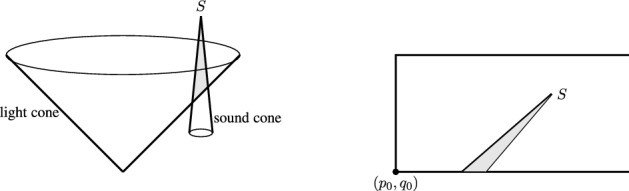
The grey shaded area in the infinite rectangular region $\mathcal{D}$ is a schematic depiction of the region bounded by the backward fluid characteristics emanating from a point $S\in \mathcal{D}$. The opening angle is of order $\sqrt{\epsilon }\ll 1$, which of course is precisely the speed of sound

Remark 9.2

It follows from (9.646)–(9.647) that

$$\begin{array}{c}\hfill \rho =\frac{1}{1-\epsilon }\frac{{(f^{+}{f}^{-})}^{\frac{1}{k_{+}-k_{-}}}}{r^{2+2\eta }}.\end{array}$$ 9.653

Moreover, from (2.82) and (9.646)–(9.647) we have $\frac{f^{+}}{f^{-}}=\frac{1}{{(1+\eta )}^2}{r}^{4\eta }{(u^q)}^4$, which leads to the relation

$$\begin{array}{c}\hfill \mathcal{U}=(1+\eta ){\mathrm{\Omega }}^2{(u^q)}^2={(1+\eta )}^2\frac{{\mathrm{\Omega }}^2}{r^{2\eta }}{\left(\frac{f^{+}}{f^{-}}\right)}^{\frac{1}{2}}.\end{array}$$ 9.654

Statement of the Local Well-Posedness Theorem

In order to flatten the the $g_{\text{RLP},\epsilon }$ metric at asymptotic infinity, we shall treat the system (2.83)–(2.84) and (9.648)–(9.649) as the evolutionary part and equations (2.86)–(2.85) as the constraints.

Fixing the Choice of Double-Null Coordinates

We now fix a choice of double-null coordinates which will then be used to dampen the tails of the solution and produce an asymptotically flat spacetimes containing a naked singularity. Let $({\tilde{\tau }}_0,R_0)\in {\tilde{\mathcal{D}}}_{\text{RLP},\epsilon }$ be a given point in the exterior region (see Definition 8.6 and (2.66) for the definition of ${\tilde{\mathcal{D}}}_{\text{RLP},\epsilon }$). Through $({\tilde{\tau }}_0,R_0)$ we consider the ingoing null-curve which intersects the outgoing null-curve ${\mathcal{B}}_1$ (given by $R=\frac{\sqrt{\epsilon }}{|Y^1|}\tilde{\tau }$) at some $(R_1,{\tilde{\tau }}_1)$ where by Lemma 8.8, $R_1>0$. We then fix the null-coordinate $p$ by demanding that

$$\begin{array}{c}\hfill p=-2(r-r_1)\text{along the ingoing null-geodesic through}(R_0,{\tilde{\tau }}_0),r_1:=\tilde{r}(R_1,{\tilde{\tau }}_1);\end{array}$$ 9.655

and demanding that the level sets of $p$ correspond to outgoing null-geodesics. The choice (9.655) normalises ${\mathcal{B}}_1$ to correspond to the hypersruface $\{p=0\}$ in the RLP-spacetime. Note that in the RLP spacetime, the ingoing curve through $({\tilde{\tau }}_0,R_0)$ terminates at the massive singularity $\mathcal{M}{\mathcal{S}}_{\epsilon }$ to the future.

Let now the outgoing null geodesic through $({\tilde{\tau }}_0,R_0)$ intersect the surface $\mathcal{N}$ (boundary of the past of the scaling origin $\mathcal{O}$) at $(R_{\ast },{\tilde{\tau }}_{\ast })$. We then fix the null coordinate $q$ by demanding that

$$\begin{array}{c}\hfill q=2(r-r_{\ast })\text{along the outgoing null-geodesic through}({\tilde{\tau }}_0,R_0),r_{\ast }:=\tilde{r}(R_{\ast },{\tilde{\tau }}_{\ast });\end{array}$$ 9.656

and demanding that the level sets of $q$ correspond to ingoing null-geodesics. The normalisation (9.656) makes the surface $\mathcal{N}$ correspond to the hypersurface $\{q=0\}$. A more detailed description of the RLP-spacetime in this double-null gauge is given in Lemma A.1.

Let $(p_0,q_0)$ be the point $({\tilde{\tau }}_0,R_0)$ in the above double-null gauge. We shall consider the seminfinite rectangular domain

$$\begin{array}{c}\hfill \mathcal{D}:=\{(p,q):p_0<p<0,q>q_0\},\end{array}$$ 9.657

where $|p_0|>0$ is sufficiently small, with data prescribed on the set $\underset{\_}{\mathcal{C}}\cup \mathcal{C},$ where

$$\begin{array}{cc}\hfill \underset{\_}{\mathcal{C}}& :=\left\{(p,q),,|,,q,=,q_0,,,,,p,\in ,[p_0,0]\right\},\hfill \end{array}$$ 9.658

$$\begin{array}{cc}\hfill \mathcal{C}& :=\left\{(p,q),,|,,p,=,p_0,,,,,q,\in ,[q_0,\infty )\right\}\hfill \end{array}$$ 9.659

correspond to the ingoing and the outgoing null-curves emanating from $(p_0,q_0)$ respectively. See Figure 6.

Norms and Local Well-Posedness

Fix $N_{\pm }>0$ so that

$$\begin{array}{c}\hfill N_{+}=N_{-}-4\eta ,N_{-}>\frac{k_{+}-k_{-}}{2}+2\eta \end{array}$$ 9.660

and let $0<\theta \ll 1$ be a small fixed constant. For any $f^{\pm }\in W^{2,\infty }(\overline{\mathcal{D}})$ and $(\mathrm{\Omega },\frac{r}{q})\in W^{3,\infty }(\overline{\mathcal{D}})$, we define the total norm by

$$\begin{array}{cc}\hfill \left|\left|\left|[,f^{\pm },,,\mathrm{\Omega },,,r,]\right|\right|\right|& :=\left|\left|\left|[,f^{\pm },]\right|\right|\right|+\left|\left|\left|[,\mathrm{\Omega },,,r,]\right|\right|\right|\hfill \end{array}$$ 9.661

where

$$\begin{array}{cc}\hfill \left|\left|\left|[,f^{\pm },]\right|\right|\right|& :=\Vert log(q^{N_{+}}{f}^{+}){\Vert }_{\infty }+\sum _{j=1}^2{\Vert q^j{\partial }_q^{j}log{f}^{+}\Vert }_{\infty }\hfill \end{array}$$ 9.662

$$\begin{array}{cc}& +\Vert log(q^{N_{-}}{f}^{-}){\Vert }_{\infty }+\sum _{j=1}^2{\Vert q^j{\partial }_q^{j}log{f}^{-}\Vert }_{\infty },\hfill \\ \hfill \left|\left|\left|[,\mathrm{\Omega },,,r,]\right|\right|\right|& ={\Vert log\mathrm{\Omega }\Vert }_{\infty }+\sum _{j=1}^3{\Vert q^{j+\theta }{\partial }_q^{j}log\mathrm{\Omega }\Vert }_{\infty }\hfill \end{array}$$ 9.663

$$\begin{array}{cc}& +\sum _{j=0}^3{\Vert q^{j-2}{\partial }_q^j(r^2)\Vert }_{\infty }+{∥\frac{q^2}{r^2}∥}_{\infty }+{∥\frac{q}{{\partial }_q(r^2)}∥}_{\infty },\hfill \end{array}$$ 9.664

and the data norm

$$\begin{array}{cc}\hfill \left|\left|\left|[f^{\pm },\mathrm{\Omega },r],{|}_{\underset{\_}{\mathcal{C}}\cup \mathcal{C}}\right|\right|\right|& :=\left|\left|\left|[f^{\pm }],{|}_{\underset{\_}{\mathcal{C}}\cup \mathcal{C}}\right|\right|\right|+\left|\left|\left|{[\mathrm{\Omega },r]|}_{\underset{\_}{\mathcal{C}}\cup \mathcal{C}}\right|\right|\right|\hfill \\ \hfill & :=\Vert log(q^{N_{+}}{f}^{+}){|}_{\underset{\_}{\mathcal{C}}\cup \mathcal{C}}{\Vert }_{\infty }+\sum _{j=1}^2\Vert q^j{\partial }_q^{j}log{f}^{+}{{|}_{\underset{\_}{\mathcal{C}}\cup \mathcal{C}}\Vert }_{\infty }\hfill \\ \hfill & +\Vert log(q^{N_{-}}{f}^{-}){|}_{\underset{\_}{\mathcal{C}}\cup \mathcal{C}}{\Vert }_{\infty }+\sum _{j=1}^2\Vert q^j{\partial }_q^{j}log{f}^{-}{{|}_{\underset{\_}{\mathcal{C}}\cup \mathcal{C}}\Vert }_{\infty }\hfill \\ \hfill & +{\Vert log\mathrm{\Omega }|}_{\underset{\_}{\mathcal{C}}\cup \mathcal{C}}{\Vert }_{\infty }+\sum _{j=1}^3\Vert q^{j+\theta }{\partial }_q^{j}log\mathrm{\Omega }{{|}_{\underset{\_}{\mathcal{C}}\cup \mathcal{C}}\Vert }_{\infty }\hfill \\ \hfill & +\sum _{j=0}^3\Vert q^{j-2}{\partial }_q^j(r^2){{|}_{\underset{\_}{\mathcal{C}}\cup \mathcal{C}}\Vert }_{\infty }+{∥\frac{q^2}{r^2},{|}_{\underset{\_}{\mathcal{C}}\cup \mathcal{C}}∥}_{\infty }+{∥\frac{q}{{\partial }_q(r^2)},{|}_{\underset{\_}{\mathcal{C}}\cup \mathcal{C}}∥}_{\infty }\hfill \\ \hfill & +\Vert q^{-1}{\partial }_p(r^2){{|}_{\underset{\_}{\mathcal{C}}}\Vert }_{\infty }+{∥\frac{r}{2},\left(1,+,\frac{4{\partial }_{p}r{\partial }_{q}r}{{\mathrm{\Omega }}^2}\right),{|}_{\underset{\_}{\mathcal{C}}}∥}_{\infty }\hfill \end{array}$$

We choose the data $({\widehat{f}}^{\pm },\widehat{r},\widehat{\mathrm{\Omega }})$ on $\underset{\_}{\mathcal{C}}$ to coincide with the corresponding data obtained by restricting the RLP-solution to $\underset{\_}{\mathcal{C}}$. Let $A_0>q_0$ be a real number to be specified later.

• (i)The data on $\mathcal{C}$ is chosen so that $[{\widehat{f}}^{\pm },\widehat{\mathrm{\Omega }},\widehat{r}]$ coincide with the exact selfsimilar $g_{\text{RLP},\epsilon }$ solution on the segment $\{(p,q)|p=p_0,q\in [q_0,A_0]\}$;
• (ii)${\widehat{f}}^{\pm }\in W^{2,\infty }(\mathcal{C}\cup \underset{\_}{\mathcal{C}})$, and $\widehat{\mathrm{\Omega }},\frac{\widehat{r}}{q}\in W^{3,\infty }(\underset{\_}{\mathcal{C}}\cup \mathcal{C})$ with $\left|\left|\left|[f^{\pm },\widehat{\mathrm{\Omega }},\widehat{r}],{|}_{\underset{\_}{\mathcal{C}}\cup \mathcal{C}}\right|\right|\right|<\infty$ and ${\widehat{f}}^{\pm },\widehat{\mathrm{\Omega }},\widehat{r}>0$;
• (iii)the constraint equations (2.85)–(2.86) hold on $\mathcal{C}$ and $\underset{\_}{\mathcal{C}}$ respectively.

Due to the choice of the double-null gauge (9.655)–(9.656), the metric coefficient $\widehat{r}$ is determined along $\mathcal{C}$. In order to impose the constraint (2.85) we can solve it for $\widehat{\mathrm{\Omega }}$. By (9.656) we have ${\partial }_{q}r=\frac{1}{2}$ and by (2.89) and Remark 9.2 we may rewrite (2.85) as

$$\begin{array}{c}\hfill \frac{1}{2}{\partial }_q({\mathrm{\Omega }}^{-2})=-\frac{\pi }{r}{(f^{+}{f}^{-})}^{\frac{1}{k_{+}-k_{-}}}{\left(\frac{f^{-}}{f^{+}}\right)}^{\frac{1}{2}}{\mathrm{\Omega }}^{-2}.\end{array}$$ 9.665

Moving the copy of ${\mathrm{\Omega }}^{-2}$ to the left-hand side and then integrating, we obtain the formula

$$\begin{array}{c}\hfill \mathrm{\Omega }(p_0,q)=\mathrm{\Omega }(p_0,q_0)exp\left({\int }_{q_0}^q,\frac{2\pi }{s+2r_{\ast }},{(f^{+}{f}^{-})}^{\frac{1}{k_{+}-k_{-}}},{\left(\frac{f^{-}}{f^{+}}\right)}^{\frac{1}{2}},,d,s\right).\end{array}$$ 9.666

Remark 9.3

(The Hawking mass) We recall the Hawking mass introduced in (2.10). It can be alternatively expressed via the formula

$$\begin{array}{c}\hfill m=\frac{r}{2}\left(1,+,\frac{4{\partial }_{p}r{\partial }_{q}r}{{\mathrm{\Omega }}^2}\right).\end{array}$$ 9.667

Using (2.83)–(2.86) one can show that for classical solutions of the Einstein-Euler system we have the identities

$$\begin{array}{cc}\hfill {\partial }_{p}m& =2\pi r^2{\mathrm{\Omega }}^2\left(T^{\mathit{pq}},{\partial }_p,r,-,T^{\mathit{qq}},{\partial }_q,r\right),\hfill \end{array}$$ 9.668

$$\begin{array}{cc}\hfill {\partial }_{q}m& =2\pi r^2{\mathrm{\Omega }}^2\left(T^{\mathit{pq}},{\partial }_q,r,-,T^{\mathit{pp}},{\partial }_p,r\right),\hfill \end{array}$$ 9.669

see for example Section 1.2 of [9]. Using (2.89) we may rewrite the right-hand side of (9.669) as $2\pi r^2(1-\epsilon )\rho \left({\partial }_q,r,-,(1+\eta ),{\mathrm{\Omega }}^2,{(u^p)}^2,{\partial }_p,r\right)$. Integration along a constant $p$-slice then gives

$$\begin{array}{c}\hfill m(p,q)=m(p,q_0)+2\pi (1-\epsilon ){\int }_{q_0}^q{r}^2\rho \left({\partial }_q,r,-,(1+\eta ),{\mathrm{\Omega }}^2,{(u^p)}^2,{\partial }_p,r\right)ds.\end{array}$$ 9.670

We now state the main local existence and uniqueness theorem for the characteristic problem described above.

Theorem 9.4

There exist sufficiently small ${\delta }_0>0$ such that for any $\delta \in (0,{\delta }_0)$ and $p_0=-\delta$, with initial boundary data satisfying (i)-(iii) above, there exists a unique asymptotically flat solution $[f^{\pm },\mathrm{\Omega },r]$ to the system (2.83)–(2.84) and (9.648)–(9.649), with $f^{\pm }\in W^{2,\infty }(\overline{\mathcal{D}})$ , $[\mathrm{\Omega },\frac{r}{q}]\in W^{3,\infty }(\overline{\mathcal{D}})$, and such that $\left|\left|\left|[,f^{\pm },,,\mathrm{\Omega },,,r,]\right|\right|\right|<\infty$. Moreover, this solution is a solution of the original system (2.83)–(2.88).

We shall prove Theorem 9.4 by the method of characteristics. Our strategy is to first solve the fluid evolution equations for $f^{\pm }$ given the effective fluid velocity $\mathcal{U}$ and the metric components $\mathrm{\Omega },r$. Then we will feed that back into the wave equations (2.83)–(2.84) for the metric components to obtain the bounds for $[r,\mathrm{\Omega }]$. To make this strategy work, in Section 9.3 we carefully look at the characteristics associated with the fluid evolution. After collecting some preparatory a priori bounds in Section 9.4, in Section 9.5 we use an iteration scheme to conclude the proof of Theorem 9.4.

Characteristics for the Fluid Evolution

Let ${\mathfrak{q}}_{\pm }(s)={\mathfrak{q}}_{\pm }(s;p,q)$ be the backward characteristics associated with the speeds $k_{\pm }\mathcal{U}$ such that

$$\begin{array}{cc}\hfill \frac{d{\mathfrak{q}}_{\pm }}{\mathit{ds}}(s;p,q)& =k_{\pm }\mathcal{U}(s,{\mathfrak{q}}_{\pm }(s;p,q)),s<p,\hfill \end{array}$$ 9.671

$$\begin{array}{cc}\hfill {\mathfrak{q}}_{\pm }(p;p,q)& =q.\hfill \end{array}$$ 9.672

Since our solutions as well as $\mathcal{U}$ reside in the domain $\mathcal{D}$ and the boundary, we track the backward characteristics $(s,{\mathfrak{q}}_{\pm }(s))$ until they leave the domain. In the next lemma, we show the existence and regularity properties of ${\mathfrak{q}}_{\pm }(s)$ and exit time $p_{\ast }=p_{\ast }(p,q)$ and position $q_{\ast }=q_{\ast }(p,q)$.

Lemma 9.5

Let $\ell \in \mathbb{N}$. Suppose $\mathcal{U}\in C^{\ell }(\overline{\mathcal{D}})$ or $W^{\ell ,\infty }(\overline{\mathcal{D}})$ and $\frac{1}{C_0}<\mathcal{U}<C_0$ on $\overline{\mathcal{D}}$ for some $C_0>1$. Then for any given $(p,q)\in \mathcal{D}$, there exist a unique exit time $p_{\ast }=p_{\ast }(p,q)$ and position $q_{\ast }=q_{\ast }(p,q)$ such that

1. A unique solution ${\mathfrak{q}}_{\pm }\in C^{\ell }((p_{\ast },p];C^{\ell }(\mathcal{D}))$ or $C^{\ell }((p_{\ast },p];W^{\ell ,\infty }(\mathcal{D}))$ of (9.671) and (9.672) exists so that $(s,{\mathfrak{q}}_{\pm }(s;p,q))\in \mathcal{D}$.

2. At $s=p_{\ast }$, $(p_{\ast },q_{\ast })\in \underset{\_}{\mathcal{C}}\cup \mathcal{C}$ where $q_{\ast }={\mathfrak{q}}_{\pm }(p_{\ast };p,q)$ and it satisfies

   $$\begin{array}{c}\hfill q-q_{\ast }={\int }_{p_{\ast }}^p{k}_{\pm }\mathcal{U}(s,{\mathfrak{q}}_{\pm }(s;p,q))ds.\end{array}$$ 9.673

   If $p_{\ast }>p_0$ then $q_{\ast }=q_0$.

3. $(p,q)\mapsto p_{\ast }(p,q)\in C(\mathcal{D})$.

4. If $p_{\ast }\ne p_0$, $p_{\ast }\in C^{\ell }(\mathcal{D})$ or $W^{\ell ,\infty }(\overline{\mathcal{D}})$.

In particular, if $q>q_0+k_{\pm }{C}_0(p-p_0)$, then $(p_{\ast },q_{\ast })=(p_0,q_{\ast })\in \mathcal{C}$.

Proof

We prove the claims for $\mathcal{U}\in C^{\ell }$ as the case of $\mathcal{U}\in W^{\ell ,\infty }$ follows in the same way. The local existence and uniqueness of ${\mathfrak{q}}_{\pm }\in C^{\ell }$ follows from $\mathcal{U}\in C^{\ell }$ via the Picard iteration

$$\begin{array}{c}\hfill {\mathfrak{q}}_{\pm }(s)=q-{\int }_s^p{k}_{\pm }\mathcal{U}(\tilde{s},{\mathfrak{q}}_{\pm }(\tilde{s};p,q))d\tilde{s}.\end{array}$$ 9.674

Thanks to the positive uniform bound of $\mathcal{U}$ and Grönwall, the solution can be continued as long as the characteristics belong to the domain $(s,{\mathfrak{q}}_{\pm }(s;p,q))\in \mathcal{D}$. Since $\mathcal{U}>\frac{1}{C_0}$, ${\mathfrak{q}}_{\pm }(s)<q-\frac{k_{\pm }}{C_0}(p-s)$, $(s,{\mathfrak{q}}_{\pm }(s))$ will exit the domain $\mathcal{D}$ either through the outgoing boundary $\mathcal{C}$ or through the ingoing boundary $\underset{\_}{\mathcal{C}}$. We denote such an exit time by $p_{\ast }$ and the associated value $q_{\ast }=q_{\pm }(p_{\ast };p,q)$ where $(p_{\ast },q_{\ast })\in \underset{\_}{\mathcal{C}}\cup \mathcal{C}$. Note that for each given $(p,q)\in \mathcal{D}$, $(p_{\ast },q_{\ast })$ is uniquely determined since the backward characteristics ${\mathfrak{q}}_{\pm }$ are unique. By integrating (9.671) from $s=p$ to $s=p_{\ast }$, we see that $(p_{\ast },q_{\ast })$ satisfies (9.673). We observe that if $(p_{\ast },q_{\ast })\in \underset{\_}{\mathcal{C}}$, $q_{\ast }=q_0$ and $p_0\le p_{\ast }<p$, and (9.673) reads as

$$\begin{array}{c}\hfill q-q_0={\int }_{p_{\ast }}^p{k}_{\pm }\mathcal{U}(s,{\mathfrak{q}}_{\pm }(s;p,q))ds.\end{array}$$ 9.675

If $(p_{\ast },q_{\ast })\in \mathcal{C}$, $p_{\ast }=p_0$ and $q_{\ast }$ is given by (9.673).

Clearly $p_{\ast }$ is continuous in $p$ and $q$. Since higher regularity of $p_{\ast }$ fails in general at the corner of the domain where $(p_{\ast },q_{\ast })=(p_0,q_0)$, we show the regularity when $p\ne p_0$. First let $(\tilde{p},\tilde{q})\in \mathcal{D}$ be given. Suppose ${\tilde{p}}_{\ast }=p_{\ast }(\tilde{p},\tilde{q})>p_0$. Consider a small neighborhood $\mathcal{B}$ of $(\tilde{p},\tilde{q})$ in $\mathcal{D}$ such that $I_1=p_{\ast }(\mathcal{B})$, $inf{I}_1>p_0$. Recalling (9.675), we define an auxiliary function $H:I_1\times \mathcal{B}\to \mathbb{R}$ by

$$\begin{array}{c}\hfill H({\overline{p}}_{\ast },p,q)=q-q_0-{\int }_{{\overline{p}}_{\ast }}^p{k}_{\pm }\mathcal{U}(s,{\mathfrak{q}}_{\pm }(s;p,q))ds.\end{array}$$

Then $H\in C^{\ell }$ since $\mathcal{U}\in C^{\ell }$, while we have $H({\tilde{p}}_{\ast },\tilde{p},\tilde{q})=0$ and ${\partial }_{{\overline{p}}_{\ast }}H({\tilde{p}}_{\ast },\tilde{p},\tilde{q})=k_{\pm }\mathcal{U}({\tilde{p}}_{\ast },{\tilde{q}}_{\ast })>0$. Therefore, by the implicit function theorem, $p_{\ast }=p_{\ast }(p,q)\in C^{\ell }$ in a small neighborhood of $(\tilde{p},\tilde{q})$.

Lastly, since $\mathcal{U}<C_0$, if $q>q_0+k_{\pm }{C}_0(p-p_0)$, the backward characteristics will intersect the outgoing surface $\mathcal{C}$, in which case $p_{\ast }=p_0$. $\square$

A Priori Bounds

In this subsection, we provide estimates for various quantities appearing the iteration scheme in terms of our norms. We will frequently use the following inequality: for any positive function $g>0$

$$\begin{array}{c}\hfill {max\{\Vert g\Vert }_{\infty },\Vert g^{-1}{\Vert }_{\infty }\}\le e^{{\Vert logg\Vert }_{\infty }}\end{array}$$ 9.676

which directly follows from $g=e^{logg}$ and $g^{-1}=e^{-logg}$.

Lemma 9.6

Suppose $\left|\left|\left|[,\mathrm{\Omega },,,r,]\right|\right|\right|<\infty$. Then the following holds:

$$\begin{array}{c}\hfill \sum _{j=0}^2{∥q^{j+1},{\partial }_q^j,\left(\frac{{\partial }_q\mathrm{\Omega }}{\mathrm{\Omega }},-,\eta ,\frac{{\partial }_{q}r}{r}\right)∥}_{\infty }\le M_1(\left|\left|\left|[,\mathrm{\Omega },,,r,]\right|\right|\right|),\end{array}$$ 9.677

$$\begin{array}{c}\hfill \sum _{j=1}^2{∥q^{j+3},{\partial }_q^j,\left(\frac{{\mathrm{\Omega }}^2}{r^3}\right)∥}_{\infty }\le M_2(\left|\left|\left|[,\mathrm{\Omega },,,r,]\right|\right|\right|),\end{array}$$ 9.678

where $M_1$ and $M_2$ are continuous functions of their arguments.

Proof

We start with (9.677). For $j=0$, it is easy to see that

$$\begin{array}{c}\hfill {∥q,\left(\frac{{\partial }_q\mathrm{\Omega }}{\mathrm{\Omega }},-,\eta ,\frac{{\partial }_{q}r}{r}\right)∥}_{\infty }\le \frac{1}{q_0^{\theta }}{\Vert q^{1+\theta }{\partial }_{q}log\mathrm{\Omega }\Vert }_{\infty }+\frac{\eta }{2}{∥\frac{q^2}{r^2}∥}_{\infty }{∥\frac{{\partial }_q(r^2)}{q}∥}_{\infty }\end{array}$$ 9.679

where the right-hand side is a continuous function of $\left|\left|\left|[,\mathrm{\Omega },,,r,]\right|\right|\right|$ by (9.676). For $j=1$, since

$${\partial }_q\left(\frac{{\partial }_q\mathrm{\Omega }}{\mathrm{\Omega }},-,\eta ,\frac{{\partial }_{q}r}{r}\right)={\partial }_q^{2}log\mathrm{\Omega }-\frac{\eta }{2}\frac{{\partial }_q^2(r^2)}{r^2}+\frac{\eta }{2}\frac{{({\partial }_q(r^2))}^2}{r^4}$$

we have

$$\begin{array}{cc}\hfill & {∥q^2,{\partial }_q,\left(\frac{{\partial }_q\mathrm{\Omega }}{\mathrm{\Omega }},-,\eta ,\frac{{\partial }_{q}r}{r}\right)∥}_{\infty }\le \frac{1}{q_0^{\theta }}{\Vert q^{2+\theta }{\partial }_q^{2}log\mathrm{\Omega }\Vert }_{\infty }\hfill \\ \hfill & +\frac{\eta }{2}{∥\frac{q^2}{r^2}∥}_{\infty }{\Vert {\partial }_q^2(r^2)\Vert }_{\infty }+\frac{\eta }{2}{∥\frac{q^2}{r^2}∥}_{\infty }^2{∥\frac{{\partial }_q(r^2)}{q}∥}_{\infty }^2\hfill \end{array}$$ 9.680

which shows (9.677). Lastly, from

$$\begin{array}{c}\hfill {\partial }_q^2\left(\frac{{\partial }_q\mathrm{\Omega }}{\mathrm{\Omega }},-,\eta ,\frac{{\partial }_{q}r}{r}\right)={\partial }_q^{3}log\mathrm{\Omega }-\frac{\eta }{2}\frac{{\partial }_q^3(r^2)}{r^2}+\frac{3\eta }{2}\frac{{\partial }_q(r^2){\partial }_q^2(r^2)}{r^4}-\eta \frac{{({\partial }_q(r^2))}^3}{r^6}\end{array}$$

we obtain

$$\begin{array}{c}\hfill \begin{array}{cc}\hfill {∥q^3,{\partial }_q^2,\left(\frac{{\partial }_q\mathrm{\Omega }}{\mathrm{\Omega }},-,\eta ,\frac{{\partial }_{q}r}{r}\right)∥}_{\infty }& \le \frac{1}{q_0^{\theta }}\Vert q^{3+\theta }{\partial }_q^3{log\mathrm{\Omega }\Vert }_{\infty }+\frac{\eta }{2}{∥\frac{q^2}{r^2}∥}_{\infty }{\Vert q{\partial }_q^3(r^2)\Vert }_{\infty }\hfill \\ \hfill & +\frac{3\eta }{2}{∥\frac{q^2}{r^2}∥}_{\infty }^2{∥\frac{{\partial }_q(r^2)}{q}∥}_{\infty }^2{\Vert {\partial }_q^2(r^2)\Vert }_{\infty }+\frac{\eta }{2}{∥\frac{q^2}{r^2}∥}_{\infty }^3{∥\frac{{\partial }_q(r^2)}{q}∥}_{\infty }^3.\hfill \end{array}\end{array}$$ 9.681

This completes the proof of (9.677). The estimation of (9.678) follows similarly, we omit the details. $\square$

Lemma 9.7

($\mathcal{U}$ bounds) Suppose $\left|\left|\left|[,f^{\pm },,,\mathrm{\Omega },,,r,]\right|\right|\right|<\infty$. Then the following holds:

$$\begin{array}{c}\hfill {\Vert \mathcal{U}\Vert }_{\infty }+\Vert {\mathcal{U}}^{-1}{\Vert }_{\infty }+\sum _{j=1}^2{\Vert q^j{\partial }_q^j\mathcal{U}\Vert }_{\infty }\le M_3(\left|\left|\left|[,f^{\pm },,,\mathrm{\Omega },,,r,]\right|\right|\right|)\end{array}$$ 9.682

where $M_3$ is a continuous function of its argument.

Proof

From the first condition of our choice $N_{\pm }$ in (9.660), we may rewrite $\mathcal{U}$ as

$$\begin{array}{c}\hfill \mathcal{U}={(1+\eta )}^2{\mathrm{\Omega }}^2{\left(\frac{q}{r}\right)}^{2\eta }{\left(\frac{q^{N_{+}}{f}^{+}}{q^{N_{-}}{f}^{-}}\right)}^{\frac{1}{2}}.\end{array}$$

Then by (9.676), we see that

$$\begin{array}{c}\hfill \Vert {\mathcal{U}}^{\pm 1}{\Vert }_{\infty }\le {(1+\eta )}^{\pm 2}{∥\frac{q^2}{r^2}∥}_{\infty }^{\pm \eta }{e}^{{2\Vert log\mathrm{\Omega }\Vert }_{\infty }+\frac{1}{2}\Vert log(q^{N_{+}}{f}^{+}){\Vert }_{\infty }+\frac{1}{2}{\Vert log(q^{N_{-}}{f}^{-})\Vert }_{\infty }}\end{array}$$ 9.683

which shows (9.682) for ${\Vert \mathcal{U}\Vert }_{\infty }+{\Vert {\mathcal{U}}^{-1}\Vert }_{\infty }$. Next computing ${\partial }_q\mathcal{U}$ as

$$\begin{array}{c}\hfill {\partial }_q\mathcal{U}=\left(2,\left(\frac{{\partial }_q\mathrm{\Omega }}{\mathrm{\Omega }},-,\eta ,\frac{{\partial }_{q}r}{r}\right),+,\frac{1}{2},{\partial }_q,log,f^{+},-,\frac{1}{2},{\partial }_q,log,f^{-}\right)\mathcal{U}\end{array}$$ 9.684

we obtain

$$\begin{array}{c}\hfill \Vert q{\partial }_q{\mathcal{U}\Vert }_{\infty }\le \left(2,{∥q,\left(\frac{{\partial }_q\mathrm{\Omega }}{\mathrm{\Omega }},-,\eta ,\frac{{\partial }_{q}r}{r}\right)∥}_{\infty },+,\frac{1}{2},\Vert q,{\partial }_q,log,f^{+},{\Vert }_{\infty },+,\frac{1}{2},{\Vert q{\partial }_{q}log{f}^{-}\Vert }_{\infty }\right){\Vert \mathcal{U}\Vert }_{\infty }.\end{array}$$ 9.685

Together with (9.679), it implies (9.682) for $j=1$. Moreover, since

$$\begin{array}{c}\hfill {\partial }_q^2\mathcal{U}=\left(2,{\partial }_q,\left(\frac{{\partial }_q\mathrm{\Omega }}{\mathrm{\Omega }},-,\eta ,\frac{{\partial }_{q}r}{r}\right),+,\frac{1}{2},{\partial }_q^2,log,f^{+},-,\frac{1}{2},{\partial }_q^2,log,f^{-}\right)\mathcal{U}+\frac{{({\partial }_q\mathcal{U})}^2}{\mathcal{U}}\end{array}$$ 9.686

we have

$$\begin{array}{c}\hfill \begin{array}{cc}\hfill \Vert q^2{\partial }_q^2{\mathcal{U}\Vert }_{\infty }& \le (2{∥q^2,{\partial }_q,\left(\frac{{\partial }_q\mathrm{\Omega }}{\mathrm{\Omega }},-,\eta ,\frac{{\partial }_{q}r}{r}\right)∥}_{\infty }+\frac{1}{2}\Vert q^2{\partial }_q^{2}log{f}^{+}{\Vert }_{\infty }+\frac{1}{2}\Vert q^2{\partial }_q^{2}log{f}^{-}{\Vert }_{\infty }){\Vert \mathcal{U}\Vert }_{\infty }\hfill \\ \hfill & +\Vert {\mathcal{U}}^{-1}{\Vert }_{\infty }{\Vert q{\partial }_q\mathcal{U}\Vert }_{\infty }^2.\hfill \end{array}\end{array}$$ 9.687

Using (9.680) and (9.685), we deduce (9.682), where we recall (9.661). $\square$

Remark 9.8

The relation $N_{+}=N_{-}-4\eta$ in (9.660) is importantly used to ensure the boundedness (both upper and lower) of the transport speed $\mathcal{U}$.

We introduce the constant $\beta >0$:

$$\begin{array}{c}\hfill \beta :=2\eta +\frac{N_{+}+N_{-}}{k_{+}-k_{-}}-1=2\eta +\frac{2N_{-}-(k_{+}-k_{-}+4\eta )}{k_{+}-k_{-}}>0,\end{array}$$ 9.688

where we have used (9.660) in the second equality.

Lemma 9.9

Suppose $\left|\left|\left|[,f^{\pm },,,\mathrm{\Omega },,,r,]\right|\right|\right|<\infty$. Then the following bounds hold:

$$\begin{array}{c}\hfill \sum _{j=0}^2{∥q^{j+1+\beta },{\partial }_q^j,\left(\frac{{\mathrm{\Omega }}^2}{r^{2\eta }},{(f^{+}{f}^{-})}^{\frac{1}{k_{+}-k_{-}}}\right)∥}_{\infty }\le M_4(\left|\left|\left|[,f^{\pm },,,\mathrm{\Omega },,,r,]\right|\right|\right|),\end{array}$$ 9.689

$$\begin{array}{c}\hfill \sum _{j=0}^2{∥q^{j+3+\beta },{\partial }_q^j,\left(\frac{{\mathrm{\Omega }}^2}{r^{2+2\eta }},{(f^{+}{f}^{-})}^{\frac{1}{k_{+}-k_{-}}}\right)∥}_{\infty }\le M_5(\left|\left|\left|[,f^{\pm },,,\mathrm{\Omega },,,r,]\right|\right|\right|),\end{array}$$ 9.690

where $M_4$ and $M_5$ are continuous functions of their arguments.

Proof

We will first prove (9.689). We start with $j=0$. Using (9.688), we rewrite $\mathfrak{H}:=\frac{{\mathrm{\Omega }}^2}{r^{2\eta }}{(f^{+}{f}^{-})}^{\frac{1}{k_{+}-k_{-}}}$ as

$$\begin{array}{c}\hfill q^{1+\beta }\mathfrak{H}=q^{1+\beta }\frac{{\mathrm{\Omega }}^2}{r^{2\eta }}{(f^{+}{f}^{-})}^{\frac{1}{k_{+}-k_{-}}}={\mathrm{\Omega }}^2{\left(\frac{q}{r}\right)}^{2\eta }{\left(q^{N_{+}},f^{+},q^{N_{-}},f^{-}\right)}^{\frac{1}{k_{+}-k_{-}}}\end{array}$$

from which we have

$$\begin{array}{c}\hfill {∥q^{1+\beta },\mathfrak{H}∥}_{\infty }\le {\Vert \mathrm{\Omega }\Vert }_{\infty }^2{∥\frac{q^2}{r^2}∥}_{\infty }^{\eta }(\Vert q^{N_{+}}{f}^{+}{\Vert }_{\infty }\Vert q^{N_{-}}{f}^{-}{{\Vert }_{\infty })}^{\frac{1}{k_{+}-k_{-}}}.\end{array}$$ 9.691

By (9.676), the claim immediately follows. We next compute

$$\begin{array}{c}\hfill {\partial }_q\mathfrak{H}=\left(2,\left(\frac{{\partial }_q\mathrm{\Omega }}{\mathrm{\Omega }},-,\eta ,\frac{{\partial }_{q}r}{r}\right),+,\frac{{\partial }_{q}log{f}^{+}+{\partial }_{q}log{f}^{-}}{k_{+}-k_{-}}\right)\mathfrak{H}\end{array}$$ 9.692

and obtain

$$\begin{array}{c}\hfill \Vert q^{2+\beta }{\partial }_q{\mathfrak{H}\Vert }_{\infty }\le \left(2,{∥q,\left(\frac{{\partial }_q\mathrm{\Omega }}{\mathrm{\Omega }},-,\eta ,\frac{{\partial }_{q}r}{r}\right)∥}_{\infty },+,\frac{\Vert q{\partial }_{q}log{f}^{+}{\Vert }_{\infty }+{\Vert q{\partial }_{q}log{f}^{-}\Vert }_{\infty }}{k_{+}-k_{-}}\right){\Vert q^{1+\beta }\mathfrak{H}\Vert }_{\infty }.\end{array}$$ 9.693

With (9.679) and (9.691), it gives (9.689) for $j=1$. We next have

$$\begin{array}{c}\hfill \begin{array}{cc}\hfill {\partial }_q^2\mathfrak{H}& =\left(2,{\partial }_q,\left(\frac{{\partial }_q\mathrm{\Omega }}{\mathrm{\Omega }},-,\eta ,\frac{{\partial }_{q}r}{r}\right),+,\frac{{\partial }_q^{2}log{f}^{+}+{\partial }_q^{2}log{f}^{-}}{k_{+}-k_{-}}\right)\mathfrak{H}\hfill \\ \hfill & +\left(2,\left(\frac{{\partial }_q\mathrm{\Omega }}{\mathrm{\Omega }},-,\eta ,\frac{{\partial }_{q}r}{r}\right),+,\frac{{\partial }_{q}log{f}^{+}+{\partial }_{q}log{f}^{-}}{k_{+}-k_{-}}\right){\partial }_q\mathfrak{H},\hfill \end{array}\end{array}$$ 9.694

and therefore

$$\begin{array}{c}\hfill \begin{array}{cc}\hfill \Vert q^{3+\beta }{\partial }_q^2{\mathfrak{H}\Vert }_{\infty }& \le (2{∥q^2,{\partial }_q,\left(\frac{{\partial }_q\mathrm{\Omega }}{\mathrm{\Omega }},-,\eta ,\frac{{\partial }_{q}r}{r}\right)∥}_{\infty }+\frac{\Vert q^2{\partial }_q^{2}log{f}^{+}{\Vert }_{\infty }+{\Vert q^2{\partial }_q^{2}log{f}^{-}\Vert }_{\infty }}{k_{+}-k_{-}}){\Vert q^{1+\beta }\mathfrak{H}\Vert }_{\infty }\hfill \\ \hfill & +\left(2,{∥q,\left(\frac{{\partial }_q\mathrm{\Omega }}{\mathrm{\Omega }},-,\eta ,\frac{{\partial }_{q}r}{r}\right)∥}_{\infty },+,\frac{\Vert q{\partial }_{q}log{f}^{+}{\Vert }_{\infty }+{\Vert q{\partial }_{q}log{f}^{-}\Vert }_{\infty }}{k_{+}-k_{-}}\right){\Vert q^{2+\beta }{\partial }_q\mathfrak{H}\Vert }_{\infty }.\hfill \end{array}\end{array}$$ 9.695

Hence the claim follows from (9.691), (9.693) and (9.677).

The proof of (9.690) follows easily from (9.689) by applying the product rule for $\frac{{\mathrm{\Omega }}^2}{r^{2+2\eta }}{(f^{+}{f}^{-})}^{\frac{1}{k_{+}-k_{-}}}=r^{-2}\mathfrak{H}$ or by estimating them directly in the same way as done for (9.689). We omit the details. $\square$

In the iteration scheme, we will make use of the Hawking mass m given in (9.667). From (9.669) and (2.82) we see that the Hawking mass satisfies

$$\begin{array}{c}\hfill \begin{array}{cc}\hfill {\partial }_{q}m& =2\pi r^2\left[(1-\epsilon ),\rho ,{\partial }_q,r,-,(1+\epsilon ),{\mathrm{\Omega }}^{-2},\rho ,{(u^q)}^{-2},{\partial }_p,r\right]\hfill \\ \hfill & =2\pi {(f^{+}{f}^{-})}^{\frac{1}{k_{+}-k_{-}}}\left[\frac{1}{r^{2\eta }},{\partial }_q,r,-,{\mathrm{\Omega }}^{-2},{\left(\frac{f^{-}}{f^{+}}\right)}^{\frac{1}{2}},{\partial }_p,r\right].\hfill \end{array}\end{array}$$ 9.696

We observe that p-derivatives are not featured in our function space hierarchy, however ${\partial }_{p}r$ appears in the above expression. To go around this difficulty, we observe that (2.83) can be formally rewritten in the form

$$\begin{array}{c}\hfill {\partial }_{\mathit{pq}}(r^2)=-\frac{{\mathrm{\Omega }}^2}{2}+2\pi r^2{\mathrm{\Omega }}^4{T}^{\mathit{pq}}=-\frac{{\mathrm{\Omega }}^2}{2}+\frac{2\pi {\mathrm{\Omega }}^2}{r^{2\eta }}{(f^{+}{f}^{-})}^{\frac{1}{k_{+}-k_{-}}},\end{array}$$ 9.697

where we have used (2.89) and (9.653) in the second equality. Therefore, rather than directly estimating m from (9.667), we slightly abuse notation, and redefine m to be

$$\begin{array}{c}\hfill m(p,q):=m(p,q_0)+{\int }_{q_0}^q\left(2,\pi ,{(f^{+}{f}^{-})}^{\frac{1}{k_{+}-k_{-}}},\left[\frac{1}{r^{2\eta }},{\partial }_q,r,-,\frac{{\mathrm{\Omega }}^{-2}}{2r},{\left(\frac{f^{-}}{f^{+}}\right)}^{\frac{1}{2}},\mathfrak{s}\right]\right)d\tilde{q}\end{array}$$ 9.698

where

$$\begin{array}{cc}\hfill m(p,q_0)& :=\frac{\widehat{r}}{2}\left(1,+,\frac{4{\partial }_p\widehat{r}{\partial }_q\widehat{r}}{{\widehat{\mathrm{\Omega }}}^2}\right){|}_{(p,q_0)},\hfill \end{array}$$ 9.699

$$\begin{array}{cc}\hfill \mathfrak{s}(p,q)& :={\partial }_p({\widehat{r}}^2){|}_{(p,q_0)}+{\int }_{q_0}^q\left[-,\frac{{\mathrm{\Omega }}^2}{2},+,\frac{2\pi {\mathrm{\Omega }}^2}{r^{2\eta }},{(f^{+}{f}^{-})}^{\frac{1}{k_{+}-k_{-}}}\right]d\tilde{q}.\hfill \end{array}$$ 9.700

We observe that ${\partial }_p\widehat{r}$ is well-defined at $(p,q_0)$ since the data there is given by the exact selfsimilar RLP-solution. We note that $\mathfrak{s}$ corresponds exactly to ${\partial }_p(r^2)$ for a $C^2$-solution of the problem. In the following, we show that m in (9.698) can be estimated by using the norm $\left|\left|\left|[,f^{\pm },,,\mathrm{\Omega },,,r,]\right|\right|\right|$.

Lemma 9.10

Suppose $\left|\left|\left|[,f^{\pm },,,\mathrm{\Omega },,,r,]\right|\right|\right|<\infty$. Then the following holds:

$$\begin{array}{cc}\hfill {\Vert m\Vert }_{\infty }& \le \left|\left|\left|{[\mathrm{\Omega },r]|}_{\underset{\_}{\mathcal{C}}\cup \mathcal{C}}\right|\right|\right|+M_6(\left|\left|\left|[,f^{\pm },,,\mathrm{\Omega },,,r,]\right|\right|\right|),\hfill \end{array}$$ 9.701

$$\begin{array}{cc}\hfill \sum _{j=1}^2{\Vert q^{j+\beta }{\partial }_q^{j}m\Vert }_{\infty }& \le M_7(\left|\left|\left|[,f^{\pm },,,\mathrm{\Omega },,,r,]\right|\right|\right|),\hfill \end{array}$$ 9.702

where $M_6$ and $M_7$ are continuous functions of its argument.

Proof

We first observe that from (9.700) using $q>q_0$ and $\frac{q-q_0}{q}<1$

$$\begin{array}{c}\hfill \Vert q^{-1}{\mathfrak{s}\Vert }_{\infty }\le {∥\frac{{\partial }_p({\widehat{r}}^2)}{q},{|}_{(p,q_0)}∥}_{\infty }+\frac{{\Vert \mathrm{\Omega }\Vert }_{\infty }^2}{2}+\frac{2\pi }{q_0^{1+\beta }}{∥q^{1+\beta },\frac{{\mathrm{\Omega }}^2}{r^{2\eta }},{(f^{+}{f}^{-})}^{\frac{1}{k_{+}-k_{-}}}∥}_{\infty }\end{array}$$ 9.703

and

$$\begin{array}{c}\hfill \Vert {\partial }_q{\mathfrak{s}\Vert }_{\infty }\le \frac{{\Vert \mathrm{\Omega }\Vert }_{\infty }^2}{2}+\frac{2\pi }{q_0^{1+\beta }}{∥q^{1+\beta },\frac{{\mathrm{\Omega }}^2}{r^{2\eta }},{(f^{+}{f}^{-})}^{\frac{1}{k_{+}-k_{-}}}∥}_{\infty }\end{array}$$ 9.704

From the definition of the boundary data norm, we have $|m(p,q_0)|\le \left|\left|\left|{[\mathrm{\Omega },r]|}_{\underset{\_}{\mathcal{C}}\cup \mathcal{C}}\right|\right|\right|$. For the integral term in (9.698), using (9.688) and (9.660), we rewrite the integrand as

$$\begin{array}{c}\hfill \begin{array}{c}\hfill q^{-1-\beta }{(q^{N_{+}}{f}^{+}{q}^{N_{-}}{f}^{-})}^{\frac{1}{k_{+}-k_{-}}}\left[\frac{q^{2\eta }}{r^{2\eta }},{\partial }_q,r,-,{\mathrm{\Omega }}^{-2},\frac{q}{2r},{\left(\frac{q^{N_{-}}{f}^{-}}{q^{N_{+}}{f}^{+}}\right)}^{\frac{1}{2}},\frac{\mathfrak{s}}{q}\right]\end{array}\end{array}$$ 9.705

so that

$$\begin{array}{c}\hfill \begin{array}{cc}& \left|{\int }_{q_0}^q,\left(2,\pi ,{(f^{+}{f}^{-})}^{\frac{1}{k_{+}-k_{-}}},\left[\frac{1}{r^{2\eta }},{\partial }_q,r,-,\frac{{\mathrm{\Omega }}^{-2}}{2r},{\left(\frac{f^{-}}{f^{+}}\right)}^{\frac{1}{2}},\mathfrak{s}\right]\right),d,\tilde{q}\right|\hfill \\ \hfill & \le \frac{1}{\beta q_0^{\beta }}(\Vert q^{N_{+}}{f}^{+}{\Vert }_{\infty }\Vert q^{N_{-}}{f}^{-}{{\Vert }_{\infty })}^{\frac{1}{k_{+}-k_{-}}}\hfill \\ \hfill & ·\left[\frac{1}{2},\Vert ,\frac{q}{r},{\Vert }_{\infty }^{2\eta +1},\Vert ,q^{-1},{\partial }_q,(r^2),{\Vert }_{\infty },+,\frac{1}{2},\Vert ,{\mathrm{\Omega }}^{-1},{\Vert }_{\infty }^2,\Vert ,\frac{q}{r},{\Vert }_{\infty },\Vert ,q^{N_{-}},f^{-},{\Vert }_{\infty }^{\frac{1}{2}},\Vert ,{(q^{N_{+}}{f}^{+})}^{-1},{\Vert }_{\infty }^{\frac{1}{2}},{\Vert q^{-1}\mathfrak{s}\Vert }_{\infty }\right]\hfill \end{array}\end{array}$$

where we have used ${\int }_{q_0}^q{\tilde{q}}^{-1-\beta }d\tilde{q}\le \frac{1}{\beta q_0^{\beta }}$. Hence, using (9.676), we deduce (9.701). Moreover since

$$\begin{array}{c}\hfill {\partial }_{q}m=2\pi {(f^{+}{f}^{-})}^{\frac{1}{k_{+}-k_{-}}}\left[\frac{1}{r^{2\eta }},{\partial }_q,r,-,\frac{{\mathrm{\Omega }}^{-2}}{2r},{\left(\frac{f^{-}}{f^{+}}\right)}^{\frac{1}{2}},\mathfrak{s}\right]\end{array}$$ 9.706

from (9.705), we immediately obtain

$$\begin{array}{c}\hfill \begin{array}{cc}\hfill \Vert q^{1+\beta }{\partial }_q{m\Vert }_{\infty }& \le 2\pi (\Vert q^{N_{+}}{f}^{+}{\Vert }_{\infty }\Vert q^{N_{-}}{f}^{-}{{\Vert }_{\infty })}^{\frac{1}{k_{+}-k_{-}}}\hfill \\ \hfill & ·\left[\frac{1}{2},\Vert ,\frac{q}{r},{\Vert }_{\infty }^{2\eta +1},\Vert ,q^{-1},{\partial }_q,(r^2),{\Vert }_{\infty },+,\frac{1}{2},\Vert ,{\mathrm{\Omega }}^{-1},{\Vert }_{\infty }^2,\Vert ,\frac{q}{r},{\Vert }_{\infty },\Vert ,q^{N_{-}},f^{-},{\Vert }_{\infty }^{\frac{1}{2}},\Vert ,{(q^{N_{+}}{f}^{+})}^{-1},{\Vert }_{\infty }^{\frac{1}{2}},{\Vert q^{-1}\mathfrak{s}\Vert }_{\infty }\right]\hfill \end{array}\end{array}$$ 9.707

which shows (9.702) for $j=1$. Lastly, we compute ${\partial }_q^{2}m$ as

$$\begin{array}{c}\hfill \begin{array}{cc}& {\partial }_q^{2}m=\pi {(f^{+}{f}^{-})}^{\frac{1}{k_{+}-k_{-}}}\left[\frac{1}{r^{2\eta +1}},{\partial }_q^2,(r^2),-,\frac{{\mathrm{\Omega }}^{-2}}{r},{\left(\frac{f^{-}}{f^{+}}\right)}^{\frac{1}{2}},{\partial }_q,\mathfrak{s}\right]\hfill \\ \hfill & +\pi \frac{{(f^{+}{f}^{-})}^{\frac{1}{k_{+}-k_{-}}}}{r^{2\eta }}\frac{{\partial }_q(r^2)}{r}\left(\frac{{\partial }_{q}log{f}^{+}+{\partial }_{q}log{f}^{-}}{k_{+}-k_{-}},-,\frac{2\eta +1}{2},\frac{{\partial }_q(r^2)}{r^2}\right)\hfill \\ \hfill & -\pi {\mathrm{\Omega }}^{-2}{(f^{+}{f}^{-})}^{\frac{1}{k_{+}-k_{-}}}{\left(\frac{f^{-}}{f^{+}}\right)}^{\frac{1}{2}}\frac{\mathfrak{s}}{r}\left(-,2,{\partial }_q,log,\mathrm{\Omega },+,c_1,{\partial }_q,log,f^{+},+,c_2,{\partial }_q,log,f^{+},-,\frac{1}{2},\frac{{\partial }_q(r^2)}{r^2}\right)\hfill \end{array}\end{array}$$ 9.708

where $c_1=\frac{1}{k_{+}-k_{-}}-\frac{1}{2}$ and $c_2=\frac{1}{k_{+}-k_{-}}+\frac{1}{2}$. Following the same strategy, it is now clear that $\Vert q^{2+\beta }{\partial }_q^2{m\Vert }_{\infty }$ is bounded by a continuous function of $\left|\left|\left|[,f^{\pm },,,\mathrm{\Omega },,,r,]\right|\right|\right|$. This finishes the proof. $\square$

Proof of the Local Well-Posedness

Iteration Scheme

We now set up the iteration scheme. Let $[f_n^{\pm },{\mathrm{\Omega }}_n,r_n]$ be given so that $\left|\left|\left|[,f_n^{\pm },,,{\mathrm{\Omega }}_n,,,r_n,]\right|\right|\right|<\infty$. And let ${\mathcal{U}}_n$ and $m_n$ be given in (9.654) and (9.698) where $[f,\mathrm{\Omega },r]=[f_n^{\pm },{\mathrm{\Omega }}_n,r_n]$:

$$\begin{array}{c}\hfill {\mathcal{U}}_n={(1+\eta )}^2\frac{{({\mathrm{\Omega }}_n)}^2}{{(r_n)}^{2\eta }}{\left(\frac{f_n^{+}}{f_n^{-}}\right)}^{\frac{1}{2}}\end{array}$$

and

$$\begin{array}{c}\hfill m_n=m(p,q_0)+{\int }_{q_0}^q\left(2,\pi ,{(f_n^{+}{f}_n^{-})}^{\frac{1}{k_{+}-k_{-}}},\left[\frac{1}{{(r_n)}^{2\eta }},{\partial }_q,r_n,-,\frac{1}{2},\frac{{({\mathrm{\Omega }}_n)}^{-2}}{(r_n)},{\left(\frac{f_n^{-}}{f_n^{+}}\right)}^{\frac{1}{2}},{\mathfrak{s}}_n\right]\right)d\tilde{q}.\end{array}$$

Here ${\mathfrak{s}}_n$ is given by the right-hand side of (9.700) where $[f^{\pm },\mathrm{\Omega },r]=[f_n^{\pm },{\mathrm{\Omega }}_n,r_n]$. We then define $[f_{n+1}^{\pm },{\mathrm{\Omega }}_{n+1},r_{n+1}]$ to be the solution of the following system

$$\begin{array}{cc}& {\partial }_p{f}_{n+1}^{\pm }+k_{\pm }{\mathcal{U}}_n{\partial }_q{f}_{n+1}^{\pm }\pm 2k_{\pm }(2\frac{{\partial }_q{\mathrm{\Omega }}_n}{{\mathrm{\Omega }}_n}-2\eta \frac{{\partial }_q{r}_n}{r_n}){\mathcal{U}}_n{f}_{n+1}^{\pm }=0,\hfill \end{array}$$ 9.709

$$\begin{array}{cc}& {\partial }_p{\partial }_q[{(r_{n+1})}^2]=-\frac{{({\mathrm{\Omega }}_n)}^2}{2}+2\pi \frac{{({\mathrm{\Omega }}_n)}^2}{{(r_n)}^{2\eta }}{(f_n^{+}{f}_n^{-})}^{\frac{1}{k_{+}-k_{-}}},\hfill \end{array}$$ 9.710

$$\begin{array}{cc}& {\partial }_p{\partial }_{q}log{\mathrm{\Omega }}_{n+1}=\frac{{({\mathrm{\Omega }}_n)}^2}{2{(r_n)}^2}\frac{m_n}{r_n}-(1+\eta )\pi \frac{{({\mathrm{\Omega }}_n)}^2}{{(r_n)}^{2+2\eta }}{(f_n^{+}{f}_n^{-})}^{\frac{1}{k_{+}-k_{-}}},\hfill \end{array}$$ 9.711

with given characteristic data $[f_{n+1}^{\pm },{\mathrm{\Omega }}_{n+1},r_{n+1}]=[{\widehat{f}}^{\pm },\widehat{\mathrm{\Omega }},\widehat{r}]{|}_{\underset{\_}{\mathcal{C}}\cup \mathcal{C}}$ satisfying the conditions (i)–(iii) as in Theorem 9.4. We note that for exact solutions, (9.710)-(9.711) are equivalent to (2.83), (2.84).

Our next goal is to prove the solvability of the iterative system (9.709)-(9.711) and derive the uniform bounds of $\left|\left|\left|[,f_{n+1}^{\pm },,,{\mathrm{\Omega }}_{n+1},,,r_{n+1},]\right|\right|\right|$ for sufficiently small $\delta >0$. Let $A:=max\{4,1+\frac{1}{\theta q_0^{\theta }}\}$.

Proposition 9.11

Let the characteristic data $[{\widehat{f}}^{\pm },\widehat{\mathrm{\Omega }},\widehat{r}]$ satisfying the assumptions of Theorem 9.4 be given. Suppose $\left|\left|\left|[,f_n^{\pm },,,{\mathrm{\Omega }}_n,,,r_n,]\right|\right|\right|\le 2A\left|\left|\left|[{\widehat{f}}^{\pm },\widehat{\mathrm{\Omega }},\widehat{r}],{|}_{\underset{\_}{\mathcal{C}}\cup \mathcal{C}}\right|\right|\right|$. Then there exist sufficiently small ${\delta }_0>0$ depending only on $\left|\left|\left|[{\widehat{f}}^{\pm },\widehat{\mathrm{\Omega }},\widehat{r}],{|}_{\underset{\_}{\mathcal{C}}\cup \mathcal{C}}\right|\right|\right|$ such that for all $\delta \in (0,{\delta }_0)$ there exists a unique solution $f_{n+1}^{\pm }\in W^{2,\infty }(\overline{\mathcal{D}})$, $[{\mathrm{\Omega }}_{n+1},\frac{r_{n+1}}{q}]\in W^{3,\infty }(\overline{\mathcal{D}})$ to (9.709)-(9.711) with $[f_{n+1}^{\pm },{\mathrm{\Omega }}_{n+1},r_{n+1}]=[{\widehat{f}}^{\pm },\widehat{\mathrm{\Omega }},\widehat{r}]$ on $\underset{\_}{\mathcal{C}}\cup \mathcal{C}$ satisfying

$$\begin{array}{c}\hfill \left|\left|\left|[,f_{n+1}^{\pm },,,{\mathrm{\Omega }}_{n+1},,,r_{n+1},]\right|\right|\right|\le 2A\left|\left|\left|[{\widehat{f}}^{\pm },\widehat{\mathrm{\Omega }},\widehat{r}],{|}_{\underset{\_}{\mathcal{C}}\cup \mathcal{C}}\right|\right|\right|.\end{array}$$ 9.712

Proposition 9.11 immediately follows from the following two lemmas.

Lemma 9.12

(Solving the Euler part) Assume the same as in Proposition 9.11. Then there exist sufficiently small ${\delta }_0>0$ depending only on $\left|\left|\left|[{\widehat{f}}^{\pm },\widehat{\mathrm{\Omega }},\widehat{r}],{|}_{\underset{\_}{\mathcal{C}}\cup \mathcal{C}}\right|\right|\right|$ such that for all $\delta \in (0,{\delta }_0)$ there exists a unique solution $f_{n+1}^{\pm }\in W^{2,\infty }(\overline{\mathcal{D}})$ to (9.709) with $f_{n+1}^{\pm }={\widehat{f}}^{\pm }$ on $\underset{\_}{\mathcal{C}}\cup \mathcal{C}$ satisfying

$$\begin{array}{c}\hfill \left|\left|\left|[,f_{n+1}^{\pm },]\right|\right|\right|\le 2\left|\left|\left|[{\widehat{f}}^{\pm }],{|}_{\underset{\_}{\mathcal{C}}\cup \mathcal{C}}\right|\right|\right|+A\left|\left|\left|[{\widehat{f}}^{\pm },\widehat{\mathrm{\Omega }},\widehat{r}],{|}_{\underset{\_}{\mathcal{C}}\cup \mathcal{C}}\right|\right|\right|.\end{array}$$ 9.713

Lemma 9.13

(Solving the metric part) Assume the same as in Proposition 9.11. Then there exist sufficiently small ${\delta }_0>0$ depending only on $\left|\left|\left|[{\widehat{f}}^{\pm },\widehat{\mathrm{\Omega }},\widehat{r}],{|}_{\underset{\_}{\mathcal{C}}\cup \mathcal{C}}\right|\right|\right|$ such that for all $\delta \in (0,{\delta }_0)$ there exists a unique solution $[{\mathrm{\Omega }}_{n+1},\frac{r_{n+1}}{q}]\in W^{3,\infty }(\overline{\mathcal{D}})$ to (9.710)-(9.711) with $[{\mathrm{\Omega }}_{n+1},r_{n+1}]=[\widehat{\mathrm{\Omega }},\widehat{r}]$ on $\underset{\_}{\mathcal{C}}\cup \mathcal{C}$ satisfying

$$\begin{array}{c}\hfill \left|\left|\left|[,{\mathrm{\Omega }}_{n+1},,,r_{n+1},]\right|\right|\right|\le A\left|\left|\left|[\widehat{\mathrm{\Omega }},\widehat{r}],{|}_{\underset{\_}{\mathcal{C}}\cup \mathcal{C}}\right|\right|\right|+A\left|\left|\left|[{\widehat{f}}^{\pm },\widehat{\mathrm{\Omega }},\widehat{r}],{|}_{\underset{\_}{\mathcal{C}}\cup \mathcal{C}}\right|\right|\right|.\end{array}$$ 9.714

In what follows, we prove the above two lemmas. We start with Lemma 9.12.

Proof

(Proof of Lemma 9.12 (Solving the Euler part).) For the sake of notational convenience, throughout the proof, we use $\mathcal{U}={\mathcal{U}}_n$, $\mathrm{\Omega }={\mathrm{\Omega }}_n$, $r=r_n$, $f^{\pm }=f_n^{\pm }$ so that the variables without the indices refer to the ones from the n-th step.

Uniqueness follows from the uniqueness of characteristics since $W^{2,\infty }\subset C^1$ solutions $f_{n+1}^{\pm }>0$ satisfy the ODE along the characteristics

$$\begin{array}{c}\hfill \frac{d}{\mathit{dp}}log{f}_{n+1}^{\pm }(p,{\mathfrak{q}}_{\pm })=\mp 2k_{\pm }(2\frac{{\partial }_q\mathrm{\Omega }}{\mathrm{\Omega }}-2\eta \frac{{\partial }_{q}r}{r})\mathcal{U}(p,{\mathfrak{q}}_{\pm }).\end{array}$$ 9.715

The existence follows by the integral representation of (9.715)

$$\begin{array}{c}\hfill f_{n+1}^{\pm }(p,q)={\widehat{f}}_{\ast }^{\pm }(p,q)exp\left\{\mp ,{\int }_{p_{\ast }}^p,2,k_{\pm },\left[(,2,\frac{{\partial }_q\mathrm{\Omega }}{\mathrm{\Omega }},-,2,\eta ,\frac{{\partial }_{q}r}{r},),\mathcal{U}\right],(s,{\mathfrak{q}}_{\pm }(s)),d,s\right\}\end{array}$$ 9.716

where ${\widehat{f}}_{\ast }^{\pm }(p,q)={\widehat{f}}^{\pm }(p_{\ast },q_{\ast }),$ and $(p_{\ast },q_{\ast })$ is the exit time and position associated with $(p,q)$ constructed in Lemma 9.5. We focus on verifying the desired regularity and estimates.

First of all, clearly $f_{n+1}^{\pm }\in C(\overline{\mathcal{D}})$ since $p_{\ast }$ is continuous. To estimate $\Vert log(q^{N_{\pm }}{f}_{n+1}^{\pm }){\Vert }_{\infty }$, we take log of (9.716) and rewrite it as

$$\begin{array}{c}\hfill log(q^{N_{\pm }}{f}_{n+1}^{\pm })=log(q^{N_{\pm }}{\widehat{f}}_{\ast }^{\pm })\mp {\int }_{p_{\ast }}^{p}2k_{\pm }\left[(,2,\frac{{\partial }_q\mathrm{\Omega }}{\mathrm{\Omega }},-,2,\eta ,\frac{{\partial }_{q}r}{r},),\mathcal{U}\right](s,{\mathfrak{q}}_{\pm }(s))ds.\end{array}$$ 9.717

For the first term, we may write it as

$$\begin{array}{c}\hfill log(q^{N_{\pm }}{\widehat{f}}_{\ast }^{\pm })=log(q_{\ast }^{N_{\pm }}{\widehat{f}}_{\ast }^{\pm })+N_{\pm }log\left(\frac{q}{q_{\ast }}\right).\end{array}$$

Since $|log(q_{\ast }^{N_{\pm }}{\widehat{f}}_{\ast }^{\pm })|\le \Vert log(q^{N_{\pm }}{f}^{\pm }){{|}_{\underset{\_}{\mathcal{C}}\cup \mathcal{C}}\Vert }_{\infty }$, it suffices to estimate $log(\frac{q}{q_{\ast }})$. To this end, first let $p_{\ast }=p_0$. Then we have

$$\begin{array}{c}\hfill q_{\ast }={\mathfrak{q}}_{\pm }(p_0;p,q)=q-{\int }_{p_0}^p{k}_{\pm }\mathcal{U}(s)ds>q-k_{\pm }{\Vert \mathcal{U}\Vert }_{\infty }(p-p_0)\ge q-k_{\pm }{\Vert \mathcal{U}\Vert }_{\infty }\delta .\end{array}$$

In particular, using $q\ge q_0$, we have $q_{\ast }\ge \left(1,-,k_{\pm },{\Vert \mathcal{U}\Vert }_{\infty },q_0^{-1},\delta \right)q$. Hence,

$$\begin{array}{c}\hfill |log\left(\frac{q}{q_{\ast }}\right)|\le -log(1-k_{\pm }{\Vert \mathcal{U}\Vert }_{\infty }{q}_0^{-1}\delta )\le q_0^{-1}\delta k_{\pm }{\Vert \mathcal{U}\Vert }_{\infty }\end{array}$$ 9.718

for sufficiently small $\delta >0$. If $p_{\ast }>p_0$, we have $q_{\ast }=q_0$ and $q<q_0+k_{\pm }{\Vert \mathcal{U}\Vert }_{\infty }(p-p_0)$. Hence in this case, for sufficiently small $\delta >0$,

$$\begin{array}{c}\hfill |log\left(\frac{q}{q_{\ast }}\right)|\le log(1+k_{\pm }{\Vert \mathcal{U}\Vert }_{\infty }{q}_0^{-1}\delta )\le k_{\pm }{\Vert \mathcal{U}\Vert }_{\infty }{q}_0^{-1}\delta .\end{array}$$ 9.719

We next estimate the integral term in (9.717). Using ${\mathfrak{q}}_{\pm }(s)\ge q_{\ast }$ for all $p_{\ast }\le s\le p$, and $p-p_{\ast }\le \delta$,

$$\begin{array}{c}\hfill \begin{array}{cc}& \left|{\int }_{p_{\ast }}^p,2,k_{\pm },\left[(,2,\frac{{\partial }_q\mathrm{\Omega }}{\mathrm{\Omega }},-,2,\eta ,\frac{{\partial }_{q}r}{r},),\mathcal{U}\right],(s,{\mathfrak{q}}_{\pm }(s)),d,s\right|\hfill \\ \hfill & =\left|4,k_{\pm },{\int }_{p_{\ast }}^p,\frac{1}{{\mathfrak{q}}_{\pm }},\left[{\mathfrak{q}}_{\pm },(\frac{{\partial }_q\mathrm{\Omega }}{\mathrm{\Omega }}-\eta \frac{{\partial }_{q}r}{r}),\mathcal{U}\right],(s,{\mathfrak{q}}_{\pm }(s)),d,s\right|\hfill \\ \hfill & \le 4k_{\pm }{\Vert \mathcal{U}\Vert }_{\infty }{∥\frac{q{\partial }_q\mathrm{\Omega }}{\mathrm{\Omega }},-,\eta ,\frac{q{\partial }_{q}r}{r}∥}_{\infty }\frac{p-p_{\ast }}{q_{\ast }}\hfill \\ \hfill & \le 4k_{\pm }{\Vert \mathcal{U}\Vert }_{\infty }{∥\frac{q{\partial }_q\mathrm{\Omega }}{\mathrm{\Omega }},-,\eta ,\frac{q{\partial }_{q}r}{r}∥}_{\infty }\frac{\delta }{q_0}.\hfill \end{array}\end{array}$$ 9.720

Therefore by (9.717), (9.718), (9.719), (9.720), we obtain

$$\begin{array}{c}\hfill \begin{array}{cc}\hfill \Vert log(q^{N_{\pm }}{f}_{n+1}^{\pm }){\Vert }_{\infty }& \le \Vert log(q^{N_{\pm }}{f}^{\pm }){|}_{\underset{\_}{\mathcal{C}}\cup \mathcal{C}}{\Vert }_{\infty }+N_{\pm }{k}_{\pm }{\Vert \mathcal{U}\Vert }_{\infty }\frac{\delta }{q_0}\hfill \\ \hfill & +4k_{\pm }{\Vert \mathcal{U}\Vert }_{\infty }{∥\frac{q{\partial }_q\mathrm{\Omega }}{\mathrm{\Omega }},-,\eta ,\frac{q{\partial }_{q}r}{r}∥}_{\infty }\frac{\delta }{q_0}.\hfill \end{array}\end{array}$$ 9.721

Next we show that ${\partial }_q{f}_{n+1}^{\pm }$ is continuous. Since $p_{\ast }\in C^1$ if $p_{\ast }\ne p_0$ by Lemma 9.5, the right-hand side of (9.716) is $C^1$ and thus if $p_{\ast }\ne p_0$, ${\partial }_q{f}_{n+1}^{\pm }$ is clearly continuous. Therefore, it suffices to show that ${\partial }_q{f}_{n+1}^{\pm }(p,q)$ is continuous when $p_{\ast }=p_0$ and $q_{\ast }=q_0$. To this end, let $p_{\ast }(p,q)=p_0$ and $q_{\ast }(p,q)=q_0$, and take any $(\overline{p},\overline{q})\ne (p,q)$ in a small neighborhood of such $(p,q)$. Then we have $p_{\ast }(\overline{p},\overline{q})\ne p_0$ and hence ${\partial }_q{f}_{n+1}^{\pm }(\overline{p},\overline{q})$ is continuous. In fact, for any $(\overline{p},\overline{q})$ with ${\overline{p}}_{\ast }:=p_{\ast }(\overline{p},\overline{q})\ne p_0$ we can solve the equations for ${\partial }_{q}log{f}_{n+1}^{\pm }$:

$$\begin{array}{c}\hfill \begin{array}{c}\hfill {\partial }_p({\partial }_{q}log{f}_{n+1}^{\pm })+k_{\pm }\mathcal{U}{\partial }_q({\partial }_{q}log{f}_{n+1}^{\pm })+k_{\pm }{\partial }_q\mathcal{U}{\partial }_{q}log{f}_{n+1}^{\pm }\pm 4k_{\pm }{\partial }_q\left((,\frac{{\partial }_q\mathrm{\Omega }}{\mathrm{\Omega }},-,\eta ,\frac{{\partial }_{q}r}{r},),\mathcal{U}\right)=0\end{array}\end{array}$$

along the characteristics and obtain the integral representation

$$\begin{array}{c}\hfill \begin{array}{cc}\hfill {\partial }_{q}log{f}_{n+1}^{\pm }(\overline{p},\overline{q})& ={\partial }_{q}log{\widehat{f}}_{\ast }^{\pm }(\overline{p},\overline{q})\hfill \\ \hfill & -{\int }_{{\overline{p}}_{\ast }}^{\overline{p}}\left[k_{\pm },{\partial }_q,\mathcal{U},{\partial }_q,log,f_{n+1}^{\pm },\pm ,4,k_{\pm },{\partial }_q,\left((,\frac{{\partial }_q\mathrm{\Omega }}{\mathrm{\Omega }},-,\eta ,\frac{{\partial }_{q}r}{r},),\mathcal{U}\right)\right](s,{\mathfrak{q}}_{\pm }(s))ds\hfill \end{array}\end{array}$$ 9.722

where

$$\begin{array}{c}\hfill {\partial }_{q}log{\widehat{f}}_{\ast }^{\pm }(\overline{p},\overline{q})={\mathbf{1}}_{{\overline{p}}_{\ast }>p_0}{\partial }_{q}log\widehat{f}{|}_{\underset{\_}{\mathcal{C}}}^{\pm }({\overline{p}}_{\ast },{\overline{q}}_{\ast })+{\delta }_{{\overline{p}}_{\ast }{p}_0}{\partial }_{q}log{\widehat{f}}^{\pm }({\overline{p}}_{\ast },{\overline{q}}_{\ast }),\end{array}$$

where ${\delta }_{{\overline{p}}_{\ast }{p}_0}$ is the usual Kronecker delta. Notice that the integral terms are all continuous due to the continuity of $p_{\ast }$ in Lemma 9.5 and therefore $f_{n+1}^{\pm }\in C^1(\overline{\mathcal{D}})$.

To estimate $q{\partial }_{q}log{f}_{n+1}^{\pm }$, as done in (9.718) and (9.719), we first observe that $\frac{q}{q_{\ast }}\le \frac{1}{1-k_{\pm }{\Vert \mathcal{U}\Vert }_{\infty }{q}_0^{-1}\delta }$. Then for sufficiently small $\delta >0$ we have

$$\begin{array}{c}\hfill \frac{q}{q_{\ast }},\frac{q^2}{q_{\ast }^2}\le 1+2k_{\pm }{\Vert \mathcal{U}\Vert }_{\infty }\frac{\delta }{q_0}.\end{array}$$ 9.723

Based on the integral representation (9.722) we proceed to estimate

$$\begin{array}{c}\hfill |q{\partial }_{q}log{\widehat{f}}_{\ast }^{\pm }(\overline{p},\overline{q})|\le \left(1,+,2,k_{\pm },{\Vert \mathcal{U}\Vert }_{\infty },\frac{\delta }{q_0}\right)\Vert q{\partial }_{q}log{\widehat{f}}^{\pm }{{|}_{\underset{\_}{\mathcal{C}}\cup \mathcal{C}}\Vert }_{\infty },\end{array}$$ 9.724

where we have used the first bound in (9.723).

For the second term in (9.722),

$$\begin{array}{c}\hfill \begin{array}{cc}& \left|q,{\int }_{p_{\ast }}^p,\left[k_{\pm },{\partial }_q,\mathcal{U},{\partial }_q,log,f_{n+1}^{\pm },\pm ,4,k_{\pm },{\partial }_q,\left((,\frac{{\partial }_q\mathrm{\Omega }}{\mathrm{\Omega }},-,\eta ,\frac{{\partial }_{q}r}{r},),\mathcal{U}\right)\right],(s,{\mathfrak{q}}_{\pm }(s)),d,s\right|\hfill \\ \hfill & \le k_{\pm }\left(\Vert q,{\partial }_q,{\mathcal{U}\Vert }_{\infty },{\Vert q{\partial }_{q}log{f}_{n+1}^{\pm }\Vert }_{\infty },+,4,{∥q^2,{\partial }_q,\left((,\frac{{\partial }_q\mathrm{\Omega }}{\mathrm{\Omega }},-,\eta ,\frac{{\partial }_{q}r}{r},),\mathcal{U}\right)∥}_{\infty }\right)\frac{q(p-p_{\ast })}{q_{\ast }^2}\hfill \\ \hfill & \le k_{\pm }\left(\Vert q,{\partial }_q,{\mathcal{U}\Vert }_{\infty },{\Vert q{\partial }_{q}log{f}_{n+1}^{\pm }\Vert }_{\infty },+,4,{∥q^2,{\partial }_q,\left((,\frac{{\partial }_q\mathrm{\Omega }}{\mathrm{\Omega }},-,\eta ,\frac{{\partial }_{q}r}{r},),\mathcal{U}\right)∥}_{\infty }\right)2\frac{\delta }{q_0}\hfill \end{array}\end{array}$$

where we have used the upper bound $\frac{q}{q_{\ast }}\le 2$ as it follows from (9.723) for $\delta >0$ sufficiently small. Therefore, we deduce that

$$\begin{array}{c}\hfill \begin{array}{cc}& \left(1,-,2,k_{\pm },{\Vert q{\partial }_q\mathcal{U}\Vert }_{\infty },\frac{\delta }{q_0}\right){\Vert q{\partial }_{q}log{f}_{n+1}^{\pm }\Vert }_{\infty }\hfill \\ \hfill & \le \left(1,+,2,k_{\pm },{\Vert \mathcal{U}\Vert }_{\infty },\frac{\delta }{q_0}\right)\Vert q{\partial }_{q}log{\widehat{f}}^{\pm }{{|}_{\underset{\_}{\mathcal{C}}\cup \mathcal{C}}\Vert }_{\infty }+8k_{\pm }\frac{\delta }{q_0}{∥q^2,{\partial }_q,\left((,\frac{{\partial }_q\mathrm{\Omega }}{\mathrm{\Omega }},-,\eta ,\frac{{\partial }_{q}r}{r},),\mathcal{U}\right)∥}_{\infty }.\hfill \end{array}\end{array}$$ 9.725

From (9.716), since $f_{n+1}^{\pm }\in W^{2,\infty }$, we just need to estimate $q^2{\partial }_q^{2}log{f}_{n+1}^{\pm }$. After applying ${\partial }_{\mathit{qq}}$ to the equation (9.709), we have the following integral representation:

$$\begin{array}{c}\hfill \begin{array}{cc}& {\partial }_q^{2}log{f}_{n+1}^{\pm }(p,q)={\partial }_q^{2}log{\widehat{f}}_{\pm ,\ast }(p,q)\hfill \\ \hfill & -{\int }_{p_{\ast }}^p\left[k_{\pm },{\partial }_q^2,\mathcal{U},{\partial }_q,log,f_{n+1}^{\pm },+,2,k_{\pm },{\partial }_q,\mathcal{U},{\partial }_q^2,log,f_{n+1}^{\pm },\pm ,4,k_{\pm },{\partial }_q^2,\left((,\frac{{\partial }_q\mathrm{\Omega }}{\mathrm{\Omega }},-,\eta ,\frac{{\partial }_{q}r}{r},),\mathcal{U}\right)\right](s,{\mathfrak{q}}_{\pm }(s))ds.\hfill \end{array}\end{array}$$ 9.726

Analogously to the previous step, we obtain

$$\begin{array}{c}\hfill \begin{array}{cc}& \left(1,-,2,k_{\pm },{\Vert q{\partial }_q\mathcal{U}\Vert }_{\infty },\frac{\delta }{q_0}\right)\Vert q^2{\partial }_q^{2}log{f}_{n+1}^{\pm }{\Vert }_{\infty }\le \left(1,+,2,k_{\pm },{\Vert \mathcal{U}\Vert }_{\infty },\frac{\delta }{q_0}\right)\Vert q^2{\partial }_q^{2}log{\widehat{f}}^{\pm }{{|}_{\underset{\_}{\mathcal{C}}\cup \mathcal{C}}\Vert }_{\infty }\hfill \\ \hfill & +2k_{\pm }\frac{\delta }{q_0}\Vert q^2{\partial }_q^2{\mathcal{U}\Vert }_{\infty }{\Vert q{\partial }_{q}log{f}_{n+1}^{\pm }\Vert }_{\infty }+8k_{\pm }\frac{\delta }{q_0}{∥q^3,{\partial }_q^2,\left((,\frac{{\partial }_q\mathrm{\Omega }}{\mathrm{\Omega }},-,\eta ,\frac{{\partial }_{q}r}{r},),\mathcal{U}\right)∥}_{\infty }.\hfill \end{array}\end{array}$$ 9.727

We now collect (9.721), (9.725), (9.727) and use (9.677), (9.682) as well as $\left|\left|\left|[,f_n^{\pm },,,{\mathrm{\Omega }}_n,,,r_n,]\right|\right|\right|\le 2A\left|\left|\left|[{\widehat{f}}^{\pm },\widehat{\mathrm{\Omega }},\widehat{r}],{|}_{\underset{\_}{\mathcal{C}}\cup \mathcal{C}}\right|\right|\right|$ to deduce (9.713) for sufficiently small $\delta >0$. This completes the proof. $\square$

Proof

(Proof of Lemma 9.13 (Solving the metric part).) As in the previous proof, for the sake of notational convenience, throughout the proof, we use $\mathrm{\Omega }={\mathrm{\Omega }}_n$, $r=r_n$, $f^{\pm }=f_n^{\pm }$, $m=m_n$ so that the variables without the indices refer to the ones from the n-th step.

Since (9.710), (9.711) are linear inhomogeneous ODEs, we directly integrate them to solve for $r_{n+1}$ and ${\mathrm{\Omega }}_{n+1}$. As the existence is clear, we focus on the estimates.

We now integrate (9.710) along an ingoing null curve from $p_0$ to $p$ to obtain

$$\begin{array}{c}\hfill {\partial }_q({(r_{n+1})}^2)(p,q)={\partial }_q({\widehat{r}}^2)(p_0,q)+{\int }_{p_0}^p\left[-,\frac{{\mathrm{\Omega }}^2}{2},+,\frac{2\pi {\mathrm{\Omega }}^2}{r^{2\eta }},{(f^{+}{f}^{-})}^{\frac{1}{k_{+}-k_{-}}}\right]d\tilde{p}\end{array}$$ 9.728

with

$$\begin{array}{c}\hfill {(r_{n+1})}^2(p,q)={\widehat{r}}^2(p,q_0)+{\int }_{q_0}^q{\partial }_q({(r_{n+1})}^2)(p,\tilde{q})d\tilde{q}.\end{array}$$ 9.729

We first estimate $\frac{1}{q}{\partial }_q({(r_{n+1})}^2)$. To this end, we bound the integral term of (9.728) as

$$\begin{array}{c}\hfill \begin{array}{cc}& \left|\frac{1}{q},{\int }_{p_0}^p,\left[-,\frac{{\mathrm{\Omega }}^2}{2},+,\frac{2\pi {\mathrm{\Omega }}^2}{r^{2\eta }},{(f^{+}{f}^{-})}^{\frac{1}{k_{+}-k_{-}}}\right],d,\tilde{p}\right|\hfill \\ \hfill & \le \frac{\delta }{q_0}\left(\frac{{\Vert \mathrm{\Omega }\Vert }_{\infty }^2}{2},+,\frac{2\pi }{q_0^{\beta }},{∥q^{1+\beta },\frac{{\mathrm{\Omega }}^2}{r^{2\eta }},{(f^{+}{f}^{-})}^{\frac{1}{k_{+}-k_{-}}}∥}_{\infty }\right)\hfill \end{array}\end{array}$$ 9.730

where we have used $\frac{p-p_0}{q}\le \frac{\delta }{q_0}$. Therefore, we have

$$\begin{array}{c}\hfill \begin{array}{cc}\hfill {∥\frac{1}{q},{\partial }_q,({(r_{n+1})}^2)∥}_{\infty }& \le {∥\frac{1}{q},{\partial }_q,({\widehat{r}}^2),{|}_{\mathcal{C}}∥}_{\infty }+\frac{\delta }{q_0}\left(\frac{{\Vert \mathrm{\Omega }\Vert }_{\infty }^2}{2},+,\frac{2\pi }{q_0^{\beta }},{∥q^{1+\beta },\frac{{\mathrm{\Omega }}^2}{r^{2\eta }},{(f^{+}{f}^{-})}^{\frac{1}{k_{+}-k_{-}}}∥}_{\infty }\right).\hfill \end{array}\end{array}$$ 9.731

We also have

$$\begin{array}{c}\hfill \begin{array}{cc}\hfill \frac{1}{q}{\partial }_q({(r_{n+1})}^2)(p,q)& \ge \frac{1}{q}{\partial }_q({\widehat{r}}^2)(p_0,q)\hfill \\ \hfill & -\frac{\delta }{q_0}\left(\frac{{\Vert \mathrm{\Omega }\Vert }_{\infty }^2}{2},+,\frac{2\pi }{q_0^{\beta }},{∥q^{1+\beta },\frac{{\mathrm{\Omega }}^2}{r^{2\eta }},{(f^{+}{f}^{-})}^{\frac{1}{k_{+}-k_{-}}}∥}_{\infty }\right).\hfill \end{array}\end{array}$$ 9.732

Since $\frac{1}{q}{\partial }_q({\widehat{r}}^2)(p_0,q)\ge \frac{1}{\Vert \frac{q}{{\partial }_q({\widehat{r}}^2)}{{|}_{\mathcal{C}}\Vert }_{\infty }}$, for sufficiently small $\delta$ we obtain

$$\begin{array}{c}\hfill \begin{array}{cc}& \frac{q}{{\partial }_q({(r_{n+1})}^2)(p,q)}\le \frac{1}{\frac{1}{\Vert \frac{q}{{\partial }_q({\widehat{r}}^2)}{{|}_{\mathcal{C}}\Vert }_{\infty }}-\frac{\delta }{q_0}\left(\frac{{\Vert \mathrm{\Omega }\Vert }_{\infty }^2}{2},+,\frac{2\pi }{q_0^{\beta }},{∥q^{1+\beta },\frac{{\mathrm{\Omega }}^2}{r^{2\eta }},{(f^{+}{f}^{-})}^{\frac{1}{k_{+}-k_{-}}}∥}_{\infty }\right)}\hfill \\ \hfill & \le {∥\frac{q}{{\partial }_q({\widehat{r}}^2)},{|}_{\mathcal{C}}∥}_{\infty }+2\frac{\delta }{q_0}{∥\frac{q}{{\partial }_q({\widehat{r}}^2)},{|}_{\mathcal{C}}∥}_{\infty }^2\left(\frac{{\Vert \mathrm{\Omega }\Vert }_{\infty }^2}{2},+,\frac{2\pi }{q_0^{\beta }},{∥q^{1+\beta },\frac{{\mathrm{\Omega }}^2}{r^{2\eta }},{(f^{+}{f}^{-})}^{\frac{1}{k_{+}-k_{-}}}∥}_{\infty }\right).\hfill \end{array}\end{array}$$ 9.733

On the other hand, from (9.729) and (9.731), the upper bound of $\frac{{(r_{n+1})}^2}{q^2}$ is easily obtained: since $q_0<q$ and using (9.731),

$$\begin{array}{c}\hfill \begin{array}{cc}\hfill \frac{{(r_{n+1})}^2(p,q)}{q^2}& =\frac{{\widehat{r}}^2(p,q_0)}{q^2}+\frac{1}{q^2}{\int }_{q_0}^q\tilde{q}\frac{{\partial }_q({(r_{n+1})}^2)(p,\tilde{q})}{\tilde{q}}d\tilde{q}\hfill \\ \hfill & \le {∥\frac{{\widehat{r}}^2}{q^2},{|}_{\underset{\_}{\mathcal{C}}\cup \mathcal{C}}∥}_{\infty }+\frac{1}{2}{∥\frac{1}{q},{\partial }_q,({\widehat{r}}^2),{|}_{\mathcal{C}}∥}_{\infty }\hfill \\ \hfill & +\frac{1}{2}\frac{\delta }{q_0}\left(\frac{{\Vert \mathrm{\Omega }\Vert }_{\infty }^2}{2},+,\frac{2\pi }{q_0^{\beta }},{∥q^{1+\beta },\frac{{\mathrm{\Omega }}^2}{r^{2\eta }},{(f^{+}{f}^{-})}^{\frac{1}{k_{+}-k_{-}}}∥}_{\infty }\right).\hfill \end{array}\end{array}$$ 9.734

Next we use (9.732) to first obtain from (9.729)

$$\begin{array}{c}\hfill \begin{array}{cc}\hfill \frac{{(r_{n+1})}^2(p,q)}{q^2}& \ge \frac{{\widehat{r}}^2(p,q_0)}{q^2}+\frac{q^2-{(q_0)}^2}{2q^2}\underset{\underset{\_}{\mathcal{C}}\cup \mathcal{C}}{inf}\left[\frac{1}{q},{\partial }_q,({\widehat{r}}^2)\right]\hfill \\ \hfill & -\frac{1}{2}\frac{\delta }{q_0}\left(\frac{{\Vert \mathrm{\Omega }\Vert }_{\infty }^2}{2},+,\frac{2\pi }{q_0^{\beta }},{∥q^{1+\beta },\frac{{\mathrm{\Omega }}^2}{r^{2\eta }},{(f^{+}{f}^{-})}^{\frac{1}{k_{+}-k_{-}}}∥}_{\infty }\right)\hfill \\ \hfill & \ge \frac{1}{3}min\left\{\frac{1}{\Vert \frac{q^2}{{\widehat{r}}^2}{{|}_{\underset{\_}{\mathcal{C}}\cup \mathcal{C}}\Vert }_{\infty }},,,\frac{1}{\Vert \frac{q}{{\partial }_q({\widehat{r}}^2)}{{|}_{\underset{\_}{\mathcal{C}}\cup \mathcal{C}}\Vert }_{\infty }}\right\}\hfill \\ \hfill & -\frac{1}{2}\frac{\delta }{q_0}\left(\frac{{\Vert \mathrm{\Omega }\Vert }_{\infty }^2}{2},+,\frac{2\pi }{q_0^{\beta }},{∥q^{1+\beta },\frac{{\mathrm{\Omega }}^2}{r^{2\eta }},{(f^{+}{f}^{-})}^{\frac{1}{k_{+}-k_{-}}}∥}_{\infty }\right),\hfill \end{array}\end{array}$$ 9.735

where we have used the following: if $\frac{q}{\sqrt{3}}\le q_0$, then $\frac{{\widehat{r}}^2(p,q_0)}{q^2}\ge \frac{{\widehat{r}}^2(p,q_0)}{3{(q_0)}^2}\ge \frac{1}{3}\frac{1}{\Vert \frac{q^2}{{\widehat{r}}^2}{{|}_{\underset{\_}{\mathcal{C}}\cup \mathcal{C}}\Vert }_{\infty }}$, while if $q_0<\frac{q}{\sqrt{3}}$, $\frac{q^2-{(q_0)}^2}{2q^2}{inf}_{\underset{\_}{\mathcal{C}}\cup \mathcal{C}}\left[\frac{1}{q},{\partial }_q,({\widehat{r}}^2)\right]\ge \frac{1}{3}\frac{1}{\Vert \frac{q}{{\partial }_q({\widehat{r}}^2)}{{|}_{\underset{\_}{\mathcal{C}}\cup \mathcal{C}}\Vert }_{\infty }}$. As done in (9.733), we deduce

$$\begin{array}{cc}& \frac{q^2}{{(r_{n+1})}^2(p,q)}\le 3max\left\{{∥\frac{q^2}{{\widehat{r}}^2},{|}_{\underset{\_}{\mathcal{C}}\cup \mathcal{C}}∥}_{\infty },,,{∥\frac{q}{{\partial }_q({\widehat{r}}^2)},{|}_{\underset{\_}{\mathcal{C}}\cup \mathcal{C}}∥}_{\infty }\right\}\hfill \\ \hfill & +9\frac{\delta }{q_0}max{\left\{{∥\frac{q^2}{{\widehat{r}}^2},{|}_{\underset{\_}{\mathcal{C}}\cup \mathcal{C}}∥}_{\infty },,,{∥\frac{q}{{\partial }_q({\widehat{r}}^2)},{|}_{\underset{\_}{\mathcal{C}}\cup \mathcal{C}}∥}_{\infty }\right\}}^2\left(\frac{{\Vert \mathrm{\Omega }\Vert }_{\infty }^2}{2},+,\frac{2\pi }{q_0^{\beta }},{∥q^{1+\beta },\frac{{\mathrm{\Omega }}^2}{r^{2\eta }},{(f^{+}{f}^{-})}^{\frac{1}{k_{+}-k_{-}}}∥}_{\infty }\right).\hfill \end{array}$$ 9.736

We now differentiate (9.710) with respect to ${\partial }_q$ and integrate:

$$\begin{array}{c}\hfill \begin{array}{c}\hfill x{\partial }_q^2({(r_{n+1})}^2)(p,q)={\partial }_q^2({\widehat{r}}^2)(p_0,q)+{\int }_{p_0}^p{\partial }_q\left[-,\frac{{\mathrm{\Omega }}^2}{2},+,\frac{2\pi {\mathrm{\Omega }}^2}{r^{2\eta }},{(f^{+}{f}^{-})}^{\frac{1}{k_{+}-k_{-}}}\right]d\tilde{p}.\end{array}\end{array}$$ 9.737

Now the estimation of ${\partial }_q^2({(r_{n+1})}^2)$ follows similarly. Using $\frac{p-p_0}{q}\le \frac{\delta }{q_0}$,

$$\begin{array}{c}\hfill \begin{array}{cc}& \Vert {\partial }_q^2({(r_{n+1})}^2){\Vert }_{\infty }\le \Vert {\partial }_q^2({\widehat{r}}^2){{|}_{\mathcal{C}}\Vert }_{\infty }\hfill \\ \hfill & +\frac{\delta }{q_0}\left(\frac{{\Vert \mathrm{\Omega }\Vert }_{\infty }^2}{q_0^{\theta }},{\Vert q^{1+\theta }{\partial }_{q}log\mathrm{\Omega }\Vert }_{\infty },+,\frac{2\pi }{q_0^{1+\beta }},{∥q^{2+\beta },{\partial }_q,\left(\frac{{\mathrm{\Omega }}^2}{r^{2\eta }},{(f^{+}{f}^{-})}^{\frac{1}{k_{+}-k_{-}}}\right)∥}_{\infty }\right).\hfill \end{array}\end{array}$$ 9.738

The third derivative $q{\partial }_q^3({(r_{n+1})}^2)$ can be estimated analogously:

$$\begin{array}{c}\hfill \begin{array}{cc}\hfill \Vert q{\partial }_q^3({(r_{n+1})}^2){\Vert }_{\infty }\le & \Vert q{\partial }_q^3({\widehat{r}}^2){|}_{\mathcal{C}}{\Vert }_{\infty }+\frac{\delta }{q_0}{\Vert \mathrm{\Omega }\Vert }_{\infty }^2\left(\frac{\Vert q^{2+\theta }{\partial }_q^2{log\mathrm{\Omega }\Vert }_{\infty }}{q_0^{\theta }},+,\frac{2\Vert q^{1+\theta }{\partial }_q{log\mathrm{\Omega }\Vert }_{\infty }^2}{q_0^{2\theta }}\right)\hfill \\ \hfill & +\frac{\delta }{q_0}\frac{2\pi }{q_0^{1+\beta }}{∥q^{3+\beta },{\partial }_q^2,\left(\frac{{\mathrm{\Omega }}^2}{r^{2\eta }},{(f^{+}{f}^{-})}^{\frac{1}{k_{+}-k_{-}}}\right)∥}_{\infty }.\hfill \end{array}\end{array}$$ 9.739

We proceed in the same way for ${\mathrm{\Omega }}_{n+1}$. By integrating (9.711) along an ingoing curve we obtain the expression for ${\partial }_{q}log{\mathrm{\Omega }}_{n+1}(p,q)$

$$\begin{array}{c}\hfill \begin{array}{cc}\hfill {\partial }_{q}log{\mathrm{\Omega }}_{n+1}(p,q)& ={\partial }_q(log\widehat{\mathrm{\Omega }})(p_0,q)+{\int }_{p_0}^p\left[\frac{{\mathrm{\Omega }}^2}{2r^2},\frac{m}{r},-,(1+\eta ),\pi ,\frac{{\mathrm{\Omega }}^2}{r^{2+2\eta }},{(f^{+}{f}^{-})}^{\frac{1}{k_{+}-k_{-}}}\right]d\tilde{p}\hfill \end{array}\end{array}$$ 9.740

with

$$\begin{array}{c}\hfill {\mathrm{\Omega }}_{n+1}(p,q)=\widehat{\mathrm{\Omega }}(p,q_0)e^{{\int }_{q_0}^q{\partial }_{q}log{\mathrm{\Omega }}_{n+1}(p,\tilde{q})d\tilde{q}}.\end{array}$$ 9.741

To estimate $q^{1+\theta }{\partial }_{q}log{\mathrm{\Omega }}_{n+1}$, we start with the integral term of (9.740). By taking the sup norm, and using $\frac{p-p_0}{q}\le \frac{\delta }{q_0}$, we obtain

$$\begin{array}{c}\hfill \begin{array}{cc}& \left|q^{1+\theta },{\int }_{p_0}^p,\left[\frac{{\mathrm{\Omega }}^2}{2r^2},\frac{m}{r},-,(1+\eta ),\pi ,\frac{{\mathrm{\Omega }}^2}{r^{2+2\eta }},{(f^{+}{f}^{-})}^{\frac{1}{k_{+}-k_{-}}}\right],d,\tilde{p}\right|\hfill \\ \hfill & \le \frac{\delta }{q_0}\left(\frac{1}{2},\frac{1}{q^{1-\theta }},{\Vert \mathrm{\Omega }\Vert }_{\infty }^2,{∥\frac{q}{r}∥}_{\infty }^3,{\Vert m\Vert }_{\infty },+,\frac{(1+\eta )\pi }{q^{1-\theta +\beta }},{∥q^{3+\beta },\frac{{\mathrm{\Omega }}^2}{r^{2+2\eta }},{(f^{+}{f}^{-})}^{\frac{1}{k_{+}-k_{-}}}∥}_{\infty }\right)\hfill \end{array}\end{array}$$ 9.742

and hence

$$\begin{array}{c}\hfill \begin{array}{cc}& \Vert q^{1+\theta }{\partial }_{q}log{\mathrm{\Omega }}_{n+1}{\Vert }_{\infty }\le \Vert q^{1+\theta }{\partial }_{q}log\widehat{\mathrm{\Omega }}{{|}_{\mathcal{C}}\Vert }_{\infty }\hfill \\ \hfill & +\frac{\delta }{q_0}\left(\frac{1}{2},\frac{1}{q_0^{1-\theta }},{\Vert \mathrm{\Omega }\Vert }_{\infty }^2,{∥\frac{q}{r}∥}_{\infty }^3,{\Vert m\Vert }_{\infty },+,\frac{(1+\eta )\pi }{q_0^{1-\theta +\beta }},{∥q^{3+\beta },\frac{{\mathrm{\Omega }}^2}{r^{2+2\eta }},{(f^{+}{f}^{-})}^{\frac{1}{k_{+}-k_{-}}}∥}_{\infty }\right).\hfill \end{array}\end{array}$$ 9.743

For ${\mathrm{\Omega }}_{n+1}$, we first estimate the integral of (9.741).

$$\begin{array}{c}\hfill \begin{array}{cc}\hfill \left|{\int }_{q_0}^q,{\partial }_q,log,{\mathrm{\Omega }}_{n+1},(p,\tilde{q}),d,\tilde{q}\right|& =\left|{\int }_{q_0}^q,\frac{1}{{\tilde{q}}^{1+\theta }},{\tilde{q}}^{1+\theta },{\partial }_q,log,{\mathrm{\Omega }}_{n+1},(p,\tilde{q}),d,\tilde{q}\right|\hfill \\ \hfill & \le \Vert q^{1+\theta }{\partial }_{q}log{\mathrm{\Omega }}_{n+1}{\Vert }_{\infty }\frac{1}{\theta }\frac{1}{q_0^{\theta }}.\hfill \end{array}\end{array}$$

Therefore we deduce

$$\begin{array}{c}\hfill \begin{array}{cc}& \Vert log{\mathrm{\Omega }}_{n+1}{\Vert }_{\infty }\le \Vert log\widehat{\mathrm{\Omega }}{|}_{\underset{\_}{\mathcal{C}}\cup \mathcal{C}}{\Vert }_{\infty }+\frac{1}{\theta }\frac{1}{{(q_0)}^{\theta }}\Vert q^{1+\theta }{\partial }_{q}log{\mathrm{\Omega }}_{n+1}{{|}_{\mathcal{C}}\Vert }_{\infty }\hfill \\ \hfill & +\frac{1}{\theta }\frac{1}{q_0^{\theta }}\frac{\delta }{q_0}\left(\frac{1}{2},\frac{1}{q_0^{1-\theta }},{\Vert \mathrm{\Omega }\Vert }_{\infty }^2,{∥\frac{q}{r}∥}_{\infty }^3,{\Vert m\Vert }_{\infty },+,\frac{(1+\eta )\pi }{q_0^{1-\theta +\beta }},{∥q^{3+\beta },\frac{{\mathrm{\Omega }}^2}{r^{2+2\eta }},{(f^{+}{f}^{-})}^{\frac{1}{k_{+}-k_{-}}}∥}_{\infty }\right).\hfill \end{array}\end{array}$$ 9.744

To estimate ${\partial }_q^{2}log{\mathrm{\Omega }}_{n+1}$, we first observe that

$$\begin{array}{c}\hfill \begin{array}{cc}\hfill {\partial }_q^{2}log{\mathrm{\Omega }}_{n+1}(p,q)& ={\partial }_q^2(log\widehat{\mathrm{\Omega }})(p_0,q)+{\int }_{p_0}^p{\partial }_q\left[\frac{{\mathrm{\Omega }}^2}{2r^2},\frac{m}{r},-,(1+\eta ),\pi ,\frac{{\mathrm{\Omega }}^2}{r^{2+2\eta }},{(f^{+}{f}^{-})}^{\frac{1}{k_{+}-k_{-}}}\right]d\tilde{p},\hfill \end{array}\end{array}$$ 9.745

wherefrom we deduce

$$\begin{array}{c}\hfill \begin{array}{cc}& \Vert q^{2+\theta }{\partial }_q^{2}log{\mathrm{\Omega }}_{n+1}{\Vert }_{\infty }\le \Vert q^{2+\theta }{\partial }_q^{2}log\widehat{\mathrm{\Omega }}{{|}_{\mathcal{C}}\Vert }_{\infty }\hfill \\ \hfill & +\frac{\delta }{q_0}\frac{1}{2}\left({\Vert \mathrm{\Omega }\Vert }_{\infty }^2,{∥\frac{q}{r}∥}_{\infty }^3,\frac{\Vert q^{1+\beta }{\partial }_q{m\Vert }_{\infty }}{q_0^{1-\theta +\beta }},+,{∥q^4,{\partial }_q,\left(\frac{{\mathrm{\Omega }}^2}{r^3}\right)∥}_{\infty },\frac{{\Vert m\Vert }_{\infty }}{q_0^{1-\theta }}\right)\hfill \\ \hfill & +\frac{\delta }{q_0}\frac{(1+\eta )\pi }{q_0}{∥q^{4+\beta },{\partial }_q,\left(\frac{{\mathrm{\Omega }}^2}{r^{2+2\eta }},{(f^{+}{f}^{-})}^{\frac{1}{k_{+}-k_{-}}}\right)∥}_{\infty }.\hfill \end{array}\end{array}$$ 9.746

Similarly one can derive

$$\begin{array}{c}\hfill \begin{array}{cc}& \Vert q^{3+\theta }{\partial }_q^{3}log{\mathrm{\Omega }}_{n+1}{\Vert }_{\infty }\le \Vert q^{3+\theta }{\partial }_q^{3}log\widehat{\mathrm{\Omega }}{{|}_{\mathcal{C}}\Vert }_{\infty }\hfill \\ \hfill & +\frac{\delta }{q_0}\frac{1}{2}\left({\Vert \mathrm{\Omega }\Vert }_{\infty }^2,{∥\frac{q}{r}∥}_{\infty }^3,\frac{\Vert q^{2+\beta }{\partial }_q^2{m\Vert }_{\infty }}{q_0^{1-\theta +\beta }},+,2,{∥q^4,{\partial }_q,\left(\frac{{\mathrm{\Omega }}^2}{r^3}\right)∥}_{\infty },\frac{\Vert q^{1+\beta }{\partial }_q{m\Vert }_{\infty }}{q_0^{1-\theta +\beta }},+,{∥q^5,{\partial }_q^2,\left(\frac{{\mathrm{\Omega }}^2}{r^3}\right)∥}_{\infty },\frac{{\Vert m\Vert }_{\infty }}{q_0^{1-\theta }}\right)\hfill \\ \hfill & +\frac{\delta }{q_0}\frac{(1+\eta )\pi }{q_0}{∥q^{5+\beta },{\partial }_q^2,\left(\frac{{\mathrm{\Omega }}^2}{r^{2+2\eta }},{(f^{+}{f}^{-})}^{\frac{1}{k_{+}-k_{-}}}\right)∥}_{\infty }.\hfill \end{array}\end{array}$$ 9.747

We now collect (9.731), (9.733), (9.734), (9.736), (9.738), (9.739), (9.743), (9.744), (9.746), (9.747) and use (9.689), (9.690), (9.678), (9.701), (9.702) as well as $\left|\left|\left|[,f_n^{\pm },,,{\mathrm{\Omega }}_n,,,r_n,]\right|\right|\right|\le 2A\left|\left|\left|[{\widehat{f}}^{\pm },\widehat{\mathrm{\Omega }},\widehat{r}],{|}_{\underset{\_}{\mathcal{C}}\cup \mathcal{C}}\right|\right|\right|$ to deduce (9.713) for sufficiently small $\delta >0$. This concludes the proof. $\square$

Convergence of the Iteration Scheme

From Proposition 9.11, the solutions $[f_{n+1}^{\pm },{\mathrm{\Omega }}_{n+1},r_{n+1}]$ of (9.709), (9.710), (9.711) have the uniform bounds $\left|\left|\left|[,f_{n+1}^{\pm },,,{\mathrm{\Omega }}_{n+1},,,r_{n+1},]\right|\right|\right|\le 2A\left|\left|\left|[{\widehat{f}}^{\pm },\widehat{\mathrm{\Omega }},\widehat{r}],{|}_{\underset{\_}{\mathcal{C}}\cup \mathcal{C}}\right|\right|\right|$ for all $n\ge 0$. In this section, we show the convergence of the sequence of approximations $[f_{n+1}^{\pm },{\mathrm{\Omega }}_{n+1},r_{n+1}]$. We will estimate the difference between $[f_{n+1}^{\pm },{\mathrm{\Omega }}_{n+1},r_{n+1}]$ and $[f_n^{\pm },{\mathrm{\Omega }}_n,r_n]$. Let

$$\begin{array}{c}\hfill [▵f_{n+1}^{\pm },▵{\mathrm{\Omega }}_{n+1},▵r_{n+1}]:=[log{f}_{n+1}^{\pm }-log{f}_n^{\pm },log{\mathrm{\Omega }}_{n+1}-log{\mathrm{\Omega }}_n,{(r_{n+1})}^2-{(r_n)}^2]\end{array}$$ 9.748

for $n\ge 0$. Our next task is to prove the corresponding difference bounds.

Proposition 9.14

Let $[f_{n+1}^{\pm },{\mathrm{\Omega }}_{n+1},r_{n+1}]$ be the solution (9.709), (9.710), (9.711) enjoying the uniform bounds $\left|\left|\left|[,f_{n+1}^{\pm },,,{\mathrm{\Omega }}_{n+1},,,r_{n+1},]\right|\right|\right|\le 2A\left|\left|\left|[{\widehat{f}}^{\pm },\widehat{\mathrm{\Omega }},\widehat{r}],{|}_{\underset{\_}{\mathcal{C}}\cup \mathcal{C}}\right|\right|\right|$ for all $n\ge 0$. Then the difference norm for $[▵f_{n+1}^{\pm },▵{\mathrm{\Omega }}_{n+1},▵r_{n+1}]$ defined in (9.748) satisfies the following recursive inequality

$$\begin{array}{c}\hfill a_{n+1}\le C\frac{\delta }{q_0}{a}_n\text{for}n\ge 1\end{array}$$ 9.749

where

$$\begin{array}{c}\hfill a_{n+1}=\Vert ▵f_{n+1}^{\pm }{\Vert }_{\infty }+\Vert q^{-2}▵r_{n+1}{\Vert }_{\infty }+\Vert q^{-1}{\partial }_q▵r_{n+1}{\Vert }_{\infty }+\Vert ▵{\mathrm{\Omega }}_{n+1}{\Vert }_{\infty }+{\Vert q^{1+\theta }{\partial }_q▵{\mathrm{\Omega }}_{n+1}\Vert }_{\infty }\end{array}$$ 9.750

and C does not depend on n but only on $2A\left|\left|\left|[{\widehat{f}}^{\pm },\widehat{\mathrm{\Omega }},\widehat{r}],{|}_{\underset{\_}{\mathcal{C}}\cup \mathcal{C}}\right|\right|\right|$.

The proof relies on $C^0$ estimates of $[▵f_{n+1}^{\pm }]$ and $C^1$ estimates of $[▵{\mathrm{\Omega }}_{n+1},▵r_{n+1}]$ in the spirit of Lemma 9.12 and Lemma 9.13. Before giving the proof, we present some preliminary estimates. First, we note that $[▵f_{n+1}^{\pm },▵{\mathrm{\Omega }}_{n+1},▵r_{n+1}]$ satisfy

$$\begin{array}{cc}& {\partial }_p▵f_{n+1}^{\pm }+k_{\pm }{\mathcal{U}}_n{\partial }_q▵f_{n+1}^{\pm }+k_{\pm }({\mathcal{U}}_n-{\mathcal{U}}_{n-1}){\partial }_{q}log{f}_n^{\pm }\hfill \end{array}$$ 9.751

$$\begin{array}{cc}& \pm 2k_{\pm }\left[(2{\partial }_{q}log{\mathrm{\Omega }}_n-\eta \frac{{\partial }_q{(r_n)}^2}{{(r_n)}^2}),{\mathcal{U}}_n,-,(2{\partial }_{q}log{\mathrm{\Omega }}_{n-1}-\eta \frac{{\partial }_q{(r_{n-1})}^2}{{(r_{n-1})}^2}),{\mathcal{U}}_{n-1}\right]=0,\hfill \\ \hfill & {\partial }_p{\partial }_q▵r_{n+1}=\frac{{({\mathrm{\Omega }}_{n-1})}^2-{({\mathrm{\Omega }}_n)}^2}{2}+2\pi \left[\frac{{({\mathrm{\Omega }}_n)}^2}{{(r_n)}^{2\eta }},{(f_n^{+}{f}_n^{-})}^{\frac{1}{k_{+}-k_{-}}},-,\frac{{({\mathrm{\Omega }}_{n-1})}^2}{{(r_{n-1})}^{2\eta }},{(f_{n-1}^{+}{f}_{n-1}^{-})}^{\frac{1}{k_{+}-k_{-}}}\right],\hfill \end{array}$$ 9.752

$$\begin{array}{cc}& {\partial }_p{\partial }_q▵{\mathrm{\Omega }}_{n+1}=\frac{1}{2}\left[\frac{{({\mathrm{\Omega }}_n)}^2}{{(r_n)}^2},\frac{m_n}{r_n},-,\frac{{({\mathrm{\Omega }}_{n-1})}^2}{{(r_{n-1})}^2},\frac{m_{n-1}}{r_{n-1}}\right]\hfill \\ \hfill & -(1+\eta )\pi \left[\frac{{({\mathrm{\Omega }}_n)}^2}{{(r_n)}^{2+2\eta }},{(f_n^{+}{f}_n^{-})}^{\frac{1}{k_{+}-k_{-}}},-,\frac{{({\mathrm{\Omega }}_{n-1})}^2}{{(r_{n-1})}^{2+2\eta }},{(f_{n-1}^{+}{f}_{n-1}^{-})}^{\frac{1}{k_{+}-k_{-}}}\right],\hfill \end{array}$$ 9.753

with $[▵f_{n+1}^{\pm },▵{\mathrm{\Omega }}_{n+1},▵r_{n+1}]{|}_{\underset{\_}{\mathcal{C}}\cup \mathcal{C}}=0$.

We start with the following inequality, which will allow us to compare the difference of two functions to the logarithm of their ratio.

Lemma 9.15

Let $L>0$ be given. For any $-1<x\le L$, the following holds

$$\begin{array}{c}\hfill |x|\le (1+L)|log(1+x)|.\end{array}$$ 9.754

Proof

If $x\in (-1,0)$, we claim $-x\le -(1+L)log(1+x)$. Letting $h(x)=(1+L)log(1+x)-x$, we have $h(0)=0$ and $h^{\prime }(x)=\frac{1+L}{1+x}-1>0$ for $x\in (-1,0)$. Hence $h<0$ for $x\in (-1,0)$. Now let $0\le x\le L$. Then since $h^{\prime }(x)\ge 0$ for $0\le x\le L$, $h\ge 0$ for $0\le x\le L$, which shows (9.754). $\square$

Lemma 9.16

For any $b>0$ let

$$\begin{array}{c}\hfill {\ell }_{\mathrm{\Omega }}:=max\left\{\underset{n}{sup},\frac{{({\mathrm{\Omega }}_n)}^2}{{({\mathrm{\Omega }}_{n-1})}^2},,,,\underset{n}{sup},\frac{{({\mathrm{\Omega }}_{n-1})}^2}{{({\mathrm{\Omega }}_n)}^2}\right\},{\ell }^{\pm }=max\left\{\underset{n}{sup},{\left(\frac{f_n^{\pm }}{f_{n-1}^{\pm }}\right)}^b,,,,\underset{n}{sup},{\left(\frac{f_{n-1}^{\pm }}{f_n^{\pm }}\right)}^b\right\},\end{array}$$ 9.755

and

$$\begin{array}{c}\hfill {\ell }_R:=max\left\{\underset{n}{sup},{∥\frac{q^b}{{(r_{n-1})}^b},\frac{{(q^{-1}{r}_n)}^b-{(q^{-1}{r}_{n-1})}^b}{{(q^{-1}{r}_n)}^2-{(q^{-1}{r}_{n-1})}^2}∥}_{\infty },,,,\underset{n}{sup},{∥\frac{q^b}{{(r_n)}^b},\frac{{(q^{-1}{r}_n)}^b-{(q^{-1}{r}_{n-1})}^b}{{(q^{-1}{r}_n)}^2-{(q^{-1}{r}_{n-1})}^2}∥}_{\infty }\right\}.\end{array}$$ 9.756

Note that ${\ell }_{\mathrm{\Omega }}$, ${\ell }^{\pm }$, ${\ell }_R$ are finite by the uniform bound $\left|\left|\left|[,f_{n+1}^{\pm },,,{\mathrm{\Omega }}_{n+1},,,r_{n+1},]\right|\right|\right|\le 2A\left|\left|\left|[{\widehat{f}}^{\pm },\widehat{\mathrm{\Omega }},\widehat{r}],{|}_{\underset{\_}{\mathcal{C}}\cup \mathcal{C}}\right|\right|\right|$. Then the following bounds hold:

$$\begin{array}{cc}& {∥{\left(\frac{f_n^{\pm }}{f_{n-1}^{\pm }}\right)}^b,-,1∥}_{\infty },{∥{\left(\frac{f_{n-1}^{\pm }}{f_n^{\pm }}\right)}^b,-,1∥}_{\infty }\le b{\ell }^{\pm }{\Vert ▵f_n\Vert }_{\infty },\hfill \end{array}$$ 9.757

$$\begin{array}{cc}& {∥\frac{{({\mathrm{\Omega }}_n)}^2}{{({\mathrm{\Omega }}_{n-1})}^2},-,1∥}_{\infty },{∥\frac{{({\mathrm{\Omega }}_{n-1})}^2}{{({\mathrm{\Omega }}_n)}^2},-,1∥}_{\infty }\le 2{\ell }_{\mathrm{\Omega }}{\Vert ▵{\mathrm{\Omega }}_n\Vert }_{\infty },\hfill \end{array}$$ 9.758

$$\begin{array}{cc}& {∥\frac{{(r_n)}^b}{{(r_{n-1})}^b},-,1∥}_{\infty },{∥\frac{{(r_{n-1})}^b}{{(r_n)}^b},-,1∥}_{\infty }\le {\ell }_R{∥q^{-2},▵,r_n∥}_{\infty }.\hfill \end{array}$$ 9.759

Proof

(9.757) and (9.758) are direct consequences of (9.754), (9.755) with $x+1={(\frac{f_n^{\pm }}{f_{n-1}^{\pm }})}^b$, ${(\frac{f_{n-1}^{\pm }}{f_n^{\pm }})}^b$, $\frac{{({\mathrm{\Omega }}_n)}^2}{{({\mathrm{\Omega }}_{n-1})}^2}$, $\frac{{({\mathrm{\Omega }}_{n-1})}^2}{{({\mathrm{\Omega }}_n)}^2}$. (9.759) directly follows by writing

$$\begin{array}{c}\hfill \frac{{(r_n)}^b}{{(r_{n-1})}^b}-1=\frac{q^b}{{(r_{n-1})}^b}\frac{{(q^{-1}{r}_n)}^b-{(q^{-1}{r}_{n-1})}^b}{{(q^{-1}{r}_n)}^2-{(q^{-1}{r}_{n-1})}^2}\left(q^{-2},[{(r_n)}^2-{(r_{n-1})}^2]\right).\end{array}$$

$\square$

We are now ready to prove Proposition 9.14.

Proof of Proposition 9.14

We start with $\Vert ▵f_{n+1}^{\pm }{\Vert }_{\infty }$. We recall the notations from Lemma 9.12. By integrating (9.751) along the characteristics and using the zero data, we have the representation of $▵f_{n+1}^{\pm }$:

$$\begin{array}{c}\hfill \begin{array}{c}\hfill ▵f_{n+1}^{\pm }(p,q)=k_{\pm }{\int }_{p_{\ast }}^p(S_1+S_2)(s,{\mathfrak{q}}_{\pm }(s))ds\end{array}\end{array}$$ 9.760

where

$$\begin{array}{c}\hfill \begin{array}{cc}\hfill S_1& =-({\mathcal{U}}_n-{\mathcal{U}}_{n-1}){\partial }_{q}log{f}_n^{\pm },\hfill \\ \hfill S_2& =\mp 2\left[(2{\partial }_{q}log{\mathrm{\Omega }}_n-\eta \frac{{\partial }_q{(r_n)}^2}{{(r_n)}^2}),{\mathcal{U}}_n,-,(2{\partial }_{q}log{\mathrm{\Omega }}_{n-1}-\eta \frac{{\partial }_q{(r_{n-1})}^2}{{(r_{n-1})}^2}),{\mathcal{U}}_{n-1}\right].\hfill \end{array}\end{array}$$ 9.761

Using ${\mathfrak{q}}_{\pm }(s)\ge q_{\ast }$ for all $p_{\ast }\le s\le p$ and $p-p_{\ast }\le \delta$,

$$\begin{array}{c}\hfill \begin{array}{cc}\hfill \left|{\int }_{p_{\ast }}^p,S_1,(s,{\mathfrak{q}}_{\pm }(s)),d,s\right|& =\left|{\int }_{p_{\ast }}^p,\frac{1}{{\mathfrak{q}}_{\pm }},({\mathcal{U}}_n-{\mathcal{U}}_{n-1}),{\mathfrak{q}}_{\pm },{\partial }_q,log,f_n^{\pm },(s,{\mathfrak{q}}_{\pm }(s)),d,s\right|\hfill \\ \hfill & \le \Vert {\mathcal{U}}_{n-1}{\Vert }_{\infty }{\Vert q{\partial }_{q}log{f}_n^{\pm }\Vert }_{\infty }{∥\frac{{\mathcal{U}}_n}{{\mathcal{U}}_{n-1}},-,1∥}_{\infty }\frac{\delta }{q_0}.\hfill \end{array}\end{array}$$ 9.762

For ${∥\frac{{\mathcal{U}}_n}{{\mathcal{U}}_{n-1}},-,1∥}_{\infty }$, we rewrite

$$\begin{array}{c}\hfill \begin{array}{cc}\hfill \frac{{\mathcal{U}}_n}{{\mathcal{U}}_{n-1}}-1& ={\left(\frac{{\mathrm{\Omega }}_n}{{\mathrm{\Omega }}_{n-1}}\right)}^2{\left(\frac{f_n^{+}}{f_{n-1}^{+}}\right)}^{\frac{1}{2}}{\left(\frac{f_{n-1}^{-}}{f_n^{-}}\right)}^{\frac{1}{2}}{\left(\frac{{(r_{n-1})}^2}{{(r_n)}^2}\right)}^{\eta }-1\hfill \\ \hfill & =\left[{\left(\frac{{\mathrm{\Omega }}_n}{{\mathrm{\Omega }}_{n-1}}\right)}^2,-,1\right]{\left(\frac{f_n^{+}}{f_{n-1}^{+}}\right)}^{\frac{1}{2}}{\left(\frac{f_{n-1}^{-}}{f_n^{-}}\right)}^{\frac{1}{2}}{\left(\frac{{(r_{n-1})}^2}{{(r_n)}^2}\right)}^{\eta }\hfill \\ \hfill & +\left[{\left(\frac{f_n^{+}}{f_{n-1}^{+}}\right)}^{\frac{1}{2}},-,1\right]{\left(\frac{f_{n-1}^{-}}{f_n^{-}}\right)}^{\frac{1}{2}}{\left(\frac{{(r_{n-1})}^2}{{(r_n)}^2}\right)}^{\eta }\hfill \\ \hfill & +\left[{\left(\frac{f_{n-1}^{-}}{f_n^{-}}\right)}^{\frac{1}{2}},-,1\right]{\left(\frac{{(r_{n-1})}^2}{{(r_n)}^2}\right)}^{\eta }+{\left(\frac{{(r_{n-1})}^2}{{(r_n)}^2}\right)}^{\eta }-1.\hfill \end{array}\end{array}$$ 9.763

Note that factors next to the rectangular brackets are all uniformly bounded. By Lemma 9.16, we deduce that

$$\begin{array}{c}\hfill {∥\frac{{\mathcal{U}}_n}{{\mathcal{U}}_{n-1}},-,1∥}_{\infty }\le c_1(\Vert ▵f_n{\Vert }_{\infty }+\Vert ▵f_n{\Vert }_{\infty }+\Vert q^{-2}▵r_n{\Vert }_{\infty })\end{array}$$ 9.764

where $c_1>0$ is independent of n and hence using the uniform bounds of the uniform bounds of $\left|\left|\left|[,f_{n-1}^{\pm },,,{\mathrm{\Omega }}_{n-1},,,r_{n-1},]\right|\right|\right|$ and $\left|\left|\left|[,f_n^{\pm },,,{\mathrm{\Omega }}_n,,,r_n,]\right|\right|\right|$, we have

$$\begin{array}{c}\hfill \left|{\int }_{p_{\ast }}^p,S_1,(s,{\mathfrak{q}}_{\pm }(s)),d,s\right|\le c_2\frac{\delta }{q_0}(\Vert ▵f_n{\Vert }_{\infty }+\Vert ▵{\mathrm{\Omega }}_n{\Vert }_{\infty }+\Vert q^{-2}▵r_n{\Vert }_{\infty })\end{array}$$ 9.765

where $c_2>0$ is independent of n. For $S_2$, we first rewrite

$$\begin{array}{c}\hfill \begin{array}{cc}\hfill \mp \frac{S_2}{2}& =\left(2,{\partial }_q,▵,{\mathrm{\Omega }}_n,-,\eta ,\left(\frac{{\partial }_q▵r_n}{{(r_n)}^2},+,\frac{{\partial }_q{(r_{n-1})}^2}{{(r_{n-1})}^2},\left[\frac{{(r_{n-1})}^2}{{(r_n)}^2},-,1\right]\right)\right){\mathcal{U}}_n\hfill \\ \hfill & +(2{\partial }_{q}log{\mathrm{\Omega }}_{n-1}-\eta \frac{{\partial }_q{(r_{n-1})}^2}{{(r_{n-1})}^2}){\mathcal{U}}_{n-1}\left(\frac{{\mathcal{U}}_n}{{\mathcal{U}}_{n-1}},-,1\right).\hfill \end{array}\end{array}$$ 9.766

Now by using the uniform bounds on $\left|\left|\left|[,f_{n-1}^{\pm },,,{\mathrm{\Omega }}_{n-1},,,r_{n-1},]\right|\right|\right|$ and $\left|\left|\left|[,f_n^{\pm },,,{\mathrm{\Omega }}_n,,,r_n,]\right|\right|\right|$, Lemma 9.16, (9.764), and $\frac{p-p_{\ast }}{q_{\ast }}\le \frac{\delta }{q_0}$, we deduce

$$\begin{array}{c}\hfill \begin{array}{cc}\hfill \left|{\int }_{p_{\ast }}^p,S_2,(s,{\mathfrak{q}}_{\pm }(s)),d,s\right|& \le c_3\frac{\delta }{q_0}(\Vert q^{1+\theta }{\partial }_q▵{\mathrm{\Omega }}_n{\Vert }_{\infty }+\Vert q^{-1}{\partial }_q▵r_n{\Vert }_{\infty }+{\Vert ▵{\mathrm{\Omega }}_n\Vert }_{\infty }\hfill \\ \hfill & +\Vert ▵f_n{\Vert }_{\infty }+\Vert q^{-2}▵r_n{\Vert }_{\infty }).\hfill \end{array}\end{array}$$ 9.767

We now estimate $\Vert q^{-2}▵r_{n+1}{\Vert }_{\infty }+{\Vert q^{-1}{\partial }_q▵r_{n+1}\Vert }_{\infty }$. We recall the notations used in the proof of Lemma 9.13. We first integrate (9.752) along an ingoing null curve from the initial point $p_0=p_0$ to $p$ to obtain

$$\begin{array}{c}\hfill {\partial }_q▵r_{n+1}(p,q)={\int }_{p_0}^p{S}_3+S_{4}d\tilde{p}\end{array}$$ 9.768

where

$$\begin{array}{c}\hfill \begin{array}{cc}\hfill S_3& =-\frac{{({\mathrm{\Omega }}_{n-1})}^2}{2}\left[\frac{{({\mathrm{\Omega }}_n)}^2}{{({\mathrm{\Omega }}_{n-1})}^2},-,1\right],\hfill \\ \hfill S_4& =2\pi \frac{{({\mathrm{\Omega }}_{n-1})}^2}{{(r_{n-1})}^{2\eta }}{(f_{n-1}^{+}{f}_{n-1}^{-})}^{\frac{1}{k_{+}-k_{-}}}\left(\frac{{({\mathrm{\Omega }}_n)}^2}{{({\mathrm{\Omega }}_{n-1})}^2},\frac{{(r_{n-1})}^{2\eta }}{{(r_n)}^{2\eta }},{(\frac{f_n^{+}}{f_{n-1}^{+}})}^{\frac{1}{k_{+}-k_{-}}},{(\frac{f_n^{-}}{f_{n-1}^{-}})}^{\frac{1}{k_{+}-k_{-}}},-,1\right).\hfill \end{array}\end{array}$$ 9.769

The last factor of $S_4$ can be rewritten via add and subtract trick as done for $\frac{{\mathcal{U}}_n}{{\mathcal{U}}_{n-1}}-1$ in (9.763). Then using $\frac{p-p_0}{q}\le \frac{\delta }{q_0}$, Lemma 9.16, the uniform bounds, we deduce that

$$\begin{array}{c}\hfill \Vert q^{-1}{\partial }_q▵r_{n+1}{\Vert }_{\infty }\le c_4\frac{\delta }{q_0}(\Vert ▵f_n{\Vert }_{\infty }+\Vert ▵{\mathrm{\Omega }}_n{\Vert }_{\infty }+\Vert q^{-2}▵r_n{\Vert }_{\infty }).\end{array}$$ 9.770

By integrating (9.768) with respect to $q$, we have $▵r_{n+1}(p,q)={\int }_{q_0}^q{\partial }_q▵r_{n+1}(p,\tilde{q})d\tilde{q}$. Then by writing $q^{-2}▵r_{n+1}(p,q)=q^{-2}{\int }_{q_0}^q\tilde{q}{\tilde{q}}^{-1}{\partial }_q▵r_{n+1}(p,\tilde{q})d\tilde{q}$, we deduce that

$$\begin{array}{c}\hfill \Vert q^{-2}▵r_{n+1}{\Vert }_{\infty }\le \frac{c_4}{2}\frac{\delta }{q_0}(\Vert ▵f_n{\Vert }_{\infty }+\Vert ▵{\mathrm{\Omega }}_n{\Vert }_{\infty }+\Vert q^{-2}▵r_n{\Vert }_{\infty }).\end{array}$$ 9.771

The estimates for $\Vert ▵{\mathrm{\Omega }}_{n+1}{\Vert }_{\infty }+{\Vert q^{1+\theta }{\partial }_q▵{\mathrm{\Omega }}_{n+1}\Vert }_{\infty }$ can be derived in the same fashion. By integrating (9.753),

$$\begin{array}{c}\hfill {\partial }_q▵{\mathrm{\Omega }}_{n+1}(p,q)={\int }_{p_0}^p{S}_5+S_{6}d\tilde{p},\end{array}$$ 9.772

where

$$\begin{array}{c}\hfill \begin{array}{cc}\hfill S_5& =\frac{1}{2}\left[\frac{{({\mathrm{\Omega }}_n)}^2}{{(r_n)}^2},\frac{m_n}{r_n},-,\frac{{({\mathrm{\Omega }}_{n-1})}^2}{{(r_{n-1})}^2},\frac{m_{n-1}}{r_{n-1}}\right],\hfill \\ \hfill S_6& =-(1+\eta )\pi \frac{{({\mathrm{\Omega }}_{n-1})}^2}{{(r_{n-1})}^{2+2\eta }}{(f_{n-1}^{+}{f}_{n-1}^{-})}^{\frac{1}{k_{+}-k_{-}}}\left[\frac{{({\mathrm{\Omega }}_n)}^2}{{({\mathrm{\Omega }}_{n-1})}^2},\frac{{(r_{n-1})}^{2+2\eta }}{{(r_n)}^{2+2\eta }},{(\frac{f_n^{+}}{f_{n-1}^{+}})}^{\frac{1}{k_{+}-k_{-}}},{(\frac{f_n^{-}}{f_{n-1}^{-}})}^{\frac{1}{k_{+}-k_{-}}},-,1\right].\hfill \end{array}\end{array}$$ 9.773

The structure of $S_6$ is similar to $S_4$ in the previous case. Using the uniform bounds for $\left|\left|\left|[,f_{n-1}^{\pm },,,{\mathrm{\Omega }}_{n-1},,,r_{n-1},]\right|\right|\right|$ and $\left|\left|\left|[,f_n^{\pm },,,{\mathrm{\Omega }}_n,,,r_n,]\right|\right|\right|$ and Lemma 9.16, we have

$$\begin{array}{c}\hfill \left|q^{1+\theta },{\int }_{p_0}^p,S_6,d,\tilde{p}\right|\le c_5\frac{\delta }{q_0}(\Vert ▵f_n{\Vert }_{\infty }+\Vert ▵{\mathrm{\Omega }}_n{\Vert }_{\infty }+\Vert q^{-2}▵r_n{\Vert }_{\infty })\end{array}$$ 9.774

for some $c_5>0$ independent of n. For $S_5$, we rewrite it

$$\begin{array}{c}\hfill 2S_5=\frac{{({\mathrm{\Omega }}_n)}^2}{{(r_n)}^3}(m_n-m_{n-1})+\left(\frac{{({\mathrm{\Omega }}_n)}^2}{{({\mathrm{\Omega }}_{n-1})}^2},\frac{{(r_{n-1})}^3}{{(r_n)}^3},-,1\right)\frac{{({\mathrm{\Omega }}_{n-1})}^2}{{(r_{n-1})}^3}{m}_{n-1}.\end{array}$$ 9.775

The second term is in the form where we can apply Lemma 9.16. For the first term, note that

$$\begin{array}{c}\hfill \begin{array}{c}\hfill m_n-m_{n-1}={\int }_{q_0}^q\left(2,\pi ,{(f_n^{+}{f}_n^{-})}^{\frac{1}{k_{+}-k_{-}}},\left[\frac{1}{{(r_n)}^{2\eta }},{\partial }_q,r_n,-,\frac{1}{2},\frac{{({\mathrm{\Omega }}_n)}^{-2}}{r_n},{\left(\frac{f_n^{-}}{f_n^{+}}\right)}^{\frac{1}{2}},{\mathfrak{s}}_n\right]\right)\\ \hfill -\left(2,\pi ,{(f_{n-1}^{+}{f}_{n-1}^{-})}^{\frac{1}{k_{+}-k_{-}}},\left[\frac{1}{{(r_{n-1})}^{2\eta }},{\partial }_q,r_{n-1},-,\frac{1}{2},\frac{{({\mathrm{\Omega }}_{n-1})}^{-2}}{r_{n-1}},{\left(\frac{f_{n-1}^{-}}{f_{n-1}^{+}}\right)}^{\frac{1}{2}},{\mathfrak{s}}_{n-1}\right]\right)d\tilde{q}\end{array}\end{array}$$ 9.776

where we also recall (9.700) for ${\mathfrak{s}}_n$. As done for $\frac{{\mathcal{U}}_n}{{\mathcal{U}}_{n-1}}-1$ in (9.763), it is evident that the integrand can be written as the sum of the terms that contain one of the forms in Lemma 9.16 or ${\partial }_q▵r_n$ or ${\mathfrak{s}}_n-{\mathfrak{s}}_{n-1}$ where

$$\begin{array}{c}\hfill {\mathfrak{s}}_n-{\mathfrak{s}}_{n-1}={\int }_{q_0}^q\left[\frac{{({\mathrm{\Omega }}_{n-1})}^2-{({\mathrm{\Omega }}_n)}^2}{2},+,\frac{2\pi {({\mathrm{\Omega }}_n)}^2}{{(r_n)}^{2\eta }},{(f_n^{+}{f}_n^{-})}^{\frac{1}{k_{+}-k_{-}}},-,\frac{2\pi {({\mathrm{\Omega }}_{n-1})}^2}{{(r_{n-1})}^{2\eta }},{(f_{n-1}^{+}{f}_{n-1}^{-})}^{\frac{1}{k_{+}-k_{-}}}\right]d\tilde{q}.\end{array}$$

Following the strategy of the proof of (9.701) in Lemma 9.10, using Lemma 9.16 and the uniform bounds of $\left|\left|\left|[,f_{n-1}^{\pm },,,{\mathrm{\Omega }}_{n-1},,,r_{n-1},]\right|\right|\right|$ and $\left|\left|\left|[,f_n^{\pm },,,{\mathrm{\Omega }}_n,,,r_n,]\right|\right|\right|$, we deduce

$$\begin{array}{c}\hfill \Vert m_n-m_{n-1}{\Vert }_{\infty }\le c_6\frac{\delta }{q_0}(\Vert ▵f_n{\Vert }_{\infty }+\Vert ▵{\mathrm{\Omega }}_n{\Vert }_{\infty }+\Vert q^{-2}▵r_n{\Vert }_{\infty }+\Vert q^{-1}{\partial }_q▵r_n{\Vert }_{\infty }).\end{array}$$ 9.777

Thus the $S_5$ term gives the desired estimates and hence

$$\begin{array}{c}\hfill \Vert q^{1+\theta }{\partial }_q▵{\mathrm{\Omega }}_{n+1}{\Vert }_{\infty }\le c_7\frac{\delta }{q_0}(\Vert ▵f_n{\Vert }_{\infty }+\Vert ▵{\mathrm{\Omega }}_n{\Vert }_{\infty }+\Vert q^{-2}▵r_n{\Vert }_{\infty }+\Vert q^{-1}{\partial }_q▵r_n{\Vert }_{\infty })\end{array}$$ 9.778

for some constant $c_7>0$ independent of n. The estimation of $\Vert ▵{\mathrm{\Omega }}_{n+1}{\Vert }_{\infty }$ directly follows from $▵{\mathrm{\Omega }}_{n+1}(p,q)={\int }_{q^{\ast }}^q{\partial }_q▵{\mathrm{\Omega }}_{n+1}(p,\tilde{q})d\tilde{q}$ and (9.778):

$$\begin{array}{c}\hfill \Vert ▵{\mathrm{\Omega }}_{n+1}{\Vert }_{\infty }\le c_8\frac{\delta }{q_0}(\Vert ▵f_n{\Vert }_{\infty }+\Vert ▵{\mathrm{\Omega }}_n{\Vert }_{\infty }+\Vert q^{-2}▵r_n{\Vert }_{\infty }+\Vert q^{-1}{\partial }_q▵r_n{\Vert }_{\infty })\end{array}$$ 9.779

for some constant $c_8>0$ independent of n. Collecting (9.765), (9.767), (9.770), (9.771), (9.778), (9.779), we obtain (9.749). $\square$

We will now finish the proof of Theorem 9.4.

Proof of Theorem 9.4

Convergence and uniqueness. By Proposition 9.11 and Proposition 9.14, the iterates ${[f_n^{\pm },{\mathrm{\Omega }}_n,r_n]}_{n\in \mathbb{N}}$ satisfy the uniform bounds $\left|\left|\left|[,f_n^{\pm },,,{\mathrm{\Omega }}_n,,,r_n,]\right|\right|\right|\le 2A\left|\left|\left|[{\widehat{f}}^{\pm },\widehat{\mathrm{\Omega }},\widehat{r}],{|}_{\underset{\_}{\mathcal{C}}\cup \mathcal{C}}\right|\right|\right|$ for all $n\in \mathbb{N}$. Moreover $\Vert ▵f_n^{\pm }{\Vert }_{\infty }+\Vert q^{-2}▵r_n{\Vert }_{\infty }+\Vert q^{-1}{\partial }_q▵r_n{\Vert }_{\infty }+\Vert ▵{\mathrm{\Omega }}_n{\Vert }_{\infty }+{\Vert q^{1+\theta }{\partial }_q▵{\mathrm{\Omega }}_n\Vert }_{\infty }\to 0$ as $n\to \infty$, which in turn implies the strong convergence in $C^1$ for $f_n^{\pm }$ and in $C^2$ for $[{\mathrm{\Omega }}_n,\frac{r_n}{q}]$ by standard interpolation. Hence, as $n\to \infty$, $[{\mathrm{\Omega }}_n,\frac{r_n}{q}]$ converges to $[\mathrm{\Omega },\frac{r}{q}]$ strongly in $C^2$ and $f_n^{\pm }$ to $f^{\pm }$ in $C^1$. Using the strong convergence shown above, the fundamental theorem of calculus, and the formulas (9.722), (9.728)–(9.729), (9.737), (9.740)–(9.741), and (9.745), we may pass to the limit as $n\to \infty$ to conclude that ${\partial }_{p}r(p,·),{\partial }_p\mathrm{\Omega }(p,·)\in W^{2,\infty }([q_0,\infty ))$ and ${\partial }_{p}f(p,·)\in W^{1,\infty }([q_0,\infty ))$. In particular, using (9.697) and (9.710), upon passing to the limit we obtain a classical solution of (2.83). After passing to the limit in (9.709)-(9.711), we see that $[f^{\pm },\mathrm{\Omega },\frac{r}{q}]$ is the desired classical solution to (2.83)–(2.84) and (9.648)–(9.649) in $\mathcal{D}$. Note that in fact ${\partial }_{\mathit{pp}}r(p,·),{\partial }_{\mathit{pp}}\mathrm{\Omega }(p,·)\in W^{1,\infty }([q_0,\infty ))$, which follows easily from (2.84), (9.697) and the bootstrap argument (involving one application of the ${\partial }_q$-derivative) similarly to above.

Observe that $f^{\pm }\in W^{2,\infty }$ and $[\mathrm{\Omega },r]\in W^{3,\infty }$ by standard weak-* convergence arguments, since the iterates are uniformly bounded in the same spaces. Uniqueness easily follows an adaptation of the difference estimates of Proposition 9.14. To show that the solution corresponds to the solution of the original problem (2.83)–(2.88), it only remains to show that the constraint equations (2.86)–(2.85) are satisfied on the interior of the domain $\mathcal{D}$. This is a standard argument, which follows from the observation that for the solutions of (2.83)–(2.84) and (2.87)–(2.88) necessarily ${\partial }_p\left({\partial }_q,\left({\mathrm{\Omega }}^{-2},{\partial }_q,r\right),+,\pi ,r,{\mathrm{\Omega }}^2,T^{\mathit{pp}}\right)=0$ and ${\partial }_q\left({\partial }_p,\left({\mathrm{\Omega }}^{-2},{\partial }_p,r\right),+,\pi ,r,{\mathrm{\Omega }}^2,T^{\mathit{qq}}\right)=0$. Since the constraints are satisfied by the characteristic data, this gives the claim. Note that these expressions make sense given the above shown regularity.

Asymptotic flatness. To show the asymptotic flatness we must show that ${lim}_{q\to \infty }m(p,q)<\infty$ for all $p\in [p_0,p_0+\delta ]$. By (9.670) this follows if we can show that $\rho {\partial }_{q}r$ and $\rho {\mathrm{\Omega }}^2{(u^p)}^2{\partial }_{p}r$ are integrable on $[q_0,\infty )$. Note that $\Vert {\partial }_q{r\Vert }_{L^{\infty }([q_0,\infty ))}<\infty$ by the boundedness of our norms. Moreover, by integrating (9.697) with respect to $q$ and using $q\lesssim r\lesssim q$ and the boundedness of $\mathrm{\Omega }$, we conclude that $\Vert {\partial }_p{r\Vert }_{\infty }\lesssim 1.$ From (9.653) we have

$$\begin{array}{c}\hfill \begin{array}{cc}\hfill \rho =\frac{{(f^{+}{f}^{-})}^{\frac{1}{k_{+}-k_{-}}}}{(1-\epsilon )r^{2+2\eta }}& =\frac{1}{1-\epsilon }{q}^{-\frac{N_{+}+N_{-}}{k_{+}-k_{-}}-2-2\eta }{(\frac{q}{r})}^{2+2\eta }{(q^{N_{+}}{f}^{+}{q}^{N_{-}}{f}^{-})}^{\frac{1}{k_{+}-k_{-}}}\hfill \\ \hfill & \le \frac{1}{1-\epsilon }{q}^{-3-\beta }{∥\frac{q}{r}∥}_{\infty }^{2+2\eta }(\Vert q^{N_{+}}{f}^{+}{\Vert }_{\infty }\Vert q^{N_{-}}{f}^{-}{{\Vert }_{\infty })}^{\frac{1}{k_{+}-k_{-}}},\hfill \end{array}\end{array}$$ 9.780

where we recall $\beta$ from (9.688). Therefore $\rho (p,·)\in L^1([q_0,\infty ))$ since $\left|\left|\left|[,f^{\pm },,,\mathrm{\Omega },,,r,]\right|\right|\right|<\infty$. To show that $\rho {\mathrm{\Omega }}^2{(u^p)}^2$ is integrable, we observe that

$$\begin{array}{c}\hfill \rho {\mathrm{\Omega }}^2{(u^p)}^2=\frac{{(f^{+}{f}^{-})}^{\frac{1}{k_{+}-k_{-}}}}{(1-\epsilon )r^{2+2\eta }}\frac{1}{1+\eta }\frac{r^{2\eta }}{{\mathrm{\Omega }}^2}{\left(\frac{f^{-}}{f^{+}}\right)}^{\frac{1}{2}}=\frac{{(f^{+})}^{\frac{1}{k_{+}-k_{-}}-\frac{1}{2}}{(f^{-})}^{\frac{1}{k_{+}-k_{-}}+\frac{1}{2}}}{(1+\epsilon ){\mathrm{\Omega }}^2{r}^2}.\end{array}$$

Using (2.82) and (9.654), we also have the expression

$$\begin{array}{c}\hfill {\mathrm{\Omega }}^2{(u^p)}^2=\frac{1}{1+\eta }\frac{r^{2\eta }}{{\mathrm{\Omega }}^2}{\left(\frac{f^{-}}{f^{+}}\right)}^{\frac{1}{2}}\lesssim q^{2\eta +\frac{N_{+}-N_{-}}{2}}{\left(\frac{q^{N_{-}}{f}^{-}}{q^{N_{+}}{f}^{+}}\right)}^{\frac{1}{2}}\lesssim 1,\end{array}$$ 9.781

where we have used (9.660), (9.676), and the boundedness of our norms. Therefore, from (9.780) we conclude $\rho {\mathrm{\Omega }}^2{(u^p)}^2\in L^1([q_0,\infty ))$, and the spacetime is therefore asymptotically flat. $\square$

Proof of Theorem 1.2: Existence of Naked Singularities

Recall the discussion of naked singularities in the introduction and in Section 2.7.3. Following [32], a spacetime contains a naked singularity if it corresponds to a maximal hyperbolic development of suitably regular data, and the future null-infinity is geodesically incomplete. The latter statement does not actually require the construction of future null-infinity as an idealised boundary attached to a suitable spacetime compactification. Instead, we define it to mean that affine length of a sequence of maximal ingoing null geodesics initiated along a sequence of points (approaching infinity) along an asymptotically flat outgoing null-surface, and suitably normalised, is uniformly bounded by some positive constant.

Proof of Theorem 1.2. For any $\epsilon \in (0,{\epsilon }_0]$ we consider the associated RLP spacetime $({\mathcal{M}}_{\text{RLP},\epsilon },g_{\text{RLP},\epsilon })$ given in Definition 2.7. We use it to prescribe the data for the characteristic problem in the region $\mathcal{D}$ as described in Section 9.2. The associated solution to the Einstein-Euler system exists in region $\mathcal{D}$ by Theorem 9.4. Since ${\mathcal{U}}_{\pm }=1+O(\sqrt{\epsilon })>0$, and since the data are exactly selfsimilar on $\underset{\_}{\mathcal{C}}$ and on the finite segment $\{(p_0,q)|q\in [q_0,q_0+A_0]\}\subset \mathcal{C}$, we conclude that the solution coincides with the selfsimilar RLP-solution in the region ${\mathcal{D}}_{A_0}=\{(p,q)|p_0\le p<0,q_0\le q<q_0+A_0\}$, see Figure 7. We now consider a new spacetime $({\mathcal{M}}_{\epsilon },g_{\epsilon })$ obtained by gluing together the solution in the region $\mathcal{D}$ and to the past of the ingoing null-segment $\underset{\_}{\mathcal{C}}$ inside ${\mathcal{M}}_{\text{RLP},\epsilon }$. Clearly, the new spacetime is identical to the RLP spacetime (and therefore smooth) in an open neighbourhood across $\underset{\_}{\mathcal{C}}$. It therefore coincides with the exact selfsimilar RLP-spacetime $({\mathcal{M}}_{\text{RLP},\epsilon },g_{\text{RLP},\epsilon })$ in the past of $\underset{\_}{\mathcal{C}}$.

The exterior region, viewed as a development of the characteristic problem with data prescribed along the semi-infinite rectangle with outgoing data prescribed on $\{q\ge 0\}$ and ingoing data on $p\in [p_0,0)$ is maximal, as the ingoing null-curve $\mathcal{N}$ is incomplete on approach to the singularity. In fact, since along backward null-cone $\mathcal{N}$ we have $\frac{R}{-\sqrt{\epsilon }\tau }=y_{\mathcal{N}}$, we have

$$\begin{array}{c}\hfill \underset{\begin{array}{c}\tau \to 0^{-}\\ (\tau ,R)\in \mathcal{N}\end{array}}{lim}\rho (\tau ,R)=\frac{1}{2\pi {\tau }^2}\mathrm{\Sigma }(y_{\mathcal{N}})=\infty ,\end{array}$$ 9.782

since $\mathrm{\Sigma }(y_{\mathcal{N}})\ne 0$, where we recall that the density $\mathrm{\Sigma }$ is in fact strictly positive on $[0,\infty )$. Therefore, by (2.75) the Ricci scalar blows up as the observer approaches the scaling origin $\mathcal{O}$ along $\mathcal{N}$.

It remains to show that the future null-infinity is incomplete in the sense of Definition 1.1. from [32]. Consider now a sequence of points $(p_0,q_n)$ such that ${lim}_{n\to \infty }{q}_n=\infty$. For any $n\in \mathbb{N}$, consider the future oriented ingoing radial null-geodesic emanating from $(p_0,q_n)$. Let the affine parameter4 be denoted by $\ell$. Then $q(\ell )\equiv q_n$, and the angular coordinates are also constant. The $p$-component satisfies the ODE

$$\begin{array}{c}\hfill 0=\ddot{p}(\ell )+{\mathrm{\Gamma }}_{\mathit{pp}}^p{(\dot{p}(\ell ))}^2=\ddot{p}(\ell )+{\partial }_{p}log({\mathrm{\Omega }}^2){(\dot{p}(\ell ))}^2,\end{array}$$ 9.783

where we have used (3.869). By our assumptions $p(0)=p_0$ and we normalise the tangent vector to be parallel to ${\partial }_p$ so that at $(p_0,q_n)$, we have $-2=g({\partial }_q,\dot{p}(0){\partial }_p)=-\dot{p}(0)\frac{1}{2}{\mathrm{\Omega }}_n^2$, where ${\mathrm{\Omega }}_n:=\mathrm{\Omega }(p_0,q_n)$ for all $n\in \mathbb{N}$. Therefore $\dot{p}(0)=4{\mathrm{\Omega }}_n^{-2}.$ We may integrate (9.783) once to conclude that $\frac{d}{d\ell }(-\frac{1}{\dot{p}}+log({\mathrm{\Omega }}^2))=0$ and therefore

$$\begin{array}{c}\hfill -\frac{1}{\dot{p}}+log({\mathrm{\Omega }}^2)=-\frac{{\mathrm{\Omega }}_n^2}{4}+log({\mathrm{\Omega }}_n^2).\end{array}$$ 9.784

It then follows that

$$\begin{array}{c}\hfill \dot{p}(\ell )=\frac{1}{\frac{{\mathrm{\Omega }}_n^2}{4}-2log\left(\frac{{\mathrm{\Omega }}_n}{\mathrm{\Omega }(p(\ell ),q_n)}\right)}.\end{array}$$ 9.785

However, by the proof of Theorem 9.4 there exists a constant C which depends only on the data $\left|\left|\left|[f^{\pm },\mathrm{\Omega },r],{|}_{\underset{\_}{\mathcal{C}}\cup \mathcal{C}}\right|\right|\right|$ such that $\Vert {\partial }_p{log\mathrm{\Omega }\Vert }_{L^{\infty }(\mathcal{D})}\le C$. In particular, by the mean value theorem $log\left(\frac{{\mathrm{\Omega }}_n}{\mathrm{\Omega }(p(\ell ),q_n)}\right)\le C|p-p_0|\le C\delta$, for any $p\in [p_0,0)$ and $n\in \mathbb{N}$. Note further that by (9.666) and our bounds on the data along $\mathcal{C}$, ${\mathrm{\Omega }}_n^2$ is bounded from below and above uniformly in n. For $\delta \ll 1$ sufficiently small, we conclude that $\dot{p}$ remains positive and $p$ reaches 0 (i.e. the Cauchy horizon) in finite $\ell$-time, independent of n. $\square$

Remark 9.17

(The Cauchy horizon) By construction, the Cauchy horizon coincides with the null-curve $\{p=0\}$.

Remark 9.18

By construction, for any $\epsilon \in (0,{\epsilon }_0]$ there exists in fact an infinite family of naked singularity solutions. This freedom comes from the essentially arbitrary choice of the truncation in the region $\mathcal{D}$, modulo the size and decay limitations imposed by the local existence theorem, Theorem 9.4. In a neighbourhood of the scaling origin $\mathcal{O}$, our solutions are however exactly selfsimilar.

Proof of Local Existence Around the Sonic Point: Combinatorial Argument

The main goal of the rest of this section is to show the convergence of the power series ${\sum }_{N=0}^{\infty }{\mathcal{R}}_N{(\delta x)}^N$ and ${\sum }_{N=0}^{\infty }{\mathcal{W}}_N{(\delta x)}^N$. We will do so by induction on the coefficients ${\mathcal{R}}_N$ and ${\mathcal{W}}_N$. Before proceeding, we record some technical lemmas. The proofs of Lemmas A.1–A.4 below are given in detail in [16] and we therefore only state the lemmas without proof for reader’s convenience.

Lemma A.1

There exists a constant $c>0$ such that for all $N\in \mathbb{N}$, the following holds

$$\begin{array}{c}\hfill \sum _{\begin{array}{c}\ell +m=N\\ \ell ,m\ge 1\end{array}}\frac{1}{{\ell }^3{m}^3}\le \frac{c}{N^3},\end{array}$$ 1.786

$$\begin{array}{c}\hfill \sum _{\begin{array}{c}\ell +m=N\\ \ell ,m\ge 1\end{array}}\frac{1}{{\ell }^3{m}^2}\le \frac{c}{N^2},\end{array}$$ 1.787

$$\begin{array}{c}\hfill \sum _{\begin{array}{c}\ell +m+n=N\\ \ell ,m,n\ge 1\end{array}}\frac{1}{{\ell }^3{m}^3{n}^3}\le \frac{c}{N^3},\end{array}$$ 1.788

$$\begin{array}{c}\hfill \sum _{\begin{array}{c}\ell +m+n=N\\ \ell ,m,n\ge 1\end{array}}\frac{1}{{\ell }^3{m}^2{n}^3}\le \frac{c}{N^2}.\end{array}$$ 1.789

Lemma A.2

There exists a constant $c>0$ such that for all $N\ge 3$ and all $C\ge 2$, the following holds

$$\begin{array}{c}\hfill \sum _{\ell =2}^{N-1}\frac{C^{\ell -1}}{{\ell }^q}\le c\frac{C^{N-2}}{N^q},q=2,3.\end{array}$$ 1.790

For any $\alpha \in \mathbb{R}$, we let

$$\begin{array}{c}\hfill \left(\begin{array}{c}\alpha \\ j\end{array}\right)=\frac{{(\alpha )}_j}{j!}=\frac{\alpha (\alpha -1)\cdots (\alpha -j+1)}{j!}\text{for}j\in \mathbb{N},\text{and}\left(\begin{array}{c}\alpha \\ 0\end{array}\right)=1.\end{array}$$

Lemma A.3

Recall the set $\pi (n,m)$ defined in (4.188).

1. For each $n\in \mathbb{N}$,

   $$\begin{array}{c}\hfill \sum _{m=1}^n\sum _{\begin{array}{c}\pi (n,m)\end{array}}\frac{{(-1)}^{m}m!}{{\lambda }_1!\cdots {\lambda }_n!}{\left(\begin{array}{c}\frac{1}{2}\\ 1\end{array}\right)}^{{\lambda }_1}\cdots {\left(\begin{array}{c}\frac{1}{2}\\ n\end{array}\right)}^{{\lambda }_n}=2(n+1)\left(\begin{array}{c}\frac{1}{2}\\ n+1\end{array}\right)\end{array}$$ 1.791

   holds.
2. There exist universal constants $c_1,c_2>0$ such that

   $$\begin{array}{c}\hfill c_1\frac{1}{n^{\frac{3}{2}}}\le {(-1)}^{n-1}\left(\begin{array}{c}\frac{1}{2}\\ n\end{array}\right)\le c_2\frac{1}{n^{\frac{3}{2}}},n\in \mathbb{N}.\end{array}$$ 1.792

Lemma A.4

Let $p>0$ be a given positive number. Let $({\lambda }_1,\cdots ,{\lambda }_{\ell })\in \pi (\ell ,m)$ where $1\le m\le \ell$ and $\ell \ge 2$ be given.

1. If $1\le m\le \left[\frac{\sqrt{\ell }}{\sqrt{3}}\right]$, there exists a constant $c_3=c_3(p)>0$ such that

   $$\begin{array}{c}\hfill \prod _{n=1}^{\ell }{\left(\frac{1}{n^{{\lambda }_n}}\right)}^p\le \frac{c_3}{{\ell }^p}.\end{array}$$ 1.793
2. There exist $c_4=c_4(p)>0$ and $L_0=L_0(p)>1$ such that if $L\ge L_0$, the following holds:

   $$\begin{array}{c}\hfill \frac{1}{L^{m-1}}\prod _{n=1}^{\ell }{\left(\frac{1}{n^{{\lambda }_n}}\right)}^p\le \frac{c_4}{{\ell }^p},\text{for all}1\le m\le \ell .\end{array}$$ 1.794
3. Let $\ell \ge 3$. Then there exists $c_5=c_5(p)>0$ such that if $L\ge L_0$, the following holds:

   $$\begin{array}{c}\hfill \frac{1}{L^{m-2}}\prod _{n=1}^{\ell }{\left(\frac{1}{n^{{\lambda }_n}}\right)}^p\le \frac{c_5}{{\ell }^p},\text{for all}2\le m\le \ell .\end{array}$$ 1.795

By Lemmas 4.1 and 4.6 there exist constants $0<m<M<1$ such that

$$\begin{array}{cc}& |{\mathcal{R}}_0|,|{\mathcal{W}}_0|,|{\mathcal{R}}_1|,|{\mathcal{W}}_1|\le M,\hfill \end{array}$$ 1.796

$$\begin{array}{cc}& {\mathcal{R}}_0>m,\hfill \end{array}$$ 1.797

for all $\epsilon \in (0,{\epsilon }_0]$, with ${\epsilon }_0>0$ chosen sufficiently small as in Lemma 4.1.

Lemma A.5

Let $x_{\ast }\in [x_{\text{crit}}+\kappa ,x_{\text{max}}]$ and $\alpha \in (1,2)$. Assume that

$$\begin{array}{c}\hfill |{\mathcal{R}}_m|\le \frac{C^{m-\alpha }}{m^3},2\le m\le N-1,\end{array}$$ 1.798

$$\begin{array}{c}\hfill |{\mathcal{W}}_m|\le \frac{C^{m-\alpha }}{m^3},2\le m\le N-1,\end{array}$$ 1.799

for some $C\ge 1$ and $N\ge 3$. Then there exists a constant $\widehat{C}=\widehat{C}(M)>0$ such that

$$\begin{array}{cc}\hfill |{({\mathcal{W}}^2)}_{\ell }|+|{(\mathcal{R}\mathcal{W})}_{\ell }|+|{({\mathcal{R}}^2)}_{\ell }|& \le \left\{\begin{array}{cc}\widehat{C}\hfill & \text{if}\ell =0,1,\hfill \\ \widehat{C}\frac{C^{\ell -\alpha }}{{\ell }^3}\hfill & \text{if}2\le \ell \le N-1,\hfill \end{array}\right)\hfill \end{array}$$ 1.800

$$\begin{array}{cc}\hfill |H_{\ell }|& \le \left\{\begin{array}{cc}\widehat{C}\hfill & \text{if}\ell =0,1,\hfill \\ \widehat{C}(1+\epsilon )\frac{C^{\ell -\alpha }}{{\ell }^3}\hfill & \text{if}2\le \ell \le N-1.\hfill \end{array}\right)\hfill \end{array}$$ 1.801

Proof

We first prove the bounds for $|{({\mathcal{W}}^2)}_{\ell }|$, $\ell \ge 0$. The bounds $|{({\mathcal{W}}^2)}_0|\le M^2$ and $|{({\mathcal{W}}^2)}_1|\le 2M^2$ are obvious from (1.796). Clearly

$$\begin{array}{c}\hfill |{({\mathcal{W}}^2)}_2|\le 2M|{\mathcal{W}}_2|+M^2\le 2M\frac{C^{2-\alpha }}{2^3}+M^2\le (2M+2^3{M}^2)\frac{C^{2-\alpha }}{2^3}\end{array}$$ 1.802

where we have used $C^{2-\alpha }\ge 1$. If $\ell \ge 3$ we then have

$$\begin{array}{cc}\hfill |{({\mathcal{W}}^2)}_{\ell }|& \le \sum _{m=0}^{\ell }|{\mathcal{W}}_m||{\mathcal{W}}_{\ell -m}|\hfill \\ \hfill & \le 2|{\mathcal{W}}_0||{\mathcal{W}}_{\ell }|+2|{\mathcal{W}}_1||{\mathcal{W}}_{\ell -1}|+\sum _{m=2}^{\ell -2}|{\mathcal{W}}_m||{\mathcal{W}}_{\ell -m}|\hfill \\ \hfill & \le 2M\frac{C^{\ell -\alpha }}{{\ell }^3}+2M\frac{C^{\ell -1-\alpha }}{{(\ell -1)}^3}+\sum _{m=2}^{\ell -2}\frac{C^{\ell -2\alpha }}{m^3{(\ell -m)}^3}\hfill \\ \hfill & \le 2M{C}^{\ell -\alpha }\left(\frac{1}{{\ell }^3},+,\frac{1}{{(\ell -1)}^3},+,\frac{1}{2M},\sum _{m=2}^{\ell -2},\frac{1}{m^3{(\ell -m)}^3}\right)\hfill \\ \hfill & \le 2M\tilde{C}\frac{C^{\ell -\alpha }}{{\ell }^3},\hfill \end{array}$$ 1.803

for some constant $\tilde{C}$. It is now clear, that the estimates for ${(\mathcal{R}\mathcal{W})}_{\ell }$ and ${({\mathcal{R}}^2)}_{\ell }$, $\ell \ge 0$ follow in the same way, as the only estimates we have used are (1.796) and the inductive assumptions (1.798)–(1.798), which both depend only on the index, and are symmetric with respect to $\mathcal{R}$ and $\mathcal{W}$. Recalling $H_{\ell }$ from (4.194), the bounds (1.801) now immediately follow from (1.800) and (1.799). $\square$

Lemma A.6

Let $x_{\ast }\in [x_{\text{crit}}+\kappa ,x_{\text{max}}]$ and $\alpha \in (1,2)$. Assume that (1.798) and (1.799) for $N\ge 3$ and some large enough $C>1$ satisfying

$$\begin{array}{c}\hfill C>\frac{4L_0}{c_1}\end{array}$$ 1.804

where $c_1$ and $L_0=L_0(\frac{3}{2})$ are universal constants in (1.792) and Lemma A.4. Then there exists a constant $\widehat{C}=\widehat{C}({\mathcal{R}}_0)$ such that

$$\begin{array}{cc}\hfill |{({\mathcal{R}}^{-\eta })}_{\ell }|& \le \left\{\begin{array}{cc}\widehat{C}\hfill & \text{if}\ell =1,\hfill \\ \widehat{C}\left(\frac{C^{\ell -\alpha }}{{\ell }^3},+,\frac{C^{\ell -2}}{{\ell }^2}\right)\hfill & \text{if}2\le \ell \le N-1.\hfill \end{array}\right)\hfill \end{array}$$ 1.805

Proof

When $\ell =1$, $|{({\mathcal{R}}^{-\eta })}_1|=|-\eta {\mathcal{R}}_0^{-\eta -1}{\mathcal{R}}_1|\le {\mathcal{R}}_0^{-\eta -1}.$ When $\ell =2$ it is easy to see from (4.190) that

$$\begin{array}{c}\hfill {({\mathcal{R}}^{-\eta })}_2=-\eta {\mathcal{R}}_0^{-\eta }\left({\mathcal{R}}_0^{-1},R_2,-,(\eta +1),{\mathcal{R}}_0^{-2},{\mathcal{R}}_1^2\right).\end{array}$$ 1.806

In particular, $\left|{({\mathcal{R}}^{-\eta })}_2\right|\le c{m}^{-\eta -2}\left(R_2,+,{\mathcal{R}}_1^2\right)\le c{m}^{-\eta -2}\left(\frac{C^{2-\alpha }}{2^3},+,M^2\right)\le \widehat{C}\left(\frac{C^{2-\alpha }}{2^3},+,\frac{1}{2^2}\right)$ for some universal constant $\widehat{C}$ and the claim is thus clear for $\ell =2$. For $\ell \ge 3$, we rewrite ${({\mathcal{R}}^{-\eta })}_{\ell }$ in the form

$$\begin{array}{c}\hfill {({\mathcal{R}}^{-\eta })}_{\ell }=-\eta {\mathcal{R}}_0^{-\eta -1}{\mathcal{R}}_{\ell }+{\mathcal{R}}_0^{-\eta }\sum _{m=2}^{\ell }\frac{1}{{\mathcal{R}}_0^m}\sum _{\pi (\ell ,m)}{(-\eta )}_m\frac{1}{{\lambda }_1!\cdots {\lambda }_{\ell }!}{{\mathcal{R}}_1}^{{\lambda }_1}\cdots {{\mathcal{R}}_{\ell }}^{{\lambda }_{\ell }}.\end{array}$$ 1.807

Now clearly, by the inductive assumption

$$\begin{array}{c}\hfill \left|-,\eta ,{\mathcal{R}}_0^{-\eta -1},{\mathcal{R}}_{\ell }\right|\le \widehat{C}\frac{C^{\ell -\alpha }}{{\ell }^2}\end{array}$$ 1.808

for a universal constant $\widehat{C}>0$. To bound the second summand on the right-hand side of (1.807), we use (1.798) and Lemma A.3 first to conclude

$$\begin{array}{c}\hfill \begin{array}{cc}\hfill \left|{{\mathcal{R}}_1}^{{\lambda }_1},\cdots ,{{\mathcal{R}}_{\ell }}^{{\lambda }_{\ell }}\right|=\left|\prod _{n=1}^{\ell },R_n^{{\lambda }_n}\right|& \le {\left(\frac{1}{1^3}\right)}^{{\lambda }_1}{\left(\frac{C^{2-\alpha }}{2^3}\right)}^{{\lambda }_2}\cdots {\left(\frac{C^{\ell -\alpha }}{{\ell }^3}\right)}^{{\lambda }_{\ell }}\hfill \\ & =C^{(\alpha -1){\lambda }_1+{\sum }_{i=1}^{\ell }(i{\lambda }_i-\alpha {\lambda }_i)}\left[\prod _{n=1}^{\ell },{\left(\frac{1}{n^{\frac{3}{2}}}\right)}^{{\lambda }_n}\right]\left[\prod _{n=1}^{\ell },{\left(\frac{1}{n^{{\lambda }_n}}\right)}^{\frac{3}{2}}\right]\hfill \\ & \le C^{(\alpha -1)m}{C}^{\ell -\alpha m}{c}_1^{-m}\left[\prod _{n=1}^{\ell },{\left({(-1)}^{n-1},\left(\begin{array}{c}\frac{1}{2}\\ n\end{array}\right)\right)}^{{\lambda }_n}\right]\left[\prod _{n=1}^{\ell },{\left(\frac{1}{n^{{\lambda }_n}}\right)}^{\frac{3}{2}}\right]\hfill \end{array}\end{array}$$

where we have used $(\alpha -1){\lambda }_1\le (\alpha -1)m$ in the third line since $\alpha >1$ and ${\lambda }_1\le m$. Hence, using ${|(-\eta )}_m|\le m!$, we observe that

$$\begin{array}{c}\hfill \begin{array}{cc}& \left|{(-\eta )}_m,\frac{1}{{\lambda }_1!\cdots {\lambda }_{\ell }!},{{\mathcal{R}}_1}^{{\lambda }_1},\cdots ,{{\mathcal{R}}_{\ell }}^{{\lambda }_{\ell }}\right|\hfill \\ & \le C^{\ell -m}{c}_1^{-m}{(-1)}^{\ell }\frac{{(-1)}^{m}m!}{{\lambda }_1!\cdots {\lambda }_{\ell }!}{\left(\begin{array}{c}\frac{1}{2}\\ 1\end{array}\right)}^{{\lambda }_1}\cdots {\left(\begin{array}{c}\frac{1}{2}\\ \ell \end{array}\right)}^{{\lambda }_{\ell }}\left[\prod _{n=1}^{\ell },{\left(\frac{1}{n^{{\lambda }_n}}\right)}^{\frac{3}{2}}\right].\hfill \end{array}\end{array}$$ 1.809

In turn by recalling (4.190) and using Lemma A.3 and Lemma A.4 with $p=\frac{3}{2}$, we see that

$$\begin{array}{c}\hfill \begin{array}{cc}& \left|{\mathcal{R}}_0^{-\eta },\sum _{m=2}^{\ell },\frac{1}{{\mathcal{R}}_0^m},\sum _{\pi (\ell ,m)},{(-\eta )}_m,\frac{1}{{\lambda }_1!\cdots {\lambda }_{\ell }!},{{\mathcal{R}}_1}^{{\lambda }_1},\cdots ,{{\mathcal{R}}_{\ell }}^{{\lambda }_{\ell }}\right|\hfill \\ & \le {\mathcal{R}}_0^{-\eta }\frac{C^{\ell }{(-1)}^{\ell }}{{(c_{1}C{\mathcal{R}}_0)}^2}\sum _{m=2}^{\ell }\sum _{\pi (\ell ,m)}\left[\frac{1}{{(c_{1}C{\mathcal{R}}_0)}^{m-2}},\prod _{n=1}^{\ell },{\left(\frac{1}{n^{{\lambda }_n}}\right)}^{\frac{3}{2}}\right]\frac{{(-1)}^{m}m!}{{\lambda }_1!\cdots {\lambda }_{\ell }!}{\left(\begin{array}{c}\frac{1}{2}\\ 1\end{array}\right)}^{{\lambda }_1}\cdots {\left(\begin{array}{c}\frac{1}{2}\\ \ell \end{array}\right)}^{{\lambda }_{\ell }}\hfill \\ & \le {\mathcal{R}}_0^{-\eta }\frac{C^{\ell }}{{(c_{1}C{\mathcal{R}}_0)}^2}\frac{c_4}{{\ell }^{\frac{3}{2}}}{(-1)}^{\ell }2(\ell +1)\left(\begin{array}{c}\frac{1}{2}\\ \ell +1\end{array}\right)\hfill \\ & \le {\mathcal{R}}_0^{-\eta -1}\frac{2c_2{c}_4}{c_1^2}\frac{C^{\ell -2}}{{\ell }^{\frac{3}{2}}{(\ell +1)}^{\frac{1}{2}}}\hfill \end{array}\end{array}$$ 1.810

where C is large enough so that (1.804) holds. This proves (1.805). $\square$

Remark A.7

In (1.804) the constant 4 in the numerator ensures that $C>\frac{L_0}{c_1{\mathcal{R}}_0}$ for all $x_{\ast }\in [x_{\text{crit}}+\kappa ,x_{\text{max}}]$, since for ${\epsilon }_0>0$ sufficiently small, there exists a constant $0<\delta <1$ such that $\frac{1}{{\mathcal{R}}_0}<3+\delta$ for all $\epsilon \in (0,{\epsilon }_0]$.

Lemma A.8

Let $x_{\ast }\in [x_{\text{crit}}+\kappa ,x_{\text{max}}]$ and $\alpha \in (1,2)$. Then there exists a constant $C_{\ast }>0$ such that if $C>C_{\ast }$ and for any $N\ge 3$, the following assumptions hold

$$\begin{array}{c}\hfill |{\mathcal{R}}_m|\le \frac{C^{m-\alpha }}{m^3},2\le m\le N-1,\end{array}$$ 1.811

$$\begin{array}{c}\hfill |{\mathcal{W}}_m|\le \frac{C^{m-\alpha }}{m^3},2\le m\le N-1,\end{array}$$ 1.812

then we have

$$\begin{array}{cc}\hfill |{\mathcal{S}}_N|& \le \beta \frac{C^{N-\alpha }}{N^2}\left[\frac{1}{C^{\alpha -1}},+,\frac{1}{C^{2-\alpha }},+,\frac{1}{C}\right],\hfill \end{array}$$ 1.813

$$\begin{array}{cc}\hfill |{\mathcal{V}}_N|& \le \beta \frac{C^{N-\alpha }}{N^2}\left[\frac{1}{C^{\alpha -1}},+,\frac{1}{C^{2-\alpha }},+,\frac{1}{\mathit{CN}}\right],\hfill \end{array}$$ 1.814

for some universal constant $\beta >0$.

Proof

We start with (1.813). Recall (4.255). First we show

$$\begin{array}{c}\hfill \left|{\mathcal{R}}_1,{\mathcal{R}}_0^{-\eta },\sum _{m=2}^N,\frac{1}{{\mathcal{R}}_0^m},\sum _{\pi (N,m)},{(-\eta )}_m,\frac{1}{{\lambda }_1!\cdots {\lambda }_N!},{{\mathcal{R}}_1}^{{\lambda }_1},\cdots ,{{\mathcal{R}}_N}^{{\lambda }_N}\right|\lesssim \frac{C^{N-2}}{N^2}.\end{array}$$ 1.815

Note that ${\lambda }_N=0$ and thus (1.815) does not depend on ${\mathcal{R}}_N$. As in (1.809), using (1.811) and Lemma A.3, we have

$$\begin{array}{c}\hfill \begin{array}{cc}& \left|{(-\eta )}_m,\frac{1}{{\lambda }_1!\cdots {\lambda }_N!},{{\mathcal{R}}_1}^{{\lambda }_1},\cdots ,{{\mathcal{R}}_N}^{{\lambda }_N}\right|\hfill \\ & \le C^{N-m}{c}_1^{-m}{(-1)}^N\frac{{(-1)}^{m}m!}{{\lambda }_1!\cdots {\lambda }_N!}{\left(\begin{array}{c}\frac{1}{2}\\ 1\end{array}\right)}^{{\lambda }_1}\cdots {\left(\begin{array}{c}\frac{1}{2}\\ N\end{array}\right)}^{{\lambda }_N}\left[\prod _{n=1}^N,{\left(\frac{1}{n^{{\lambda }_n}}\right)}^{\frac{3}{2}}\right].\hfill \end{array}\end{array}$$

Hence by using (1.795) of Lemma A.4, the left-hand side of (1.815) is bounded by

$$\begin{array}{c}\hfill \begin{array}{cc}& \text{LHS of (1.815)}\hfill \\ & \le {\mathcal{R}}_1{\mathcal{R}}_0^{-\frac{2k}{1-k}}{C}^N\sum _{m=2}^N\sum _{\pi (N,m)}\frac{{(-1)}^N}{{(c_{1}C{\mathcal{R}}_0)}^m}\left[\prod _{n=1}^N,{\left(\frac{1}{n^{{\lambda }_n}}\right)}^{\frac{3}{2}}\right]\frac{{(-1)}^{m}m!}{{\lambda }_1!\cdots {\lambda }_l!}{\left(\begin{array}{c}\frac{1}{2}\\ 1\end{array}\right)}^{{\lambda }_1}\cdots {\left(\begin{array}{c}\frac{1}{2}\\ N\end{array}\right)}^{{\lambda }_N}\hfill \\ & \le {\mathcal{R}}_1{\mathcal{R}}_0^{-\frac{2k}{1-k}}\frac{C^N}{{(c_{1}C{\mathcal{R}}_0)}^2}\frac{c_5}{N^{\frac{3}{2}}}{(-1)}^{N}2(N+1)\left(\begin{array}{c}\frac{1}{2}\\ N+1\end{array}\right)\hfill \\ & \le {\mathcal{R}}_1{\mathcal{R}}_0^{-\frac{2k}{1-k}-2}\frac{2c_2{c}_5}{c_1^2}\frac{C^{N-2}}{N^{\frac{3}{2}}{(N+1)}^{\frac{1}{2}}}\hfill \end{array}\end{array}$$

which shows (1.815). To estimate the second term on the right-hand side of (4.255), we use (1.811), (1.812) and (1.786) to obtain

$$\begin{array}{c}\hfill \begin{array}{cc}& \left|x_{\ast }^2,{\mathcal{R}}_1,[,(1-\epsilon ),\sum _{\begin{array}{c}\ell +m=N\\ 1\le m\le N-1\end{array}},{\mathcal{W}}_{\ell },{\mathcal{W}}_m,+,\sum _{\begin{array}{c}\ell +m=N\\ 1\le m\le N-1\end{array}},4,\epsilon ,{\mathcal{R}}_{\ell },{\mathcal{W}}_m,]\right|\hfill \\ & \le \left|x_{\ast }^2,{\mathcal{R}}_1,[,2,(1-\epsilon ),{\mathcal{W}}_1,{\mathcal{W}}_{N-1},+,4,\epsilon ,({\mathcal{R}}_1{W}_{N-1}+{\mathcal{R}}_{N-1}{\mathcal{W}}_1),]\right|\hfill \\ & +\left|x_{\ast }^2,{\mathcal{R}}_1,[,(1-\epsilon ),\sum _{m=2}^{N-2},{\mathcal{W}}_{N-m},{\mathcal{W}}_m,+,\sum _{m=2}^{N-2},4,\epsilon ,{\mathcal{R}}_{N-m},{\mathcal{W}}_m,]\right|\hfill \\ & \lesssim (1+\epsilon )\frac{C^{N-1-\alpha }}{N^3}+(1+\epsilon )\sum _{m=2}^{N-2}\frac{C^{N-2\alpha }}{{(N-m)}^3{m}^3}\lesssim (1+\epsilon )\frac{C^{N-1-\alpha }}{N^3}.\hfill \end{array}\end{array}$$ 1.816

Finally, we estimate the last term on the right-hand side of (4.255) - the expression ${\tilde{\mathcal{S}}}_N$ - given by (4.256). To treat the first line of (4.256), by (1.811) and (1.805), we obtain

$$\begin{array}{c}\hfill \begin{array}{cc}\hfill \left|\sum _{\begin{array}{c}\ell +m=N\\ 1\le m\le N-2\end{array}},(m+1),{\mathcal{R}}_{m+1},{({\mathcal{R}}^{-\eta })}_{\ell }\right|& \lesssim \sum _{\begin{array}{c}\ell +m=N\\ 1\le m\le N-2\end{array}}\frac{C^{m+1-\alpha }}{{(m+1)}^2}\left(\frac{C^{\ell -\alpha }}{{\ell }^3},+,\frac{C^{\ell -2}}{{\ell }^2}\right)\hfill \\ & \lesssim C^{N+1-2\alpha }\sum _{\begin{array}{c}\ell +m=N\\ 1\le m\le N-2\end{array}}\frac{1}{m^2{\ell }^3}+C^{N-1-\alpha }\sum _{m=1}^{[\frac{N}{2}]}\frac{1}{m^2}\frac{1}{{(N-m)}^2}\hfill \\ & \lesssim \frac{C^{N-\alpha }}{N^2}\left(\frac{1}{C^{\alpha -1}},+,\frac{1}{C}\right).\hfill \end{array}\end{array}$$ 1.817

For the first term of the second line of (4.256), by (1.811), (1.801), (1.787)

$$\begin{array}{c}\hfill \begin{array}{cc}\hfill \left|x_{\ast }^2,\sum _{\begin{array}{c}l+m=N\\ 1\le m\le N-2\end{array}},(m+1),{\mathcal{R}}_{m+1},H_l\right|& \lesssim \sum _{\begin{array}{c}\ell +m=N\\ 1\le m\le N-2\end{array}}\frac{C^{m+1-\alpha }}{{(m+1)}^2}\frac{C^{\ell -\alpha }}{{(\ell +1)}^3}\hfill \\ & \lesssim \frac{C^{N+1-2\alpha }}{N^2}.\hfill \end{array}\end{array}$$ 1.818

The other two terms of the second line can be estimated analogously. For the first term of the third line of (4.256), by (1.811), (1.812), (1.800), (1.786) we obtain

$$\begin{array}{cc}& \left|2,x_{\ast }^2,(1-\epsilon ),\sum _{\begin{array}{c}\ell +m+n=N\\ 1\le n\le N-1\end{array}},{\mathcal{R}}_{\ell },{(\mathcal{W}+\epsilon )}_m,{(\mathcal{R}-\mathcal{W})}_n\right|\hfill \\ & \lesssim \left|{(\mathcal{R}(\mathcal{W}+\epsilon ))}_{N-1},({\mathcal{R}}_1-{\mathcal{W}}_1)\right|+\left|{(\mathcal{R}(\mathcal{W}+\epsilon ))}_1,({\mathcal{R}}_{N-1}-{\mathcal{W}}_{N-1})\right|\hfill \\ & +\left|\sum _{n=2}^{N-2},{(\mathcal{R}(\mathcal{W}+\epsilon ))}_{N-n},{(\mathcal{R}-\mathcal{W})}_n\right|\hfill \\ & \lesssim \frac{C^{N-1-\alpha }}{{(N-1)}^3}+\frac{C^{N-1-\alpha }}{{(N-1)}^3}+\sum _{n=2}^{N-2}\frac{C^{N-n-\alpha }}{{(N-n)}^3}\frac{C^{n-\alpha }}{n^3}\hfill \\ & \lesssim \frac{C^{N-1-\alpha }}{N^3}+\frac{C^{N-2\alpha }}{N^3}.\hfill \end{array}$$ 1.819

The bound on the remaining term in the third line of (4.256) is entirely analogous. Collecting all the bounds (1.815), (1.816), (1.817), (1.818), (1.819), we conclude

$$\begin{array}{c}\hfill |{\mathcal{S}}_N|\lesssim \frac{C^{N-\alpha }}{N^2}\left[\frac{1}{C^{\alpha -1}},+,\frac{1}{\mathit{CN}},+,\frac{1}{C^{\alpha }N},+,\frac{1}{C}\right],\end{array}$$ 1.820

which leads to (1.813) since $1<\alpha <2$ and $C>1$.

To prove (1.814), we first recall (4.258). Two first two terms on the right-hand side of (4.258) have the same structure as the first two terms in (4.255) and hence, by using the same uniform bound (1.796), they can be bounded analogously to (1.815) and (1.816). It remains to estimate ${\tilde{\mathcal{V}}}_N$ given in (4.259). The first, second and sixth lines of (4.259) have the same formal structure as the first, second and third lines of (4.256) and hence we obtain the same bounds as in (1.817), (1.818), and (1.819) by using (1.812) in place of (1.811) when necessary. We focus on the third, fourth and fifth lines of (4.259). For the first term of the third line, by using (1.805)

$$\begin{array}{c}\hfill \begin{array}{cc}\hfill \left|\sum _{\begin{array}{c}\ell +m=N\\ 1\le m\le N\end{array}},{({\mathcal{R}}^{-\eta })}_{\ell },{(-1)}^m\right|& \lesssim {\mathcal{R}}_0^{-\eta }+\left|{({\mathcal{R}}^{-\eta })}_1\right|+\sum _{\ell =2}^{N-1}\left|{({\mathcal{R}}^{-\eta })}_{\ell }\right|\hfill \\ \hfill & \lesssim 1+\widehat{C}\sum _{\ell =2}^{N-1}\left(\frac{C^{\ell -\alpha }}{{\ell }^3},+,\frac{C^{\ell -2}}{{\ell }^2}\right)\hfill \\ \hfill & \lesssim \frac{C^{N-1-\alpha }}{N^3}+\frac{C^{N-3}}{N^2}\hfill \end{array}\end{array}$$ 1.821

where we have used $N^3\lesssim C^{N-1-\alpha }$ for all $N\ge 3$ and (1.790) with $q=2,3$ and $C\ge 2$. For the second term of the third line, we isolate $m=N$, $m=N-1$ cases, $\ell =0,1$ cases, further $\ell =N-m$ and $\ell =N-m-1$, and use (1.796), (1.805), (1.812)

$$\begin{array}{c}\hfill \begin{array}{cc}& \left|3,\sum _{\begin{array}{c}\ell +m+n=N\\ 1\le m\le N\end{array}},{\mathcal{W}}_n,{({\mathcal{R}}^{-\eta })}_{\ell },{(-1)}^m\right|\lesssim 1+\epsilon +\sum _{m=1}^{N-2}\sum _{\ell =0}^{N-m}\left|{\mathcal{W}}_{N-m-\ell },{({\mathcal{R}}^{-\eta })}_{\ell }\right|\hfill \\ \hfill & \lesssim 1+\sum _{m=1}^{N-2}|{\mathcal{W}}_{N-m}|+\sum _{m=1}^{N-2}|{\mathcal{W}}_{N-m-1}|+\widehat{C}\sum _{m=1}^{N-2}\sum _{\ell =2}^{N-m}\left|{\mathcal{W}}_{N-m-\ell }\right|\left(\frac{C^{\ell -\alpha }}{{\ell }^3},+,\frac{C^{\ell -2}}{{\ell }^2}\right)\hfill \\ \hfill & \lesssim 1+\sum _{m=1}^{N-2}\frac{C^{N-m-\alpha }}{{(N-m)}^3}+\sum _{m=1}^{N-3}\frac{C^{N-m-1-\alpha }}{{(N-m-1)}^3}\hfill \\ \hfill & +\sum _{m=1}^{N-2}\left[\frac{C^{N-m-\alpha }}{{(N-m)}^3},+,\frac{C^{N-m-2}}{{(N-m)}^2}\right]+\sum _{m=1}^{N-2}\left[\frac{C^{N-m-1-\alpha }}{{(N-m-1)}^3},+,\frac{C^{N-m-3}}{{(N-m-1)}^2}\right]\hfill \\ \hfill & +\sum _{m=1}^{N-2}\sum _{\ell =2}^{N-m-2}\frac{C^{N-m-\ell -\alpha }}{{(N-m-\ell )}^3}\left(\frac{C^{\ell -\alpha }}{{\ell }^3},+,\frac{C^{\ell -2}}{{\ell }^2}\right).\hfill \end{array}\end{array}$$ 1.822

To bound the summations appearing in the third and the fourth line of (1.822), we apply (1.790) six times with $\ell =N-m$ and additionally we use $1\lesssim \frac{C^{N-1-\alpha }}{N^3}$ to bound them by

$$\begin{array}{c}\hfill S_{1L}\lesssim \frac{C^{N-1-\alpha }}{N^3}+\frac{C^{N-3}}{N^2}.\end{array}$$ 1.823

To bound the last line of (1.822) we use (1.787) and (1.790) to bound it by

$$\begin{array}{cc}& \sum _{m=1}^{N-2}{C}^{N-m-\alpha }\sum _{\ell =2}^{N-m-2}\frac{1}{{(N-m-\ell )}^3}\frac{1}{{\ell }^3}+\sum _{m=1}^{N-2}{C}^{N-m-2-\alpha }\sum _{\ell =2}^{N-m-2}\frac{1}{{(N-m-\ell )}^3}\frac{1}{{\ell }^2}\hfill \\ \hfill & \lesssim \sum _{m=1}^{N-2}\frac{C^{N-m-\alpha }}{{(N-m)}^3}+\sum _{m=1}^{N-2}\frac{C^{N-m-2-\alpha }}{{(N-m)}^2}\lesssim \frac{C^{N-1-\alpha }}{N^3}+\frac{C^{N-3-\alpha }}{N^2}.\hfill \end{array}$$ 1.824

For the fourth line of (4.259) we only present the details for the first term as the other two terms are estimated analogously. We first isolate $m=N$ and $m=N-1$ and then use (1.801), (1.790), and (1.786) to obtain

$$\begin{array}{c}\hfill \begin{array}{cc}\hfill \left|x_{\ast }^2,\sum _{\begin{array}{c}\ell +m=N\\ 1\le m\le N\end{array}},H_{\ell },{(-1)}^m\right|& \lesssim 1+\sum _{\ell =2}^{N-1}|H_{\ell }|\lesssim 1+\sum _{\ell =2}^{N-1}\frac{C^{\ell -\alpha }}{{\ell }^3}\lesssim \frac{C^{N-1-\alpha }}{N^3}.\hfill \end{array}\end{array}$$ 1.825

For the fifth line of (4.259) we only present the detail for the first two terms, as the estimate for the remaining two terms in the fifth line of the right-hand side of (4.259) is analogous and strictly easier. By (1.796), (1.812), (1.801) we have

$$\begin{array}{c}\hfill \begin{array}{cc}\hfill \left|3,x_{\ast }^2,\sum _{\begin{array}{c}\ell +n=N\\ 1\le n\le N-1\end{array}},{\mathcal{W}}_n,H_{\ell }\right|& \lesssim |{\mathcal{W}}_{N-1}{H}_1|+|{\mathcal{W}}_1{H}_{N-1}|+\sum _{\ell =2}^{N-2}|{\mathcal{W}}_{N-\ell }{H}_{\ell }|\hfill \\ \hfill & \lesssim \frac{C^{N-1-\alpha }}{{(N-1)}^3}+\sum _{\ell =2}^{N-2}\frac{C^{N-\ell -\alpha }}{{(N-\ell )}^3}\frac{C^{\ell -\alpha }}{{\ell }^3}\hfill \\ \hfill & \lesssim \frac{C^{N-1-\alpha }}{{(N-1)}^3}+\frac{C^{N-2\alpha }}{N^3}.\hfill \end{array}\end{array}$$ 1.826

The second term of the fifth line of (4.259) can be estimated in a similar way as in (1.822) by using (1.801) instead of (1.805):

$$\begin{array}{c}\hfill \begin{array}{cc}& \left|3,x_{\ast }^2,\sum _{\begin{array}{c}\ell +m+n=N\\ 1\le m\le N\end{array}},{\mathcal{W}}_n,H_{\ell },{(-1)}^m\right|\lesssim 1+\sum _{m=1}^{N-2}\sum _{\ell =0}^{N-m}|{\mathcal{W}}_{N-m-\ell }{H}_{\ell }|\hfill \\ \hfill & \lesssim 1+\sum _{m=1}^{N-2}|{\mathcal{W}}_{N-m}|+\sum _{m=1}^{N-3}|{\mathcal{W}}_{N-m-1}|+\sum _{m=1}^{N-2}\sum _{\ell =2}^{N-m}|{\mathcal{W}}_{N-m-\ell }{H}_{\ell }|\hfill \\ \hfill & \lesssim 1+\sum _{m=1}^{N-2}\frac{C^{N-m-\alpha }}{{(N-m)}^3}+\sum _{m=1}^{N-3}\frac{C^{N-m-1-\alpha }}{{(N-m-1)}^3}+\sum _{m=1}^{N-2}\left[\frac{C^{N-m-\alpha }}{{(N-m)}^3},+,\frac{C^{N-m-1-\alpha }}{{(N-m-1)}^3}\right]\hfill \\ \hfill & +\sum _{m=1}^{N-2}\sum _{\ell =2}^{N-m-2}\frac{C^{N-m-\ell -\alpha }}{{(N-m-\ell )}^3}\frac{C^{\ell -\alpha }}{{\ell }^3}\hfill \\ \hfill & \lesssim \frac{C^{N-1-\alpha }}{N^3}+\frac{C^{N-1-2\alpha }}{N^3}\hfill \end{array}\end{array}$$ 1.827

where we have used (1.790) and (1.786) as before. Combining all the estimates, we deduce the desired bound (1.814). $\square$

Lemma A.9

Let $x_{\ast }\in [x_{\text{crit}}+\kappa ,x_{\text{max}}]$ and $\alpha \in (1,2)$. Consider $({\mathcal{R}}_0,{\mathcal{W}}_0)$, $({\mathcal{R}}_1,{\mathcal{W}}_1)$ constructed in Lemma 4.1 and Lemma 4.6, and let $({\mathcal{R}}_N,{\mathcal{W}}_N)$ be given recursively by (4.264) and (4.265). There exist a constant $C>1$ and ${\epsilon }_0>0$ such that for all $0<\epsilon <{\epsilon }_0$ and all $x_{\ast }\in (x_{\text{min}},x_{\text{max}})$

$$\begin{array}{c}\hfill |{\mathcal{R}}_N|\le \frac{C^{N-\alpha }}{N^3},\end{array}$$ 1.828

$$\begin{array}{c}\hfill |{\mathcal{W}}_N|\le \frac{C^{N-\alpha }}{N^3},\end{array}$$ 1.829

for all $N\ge 2$.

Proof

The proof is based on induction on N. When $N=2$, it is clear that there exists $C_0=C_0(\alpha )>1$ such that for any $C>C_0$ the bound

$$\begin{array}{c}\hfill |{\mathcal{R}}_2|,|{\mathcal{W}}_2|\le \frac{C^{2-\alpha }}{2^3}\end{array}$$ 1.830

holds true for any $x_{\ast }\in [x_{\text{crit}}+\kappa ,x_{\text{max}}]$. Fix an $N\ge 3$ and suppose the claim is true for all $2\le m\le N-1$. Then (1.811) and (1.812) are satisfied and therefore by Lemma A.8 we conclude that (1.813) and (1.814) hold for all $C>C_{\ast }$. Together with (4.266) and (4.267), those bounds lead to

$$\begin{array}{cc}\hfill |{\mathcal{R}}_N|& \le {\beta }_0\beta \left(1,+,\frac{\epsilon }{N}\right)\left[\frac{1}{C^{\alpha -1}},+,\frac{1}{\mathit{CN}},+,\epsilon \right]\frac{C^{N-\alpha }}{N^3}\hfill \\ \hfill & \le {\beta }_0\beta \left(1,+,\frac{\epsilon }{3}\right)\left[\frac{1}{C^{\alpha -1}},+,\frac{1}{3C},+,\epsilon \right]\frac{C^{N-\alpha }}{N^3}=:c_1\frac{C^{N-\alpha }}{N^3},\hfill \\ \hfill |{\mathcal{W}}_N|& \le {\beta }_0\beta \left(1,+,\frac{1}{N}\right)\left[\frac{1}{C^{\alpha -1}},+,\frac{1}{\mathit{CN}},+,\epsilon \right]\frac{C^{N-\alpha }}{N^3}\hfill \\ \hfill & \le \frac{4}{3}{\beta }_0\beta \left[\frac{1}{C^{\alpha -1}},+,\frac{1}{3C},+,\epsilon \right]\frac{C^{N-\alpha }}{N^3}=:c_2\frac{C^{N-\alpha }}{N^3}.\hfill \end{array}$$

It is now clear that since $\alpha >1$ we can choose $C>C_{\ast },C_0$ sufficiently large and $\epsilon <{\epsilon }_0$ with ${\epsilon }_0>0$ sufficiently small so that $c_1,c_2<1$ and hence (1.828) and (1.829) hold true. $\square$

Null-Geodesic Flow in the RLP-Spacetime

We shall carry out the analysis of nonradial null-geodesics (NNG) in the comoving coordinates $(\tau ,R,\theta ,\varphi )$. Partial analysis of simple NNG-s in Schwarzschild coordinates was already carried out in [28] and a further analysis of non-spacelike geodesics was done in [19]. A related problem for the selfsimilar dust collapsing clouds was studied in detail in [29].

It is convenient to introduce

$$\begin{array}{c}\hfill z:=\frac{\sqrt{\epsilon }\tau }{R}\left(=,-,\frac{1}{y}\right),s:=-logR,\end{array}$$ 2.831

so that

$$\begin{array}{c}\hfill z_{\mathcal{N}}:=-\frac{1}{y_{\mathcal{N}}},z_1:=-\frac{1}{y_1},\end{array}$$ 2.832

correspond to the boundary of the backward light cone $\mathcal{N}$ ($y_{\mathcal{N}}=Y_{\mathcal{N}}^{-1-\eta }$) and the “first" outgoing null-geodesic ${\mathcal{B}}_1$ ($y_1=-{|Y_1|}^{-1-\eta }$) respectively. Then ${\partial }_z\tau =\frac{1}{\sqrt{\epsilon }}{e}^{-s}$ and ${\partial }_s\tau =-\frac{1}{\sqrt{\epsilon }}z{e}^{-s}$ and hence $d\tau =\frac{e^{-s}}{\sqrt{\epsilon }}(dz-zds)$ and $dR=-e^{-s}ds$. It is straightforward to check that the homothetic Killing vector field $\xi =\tau {\partial }_{\tau }+R{\partial }_R$ takes the form $\xi =-{\partial }_s$ and the metric g in these coordinates reads

$$\begin{array}{c}\hfill \begin{array}{cc}\hfill g& =e^{-2s}\left[-,\frac{e^{2\mu }}{\epsilon },d,z^2,+,2,\frac{e^{2\mu }}{\epsilon },z,d,z,d,s,+,\left(e^{2\lambda },-,\frac{e^{2\mu }}{\epsilon },z^2\right),d,s^2,+,{\mathit{\chi }}^2,d,{\varphi }^2\right].\hfill \end{array}\end{array}$$ 2.833

We note that the metric is not regular at $z=0$. This corresponds to a harmless coordinate singularity which can be easily avoided by introducing a suitable change of variables, see Section 7. We shall nevertheless work with (2.833) to avoid further notational complications and formally limit our analysis to the regions of ${\mathcal{M}}_{\text{RLP},\epsilon }$ satisfying $\{z<0\}$ and $\{z>0\}$.

Let ${\gamma }^{\kappa }$, $\kappa =z,s,\theta ,\varphi$ be a null-geodesic and we denote the associated tangent vector by $V^{\kappa }:={\dot{\gamma }}^{\kappa }$, $\kappa =z,s,\theta ,\varphi$. We let $\ell$ denote the affine parameter. Due to spherical symmetry, we have

$$\begin{array}{c}\hfill {\gamma }^{\theta }(\ell )=\theta (\ell )=\frac{\pi }{2}.\end{array}$$ 2.834

The remaining geodesic equations read

$$\begin{array}{c}\hfill \frac{d{V}_{\kappa }}{d\ell }=\frac{1}{2}({\partial }_{\kappa }{g}_{\alpha \beta })V^{\alpha }{V}^{\beta },\kappa =z,s,\varphi ,\end{array}$$ 2.835

where $V_{\kappa }=g_{\kappa \nu }{V}^{\nu }$.

Lemma A.1

(Geodesic flow) Let $V^{\kappa }$ be the tangent to a null-geodesic as above. Then, there exist constants $C,L\in \mathbb{R}$ such that

$$\begin{array}{cc}\hfill -\frac{e^{2\mu }}{\epsilon }{(V^z)}^2+2\frac{e^{2\mu }}{\epsilon }z{V}^z{V}^s+\left(e^{2\lambda },-,\frac{e^{2\mu }}{\epsilon },z^2\right){(V^s)}^2+{\mathit{\chi }}^2{(V^{\varphi })}^2& =0,\hfill \end{array}$$ 2.836

$$\begin{array}{cc}\hfill V_{\varphi }& =L,\hfill \end{array}$$ 2.837

$$\begin{array}{cc}\hfill V_s& =C.\hfill \end{array}$$ 2.838

Moreover, the $V^s$-component satisfies the quadratic equation

$$\begin{array}{c}\hfill e^{\lambda +\mu }\left(z^2,-,\epsilon ,e^{2\lambda -2\mu }\right){\left(\frac{V^s}{e^{2s}}\right)}^2+2C\epsilon e^{\lambda -\mu }\left(\frac{V^s}{e^{2s}}\right)-e^{-\lambda -\mu }\epsilon C^2+e^{-\lambda +\mu }{z}^2\frac{L^2}{{\mathit{\chi }}^2}=0.\end{array}$$ 2.839

Proof

Equation (2.836) is just the statement that the 4-vector $V^{\alpha }$ is null. We now let $\alpha =\varphi$ in (2.835). Since $g_{\alpha \beta }$-terms do not depend on $\varphi$, from (2.835) we immediately see that $\frac{d{V}_{\varphi }}{d\ell }=0$, which implies (2.837). Since $V_{\varphi }=g_{\varphi \varphi }{V}^{\varphi }$, we also obtain

$$\begin{array}{c}\hfill V^{\varphi }=\frac{L}{{\mathit{\chi }}^2}{e}^{2s}.\end{array}$$ 2.840

Next let $\kappa =s$ in (2.835). Since ${\partial }_{s}g=-2g$ (cf. (2.833)) we deduce that $\frac{d{V}_s}{d\ell }=0$ from (2.835) and (2.838) follows.

Since $V_s=g_{\mathit{ss}}{V}^s+g_{\mathit{sz}}{V}^z$, we obtain

$$\begin{array}{c}\hfill \left(e^{2\lambda },-,\frac{e^{2\mu }}{\epsilon },z^2\right)\frac{V^s}{e^{2s}}+\frac{e^{2\mu }}{\epsilon }z\frac{V^z}{e^{2s}}=C,\end{array}$$ 2.841

which in turn gives

$$\begin{array}{c}\hfill z\frac{V^z}{e^{2s}}=\frac{\epsilon C}{e^{2\mu }}+\left(z^2,-,\epsilon ,e^{2\lambda -2\mu }\right)\frac{V^s}{e^{2s}}.\end{array}$$ 2.842

Using (2.840), we may rewrite (2.836) as

$$\begin{array}{c}\hfill -\frac{e^{2\mu }}{\epsilon }{\left(\frac{V^z}{e^{2s}}\right)}^2+2\frac{e^{2\mu }}{\epsilon }z\left(\frac{V^z}{e^{2s}}\right)\left(\frac{V^s}{e^{2s}}\right)+\left(e^{2\lambda },-,\frac{e^{2\mu }}{\epsilon },z^2\right){\left(\frac{V^s}{e^{2s}}\right)}^2+\frac{L^2}{{\mathit{\chi }}^2}=0.\end{array}$$ 2.843

Recall that we work in a patch where $z\ne 0$. Plugging (2.842) into (2.843) to replace $V^z$, we get

$$\begin{array}{c}\hfill \begin{array}{cc}& -\frac{e^{2\mu }}{\epsilon }{\left(\frac{\epsilon C}{z{e}^{2\mu }},-,+,\frac{1}{z},\left(z^2,-,\epsilon ,e^{2\lambda -2\mu }\right),\frac{V^s}{e^{2s}}\right)}^2\hfill \\ \hfill & +2\frac{e^{2\mu }}{\epsilon }z\left(\frac{\epsilon C}{z{e}^{2\mu }},+,\frac{1}{z},\left(z^2,-,\epsilon ,e^{2\lambda -2\mu }\right),\frac{V^s}{e^{2s}}\right)\left(\frac{V^s}{e^{2s}}\right)\hfill \\ \hfill & -\frac{e^{2\mu }}{\epsilon }\left(z^2,-,\epsilon ,e^{2\lambda -2\mu }\right){\left(\frac{V^s}{e^{2s}}\right)}^2+\frac{L^2}{{\mathit{\chi }}^2}=0\hfill \end{array}\end{array}$$

which is easily simplified to give (2.839). $\square$

Remark A.2

Relations (2.837)–(2.838) are the Hamiltonian constraints associated with the geodesic flow. Equation (2.837) expresses the conservation of angular momentum associated with the Killing vector field ${\partial }_{\varphi }$, while (2.838) is the conservation law generated by the homothetic Killing vector field $-{\partial }_s=\tau {\partial }_{\tau }+R{\partial }_R$.

Lemma A.3

Assume that there exists a simple nonradial null-geodesic, i.e. a null-geodesic such that $L\ne 0$ and $z(\ell )=\overline{z}\equiv \text{const}$ for all $\ell \in \mathbb{R}$. Then $\overline{z}$ is a critical point of the function

$$\begin{array}{c}\hfill \mathcal{H}(z):=\left(e^{2\lambda (z)},-,\frac{e^{2\mu (z)}}{\epsilon },z^2\right)\mathit{\chi }{(z)}^{-2}.\end{array}$$ 2.844

Proof

By our assumption, for any simple geodesic we have $V^z=0$. By letting $\kappa =z$ in (2.835), we then obtain the formula

$$\begin{array}{c}\hfill \frac{d}{d\ell }\left(\frac{e^{2\mu }}{\epsilon },e^{-2s},V^s\right)=\frac{e^{-2s}}{2}{\partial }_z\left(e^{2\lambda },-,\frac{e^{2\mu }}{\epsilon },z^2\right){(V^s)}^2+\frac{e^{-2s}}{2}{\partial }_z({\mathit{\chi }}^2){(V^{\varphi })}^2.\end{array}$$ 2.845

Since $V^z=0$ in (2.841), we conclude that $V^s{e}^{-2s}$ is $\ell$-independent and therefore the left-hand side of (2.845) vanishes. Letting $V^z=0$ in (2.836) we have ${(V^{\varphi })}^2=-\left(e^{2\lambda },-,\frac{e^{2\mu }}{\epsilon },z^2\right)\frac{{(V^s)}^2}{{\mathit{\chi }}^2}$. We plug this back into (2.845) and the claim follows. $\square$

Lemma A.4

(Monotonicity of $\mathcal{H}$) The function $\mathcal{H}$ defined by (2.844) is strictly monotone on $(-\infty ,0)$.

Proof

Recalling the notation $x=\tilde{r}(y)$, $\mathit{\chi }(y)=\frac{x}{y}$, and $z=-\frac{1}{y}$, we see that $\mathcal{H}$, written as a function of y can be written in the form

$$\begin{array}{c}\hfill \mathcal{H}(y)=x^{-2}\left(e^{2\lambda },y^2,-,\frac{1}{\epsilon },e^{2\mu }\right).\end{array}$$ 2.846

Therefore

$$\begin{array}{cc}\hfill {\mathcal{H}}^{\prime }(y)=& -2x^{-2}\frac{x^{\prime }}{x}\left(e^{2\lambda },y^2,-,\frac{1}{\epsilon },e^{2\mu }\right)+x^{-2}\left(2,e^{2\lambda },y^2,\left({\lambda }^{\prime },+,\frac{1}{y}\right),-,\frac{2}{\epsilon },e^{2\mu },{\mu }^{\prime }\right)\hfill \\ \hfill =& -2x^{-2}\frac{\mathbf{w}+\epsilon }{(1+\epsilon )y}\left(e^{2\lambda },y^2,-,\frac{1}{\epsilon },e^{2\mu }\right)+2x^{-2}\left(e^{2\lambda },y^2,\left(-,\frac{1}{1+\epsilon },\left(\frac{{\mathrm{\Sigma }}^{\prime }}{\mathrm{\Sigma }},+,\frac{2}{y}\right)\right)\right)\hfill \\ \hfill & \left(\left(-,2,\left(\frac{x^{\prime }}{x},-,\frac{1}{y}\right),+,\frac{1}{y}\right),+,\frac{1}{\epsilon },e^{2\mu },\frac{\epsilon }{1+\epsilon },\frac{{\mathrm{\Sigma }}^{\prime }}{\mathrm{\Sigma }}\right)\hfill \\ \hfill =& -2x^{-2}\frac{\mathbf{w}+\epsilon }{(1+\epsilon )y}\left(e^{2\lambda },y^2,-,\frac{1}{\epsilon },e^{2\mu }\right)+\frac{2x^{-2}}{1+\epsilon }\left(e^{2\lambda },y^2,\left(-,\frac{{\mathrm{\Sigma }}^{\prime }}{\mathrm{\Sigma }},+,\frac{1+3\epsilon }{y},-,2,\frac{\mathbf{w}+\epsilon }{y}\right)\right)\hfill \\ \hfill & \left(+,e^{2\mu },\frac{{\mathrm{\Sigma }}^{\prime }}{\mathrm{\Sigma }}\right)\hfill \\ \hfill =& -2x^{-2}\frac{\mathbf{w}+\epsilon }{(1+\epsilon )y}\left(e^{2\lambda },y^2,-,\frac{1}{\epsilon },e^{2\mu }\right)+\frac{2x^{-2}}{1+\epsilon }\left(\frac{{\mathrm{\Sigma }}^{\prime }}{\mathrm{\Sigma }},\left(e^{2\mu },-,e^{2\lambda },y^2\right),+,e^{2\lambda },y,\left(1,+,\epsilon ,-,2,\mathbf{w}\right)\right),\hfill \end{array}$$ 2.847

where we have used the relation $\frac{x^{\prime }}{x}=\frac{\mathbf{w}+\epsilon }{(1+\epsilon )y}$ (see (2.33)), formula (3.97) for ${\lambda }^{\prime }$, and (3.99) to substitute for ${\mu }^{\prime }$. We now use (3.117) and part (c) of Lemma 3.3 to obtain the formula

$$\begin{array}{c}\hfill \frac{{\mathrm{\Sigma }}^{\prime }}{(1+\epsilon )\mathrm{\Sigma }}\left(e^{2\mu },-,e^{2\lambda },y^2\right)=-2y{e}^{2\lambda }K=-\frac{2(\mathbf{d}-\mathbf{w})}{(1+\epsilon )}{e}^{2\lambda }y.\end{array}$$ 2.848

Using this in (2.847) we obtain

$$\begin{array}{cc}\hfill {\mathcal{H}}^{\prime }(y)& =-2x^{-2}\frac{\mathbf{w}+\epsilon }{(1+\epsilon )y}\left(e^{2\lambda },y^2,-,\frac{1}{\epsilon },e^{2\mu }\right)+\frac{2x^{-2}}{1+\epsilon }{e}^{2\lambda }y\left(1,+,\epsilon ,-,2,\mathbf{d}\right)\hfill \\ \hfill & =\frac{2x^{-2}}{(1+\epsilon )y}{e}^{2\lambda }\left(\frac{1}{\epsilon },(\mathbf{w}+\epsilon ),e^{2\mu -2\lambda },+,y^2,\left(1,-,\mathbf{w},-,2,\mathbf{d}\right)\right).\hfill \end{array}$$ 2.849

We now recall the formula

$$\begin{array}{c}\hfill e^{2\mu -2\lambda }=\frac{y^2}{x^2{(\mathbf{w}+\epsilon )}^2}\left({\mathbf{d}}^{-\eta },+,\epsilon ,x^2,{(\mathbf{w}-1)}^2,-,4,\epsilon ,\mathbf{d},\mathbf{w},x^2\right),\end{array}$$ 2.850

see (3.121). We plug it back into (2.849) to conclude that

$$\begin{array}{cc}\hfill {\mathcal{H}}^{\prime }(y)& =\frac{2x^{-2}y}{(1+\epsilon )}{e}^{2\lambda }\left(\frac{1}{\epsilon },\frac{{\mathbf{d}}^{-\eta }}{x^2(\mathbf{w}+\epsilon )},+,\frac{{(\mathbf{w}-1)}^2}{\mathbf{w}+\epsilon },-,4,\frac{\mathbf{d}\mathbf{w}}{\mathbf{w}+\epsilon },+,1,-,\mathbf{w},-,2,\mathbf{d}\right)\hfill \\ \hfill & =\frac{2x^{-2}y}{(1+\epsilon )}{e}^{2\lambda }\left(\frac{{\mathbf{d}}^{-\eta }}{x^2},\left[\frac{1}{\epsilon },\frac{1}{\mathbf{w}+\epsilon },-,{\mathbf{d}}^{1+\eta },x^2,\left(2,+,\frac{4\mathbf{w}}{\mathbf{w}+\epsilon }\right)\right],+,\frac{{(\mathbf{w}-1)}^2}{\mathbf{w}+\epsilon },+,1,-,\mathbf{w}\right).\hfill \end{array}$$ 2.851

Recall that $\frac{1}{6}\le \mathbf{w}\le 1$ for all $y\in (0,\infty )$. Moreover, by (6.469) and the inequality $\mathbf{w}(y)=W(x)<1$ for all $y,x\ge 0$ we know that that the function $x\mapsto D^{1+\eta }{x}^{2}W(x)$ is increasing. It follows from (6.468) that there exists an $\epsilon$-independent constant C such that $D^{1+\eta }{x}^2\le C$ for all $\epsilon \in (0,{\epsilon }_0]$, with ${\epsilon }_0$ sufficiently small. Since $\frac{1}{\mathbf{w}+\epsilon }\ge \frac{1}{1+\epsilon }$, $2+\frac{4\mathbf{w}}{\mathbf{w}+\epsilon }\le 2+\frac{4}{\frac{1}{3}+\epsilon }$, and $\frac{{(\mathbf{w}-1)}^2}{\mathbf{w}+\epsilon }+1-\mathbf{w}>0$, we conclude from (2.851) that for $\epsilon >0$ sufficiently small that ${\mathcal{H}}^{\prime }$ is strictly positive for $y\in (0,\infty )$. $\square$

Lemma A.5

($L=0$: radial null-geodesics) Let $V^{\kappa }$ as above. If $L=0$ the flow takes the form

$$\begin{array}{c}\hfill \frac{\mathit{ds}}{\mathit{dz}}=\frac{V^s}{V^z}=\frac{1}{z\pm \sqrt{\epsilon }{e}^{\lambda -\mu }},\end{array}$$ 2.852

while $V^s$, $V^z$ are then recovered using (2.842). The behaviour of the solutions is described by Lemma 8.8.

Proof

Equation (2.852) is a simple consequence of (2.843). Equation (2.852) is equivalent to the radial null geodesic equation (8.641) expressed in $(Y,logR)$-variables. $\square$

Lemma A.6

($L\ne 0$: nonradial null-geodesics) Let $V^{\kappa }$ as above and $L\ne 0$. Then any such geodesic that emanates from the union of the exterior and the interior region exists globally in its affine time and does not converge to the scaling origin.

Proof

Step 1. We first consider the case where $C=0$. Then (2.842) gives the relation

$$\begin{array}{c}\hfill \frac{\mathit{ds}}{\mathit{dz}}=\frac{V^s}{V^z}=-\frac{z}{\epsilon e^{2\lambda -2\mu }-z^2}.\end{array}$$ 2.853

In order for $V^s$ to satisfy (2.839) we must have $\epsilon e^{2\lambda -2\mu }-z^2>0$ since $\frac{L^2}{{\mathit{\chi }}^2}>0$. In particular, the null geodesics are confined to the exterior region $z_{\mathcal{N}}<z<z_1$ where $z_{\mathcal{N}}:=-{|Y_{\mathcal{N}}|}^{1+\eta }<0$ and $z_1:={|Y_1|}^{1+\eta }>0$. Let $s_0\in \mathbb{R}$ and $z_0\in (z_{\mathcal{N}},z_1)$ be given initial point in the exterior region. Then by integrating (2.853), we obtain

$$\begin{array}{c}\hfill s=s_0-{\int }_{z_0}^{z(s)}\frac{z}{\epsilon e^{2\lambda -2\mu }-z^2}dz.\end{array}$$ 2.854

We recall that $\epsilon e^{2\lambda -2\mu }-z^2{|}_{z=z_{\mathcal{N}},z_1}=0$ and $\epsilon e^{2\lambda -2\mu }-z^2>0$ for $z_{\mathcal{N}}<z<z_1$. Since $s=-logR$, we deduce that $R\to \infty$ ($s\to -\infty$) as $z(s)\to z_{\mathcal{N}}$ or $z(s)\to z_1$. Therefore a null geodesic in this case asymptotes to the backward light cone $z=z_{\mathcal{N}}$ in the past and to the Cauchy horizon $z=z_1$ in the future. In particular, there are no null geodesics emanating from or going into the origin.

Step 2. We now consider the general case $C\ne 0$. Assume without loss of generality $C>0$. In order for the solution of (2.839) to exist the discriminant must be nonnegative. This amounts to requiring

$$\begin{array}{c}\hfill a(z):=\frac{e^{2\mu }(z^2-\epsilon e^{2\lambda -2\mu })}{{\mathit{\chi }}^2}\le \frac{\epsilon C^2}{L^2}.\end{array}$$ 2.855

Note that ${lim}_{z\to -\infty }a(z)=+\infty$, which follows from $z=-\frac{1}{y}$, (2.74), and $e^{\mu }{|}_{y=0}>0$, while ${lim}_{z\to z^{\text{ms}}}a(z)=-\infty$ by Proposition 7.16. Moreover, we also know $a(z_{\mathcal{N}})=0$, $a(z_1)=0$ and $a(z)<0$ for $z_{\mathcal{N}}<z<z_1$ from the analysis of radial null geodesics. Therefore, for given $\frac{\epsilon C^2}{L^2}>0$, there exists $\overline{z}<z_{\mathcal{N}}$ such that $a(z)>\frac{\epsilon C^2}{L^2}$ for all $z\in (-\infty ,\overline{z})$ and hence, the non-radial null geodesics cannot enter the part of the interior region $z<\overline{z}$.

Under the assumption (2.855), the solution to (2.839) is given by

$$\begin{array}{c}\hfill \frac{V^s}{e^{2s}}=C\sqrt{\epsilon }\frac{-\sqrt{\epsilon }{e}^{\lambda -\mu }\pm |z|\sqrt{1-\frac{e^{2\mu }(z^2-\epsilon e^{2\lambda -2\mu })}{{\mathit{\chi }}^2}\frac{L^2}{\epsilon C^2}}}{e^{\lambda +\mu }\left(z^2,-,\epsilon ,e^{2\lambda -2\mu }\right)}.\end{array}$$ 2.856

From (2.842) we also have (recall $z\ne 0$)

$$\begin{array}{c}\hfill z\frac{V^z}{e^{2s}}=\pm \frac{C\sqrt{\epsilon }|z|}{e^{\lambda +\mu }}\sqrt{1-\frac{e^{2\mu }(z^2-\epsilon e^{2\lambda -2\mu })}{{\mathit{\chi }}^2}\frac{L^2}{\epsilon C^2}}.\end{array}$$ 2.857

Let

$$\begin{array}{c}\hfill Q(z):=\sqrt{1-\frac{e^{2\mu }(z^2-\epsilon e^{2\lambda -2\mu })}{{\mathit{\chi }}^2}\frac{L^2}{\epsilon C^2}}.\end{array}$$ 2.858

We then conclude that

$$\begin{array}{c}\hfill \frac{\mathit{ds}}{\mathit{dz}}=\frac{V^s}{V^z}=\frac{z\left[-,\sqrt{\epsilon },e^{\lambda -\mu },\pm ,|z|,Q,(z)\right]}{\pm |z|Q(z)(z^2-\epsilon e^{2\lambda -2\mu })}.\end{array}$$ 2.859

Step 3. No simple NNG-s. By definition, we have $\frac{\mathit{dz}}{\mathit{ds}}=0$ for simple NNG-s. Therefore by (2.859) they must satisfy either $z^2-\epsilon e^{2\lambda -2\mu }=0$ or $Q(z)=0$. The first case corresponds to simple radial null geodesics, while zeros of $Q(z)=0$ possibly describe the simple non-radial geodesics. We know that $z^2-\epsilon e^{2\lambda -e\mu }<0$ for all $z_{\mathcal{N}}<z<z_1$ and thus, $Q>0$ for all $z_{\mathcal{N}}<z<z_1$. Therefore we deduce that there is no simple non-radial null geodesics in the exterior (i.e. in the causal past of ${\mathcal{B}}_1$). In the interior region however $\overline{z}$ cannot correspond to a geodesic, since otherwise by Lemma A.3 we would have ${\mathcal{H}}^{\prime }(\overline{z})=0$, but this is impossible by Lemma A.4.

Step 4. NNG-s cannot emanate from or go towards the scaling origin $\mathcal{O}$.

Step 4.1. First let$z_1>z_0>0$ and $s_0\in \mathbb{R}$ be given in the exterior region above $\tau =0$ ($z>0$). Then the null geodesics satisfy

$$\begin{array}{c}\hfill \frac{\mathit{ds}}{\mathit{dz}}=\frac{-\sqrt{\epsilon }{e}^{\lambda -\mu }\pm zQ(z)}{\pm Q(z)(z^2-\epsilon e^{2\lambda -2\mu })}.\end{array}$$ 2.860

We start with $(-)$ part. In this case, the right-hand side of (2.860) is negative and hence the null geodesics are outgoing. We claim that outgoing null geodesics $(-)$ starting from $z_0>0$ and $s_0\in \mathbb{R}$ meet $z=0$ (namely $\tau =0$) for some positive $R>0$ in the past. Observe that there exist $-\infty <M_1<M_0<0$ such that $M_1<Q(z)(z^2-\epsilon e^{2\lambda -2\mu })<M_0$ for all $z\in [0,z_0]$. Integrating (2.860), we have

$$\begin{array}{c}\hfill s(0)=s(z_0)+{\int }_{z_0}^0\frac{\sqrt{\epsilon }{e}^{\lambda -\mu }+zQ(z)}{Q(z)(z^2-\epsilon e^{2\lambda -2\mu })}dz.\end{array}$$ 2.861

The integral in the right-hand side is finite and using $s=-logR$, the claim follows. On the other hand, in the future direction, since $z^2-\epsilon e^{2\lambda -2\mu }\to 0$ as $z\to z_1^{-}$, $s\to -\infty$ as $z\to z_1^{-}$ and thus it asymptotes to the Cauchy horizon $z=z_1$.

We move onto $(+)$ part, the ingoing case. As above, the null geodesics meet $\tau =0$ for some positive $R>0$ in the past as the corresponding integral stays finite. We claim that the null geodesics meets ${\mathcal{B}}_1$ at positive $R>0$ in the future. Integrating (2.860), we have

$$\begin{array}{c}\hfill s=s(z_0)+{\int }_{z_0}^{z(s)}\frac{-\sqrt{\epsilon }{e}^{\lambda -\mu }+zQ(z)}{Q(z)(z^2-\epsilon e^{2\lambda -2\mu })}dz\end{array}$$ 2.862

for $z=z(s)<z_1$. To prove the claim, it suffices to show the integral is finite when $z(s)=z_1$. To this end, we rewrite the integrand as

$$\begin{array}{cc}\hfill \frac{-\sqrt{\epsilon }{e}^{\lambda -\mu }+zQ(z)}{Q(z)(z^2-\epsilon e^{2\lambda -2\mu })}=& \frac{-\sqrt{\epsilon }{e}^{\lambda -\mu }+z+z(Q(z)-1)}{Q(z)(z^2-\epsilon e^{2\lambda -2\mu })}\hfill \\ \hfill =& \frac{1}{Q(z)(z+\sqrt{\epsilon }{e}^{\lambda -\mu })}+\frac{z(Q{(z)}^2-1)}{Q(z)(z^2-\epsilon e^{2\lambda -2\mu })(Q(z)+1)}\hfill \\ \hfill =& \frac{1}{Q(z)(z+\sqrt{\epsilon }{e}^{\lambda -\mu })}-\frac{z\frac{e^{2\mu }}{{\mathit{\chi }}^2}\frac{L^2}{\epsilon C^2}}{Q(z)(Q(z)+1)}\hfill \end{array}$$

for $z_0<z<z_1$, where we have used (2.858) in the last line. It is now clear that both terms are finite and thus the integral is indeed bounded, thereby proving the claim.

Step 4.2. Next we let $z_{\mathcal{N}}<z_0<0$ and $s_0\in \mathbb{R}$ be given in the exterior region below $\tau =0$ $(z<0)$. The null geodesics satisfy

$$\begin{array}{c}\hfill \frac{\mathit{ds}}{\mathit{dz}}=\frac{-\sqrt{\epsilon }{e}^{\lambda -\mu }\mp zQ(z)}{\mp Q(z)(z^2-\epsilon e^{2\lambda -2\mu })}.\end{array}$$ 2.863

We start with $(+)$ part. In this case, we claim that the null geodesics meet $\tau =0$ for positive $R>0$ in the future and asymptotes to the past light cone $z_{\mathcal{N}}$ in the past. The geodesic in the future satisfies

$$\begin{array}{c}\hfill s(0)=s(z_0)+{\int }_{z_0}^0\frac{-\sqrt{\epsilon }{e}^{\lambda -\mu }+zQ(z)}{Q(z)(z^2-\epsilon e^{2\lambda -2\mu })}dz.\end{array}$$ 2.864

Observe that the integrand is positive and uniformly bounded. Therefore, the claim for the future follows. Now in the past, the right-hand side of (2.863) is positive and the denominator goes to 0 as $z\to z_{\mathcal{N}}$. Therefore $s\to -\infty$ and $R\to \infty$ as $z\to z_{\mathcal{N}}$, and hence the null geodesics asymptote to $z=z_{\mathcal{N}}$.

We move onto $(-)$ part. Since the denominator is uniformly bounded for $z\in [z_0,0]$, the integral is finite and hence we deduce that the null geodesics meet $\tau =0$ for some positive $R>0$ in the future. On the other hand, the null geodesics in the past satisfy

$$\begin{array}{c}\hfill s=s(z_0)+{\int }_{z_0}^{z(s)}\frac{\sqrt{\epsilon }{e}^{\lambda -\mu }+zQ(z)}{Q(z)(z^2-\epsilon e^{2\lambda -2\mu })}dz.\end{array}$$ 2.865

We claim that they meet $z=z_{\mathcal{N}}$ for finite $R>0$. To this end, we rewrite the integrand as

$$\begin{array}{c}\hfill \begin{array}{cc}\hfill \frac{\sqrt{\epsilon }{e}^{\lambda -\mu }+zQ(z)}{Q(z)(z^2-\epsilon e^{2\lambda -2\mu })}& =\frac{\sqrt{\epsilon }{e}^{\lambda -\mu }+z+z(Q(z)-1)}{Q(z)(z^2-\epsilon e^{2\lambda -2\mu })}=\frac{1}{Q(z)(z-\sqrt{\epsilon }{e}^{\lambda -\mu })}-\frac{z\frac{e^{2\mu }}{{\mathit{\chi }}^2}\frac{L^2}{\epsilon C^2}}{Q(z)(Q(z)+1)}\hfill \end{array}\end{array}$$

for $z_{\mathcal{N}}<z<z_0<0$, where we have used (2.858) in the last line. It is now clear that both terms are finite and thus the integral is bounded, thereby proving the claim.

Step 5. NNG-s in the interior region. Using the same strategy as above, one can show that nonradial geodesics ($L\ne 0$) starting in the interior region will asymptote to the past to the boundary of the backward light cone $\mathcal{N}$, and in the future they will asymptote to the Cauchy horizon ${\mathcal{B}}_1$ to the future. In between, they will go through a turning point, which corresponds to the point $(\overline{s},\overline{z})$, where $\overline{z}<z_{\mathcal{N}}$ is the zero of Q discussed above. We omit the details. $\square$

Einstein-Euler System in the Double-Null Gauge

Proof of Lemma 2.13

Proof of Lemma 2.13

Note that

$$\begin{array}{c}\hfill T_{\mathit{pq}}=\frac{1}{4}{\mathrm{\Omega }}^4{T}^{\mathit{pq}},T_{\mathit{pp}}=\frac{1}{4}{\mathrm{\Omega }}^4{T}^{\mathit{qq}},T_{\mathit{qq}}=\frac{1}{4}{\mathrm{\Omega }}^4{T}^{\mathit{pp}}.\end{array}$$ 3.866

We use (2.89) to obtain ${\gamma }^{\mathit{AB}}{T}_{\mathit{AB}}=2\epsilon \rho r^2=\eta {\mathrm{\Omega }}^2{r}^2{T}^{\mathit{pq}}$. Equations (2.83)–(2.86) now follow directly from Section 5 of [11]. Formulas (2.89)-(2.90) follow directly from (1.4) and (2.80). The fluid evolution equations (2.87)–(2.88) are a consequence of the Bianchi identities ${\mathrm{\nabla }}_{\mu }{T}^{\mu \nu }=0$, $\nu =p,q,2,3$. The Christoffel symbols associated with the purely angular degrees of freedom ${\mathrm{\Gamma }}_{\mathit{BC}}^A$, $A,B,C\in \{2,3\}$ may not vanish, but are not needed in the computations to follow, so we do not compute them. All the remaining non-vanishing Christoffel symbols are given by (Appendix A in [11])

$$\begin{array}{cc}& {\mathrm{\Gamma }}_{\mathit{AB}}^p=-g^{\mathit{pq}}r{\partial }_{q}r{\gamma }_{\mathit{AB}},{\mathrm{\Gamma }}_{\mathit{AB}}^q=-g^{\mathit{pq}}r{\partial }_{p}r{\gamma }_{\mathit{AB}},\hfill \end{array}$$ 3.867

$$\begin{array}{cc}& {\mathrm{\Gamma }}_{\mathit{Bq}}^A={\mathrm{\Gamma }}_{\mathit{qB}}^A=\frac{{\partial }_{q}r}{r}{\delta }_B^A,{\mathrm{\Gamma }}_{\mathit{Bp}}^A={\mathrm{\Gamma }}_{\mathit{pB}}^A=\frac{{\partial }_{p}r}{r}{\delta }_B^A,\hfill \end{array}$$ 3.868

$$\begin{array}{cc}& {\mathrm{\Gamma }}_{\mathit{pp}}^p={\partial }_{p}log({\mathrm{\Omega }}^2),{\mathrm{\Gamma }}_{\mathit{qq}}^q={\partial }_{q}log({\mathrm{\Omega }}^2).\hfill \end{array}$$ 3.869

By (2.90) we note that

$$\begin{array}{c}\hfill {\gamma }_{\mathit{AB}}{T}^{\mathit{AB}}=\epsilon \rho r^{-2}{\gamma }_{\mathit{AB}}{\gamma }^{\mathit{AB}}=2\epsilon \rho r^{-2}.\end{array}$$ 3.870

We also observe that by (3.870) and (2.89)

$$\begin{array}{c}\hfill {\mathrm{\Omega }}^{-2}{\gamma }_{\mathit{AB}}{T}^{\mathit{AB}}=2\epsilon \rho {\mathrm{\Omega }}^{-2}{r}^{-2}=\frac{2\epsilon }{1-\epsilon }{r}^{-2}{T}^{\mathit{pq}}=\eta r^{-2}{T}^{\mathit{pq}},\end{array}$$ 3.871

where we recall the notation $\eta =\frac{2\epsilon }{1-\epsilon }.$ To express the Bianchi identities in coordinates, we use the formula

$$\begin{array}{c}\hfill {\mathrm{\nabla }}_{\delta }{T}^{\alpha \beta }={\partial }_{\delta }{T}^{\alpha \beta }+{\mathrm{\Gamma }}_{\gamma \delta }^{\alpha }{T}^{\gamma \beta }+{\mathrm{\Gamma }}_{\gamma \delta }^{\beta }{T}^{\alpha \gamma }\end{array}$$ 3.872

and the formulas (3.867)–(3.869). We start the with the p-equation and obtain from (1.2)

$$\begin{array}{c}\hfill 0={\mathrm{\nabla }}_{\mu }{T}^{\mu p}={\mathrm{\nabla }}_p{T}^{\mathit{pp}}+{\mathrm{\nabla }}_q{T}^{\mathit{qp}}+{\mathrm{\nabla }}_A{T}^{\mathit{Ap}}.\end{array}$$ 3.873

By (3.872) and (3.867)–(3.869) we have

$$\begin{array}{cc}\hfill {\mathrm{\nabla }}_p{T}^{\mathit{pp}}& ={\partial }_p{T}^{\mathit{pp}}+2{\mathrm{\Gamma }}_{\mathit{pp}}^p{T}^{\mathit{pp}}=\left({\partial }_p,+,4,\frac{{\partial }_p\mathrm{\Omega }}{\mathrm{\Omega }}\right)T^{\mathit{pp}},\hfill \end{array}$$ 3.874

$$\begin{array}{cc}\hfill {\mathrm{\nabla }}_q{T}^{\mathit{qp}}& ={\partial }_q{T}^{\mathit{pq}}+{\mathrm{\Gamma }}_{\mathit{qq}}^q{T}^{\mathit{pq}}=\left({\partial }_q,+,2,\frac{{\partial }_q\mathrm{\Omega }}{\mathrm{\Omega }}\right)T^{\mathit{pq}},\hfill \end{array}$$ 3.875

$$\begin{array}{cc}\hfill {\mathrm{\nabla }}_A{T}^{\mathit{Ap}}& ={\partial }_A{T}^{\mathit{Ap}}+{\mathrm{\Gamma }}_{\gamma A}^A{T}^{\gamma p}+{\mathrm{\Gamma }}_{\gamma A}^p{T}^{A\gamma }\hfill \\ \hfill & ={\mathrm{\Gamma }}_{\mathit{pA}}^A{T}^{\mathit{pp}}+{\mathrm{\Gamma }}_{\mathit{qA}}^A{T}^{\mathit{qp}}+{\mathrm{\Gamma }}_{\mathit{AB}}^p{T}^{\mathit{AB}}\hfill \\ \hfill & =2\frac{{\partial }_{p}r}{r}{T}^{\mathit{pp}}+2\frac{{\partial }_{q}r}{r}{T}^{\mathit{pq}}-g^{\mathit{pq}}r{\partial }_{q}r{\gamma }_{\mathit{AB}}{T}^{\mathit{AB}}\hfill \\ \hfill & =2\frac{{\partial }_{p}r}{r}{T}^{\mathit{pp}}+2\frac{{\partial }_{q}r}{r}{T}^{\mathit{pq}}+2{\mathrm{\Omega }}^{-2}r{\partial }_{q}r{\gamma }_{\mathit{AB}}{T}^{\mathit{AB}}\hfill \\ \hfill & =2\frac{{\partial }_{p}r}{r}{T}^{\mathit{pp}}+(2+2\eta )\frac{{\partial }_{q}r}{r}{T}^{\mathit{pq}},\hfill \end{array}$$ 3.876

where we have used (2.80) in the next-to-last line and (3.871) in the last. Similarly, we compute the $q$-equation of the Bianchi identities (1.2).

$$\begin{array}{c}\hfill 0={\mathrm{\nabla }}_{\mu }{T}^{\mu q}={\mathrm{\nabla }}_p{T}^{\mathit{pq}}+{\mathrm{\nabla }}_q{T}^{\mathit{qq}}+{\mathrm{\nabla }}_A{T}^{\mathit{Aq}}.\end{array}$$ 3.877

By (3.872) and (3.867)–(3.869) we have just like above

$$\begin{array}{cc}\hfill {\mathrm{\nabla }}_p{T}^{\mathit{pq}}& =\left({\partial }_p,+,2,\frac{{\partial }_p\mathrm{\Omega }}{\mathrm{\Omega }}\right)T^{\mathit{pq}},\hfill \\ \hfill {\mathrm{\nabla }}_q{T}^{\mathit{qq}}& =\left({\partial }_q,+,4,\frac{{\partial }_q\mathrm{\Omega }}{\mathrm{\Omega }}\right)T^{\mathit{qq}},\hfill \end{array}$$ 3.878

$$\begin{array}{cc}\hfill {\mathrm{\nabla }}_A{T}^{\mathit{Aq}}& ={\mathrm{\Gamma }}_{\mathit{pA}}^A{T}^{\mathit{pq}}+{\mathrm{\Gamma }}_{\mathit{qA}}^A{T}^{\mathit{qq}}+{\mathrm{\Gamma }}_{\mathit{AB}}^q{T}^{\mathit{AB}}\hfill \\ \hfill & =2\frac{{\partial }_{p}r}{r}{T}^{\mathit{pq}}+2\frac{{\partial }_{q}r}{r}{T}^{\mathit{qq}}+2\eta \frac{{\partial }_{p}r}{r}{T}^{\mathit{pq}}\hfill \\ \hfill & =\left(2,+,2,\eta \right)\frac{{\partial }_{p}r}{r}{T}^{\mathit{pq}}+2\frac{{\partial }_{q}r}{r}{T}^{\mathit{qq}}.\hfill \end{array}$$ 3.879

Therefore, keeping in mind equations (3.873) and (3.877) can be rewritten in the form

$$\begin{array}{cc}\hfill \left({\partial }_p,+,{\partial }_p,log,\left({\mathrm{\Omega }}^4,r^2\right)\right)T^{\mathit{pp}}+\left({\partial }_q,+,{\partial }_q,log,\left({\mathrm{\Omega }}^2,r^{2+2\eta }\right)\right)T^{\mathit{pq}}& =0,\hfill \end{array}$$ 3.880

$$\begin{array}{cc}\hfill \left({\partial }_p,+,{\partial }_p,log,\left({\mathrm{\Omega }}^2,r^{2+2\eta }\right)\right)T^{\mathit{pq}}+\left({\partial }_q,+,{\partial }_q,log,\left({\mathrm{\Omega }}^4,r^2\right)\right)T^{\mathit{qq}}& =0,\hfill \end{array}$$ 3.881

which is equivalent to (2.87)–(2.88). From (2.89)–(2.90) and (2.82) we have the additional relationship

$$\begin{array}{cc}\hfill T^{\mathit{pp}}{T}^{\mathit{qq}}& ={(1+\epsilon )}^2{\rho }^2{(u^p)}^2{(u^q)}^2={(1+\epsilon )}^2{\rho }^2{\mathrm{\Omega }}^{-4}\hfill \\ \hfill & ={\left(\frac{1+\epsilon }{1-\epsilon }\right)}^2{(T^{\mathit{pq}})}^2={(1+\eta )}^2{(T^{\mathit{pq}})}^2.\hfill \end{array}$$ 3.882

$\square$

Double-Null Description of the RLP-Spacetime

Lemma A.1

The region to the past of the curve ${\mathcal{B}}_1$ in the RLP spacetime $({\mathcal{M}}_{\text{RLP},\epsilon },g_{\text{RLP},\epsilon })$ is well-defined in the double-null coordinates, with the normalisation conditions (9.655)–(9.656).

Proof

Recalling the expressions (2.7) and (2.79), it is easy to see that

$$\begin{array}{c}\hfill {\mathrm{\Omega }}^2{\partial }_{\tau }p{\partial }_{\tau }q=e^{2\mu },{\mathrm{\Omega }}^2{\partial }_{R}p{\partial }_{R}q=-e^{2\lambda },\frac{{\partial }_{\tau }p}{{\partial }_{R}p}+\frac{{\partial }_{\tau }q}{{\partial }_{R}q}=0.\end{array}$$ 3.883

Using (3.883) we conclude that $\frac{{\partial }_{\tau }p}{{\partial }_{R}p}=-\frac{{\partial }_{\tau }q}{{\partial }_{R}q}=e^{\mu -\lambda }.$ Recall that the 4-velocity $u^{\nu }$ in the comoving frame takes the form $e^{-\mu }{\partial }_{\tau }$ and therefore

$$\begin{array}{c}\hfill \mathcal{V}=e^{-\mu }{\partial }_{\tau }r=u^p{\partial }_{p}r+u^q{\partial }_{q}r=\frac{1}{{\mathrm{\Omega }}^2{u}^q}{\partial }_{p}r+u^q{\partial }_{q}r.\end{array}$$ 3.884

It follows that $u^q$ solves the quadratic equation ${\partial }_{q}r{(u^q)}^2-\mathcal{V}{u}^q+\frac{1}{{\mathrm{\Omega }}^2}{\partial }_{p}r=0$. Therefore

$$\begin{array}{cc}\hfill u^p& =\frac{\mathcal{V}-\sqrt{{\mathcal{V}}^2-\frac{4{\partial }_{p}r{\partial }_{q}r}{{\mathrm{\Omega }}^2}}}{2{\partial }_{p}r}=\frac{\mathcal{V}-\sqrt{{\mathcal{V}}^2+1-\frac{2m}{r}}}{2{\partial }_{p}r},\hfill \end{array}$$ 3.885

$$\begin{array}{cc}\hfill u^q& =\frac{\mathcal{V}+\sqrt{{\mathcal{V}}^2-\frac{4{\partial }_{p}r{\partial }_{q}r}{{\mathrm{\Omega }}^2}}}{2{\partial }_{q}r}=\frac{\mathcal{V}+\sqrt{{\mathcal{V}}^2+1-\frac{2m}{r}}}{2{\partial }_{q}r},\hfill \end{array}$$ 3.886

where the choice of signs in the solutions of the quadratic equations is consistent with the normalisation that $e^{-\mu }{\partial }_{\tau }=u^p{\partial }_p+u^q{\partial }_q$ is future pointing.

We now let $r\to \infty$ along the outgoing geodesic through $({\tau }_0,R_0)$. By Lemma 8.8 we know that this curve asymptotes to ${\mathcal{B}}_1$ in the $(\tilde{\tau },R)$ plane, or equivalently, y converges to $y_1$ in the $(\tau ,R)$-plane. Recalling (2.21), (3.99)–(3.101), and (2.27), we see that $\mathcal{V}(\tau ,R)=\sqrt{\epsilon }V(y)=\sqrt{\epsilon }\tilde{r}(y)\frac{\mathbf{w}(y)-1}{1+\epsilon }\mathrm{\Sigma }{(y)}^{\frac{\epsilon }{1+\epsilon }}\to {\overline{C}}_1\sqrt{\epsilon }$ as $y\to y_1$ for some constant ${\overline{C}}_1>0$. Recall here that the density $\mathrm{\Sigma }(y)=\mathbf{d}{(y)}^{\frac{1-\epsilon }{1+\epsilon }}=d{(Y)}^{\frac{1-\epsilon }{1+\epsilon }}$ for $y<0$. Observe that along the outgoing geodesic

$$\begin{array}{c}\hfill \underset{q\to \infty }{lim}\left(\frac{2m}{r},-,1\right)=-1+C\epsilon \end{array}$$ 3.887

for some $\epsilon$-independent constant $C>0$ by an argument analogous to (8.614). Using the normalisation condition (9.656), we see that there exists a constant ${\overline{C}}_2>0$ such that

$$\begin{array}{c}\hfill \underset{q\to \infty }{lim}{(u^q)}^2={\overline{C}}_2>0.\end{array}$$ 3.888

Using the normalisation condition (9.656), equation (2.85) along the outgoing null-geodesic through $({\tilde{\tau }}_0,R_0)$ takes the form

$$\begin{array}{c}\hfill {\partial }_q({\mathrm{\Omega }}^{-2})=-2\pi (1+\epsilon )(\frac{1}{2}q+r_{\ast }){\mathrm{\Omega }}^{-2}\rho {(u^q)}^{-2},\end{array}$$ 3.889

where we have used (2.82) and (2.82). Equivalently, after multiplying by ${\mathrm{\Omega }}^2$ and integrating, we obtain the formula

$$\begin{array}{c}\hfill {\partial }_{q}log\mathrm{\Omega }=(1+\epsilon )\pi (\frac{1}{2}q+r_{\ast })\rho {(u^q)}^{-2}.\end{array}$$ 3.890

Note that by (2.19) $\rho (\tau ,R)=\frac{\epsilon }{R^2}{y}^2\mathrm{\Sigma }(y)$. Since we know by Lemma 8.8 that as $q\to \infty$, $y\to y_1$, and thereby $\frac{r}{R}\to \mathit{\chi }(y_1)$ it follows by $q=2(r-r_{\ast })$ that there exists a constant $C_1$ independent of $\epsilon$ such that

$$\begin{array}{c}\hfill \frac{\rho (\tau ,R)}{\frac{1}{q^2}}{\to }_{q\to \infty }{C}_1\epsilon .\end{array}$$

We then use (3.888) to conclude that that the leading order asymptotic behaviour of the right-hand side of (3.890) is $\frac{C\epsilon }{q}$ for some $\epsilon$-independent constant $C>0$. Therefore $\mathrm{\Omega }(p_0,·)$ is well-defined and $\mathrm{\Omega }{\sim }_{q\to \infty }{q}^{C\epsilon }$. Moreover, from (9.667) and (3.887), we have

$$\begin{array}{c}\hfill \underset{q\to \infty }{lim}\frac{4{\partial }_{p}r{\partial }_{q}r}{{\mathrm{\Omega }}^2}=\underset{q\to \infty }{lim}\frac{2m}{r}-1=-1+C\epsilon .\end{array}$$ 3.891

It follows therefore, that along the outgoing geodesic ${\partial }_{p}r{\approx }_{q\to \infty }{\mathrm{\Omega }}^2{\approx }_{q\to \infty }{q}^{2C\epsilon }$. We can similarly use the normalisation condition (9.655) to determine $\mathrm{\Omega }$ along the ingoing geodesic through $({\tilde{\tau }}_0,R_0)$ in the past of ${\mathcal{B}}_1$. Using (2.83)–(2.84), it is straightforward to show that the the solution exists everywhere in the past of ${\mathcal{B}}_1$ with the asymptotic behaviour $\mathrm{\Omega }{\asymp }_{q\to \infty }{q}^{C\epsilon }$, ${\partial }_{p}r{\asymp }_{q\to \infty }{q}^{2C\epsilon }$, ${\partial }_{q}r{\asymp }_{q\to \infty }1$. $\square$

Data Availability

All data generated or analysed during this study are included in this published article.

Declarations

Conflict of Interests

The authors have no relevant financial or non-financial interests to disclose.

References

- 1.Bondi H. Spherically symmetrical models in general relativity. Monthly Notices of the Royal Astronomical Society. 1947;107(5–6):410–425. doi: 10.1093/mnras/107.5-6.410. [DOI] [Google Scholar]
- 2.Carr BJ, Coley AA. Self-similarity in general relativity. Class. Quantum Grav. 1999;16:R31. doi: 10.1088/0264-9381/16/7/201. [DOI] [Google Scholar]
- 3.Carr BJ, Coley AA, Goliath M, Nilsson US, Uggla C. Critical phenomena and a new class of self-similar spherically symmetric perfect-fluid solutions. Phys. Rev. D. 2000;61(081502):1–5. [Google Scholar]
- 4.Carr BJ, Gundlach C. Spacetime structure of self-similar spherically symmetric perfect fluid solutions Phys. Rev. D. 2003;67:024035. doi: 10.1103/PhysRevD.67.024035. [DOI] [Google Scholar]
- 5.Christodoulou D. Violation of cosmic censorship in the gravitational collapse of a dust cloud. Commun. Math. Phys. 1984;93:171–195. doi: 10.1007/BF01223743. [DOI] [Google Scholar]
- 6.Christodoulou D. Examples of naked singularity formation in the gravitational collapse of a scalar field. Annals of Math. 1994;140:607–653. doi: 10.2307/2118619. [DOI] [Google Scholar]
- 7.Christodoulou, D., On the global initial value problem and the issue of singularities, Class. Quantum Grav., A 23 (1999)
- 8.Christodoulou D. The Instability of Naked Singularities in the Gravitational Collapse of a Scalar Field. Annals of Math. 1999;149(1):183–217. doi: 10.2307/121023. [DOI] [Google Scholar]
- 9.Dafermos MC. Spherically symmetric spacetimes with a trapped surface Class. Quantum Grav. 2005;22(11):2221–2232. doi: 10.1088/0264-9381/22/11/019. [DOI] [Google Scholar]
- 10.Dafermos, M. C., Luk, J., The interior of dynamical vacuum black holes I: The -stability of the Kerr Cauchy horizon. preprint,arXiv:1710.01722v1 (2017)
- 11.Dafermos MC, Rendall A. An extension principle for the Einstein-Vlasov system under spherical symmetry. Ann. Henri Poincare. 2005;6:1137–1155. doi: 10.1007/s00023-005-0235-7. [DOI] [Google Scholar]
- 12.Ehlers J, Kind S. Initial-boundary value problem for the spherically symmetric Einstein equations for a perfect fluid. Class. Quant. Grav. 1993;10:2123–2136. doi: 10.1088/0264-9381/10/10/020. [DOI] [Google Scholar]
- 13.Goliath M, Nilsson US, Uggla C. Timelike self-similar spherically symmetric perfect-fluid models. Class. Quantum Grav. 1998;15(9):2841–2863. doi: 10.1088/0264-9381/15/9/028. [DOI] [Google Scholar]
- 14.Gundlach, C., Martín-García, J.M., Critical Phenomena in Gravitational Collapse. Living Rev. Relativ.10, 5 (2007) 10.12942/lrr-2007-5 [DOI] [PMC free article] [PubMed]
- 15.Guo Y, Hadzic M, Jang J. Larson-Penston Self-similar Gravitational Collapse. Comm. Math. Phys. 2021;386:1551–1601. doi: 10.1007/s00220-021-04175-y. [DOI] [PMC free article] [PubMed] [Google Scholar]
- 16.Guo Y, Hadzic M, Jang J, Schrecker M. Gravitational Collapse for Polytropic Gaseous Stars: Self-similar Solutions. Archive Rat. Mech. Anal. 2022;246:957–1066. doi: 10.1007/s00205-022-01827-8. [DOI] [Google Scholar]
- 17.Harada T. Final fate of the spherically symmetric collapse of a perfect fluid. Phys. Rev. D. 1998;58:104015. doi: 10.1103/PhysRevD.58.104015. [DOI] [Google Scholar]
- 18.Harada T, Maeda H. Convergence to a self-similar solution in general relativistic gravitational collapse. Phys. Rev. D. 2001;63:084022. doi: 10.1103/PhysRevD.63.084022. [DOI] [Google Scholar]
- 19.Joshi PS, Dwivedi IH. The structure of naked singularity in self-similar gravitational collapse. Comm. Math. Phys. 1992;146(2):333–342. doi: 10.1007/BF02102631. [DOI] [Google Scholar]
- 20.Larson RB. Numerical calculations of the dynamics of a collapsing protostar. Mon. Not. R. Astr. Soc. 1969;145:271–295. doi: 10.1093/mnras/145.3.271. [DOI] [Google Scholar]
- 21.Lemaître, G., L’Univers en expansion. Ann. Soc. Sci. Bruxelles, A 53, 51 (1933)
- 22.Merle F, Raphaël P, Rodnianski I, Szeftel J. On the implosion of a compressible fluid I: Smooth self-similar inviscid profiles. Ann. of Math. 2022;196:567–778. doi: 10.4007/annals.2022.196.2.3. [DOI] [Google Scholar]
- 23.Misner CW, Sharp DH. Relativistic equations for adiabatic, spherically symmetric gravitational collapse. Phys. Rev. 1964;136:B571–B576. doi: 10.1103/PhysRev.136.B571. [DOI] [Google Scholar]
- 24.Neilsen DW, Choptuik MW. Critical phenomena in perfect fluids. Classical Quantum Gravity. 2000;17:761–782. doi: 10.1088/0264-9381/17/4/303. [DOI] [Google Scholar]
- 25.Oppenheimer JR, Snyder H. On continued gravitational contraction. Phys. Rev. 1939;56:455–459. doi: 10.1103/PhysRev.56.455. [DOI] [Google Scholar]
- 26.Ori A, Piran T. Naked singularities in self-similar spherical gravitational collapse. Phys. Rev. Lett. 1987;59:2137. doi: 10.1103/PhysRevLett.59.2137. [DOI] [PubMed] [Google Scholar]
- 27.Ori A, Piran T. Self-similar spherical gravitational collapse and the cosmic censorship hypothesis. Gen. Relativ. Grav. 1988;20:7. doi: 10.1007/BF00759251. [DOI] [Google Scholar]
- 28.Ori A, Piran T. Naked singularities and other features of self-similar general-relativistic gravitational collapse. Phys. Rev. D. 1990;42:4. doi: 10.1103/PhysRevD.42.1068. [DOI] [PubMed] [Google Scholar]
- 29.Ortiz, N., Sarbach, O., Zannias, T., On the behaviour of non-radial null geodesics in self-similar Tolman-Bondi collapse. J. Phys. Conf. Ser., 1208 no.1, 012010 (2019)
- 30.Penrose R. Gravitational collapse: The role of general relativity. Riv. Nuovo Cim. 1969;1:252–276. [Google Scholar]
- 31.Penston MV. Dynamics of self-gravitating gaseous spheres III. Mon. Not. R. Astr. Soc. 1969;144:425–448. doi: 10.1093/mnras/144.4.425. [DOI] [Google Scholar]
- 32.Rodnianski, I., Shlapentokh-Rothman, Y., Naked Singularities for the Einstein Vacuum Equations: The Exterior Solution. preprint, arxiv:1912.08478 (2019)
- 33.Stanyukovich, K. P., Sharshekeev, O., Gurovich, V. Ts., Automodel motion of a relativistic gas in general relativity if there is point symmetry. Dokl. Akad. Nauk SSSR, 165, 3, 510–513 (1965)
- 34.Tolman, R.C.: Effect of inhomogeneity on cosmological models. Proc. Nat. Acad. Sci. U. S. 20, 169–176 (1934) [DOI] [PMC free article] [PubMed]
Associated Data
This section collects any data citations, data availability statements, or supplementary materials included in this article.
Data Availability Statement