A deep learning approach to detect blood vessels in basal cell carcinoma

Abstract

Purpose

Blood vessels called telangiectasia are visible in skin lesions with the aid of dermoscopy. Telangiectasia are a pivotal identifying feature of basal cell carcinoma. These vessels appear thready, serpiginous, and may also appear arborizing, that is, wide vessels branch into successively thinner vessels. Due to these intricacies, their detection is not an easy task, neither with manual annotation nor with computerized techniques. In this study, we automate the segmentation of telangiectasia in dermoscopic images with a deep learning U‐Net approach.

Methods

We apply a combination of image processing techniques and a deep learning‐based U‐Net approach to detect telangiectasia in digital basal cell carcinoma skin cancer images. We compare loss functions and optimize the performance by using a combination loss function to manage class imbalance of skin versus vessel pixels.

Results

We establish a baseline method for pixel‐based telangiectasia detection in skin cancer lesion images. An analysis and comparison for human observer variability in annotation is also presented.

Conclusion

Our approach yields Jaccard score within the variation of human observers as it addresses a new aspect of the rapidly evolving field of deep learning: automatic identification of cancer‐specific structures. Further application of DL techniques to detect dermoscopic structures and handle noisy labels is warranted.

1. INTRODUCTION

An estimated two million new cases of basal cell carcinoma (BCC), the most common type of skin cancer, are diagnosed each year in the United States. ¹ Earlier detection of these cancers enables less invasive treatment. ² , ³

Deep Learning (DL) techniques using dermoscopic images have recently shown diagnostic accuracy exceeding that of dermatologists. ⁴ , ⁵ , ⁶ Recent studies have shown improved results for skin cancer diagnoses by fusing ensembles, in some cases handcrafted and DL techniques. ⁷ , ⁸ , ⁹ , ¹⁰ , ¹¹ However, these studies have not employed DL at the dermoscopic level, for example, to detect blood vessels, a critical sign for BCC (Figure 1).

FIGURE 1.

Vessels in BCC. Arborizing and serpiginous telangiectasia vs. nonspecific sun‐damage telangiectasia

In previous studies, Cheng et al. ¹² used a local pixel color drop technique to identify candidate vessel pixels. Cheng et al. ¹³ used an adaptive critic design approach to better discriminate vessels from competing structures. Kharazmi et al. ¹⁴ used independent component analysis, k‐means clustering, and shape filters to detect vessels and other vascular structures.

Kharazmi et al. ¹⁵ used a stacked sparse autoencoders (SSAE) DL approach to detect vessel patches in BCC.

The detection of these intricate cancer‐signaling vessels is not an easy task as the data and annotations for these images are limited. Also, these vessels may be blurry and share color similarity with surrounding skin. In this study, we explore U‐Net, a deep learning‐based neural network for vessel segmentation. Our approach is a pixel‐based method that captures structures that can elude patch‐based methods. Interobserver variability that is reflected in object labeling is also a widespread issue among medical image data sets and recent studies have shown this can affect model training significantly. ¹⁶ Hence, we analyze our annotations for the vessel data and consider this variability for comparison of metrics.

The techniques described in this paper will allow those new to the field, including the growing number of mid‐level providers, to automatically identify these critical structures for early cancer detection. It will also benefit researchers seeking to precisely capture features needed for classification and diagnosis of BCC combining other deep learning methods.

2. IMAGE DATA SETS AND PREPROCESSING

2.1. Image data sets

We use two data sets of dermoscopic images of BCC. The first is the HAM10000 ¹⁷ data set of Tschandl et al., a publicly available dermoscopic image data set with images of size 450 × 600. The second data set was taken from NIH studies R43 CA153927‐01 and CA101639‐02A2 with images of size 768 × 1024. We processed 690 images—413 from the NIH study and 217 from HAM10000 data.

2.2. Image preprocessing

Since the two data sets of BCC images differ significantly in image characteristics such as image size and color range, we use stratified training, validation and test sets. From the 690 images, we randomly chose 445 images for training, 112 images for validation, and 133 images for the test set. We cropped all nonsquare images to square dimensions and resized to 512 × 512. We performed these augmentations:

1. Geometric augmentations: random rotation, horizontal flip, and vertical flip.

2. Color augmentations: To overcome the similarity in red pigmented skin and vessels, we apply histogram stretching to each color channel followed by contrast limited adaptive histogram equalization, normalization, and brightness enhancement (Figure 2).

FIGURE 2.

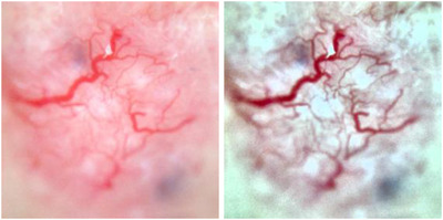
Color augmentations

After the augmentations, we used 3114 images for training and 784 images for validation.

2.3. Image segmentation

We confined the analysis to the BCC by automatic segmentation using U‐Net ¹⁸ with details below.

3. DEEP LEARNING NETWORK

3.1. Network architecture

Biomedical image segmentation often employs U‐Net ¹⁸ due to its ability to perform accurate pixel‐based classification. The network includes contractive and expansive paths where the contractive (encoder) path follows architecture similar to a convolutional neural network and the expansive (decoder) path uses transposed 2D convolutional layers. The encoder is downsampled 4 times and the decoder is upsampled 4 times to restore the high‐level semantic feature map produced by the encoder to the original size of the image (Figure 3).

FIGURE 3.

U‐Net architecture

Each convolutional layer in the encoder part is followed by a maxpool downsampling operation for the network to encode the input image into feature representations at multiple levels. The decoder includes upsampling and concatenation, succeeded by convolution operations. The decoder projects the lower dimensional discriminative features learned by the encoder into a higher‐resolution space. It upsamples the feature map while simultaneously concatenating it with its higher resolution feature map from the encoder part. The final layer does a 1 × 1 convolution to map the last feature map to the respective classes.

Since vessels only constitute about 2–10% of the image, it is essential to use a loss function that addresses this severe class imbalance. We use a combination loss function, a weighted sum of Dice loss and binary cross‐entropy, defined as:

$$\begin{array}{ccc}\hfill DL(y,\widehat{p})& =& 1-(2y\widehat{p}+1)/y+\widehat{p}+1),\hfill \\ \hfill L_{W\mathrm{-}bce}& =& -\frac{1}{\mathrm{N}}\sum _i\beta (y-\log (y))+(1-\beta )(1-y)\log (1-\widehat{y}),\hfill \\ \hfill m(\widehat{y})& =& \alpha L_{W\mathrm{-}bce}-(1-\alpha )DL(y,\widehat{y}),\hfill \end{array}$$

where DL is Dice loss and L_W‐bce is weighted binary cross‐entropy. ¹⁹

We employ U‐Net ¹⁸ with our modifications for vessel segmentation due to its accuracy in pixel‐based classification, as detailed in section 4.

4. EXPERIMENT PERFORMED

Our vessel U‐Net model uses varied input sizes for each of the RGB image channels of 32, 64, 128, 256, and 512. We use Exponential Linear Units activations instead of the traditional U‐Net Relu activations as they tend to converge faster and produce more accurate results. ²¹

$$\begin{array}{c}\hfill F(x)=\left\{\begin{array}{cc}z\hfill & z>0\hfill \\ \alpha .\left(e^z-1\right)\hfill & z\le 0\hfill \end{array}\right\}.\end{array}$$

The weights are initialized from truncated normal distribution centered on zero with standard deviation = sqrt(2/ fan_in), where fan_in is the number of input units in the weight tensor.

To introduce regularization, we use dropout layers with probability 0.1 for both the encoder and decoder. To prevent overfitting, we use early stopping with a patience value of 5 and save the best model. The hyperparameters are listed in Table 1.

TABLE 1.

Different hyperparameters used for training U‐Net

Hyperparameters	Value
One weight	0.89
Zero weight	0.11
Learning rate	0.0001
Epochs	20
Metrics	Jaccard loss
Batch size	8
Alpha for combo loss	0.7

Automatic lesion borders were determined by U‐Net trained on the 2594‐image ISIC 2018 Task 1 Lesion Segmentation data set. ¹⁹ Images were resized to 320 × 320 using bilinear interpolation. We randomly split the images into training and validation set of 80:20. Hyperparameters were similar to Table 1, except the model was trained up to 100 epochs with a batch size of 10 and an Adam optimizer and Dice loss function.

5. EXPERIMENTAL RESULTS

We evaluate our model with the Jaccard (intersection over union) metric. This avoids the overrepresentation of negative pixels in sparse features.

Jaccard Index = $\frac{TP}{TP+FP+FN}(\mathrm{for}\mathrm{binary}$ classification)

Our U‐Net model achieves a Jaccard score of 37.8% on the test set, which exceeds the mean Jaccard score among our 5 observers who created vessel masks. Results of our model are shown in Figure 4 as green overlays, to compare with the predicted masks, white overlays.

FIGURE 4.

Predicted binary masks and overlays

5.1. Vessel detection performance for different loss functions

In this study, 20 epochs yield a stable validation loss (Figure 5).

FIGURE 5.

Training and validation loss curves for combo loss

6. DISCUSSION

We used the basic U‐Net structure of Ronneberger et al. ¹⁸ with modifications as noted in network architecture. We used different loss functions ¹⁹ (Table 2). The mean accuracy, precision, recall, and Jaccard index on the test set for the combination loss function were 0.987, 0.38, 0.574, and 0.521. This compares with mean accuracy, precision, and recall for Kharazmi et al. ¹⁵ of 0.954, 0.947, and 0.917. The latter two scores are higher than we obtained. However, the two studies are not comparable because we score presence or absence of vessels on a pixel‐by‐pixel basis and Kharazmi scores presence or absence of a vessel within a patch of 32 × 32 pixels. Additionally, the Kharazmi masks include vascular structures other than vessels (Figures 5, 6, 7). ¹⁵ Other studies ¹² , ¹³ , ¹⁴ lack pixel‐by‐pixel scoring.

TABLE 2.

Evaluation metrics for different loss functions with U‐Net

Loss functions	Accuracy	Jaccard	Precision	Recall
Weighed BCN	0.98	0.311	0.351	0.734
Tversky loss	0.985	0.351	0.442	0.629
Focal Tversky loss	0.985	0.354	0.435	0.657
Dice loss	0.989	0.364	0.565	0.506
Combo loss	0.987	0.376	0.574	0.521

FIGURE 6.

Mask annotations for the same image by different team members

FIGURE 7.

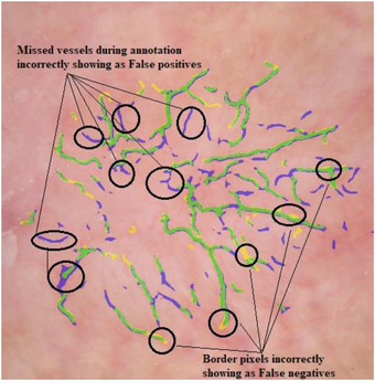
Example of disagreement with manual mask. True positives shown by green, false positives shown by blue and false negatives shown by yellow

To understand our results better, we took samples of 10 random images from each person's mask set and had all 5 observers mark those masks, to create 5 masks for each of the 50 images. One such example of an image and the corresponding mask done by each person is shown below. We can see from the images that there is some difference in the way each person views and draws the vessels.

For the example images shown in Figure 6, the mean Jaccard calculated for each pair of observers on a pixel‐by‐pixel basis for is only 0.285, even though they appear rather similar.

Over the entire set, the median pairwise Jaccard is 0.271. Some of the possible reasons for low Jaccard values are as follows:

1. Interrater variability: The most common variation we observed is the extent of vessel pixel covering, due to inexact fading of the edges of the vessels, and variable covering in the mask. The second most common variation was the varying inclusion of vague vessel structures.

2. Software differences: Two observers used Paint.net and three used Photoshop.

3. Tool variation: For freehand drawing of a mask, variations can also arise from the use of a stylus with Photoshop and a mouse with Paint.net.

Most false positives we observed were the result of blurry or thin vessels missed during mask creation (Figure 7).

This research enables optimal detection of a critical dermoscopy structure in early basal cell carcinoma: thready blood vessels called telangiectasia. We accomplish this vessel segmentation task by combining image preprocessing with U‐Net using our hyperparameters. The study also compares different loss functions and manages class imbalance by using composite loss functions.

The subjective nature of structure identification by different observers has not received sufficient attention in the literature. Accordingly, we present an analysis of differences in vessel detection by different observers. We show that these differences are not a deterrent to accurate detection of these structures. We are able to achieve deep learning results that are more in agreement with each observer than the observers are with each other. In this study, we establish a path to detection of other cancer‐critical signs for earlier cancer detection. In the future, we would like to further explore differences in machine and manual annotation to develop more sophisticated models and different U‐Net approaches. ²⁰ , ²¹

Maurya A, Stanley RJ, Lama N, Jagannathan S, Saeed D, Swinfard S, Hagerty JR, Stoecker WV. A deep learning approach to detect blood vessels in basal cell carcinoma. Skin Res Technol. 2022;28:571–576. 10.1111/srt.13150

REFERENCES

- 1. Rogers HW, Weinstock MA, Feldman SR, Coldiron BM. Incidence estimate of nonmelanoma skin cancer (keratinocyte carcinomas) in the US population, 2012. JAMA Dermatol. 2012;151(10):1081–6. [DOI] [PubMed] [Google Scholar]
- 2. Esteva A, Kuprel B, Novoa RA, Ko J, Swetter SM, Blau HM, Thrun S. Dermatologist‐level classification of skin cancer with deep neural networks, Nature 2017;542(7639):115–8. [DOI] [PMC free article] [PubMed] [Google Scholar]
- 3. Rigel DS, Torres AM, Ely HJ. Imiquimod 5% cream following curettage without electrodesiccation for basal cell carcinoma: preliminary report. J Drugs Dermatol.2008;7(1):15–6. [PubMed] [Google Scholar]
- 4. Marchetti MA, Codella NCF, Dusza SW, Gutman DA, Helba B, Kalloo A, et al. International Skin Imaging Collaboration. Results of the 2016 International Skin Imaging Collaboration International Symposium on Biomedical Imaging challenge: comparison of the accuracy of computer algorithms to dermatologists for the diagnosis of melanoma from dermoscopic images. J Am Acad Dermatol. 2018;78(2):270–7. [DOI] [PMC free article] [PubMed] [Google Scholar]
- 5. Haenssle HA, Fink C, Toberer F, Winkler J, Stolz W, Deinlein T, et al. Man against machine reloaded: performance of a market‐approved convolutional neural network in classifying a broad spectrum of skin lesions in comparison with 96 dermatologists working under less artificial conditions. Ann Oncol. 2020; 31(1):137–43. 10.1016/j.annonc.2019.10.013. [DOI] [PubMed] [Google Scholar]
- 6. Esteva A, Kuprel B, Novoa RA, Ko J, Swetter SM, Blau HM, Thrun S. Dermatologist‐level classification of skin cancer with deep neural networks. Nature. 2017;542(7639):115–8. [DOI] [PMC free article] [PubMed] [Google Scholar]
- 7. Majtner T, Yildirim‐Yayilgan S, Hardeberg JY. Combining deep learning and hand‐crafted features for skin lesion classification. Sixth International Conference on Image Processing Theory, Tools and Applications. (IPTA). Oulu, Finland; 2016. [Google Scholar]
- 8. Codella NCF, Cai J, Abedini M, Garnavi R, Halpern A, Smith JR. Deep learning, sparse coding, and SVM for melanoma recognition in dermoscopy images. International Workshop on Machine Learning in Medical Imaging (MLMI). Munich Germany; 2015. [Google Scholar]
- 9. Codella NCF, Nguyen Q‐T, Pankanti S, Gutman D, Helba B, Halpern A, Smith JF. Deep learning ensembles for melanoma recognition in dermoscopy images. IBM Res Dev. 2017;61(4/5):1–5. [Google Scholar]
- 10. González‐Díaz I. DermaKNet: incorporating the knowledge of dermatologists to convolutional neural networks for skin lesion diagnosis. IEEE J Biomed Health Inform. 2019;23(2):547–59. [DOI] [PubMed] [Google Scholar]
- 11. Hagerty JR, Stanley RJ, Almubarak HA, Lama N, Kasmi R, Guo P, et al. Deep learning and handcrafted method fusion: higher diagnostic accuracy for melanoma dermoscopy images. IEEE J Biomed Health Inform. 2019;23(4):1385–91. [DOI] [PubMed] [Google Scholar]
- 12. Cheng B, Erdos D. Stanley RJ, Stoecker WV, Calcara DA, Gomez DD. Automatic detection of basal cell carcinoma using telangiectasia analysis in dermoscopy skin lesion images. Skin Res Technol. 2011;17(3):278–87. [DOI] [PMC free article] [PubMed] [Google Scholar]
- 13. Cheng B, Stanley RJ, Stoecker WV, Hinton K. Automatic telangiectasia analysis in dermoscopy images using adaptive critic design. Skin Res Technol. 2012;18(4):389–96. [DOI] [PubMed] [Google Scholar]
- 14. Kharazmi P, AlJasser MI, Lui H, Wang ZJ, Lee TK. Automated detection and segmentation of vascular structures of skin lesions seen in dermoscopy, with an application to basal cell carcinoma classification. IEEE J Biomed Health Inform. 2017;21(6):1675–84. [DOI] [PubMed] [Google Scholar]
- 15. Kharazmi P, Zheng J, Lui H, Wang ZJ, Lee TK. A computer‐aided decision support system for detection and locatization of cutaneous vasculature in dermoscopy images via deep feature learning. J Med Syst. 2018;42(2):33. [DOI] [PubMed] [Google Scholar]
- 16. Karimi D, Dou H, Warfield SK, Gholipour A. Deep learning with noisy labels: exploring techniques and remedies in medical image analysis. arXiv 2019; 1–17: 1912.02911. [Online]. Available: http://arxiv.org/abs/1912.02911 [DOI] [PMC free article] [PubMed] [Google Scholar]
- 17. Tschandl P, Rosendahl C, Kittler H. Data Descriptor: the HAM10000 dataset, a large collection of multi‐source dermatoscopic images of common pigmented skin lesions. Sci Data. 2018;5:180161. [DOI] [PMC free article] [PubMed] [Google Scholar]
- 18. Ronneberger O, Fischer P, Brox T. U‐Net: convolutional networks for biomedical image segmentation. [Online]. Available: http://lmb.informatik.uni‐freiburg.de/. Accessed 17 11 2020.
- 19. Jadon S. A survey of loss functions for semantic segmentation, 2020, [Online]. Available: https://arxiv.org/abs/2006.14822. Accessed 17, 11, 2021.
- 20. Codella NCF. Gutman DA, Celebi ME, Helba B. Skin lesion analysis toward melanoma detection 2018: a challenge hosted by the International Skin Imaging Collaboration (ISIC). arXiv:1902.03368 [cs.CV]; 2019. Available: https://arxiv.org/abs/1902.03368. Accessed 17, 11, 2021. [Google Scholar]
- 21. Oskal KRJ, Risdal M, Janssen EAM, Undersrud ES, Gulsrud TO, et al. A U‐net based approach to epidermal tissue segmentation in whole slide histopathological images. SN Appl Sci. 2019; 1:672. [Google Scholar]