

Abstract
Based on data on school visits from Safegraph and on school closures from Burbio, we document that during the Covid-19 crisis secondary schools were closed for in-person learning for longer periods than elementary schools, private schools experienced shorter closures than public schools, and schools in poorer US counties experienced shorter school closures. To quantify the long-run consequences of these school closures, we extend the structural life cycle model of private and public schooling investments by Fuchs-Schündeln et al. (Econ J 132:1647–1683, 2022) to include private school choice and feed into the model the school closure measures from our empirical analysis. Future earnings and welfare losses are largest for children that started public secondary schools at the onset of the Covid-19 crisis. Comparing children from the top to children from the bottom quartile of the income distribution, welfare losses are 0.5 percentage points larger for the poorer children if school closures were unrelated to income. Accounting for the longer school closures in richer counties reduces this gap by about 1/4. A policy intervention that extends schools by 6 weeks generates significant welfare gains for children and raises future tax revenues sufficient to pay for the cost of this schooling expansion.
Keywords: Covid-19, School closures, Inequality, Intergenerational persistence
Introduction
Governments around the world responded to the Covid-19 health crisis by shutting down economic and social activity, resulting in severe recessions and closed schools for much of 2020. The economic consequences of these lockdown measures triggered a large scientific and popular literature. As many countries are on the path of economic recovery from this crisis, focus is shifting from the short- to the long-run consequences of the crisis. One such concern is the long-run impact of the significant loss of instructional time in schools during 2020–21 on children’s education, earnings potential and future welfare.
In this paper, we use a structural life-cycle model and school visit measures from anonymized cell phone data combined with learning mode data to quantify the heterogeneous impact of school closures during the Covid-19 crisis on children affected at different ages and coming from households with different socio-economic parental characteristics. Our data suggests that secondary schools were closed for in-person learning for longer periods than elementary schools, implying that younger children experienced shorter school closures than older children, and that private schools1 experienced shorter closures than public schools, and schools in poorer US counties experienced shorter school closures. We use these empirical facts as inputs for a positive and normative analysis of the long-run consequences of the observed Covid-19-induced school closures on the affected children. To do so, we extend the structural life cycle model of schooling investments studied in Fuchs-Schündeln et al. (2022) to include the choice of parents to send their children to private schools, empirically discipline it with data on parental investments from the PSID, and then feed into the model the school closures measures from our empirical analysis to quantify the aggregate and distributional consequences of the Covid-19 school closures.
We highlight two main findings. First, the aggregate losses of human capital, college attainment, the present discounted value of earnings and welfare are large: the present discounted value (PDV) of future gross earnings (after the current school children enter the labor market) falls by 1.27% and the welfare losses amount to 0.71% of permanent consumption. These results materialize despite the fact that parents optimally adjust their private time- and resource investment into their children, as well as inter-vivos transfers of wealth to their offspring.
Second, if all children had their schools closed for the same amount of time, then younger children, and those from disadvantaged backgrounds would suffer larger welfare losses, as our previous work suggested.2 However, due to the significant empirically documented differences in the extent of the school closures, these conclusions are partially overturned, and partially accentuated. The fact that, on average, secondary schools were closed much longer than primary schools leads to the finding that it is children just starting secondary school that endure the largest losses in their earnings capacity (a reduction of the PDV of earnings of approximately 1.5%) and welfare (a decline of 0.83%).
Turning to socio-economic characteristics, we make two empirical observations. First, private schools were closed on average for fewer days than public schools, and private schools are dis-proportionally frequented by children from parents with higher socio-economic characteristics (in the model, associated with higher education, higher wealth and being married). However, focusing on only public schools, these were closed for longer in counties with higher average income.
The quantitative model maps these empirical findings into expected differential welfare consequences. Children attending private schools on average lose points less welfare (measured in terms of permanent consumption), than children attending public schools, accentuating the larger welfare losses poorer children have in the absence of differential school closures. Within public schools, however the income gradient of welfare losses goes in the opposite direction since poorer areas in the USA, especially in the South but also the Midwest, saw shorter school closures on average than the more affluent regions on both coasts. Of course, children from poorer households are still worse off and might have been affected more severely from the Covid-19 crisis along many other dimensions, but the fact that, again on average, their schools were locked for shorter periods of time than the schools in richer counties implies that the losses in human capital, lifetime earnings, and ultimately, welfare, are more benign than those children from richer families (or more precisely, residing in richer counties).
Finally, and motivated by the significant and heterogeneous human capital and welfare losses we consider potential policy interventions designed to mitigate the instructional losses from the Covid-19 crisis. One such proposal is to keep schools open for parts of future summer periods to make up the lost time. In the model, since we have a well-defined cost of schooling and model-predicted consequences of additional schooling on future human capital, earnings and taxes, we can ask whether such a measure is a positive net present discounted value proposition for households. Furthermore, since a policy intervention that keeps all schools open might not be feasible due to scarcity in the availability of teachers or physical infrastructure, we also investigate for which group of students such a policy intervention is especially promising, both in terms of the budgetary consequences for the government and in terms of welfare for the individual students. We find that for the average child the welfare gains from expanded schooling are significant (0.22% in terms of consumption equivalent variation), and induce an increase in future revenues from labor income and consumption taxes approximately sufficient to pay for the entire cost of the reform; that is, the reform is essentially budget-neutral. Finally, the welfare gains from the expansion are highest for children from income-poor households, whereas the fiscal consequences for the government look most favorable if the intervention is targeted to children from the most affluent households.
In the next section, we briefly relate our model to the existing literature. Section 3 describes the data we use to construct measures of school closures and the empirical measures of school closures we will employ in the structural model. That model is spelled out in Sect. 4 and calibrated in Sect. 5. We present the results on the differential welfare consequences of the school closures in Sect. 6, and Sects. 7 and 8 contain the counterfactual policy analysis and robustness analysis, respectively. Section 9 concludes. Details about the construction of the data as well as the dynamic programs in the model can be found in Appendix.
Related Literature
Our paper is part of the massive literature on the consequences of the Covid-19 epidemic on the economy. The early literature focused on short-run predictions of the evolution of the health crisis and the economic recession, triggered by a fall in the healthy work force and its desire to work in risky sectors, the demand for goods and services induced by falling household incomes as well as massive government-mandated economic lockdowns. Representative contributions include Atkeson (2020), Fernandez-Villaverde et al. (2020), Greenstone et al. (2020) and Alemán et al. (2021) on the health side and Eichenbaum et al. (2020) as well as Krueger et al. (2020), Moll et al. (2020) on the economic side. A subset of this literature (see, e.g., Argente et al. (2020), Acemoglu et al. (2020), Glover et al. (2020), Brotherhood et al. (2020)) has considered optimal lockdown policies, where the main benefit of shutting down part of the economy is a slower transmission of the virus, and the main cost is modeled as the reduction of economic activity and thus incomes of individuals of current working age. The paper by Ma et al. (2022) makes the important point that the impact of the economic contraction on child mortality, especially in developing economies, can be so severe to render lockdown measures counterproductive for protecting the lives of children. The potential impact of closing schools as part of the lockdown is not considered in this literature.
Complementary to this work, our paper takes a longer-run perspective and analyzes the consequences of one specific aspect of the crisis, school closures, that initially did not receive much attention, likely due to the fact that the main costs associated with this non-pharmacological intervention accrue mostly in the medium to long-run when the cohort of school children affected by school closures enter the higher education- or labor market. In our previous work (Fuchs-Schündeln et al. 2022) we used a structural life cycle model to quantify the impact of a hypothetical school closure for 12 months on average human capital accumulation, lifetime earnings and welfare. In the current paper we build on this framework, but turn to school visits data from Safegraph and information on school learning modes from Burbio to measure the actual length of school closures. Crucially, we argue that there is significant heterogeneity across school types (public versus private), grade level (elementary versus secondary), and parental backgrounds in the extent to which schools were closed. This analysis is motivated by an emerging body of evidence that learning achievement during the pandemic was substantially lower than in prior years, suggesting that the virtual instruction brought about by school closures was much less effective than traditional in-person instruction.3
Therefore, the main contribution of the current paper is to develop a new measure of effective school closures using Safegraph school visits data and employ it in a structural life cycle model with human capital accumulation to quantify the long-run earnings and welfare consequences of the affected children. On the empirical side, the Safegraph visits data has been used by other studies to measure social distancing behavior, the impact of the pandemic on in-person services, and industry affiliation of particular businesses (e.g., Allcott et al. (2020), Goolsbee and Syverson (2021), or Kurmann et al. (2021) among many others). The papers closest to ours are Chernozhukov et al. (2021) and Bravata et al. (2021) who estimate the association between changes in Safegraph visits to schools and the spread of Covid-19 at the county level, as well as Parolin and Lee (2021) who use the Safegraph data to construct a school closure index and, like us, match the Safegraph data with information from NCES and other sources to relate their school closure index to grade level (elementary versus secondary) and a variety of socioeconomic indicators.4 Different from these papers, we build on the approach by Kurmann and Lalé (2021) and combine the Safegraph visits data with data on learning modes by Burbio to estimate a mapping of changes in school visits to in-person schooling time. This allows us to construct a measure of effective schooling time by school type (public versus private school), grade level, and parental background, which in turn constitutes a crucial input for our model simulations.5
On the modeling side, we take a structural approach to answer our applied policy question, building on the literature modeling human capital accumulation in children of school age and public education, see, e.g., Cunha et al. (2006), Cunha and Heckman (2007), Cunha et al. (2010), Caucutt and Lochner (2020), Kotera and Seshadri (2017), Lee and Seshadri (2019), Yum (2020), Caucutt et al. (2020), Daruich (2022), Morchio (2022), Jang et al. (2021) and especially Agostinelli et al. (2020). A complementary, more empirically oriented literature, assesses the importance of instruction time or schooling inputs for student outcomes, see, e.g., Lavy (2015), Carlsson et al. (2015), Rivkin and Schimann (2015), Fitzpatrick et al. (2011), Pischke (2007),Jaume and Willén (2019), Werner and Woessmann (2021) and Maldonado et al. (2021).6
Data
In this section, we describe the data and procedures to measure effective schooling time during the pandemic. We start with the Safegraph data, how we measure changes in visits to schools, and how we match the schools with records from the National Center for Education Statistics (NCES) to obtain information on different school characteristics. Then, we show how we use Burbio data on school learning modes to map changes in school visits to total in-person learning and effective schooling time. Finally, we present the empirical results that serve as input for the structural model simulations.
Measuring In-person Learning
Safegraph School Visit Data
The first source of information for measuring in-person learning comes from Safegraph, which provides data for over 6 million Places of Interest (POIs) for the USA using cell phone pings.7 From this large set of POIs we extract establishments with North American Industry Classification System (NAICS) code 611110 (“Elementary and Secondary Schools”) that are present in Safegraph’s Weekly Patterns, which provides data on weekly visits by POI. We then match Safegraph’s POIs with NAICS code 611110 by school name and address to public and private schools from the Department of Education’s National Center for Education Statistics (NCES), resulting in about 102,500 high-quality matches of schools with Safegraph data on weekly visits. Appendix B provides details of the matching procedure and results. Relative to the universe of schools in the NCES, we lose about 22,000 schools, but the matched school sample remains highly representative of the overall population of schools in terms of socioeconomic and geographic makeup.
Measuring Changes in School Visits
The Safegraph data provide weekly visit counts for each school by dwell times. There are dwell time intervals (less than 5, 5 to 10, 11 to 20, 21 to 60, 61 to 120, 121 to 240, more than 240 minutes), Denoting weekly visits counts as for , the total visits count for school j in week t is
As Fig. 4 in Appendix shows, prior to the pandemic, both aggregate total visit counts and aggregate visits longer than 240 minutes per day decline markedly during the weeks of Thanksgiving, Christmas, and Summer break. In addition and in line with the public health emergency declared on March 13, 2020, both visits series drop precipitously during the week of March 15 to March 21, 2020, and remain substantially lower thereafter.
Fig. 4.

Aggregate time series of visits (week 1 = 1st week of 2020)
We construct changes in school visits as the dwell-time weighted growth rate in visits relative to average visits prior to the pandemic. This measure, which is different from Chernozhukov et al. (2021), Bravata et al. (2021), and Parolin and Lee (2021) who instead consider year-over-year changes in visits, has the advantage that it is not affected by holidays and other variations in visits that fall on different weeks across years, thereby reducing measurement error. Furthermore, we normalize weekly visits for each school by the county-level count of cell phone devices in the Safegraph data so as to control for spurious variations in school visits due to changes in sample coverage.8 The construction of our measure of school visit changes involves three steps:
- For each school j, we define weights as:
where denotes the base period (November 2019 through the end of February 2020, excluding the weeks of Thanksgiving, Christmas and New Year); and measures the contribution of a dwell time d to school j’s raw visits counts during the base period. - Using the weights, we measure weighted weekly visits at school j in week t as
where denotes the normalization by SG devices during week t in county in which the school j is located. - Given weighted and normalized school visits, we measure the change in school visits as
where is the mean value of during the base period.
In order to further reduce measurement error, we top-code at 100%. In addition, if in any week t outside of the base period while and , we replace by the average of and . This adjustment implements the assumption that during the school year 2020–21, schools did not reopen for only one week at a time. Finally, we drop about 30,000 schools with sparse or very noisy visit data, and apply weights to ensure that the remaining sample of roughly 70,000 schools remains representative of the full sample of schools in the USA. See Appendix B.1 for details on the sample selection criteria and weighting procedure.
Figure 1 presents histograms of the distribution of changes in school visits during three subperiods (averaged over the weeks within a subperiod). The figure shows that relative to the pre-pandemic period, school visits declined massively during March–May 2020, and were still significantly lower during September–December 2020 and (less so) during January–May 2021.
Fig. 1.

Distribution of changes in school visits for selected subperiods
Figure 2 shows the geographical variation in county average school visit changes for the three subperiods. During March–May 2020, school visits were 75 to 100 percent below pre-pandemic levels, without much regional variation. During September–December 2020, in contrast, we observe substantial variation in school visits across different regions, as many schools in the Southern, Midwestern, and Central Northern parts of the USA reopened while schools in the Western and Eastern parts remained largely closed. During January–May 2021, the situation becomes again more even, with school visits returning toward pre-pandemic levels in most counties except on the West Coast, parts of the East Coast, and a few other counties across the USA.
Fig. 2.
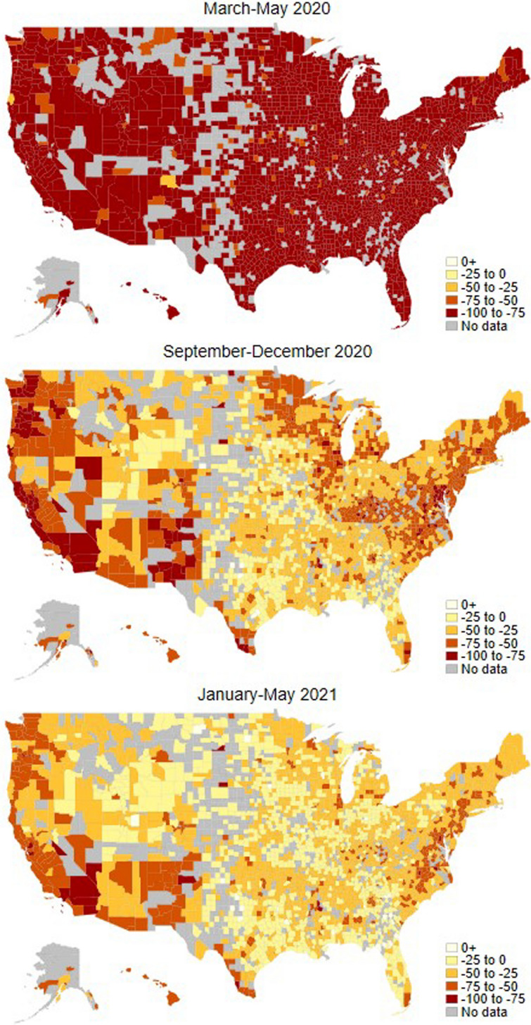
Average Change in School Visits by County: March–May 2020
From Changes in School Visits to In-person Learning
While the Safegraph data provide us with a high-frequency measure of changes in school visits for a large, representative sample of public and private schools, it is not clear what a given decline in school visits represents in terms of lost in-person learning. To map changes in school visits into a measure of in-person learning, we relate our school visit data to estimates of school learning mode from Burbio. Burbio is a private company that collects data for 1200 public school districts representing 47 percent of USA. K-12 student enrollment in over 35,000 schools in all 50 states. The data is aggregated to the county level and primarily used for commercial purposes, but the company generously shared the data with us and other researchers. The information on learning mode consists of weekly indicators between mid-August 2020 and mid-June 2021 that for each county provide the percent of public school students engaged in a traditional, a hybrid, or a virtual learning mode. Traditional means that students attend in-person school every day of the week; hybrid means that students attend 2–3 days per week in-person; virtual means that students do not attend school in person. Appendix B.2 contains details about the Burbio data.
To construct the mapping, we start by computing county-level averages of the fractions that public school students spent in learning mode between week and week from the Burbio data, i.e.,
| 1 |
where denotes the percent of students in county c who spent week t in learning mode L; and is the number of weeks considered. For instance, for computed from September 2020 to June 2021 means that public school students in county c spent one third of the school year 2020–2021 in traditional learning mode.
Next, we define the fraction of the school year that students in county c effectively spent in in-person learning mode as and the fraction effectively spent in virtual learning mode as , where measures the fraction of total student-days that are spent in person when the learning mode is hybrid. We then relate these measures to the change in Safegraph school visits with the following linear regression
or equivalently,
| 2 |
where is the student-weighted average of changes in school visits across schools in county c. The regression tells us not only how a given change in school visits maps into total in-person learning relative to its pre-pandemic level, , but also the average proportion of in-person learning when students are in hybrid mode. Since , the regression also tells us how a given change in school visits maps into total virtual learning .
We estimate (2) using Burbio and Safegraph data for Fall 2020 only. The reason we do not use data for Winter and Spring 2021 is that during this period, school districts increasingly moved away from virtual learning. As a result, changes in traditional learning are close to linear with hybrid learning . In a regression, this implies and since is subject to idiosyncratic noise. During Fall 2020, in contrast, there are changes across all three learning modes, which enables us to identify the mapping between and , controlling for .
Table 1 reports the results of the estimation. In column (1), we consider all counties for which we have data on both Burbio learning modes and Safegraph school visits (3049 out of 3124 available counties in Burbio). The sample represents almost 95 percent of all public-school students in the USA. The mapping between the different variables is tightly estimated, with a of over 0.5 and highly significant coefficients. A 1 percentage point decline in school visits reduces the average fraction of weeks spent in traditional learning mode by 1.14 percentage points, and the estimated average fraction of hybrid learning mode spent in in-person learning mode is 0.5 or 2.5 days out of a 5 day school week. Furthermore, we verify using a nonparametric binned scatter plot that over the range of school visit changes observed, the resulting relationship between total in-person learning and the change in school visits is indeed well represented by a linear function. Finally, the estimated intercept is 101.67, close to the predicted value of 100 when school is fully in-person (i.e., and ).
Table 1.
Regression of traditional learning against changes in school visits
| Dependent variable: Traditional (in-person) learning mode | ||||
|---|---|---|---|---|
| (1) | (2) | (3) | (4) | |
| Change in school visits | 1.14*** | 1.12*** | 1.13*** | 1.15*** |
| (0.04) | (0.04) | (0.04) | (0.05) | |
| Hybrid learning mode | − 0.50*** | − 0.49*** | − 0.48*** | − 0.43*** |
| (0.02) | (0.03) | (0.03) | (0.03) | |
| Intercept | 101.67*** | |||
| (2.51) | ||||
| Adjusted | 0.513 | 0.513 | 0.522 | 0.589 |
| N of counties | 3049 | 3049 | 2438 | 794 |
| N of students (in thousands) | 48,013 | 48,013 | 47,250 | 40,485 |
| % of all public-school students | 94.5 | 94.5 | 92.9 | 79.6 |
Safegraph and Burbio data are averaged at the county level for Fall 2020 (weeks of September 27–October 3 to December 13–December 19, excluding the week of Thanksgiving). All regressions are weighted by county-level student enrollment and standard errors (in parenthesis) are clustered at the state level. In columns (2)–(4) the intercept is constrained to 100
As robustness checks, in column (2) we restrict the intercept to 100 and rerun the regression, while in columns (3) and (4), we reduce the sample to the counties with at least 5 schools for which we have data, respectively, to the counties in the top-25 percent of the population distribution. The results are strikingly robust across the different specifications: a 1 percentage point decline in school visits reduces the fraction of weeks spent in effective in-person learning by 1.14 percentage points, and hybrid learning mode is estimated to correspond to a fraction of 0.43 to 0.49 of in-person learning mode.
In sum, the regressions confirm that there is a tight linear relationship between change in school visits and effective in-person learning. We therefore feel confident to use this mapping to infer effective schooling time at the individual school level.
Effective Schooling Time by School Characteristic
In the model simulations below, effective schooling time over the two-year period between Summer 2019 and Summer 2021 will be an important input to quantify the consequences of learning loss during the pandemic. We proceed as follows to infer this value from our estimates of in-person learning. According to the NCES table of “Number of instructional days and hours in the school year” (https://nces.ed.gov/programs/statereform/tab5_14.asp), there are 180 instructional days per year in almost every state. Dividing this number by 5 (since weekends are excluded from the counts), we obtain 36 weeks of potential schooling per year.9 Equivalently, we have 72 weeks of potential schooling for the two-year period between Summer 2019 and Summer 2021. For the 25 weeks between September 2019 and mid-March 2020 that precede the pandemic, we set effective school time to 100 percent. For the remaining 11 weeks of the 2019–2020 school year (week of Mar 15–Mar 21 through the week of May 24–May 30) and the 36 weeks of the 2020–2021 school year, hence for weeks, we calculate effective schooling time using the estimates in Table 1 as follows. For a set of schools with a certain characteristic s (e.g., public vs private schools), we take the average student-weighted change in school visits and calculate effective schooling time as , where , , and denotes the effectiveness of virtual learning. Thus, our estimate of effective schooling time – what we will call schooling input in the model-based analysis – during the two-year period from 2019 to 2021, as a percent of what schooling time would have been without the pandemic, is
| 3 |
The equation makes clear that schooling input depends importantly on the effectiveness of virtual schooling . While empirical evidence is accumulating that virtual instruction was a highly imperfect substitute for in-person instruction, pinning down how much less effective exactly virtual instruction was for the average student is a non-trivial task.
The most direct way to determine , and the one we follow for our benchmark result, is to use empirical studies that directly measure the loss in schooling inputs from test score declines. Dorn et al. (2021) find, based on data from Curriculum Associates, a standardized test provider, that by the end of the 2020–21 school year, public school students in grades 1–6 were on average 5 months behind in mathematics relative to their pre-pandemic peers. Under the assumption that lost effective schooling time translates one-to-one into learning loss, then based on (3), this implies a value for the effectiveness of virtual learning of , the benchmark value we use.
On the one hand, this value of may overstate the effectiveness of virtual learning both because of selection due to higher rates of absenteeism and declines in enrollment of lower-achieving students, and because many parents compensated for the loss of in-person schooling by taking over some of the instructional duties of teachers or paid tutors to do so (as they will in our model). On the other hand, students may also have been negatively affected by pandemic disruptions not directly related to schooling (e.g., health issues, job loss in the family), which would imply learning losses even if virtual schooling was highly effective.
Anticipating model simulation results below, we find that with a value of , we obtain an average learning loss of about 8.5% over the 2-year Covid period, while with a value of , we obtain a learning loss of about 12%. Both of these values are considerably smaller than the estimated average learning losses by Dorn et al. (2021), suggesting that disruptions not directly related to schools (and not taken into account by our model) indeed exerted a non-negligible negative impact. To make further progress, we contrast our simulation results with empirical studies such as Goldhaber et al. (2022) that seek to estimate pandemic learning loss directly as a function of instructional mode while controlling for regional differences in pandemic health and economic outcomes as well demographic and socio-economic characteristics of students. Their results imply that relative to students who attended school mostly in-person, learning loss was about twice as large for students who were primarily in virtual mode than for students who were primarily in hybrid mode.10 This suggests that the effectiveness of virtual learning was indeed low for the average student. We therefore consider a conservative assumption, and appears as a plausible alternative whose consequences we explore in Sect. 8.1.
Table 2 shows lost effective schooling time by school characteristics under the two different assumptions about the effectiveness of virtual learning. Across all schools in the sample, school visits declined by a student-weighted average of over the period from mid-March 2020 through the end of the 2020–21 school year. Using the average of the coefficient estimates in columns (2) and (4) of Table 1, this implies total in-person learning of about during that period and total virtual learning of about .
Table 2.
Estimates of effective schooling time over the 2019–2021 period
| All | Elementary | Secondary | |
|---|---|---|---|
| With virtual learning at 25% effectiveness | |||
| All | 69.4 | 71.7 | 64.2 |
| [68.7, 70.1] | [71.0, 72.3] | [63.4, 65.0] | |
| Private schools | 74.4 | 74.7 | 71.6 |
| [73.9, 75.0] | [74.1, 75.2] | [70.9, 72.2] | |
| Public schools, all | 68.9 | 71.5 | 63.8 |
| [68.2, 69.6] | [70.8, 72.1] | [63.0, 64.6] | |
| Public schools, top-25% income | 65.9 | 68.5 | 60.1 |
| [65.1, 66.6] | [67.8, 69.2] | [59.2, 61.0] | |
| Public schools, bottom-25% income | 72.9 | 74.9 | 68.6 |
| [72.3, 73.5] | [74.4, 75.5] | [67.9, 69.3] | |
| With virtual learning at 0% effectiveness | |||
| All | 59.2 | 62.2 | 52.3 |
| [58.3, 60.1] | [61.4, 63.1] | [51.2, 53.3] | |
| Private schools | 65.9 | 66.2 | 62.1 |
| [65.2, 66.7] | [65.5, 67.0] | [61.2, 62.9] | |
| Public schools, all | 58.5 | 62.0 | 51.7 |
| [57.6, 59.5] | [61.1, 62.8] | [50.6, 52.8] | |
| Public schools, top-25% income | 54.5 | 58.0 | 46.8 |
| [53.5, 55.5] | [57.1, 58.9] | [45.6, 48.0] | |
| Public schools, bottom-25% income | 63.9 | 66.6 | 58.2 |
| [63.1, 64.7] | [65.9, 67.3] | [57.2, 59.1] | |
The upper panel reports the share of effective schooling time for the 2019–2021 period as a percent of what schooling time would have been without the pandemic under the assumption that virtual learning was 25% as effective as in-person learning. The lower panel reports the share of effective schooling time under the assumption that virtual learning was not effective (i.e., the figures correspond to the share of potential schooling time over the 2019–2021 period that was effectively spent in the classroom). In each cell, the bracketed numbers correspond to lower and upper bounds based on the Burbio estimates reported in Table 1, and the point estimate is computed as the mid-point of the interval
For the baseline case of effectiveness of virtual learning, effective schooling time over the two-year period over the 2019–20 and 2020–21 school years therefore equals about
relative to a situation with full in-person learning. This value is shown in the top-left corner of the first panel of Table 2. If instead, virtual learning had effectiveness, the implied effective schooling time equals , as shown in the top-left corner of the second panel of Table 2.
The remainder of the table reports results of the same calculations separately for private versus public schools and for elementary versus secondary schools. Private schools experienced on average smaller declines in school visits during the pandemic than public schools. Similarly, elementary schools experienced smaller declines in school visits than secondary schools (either private or public, although for public schools the difference between elementary and secondary schools is larger). As a result, effective schooling time during the pandemic is estimated to have been highest for private elementary schools and lowest for secondary public schools.
The last two rows of each panel dig deeper into differences across public schools by looking separately at schools located either in a county ranked in the top or the bottom quartile of the national household income distribution. Perhaps surprisingly, public schools in affluent counties experienced on average a larger decline in school visits and therefore lower effective schooling time during the pandemic than public schools in less affluent counties. As shown in separate work by Kurmann and Lalé (2021), this difference is primarily due to the fact that the affluent counties are disproportionally located in states where schools did not return to full in-person instruction for a large part of the 2020–21 school year. Within quartiles of average household income, the difference in effective schooling time between elementary and secondary schools remains similar as reported in Table 2.
To sum up, the results in this section reveal large differences in total in-person schooling across different types of schools. Under what we argue are reasonable assumptions about the effectiveness of virtual schooling, this implies substantial variations in effective schooling time, i.e., schooling input. In the model simulations that follow, we will exploit these variations in schooling input to analyze the extent to which they result in heterogeneous earnings- and welfare losses for children in different school types, grades, and with different household income.
A Quantitative Life Cycle Model with Education Choices
We now describe the structural life cycle model that we will employ to measure the heterogeneous consequences for lifetime earnings, welfare, and taxes paid of the school closures we measured empirically in the previous section. We first describe the demographics, timing, stochastic structure, endowments, preferences and government policy and then formulate the individual decision problems recursively, since this is the representation we will compute. Since this model shares many features with the one used in Fuchs-Schündeln et al. (2022) we will focus on the novel features relative to their model when presenting the recursive representation of the model, relegating a complete account of all other dynamic programming problems of the model to Appendix A.
Individual State Variables, Risk, and Economic Decisions
We model individuals living in discrete time and denote the current period by t. Ours is a partial equilibrium model where individuals of two generations, a parent generation and a children generation, live through a full life cycle. When children live in the parental household, the key education investment decisions (whether to send the child to private or public school, and how much time and resources to invest into the child during her schooling years) are being taken by parents. The child generation makes one key decision upon becoming an independent household: equipped with inter-vivos transfers of the parent it decides what tertiary education, if any, to attain. After this decision this generation lives through a standard consumption-saving life cycle model; the same is true for the parental generation after the children have left the household. The timing and events in the model are summarized in Fig. 3. We now turn to a detailed description of the underlying heterogeneity of individuals and of each phase of the life cycle they undergo.
Fig. 3.

Life-cycle of child and parental households
Individuals are part of either the child or parental generation, . They differ in their marital status for single and married, their age , where a model period and age j spans two years in real time, their asset position a, their current human capital h, their education level for no higher education (no high school completion), high school attendance and completion, college attendance and completion, and idiosyncratic productivity risk modeled as a two state Markov process with state vector , where is low and is high labor productivity, and transition matrix and initial distribution as well as a transitory shock drawn from distribution . Parents decide in each period to send their children either to public or private school, . All individual state variables and the range of values they can take are summarized in Table 3.
Table 3.
State variables
| State Var. | Values | Interpretation |
|---|---|---|
| k | Generation | |
| m | Marital status | |
| j | Model age | |
| a | Assets | |
| s | School type | |
| h | Human capital | |
| e | Education | |
| Persistent productivity shock | ||
| Transitory productivity shock |
This table lists the state variables of the quantitative model
Demographics
Parents give birth to children when they are of age . The number of children a parental household has differs by marital status m and educational attainment of the parents e. There is no survival risk and all households live until age J. Therefore the cohort size within each generation remains constant over time. We now describe in detail how life unfolds first for parents and then for children, as summarized in Fig. 3.
Life of the Parental Generation
In the model, parental households start their economic life at age just before their children are born. Their initial characteristics include their exogenous marital status m, education level e, initial idiosyncratic productivity states and and initial assets a. These initial states are exogenously given to the household, and drawn from the population distribution which are derived directly from the data, as described in the calibration section.
Parents observe the innate ability (initial human capital) of their children at child model age (real biological age 4), which depends on parental education e and marital status m. Children live with their parents until child age (parental age ), at which point they leave the household to form their own independent household. During these years (parental ages ), parents invest resources and time into their children. For all ages of the child ( is real biological age 6), parents further decide in each period whether to send their children to a public or a private school, , trading off the cost of private school tuition with higher productivity in the human capital production function and thus higher human capital (and associated higher chance of attending college) as well as ultimately, higher expected earnings of their children. If parents opt for private school, then they pay private school tuition , which depends on a child’s age j because we distinguish between tuition for primary and secondary education.11 Attendance in public schools is free, . Kindergarten at child age and school type determines the schooling investment which together with the resource and time investments determines the evolution of a child’s human capital. As a result of these choices, the human capital of a child during school ages evolves according to
| 4 |
where g is a function of the child’s age j (to reflect age differences in the relative importance of education inputs) as well as a function of the school type s (to reflect potential productivity differences across the two school types), and depends positively on the three inputs (parental resources , parental time and schooling input ). To give the human capital accumulation technology a clearer interpretation, from the perspective of the model, h will be useful because it decreases the utility cost of succeeding in high school and college and it increases earnings conditional on a given tertiary education level. Thus, our notion of human capital should be interpreted as broad, including all cognitive and non-cognitive skills that contribute to tertiary schooling success and is rewarded through higher earnings in the labor market.
When children leave the household at parental age , their parents may give them inter-vivos transfers . This is the final interaction between parents and children, after which the two households separate. Parents also make the private school choice on behalf of their children with which the latter start their independent life. Thus, parental transfers to children for whom the parents choose private school have to be at least as high as the school fees, thus .
The remainder of parental life then unfolds as a standard life cycle model. Throughout their working ages, parental households spend an exogenous amount of time on market work which differs by marital status. Labor productivity and thus individual wages are determined by an exogenous productivity profile that depends on household age j, education e, marital status m, and is impacted by the persistent shock and the transitory shock . Labor income of parents of age j, education e and marital status m and hit by shocks is then given by
| 5 |
In addition to making human capital investment decisions for their children when these are present in the household, parents in each period make a standard consumption-saving choice, subject to a potentially binding borrowing constraint , which will be parameterized such that the model replicates well household debt at the age at which households have children . The borrowing limits decline linearly to zero over the life cycle toward the last period of work. Parents work until retirement at age , at which point they start to receive per-period retirement benefits until the end of life at age J. Table 4 summarizes the choices of parents described thus far, and those of children, to which we turn next.
Table 4.
Per period decision variables
| Dec. Var. | Values | Decision period | Interpretation |
|---|---|---|---|
| c | Consumption | ||
| Asset accumulation | |||
| s | School Type | ||
| Time investments | |||
| Monetary investments | |||
| b | Monetary inter-vivos transfer | ||
| e | (Higher) education |
This table lists the decision variables of the economic model
Life of the Children Generation
Children born at age are economically inactive for the first periods of their life. A child’s human capital during ages evolves as the outcome of parental investment decisions described above and schooling input . At the beginning of age and based on both the level of human capital as well as the financial transfer b from their parents (which determines their initial wealth a), children make a discrete higher education decision , where stands in for the choice not to complete high school, hs for high school completion, and co for college completion, respectively. For simplicity, children are stand-in bachelor households through their entire life-cycle.
Acquiring a high school or college degree comes at a utility cost (psychological cost) , which is decreasing in the child’s acquired human capital h and also depends on parental education as well as on whether the student attended private or public school, . In addition, college education requires a monetary cost . Children may finance some of their college expenses by borrowing, subject to a credit limit given by , which is zero for i.e.. for individuals not going to college. As was the case for parents, this limit decreases linearly with age and converges to zero at the age of retirement requiring the children generation to pay off their student loans prior to their retirement.
Youngsters who decide not to complete high school, , enter the labor market immediately at age . Those who decide to complete high school, but not to attend college, do so at age . While at high school, , they work part-time at wages of education group , and those children attending a private high-school also have to pay the school tuition . Those youngsters who decide to attend college enter the labor market at age and also work part-time at wages of education group during their high-school and college years
When the children generation enters the labor market (either without a high-school diploma, with a high-school degree or with a college degree), the acquired human capital during the school years is mapped into an idiosyncratic permanent labor productivity state , which is increasing in acquired human capital h and also positively depends on education e to reflect differential complementarities between education and human capital in generating earnings. When starting to work, children also draw the persistent productivity shock , which follows the same first-order Markov chain as for the parental generation, and stochastic transitory productivity . Labor income of children during the working period is then given by
We restrict attention to the two generations directly impacted by the Covid-19 school crisis, and thus assume that the child generation does not have offspring of their own. As a consequence the remaining decision problem of the child generation, after labor market entry, constitutes a completely standard life-cycle consumption-saving problem.
Recursive Formulation of the Decision Problems
Our model is a partial equilibrium model where the only interaction of the decision problems comes in the period in which the children generation leaves the household. Furthermore, children do not make economic decisions prior to that period. We can therefore solve the entire model backward, starting from the retirement phase of the children generation. The details of those recursive problems not spelled out explicitly in the main text are contained in Appendix A.
Children
The children generation undergoes three distinct phases, first making the education decision, and then living through a working phase and a retirement phase with which we begin.
The Retirement Phase During the retirement phase, at ages , the children generation solves a standard consumption-saving maximization problem, facing a typical budget constraint of the form:
where is pension income, whose dependence on (the persistent income state in the period prior to retirement), education e and human capital h captures the progressive nature of the social security system in past earnings, which are in turn determined by . The function represents a progressive labor income tax code, and capital and consumption are taxed at proportional rates . The associated value function at the time of retirement is given by with .
Working Life Let denote the value function of a children household (assumed to be single) aged j that has entered the labor market with education level e, human capital h and has received stochastic income shocks . This value function is the result of a standard consumption-saving maximization problem, as for retired households, but with budget constraint now given by
Here is taxable labor income, with being the social security payroll tax. The argument of the tax function T encodes that employer contributions to social security are not taxable income. In addition to the budget constraint, the household faces an age-, education, and generation-specific borrowing limit .
The Higher Education Choice The key choice of the children generation impacted by the Covid-19 crisis and associated loss in schooling is the higher education decision this generation will make in the model right after the establishment of an independent household, and after having received inter-vivos transfers from their parents. 16-year-olds have three discrete choices : they can either decide to drop out of high school and enter the labor market directly at age 16, or complete high school prior to labor market entry at age 18, or third, go to and complete college at age 22 prior to labor market entry. To spell out this higher education decision problem, we first have to specify the values from each of these three discrete options.
Dropping Out of High School Members of the children generation that made the decision to drop out of high school at model age (real age 16), i.e., chose , directly enter the labor market with permanent deterministic productivity , then draw the persistent income shock (which then evolves according to the Markov transition matrix ) and the transitory income shock . The expected value of entering the labor market as a high-school drop-out is then given by12
where is the lifetime utility of a worker of age j with assets and human capital (a, h) that has drawn productivity shocks , as defined in the previous paragraph.
Completing High School Youngsters that at age decide to complete high school but not attend college (i.e., choose ) work part-time during high school at a deterministic wage and then enter the labor market two years later at , when they draw stochastic labor productivity , . In contrast to the group, for children choosing their school type s is a relevant state variable because children in private high school have to pay the private school tuition . Parental education is a state variable since the utility cost of completing high school depends on the education of their parents. This dependence captures heterogeneity in peer groups and social networks across socio-economic groups that affect the difficulty of completing high school.
Expected lifetime utility from high school completion is then given by
| 6 |
subject to
| 7a |
| 7b |
| 7c |
That is, high-school students work for high-school drop-out wages for a fraction of their time and obtain period utility from consumption u(c) and disutility from (exogenous) labor supply . The utility cost associated with attending high school is decreasing in the human capital h previously acquired by the student. Children form expectations over their stochastic labor market productivity when they enter the labor market upon graduating at age . Their remaining life (labor market and retirement) then unfold as described above.
Obtaining a College Degree Children who decide, at age to attend, and by assumption, to complete, college (i.e., choose ), during high school age solve the same problem as those who chose a high school education (), with the difference that the continuation value differs at age (the youngster goes to college rather than entering the labor market). Thus the value of choosing, at age , the college option, is given by
| 8 |
where is expected lifetime utility at age (age 18 in real time) from entering college. The budget set is identical to that in Eq. (7). Note that this value function still depends on parental education because the utility cost from attending college will be, but no longer on high school type s.
Finally, during the two college periods students pay college tuition and work part-time at high-school wages. Furthermore, they can borrow up to a limit to pay for tuition. Thus, their budget set is described by
| 9a |
| 9b |
| 9c |
The Bellman equation differs between age and since at the first age students have two years (one model period) left in college, whereas at age their continuation value is determined by labor market entry as college graduate. The corresponding Bellman equations are
and
which are both maximized subject to Eq. (9). Here, as before, is expected utility lifetime from entering the labor market as a college graduate at age (age 22 in real time) with (human) capital and having drawn initial shocks .
The Education Decision Having spelled out above the values for the three education choices , the choice is simply to choose the alternative that gives the highest expected lifetime utility, and the pre-education decision value function of children aged (which will enter parental lifetime utility through one-sided altruism) is given by:
| 10 |
In the computational implementation, we additionally apply Extreme Value Type I (Gumbel) distributed taste shocks to smooth this discrete decision problem.13 Accordingly, youngsters choose the three education alternatives with state -specific probabilities , for .
Parents
Given the focus of the paper, we model parental households as becoming economically active at the beginning of age when they give birth to children. Since human capital formation of parents is completed at this stage, we normalize parental human capital to and let it be constant over the remainder of parental life. Children live with adult households until they form their own households and make decisions as described above. Household separation occurs at parental age , after which the parental generation lives through a standard life cycle model whose recursive formulation is described in Appendix A.2. Let denote the expected lifetime utility from this life cycle of a parent household at the beginning of age with education and marital status (e, m), stochastic productivity shocks and assets . Working backward in age, we now discuss the inter-vivos transfer decision when children leave the household and the child human capital investment decisions. It is convenient14 to express the recursive problems in those stages conditional on the private/public school choice and we formally describe this choice at the end of this section.
Inter-vivos Transfers At parental age children leave the household, and at this age parents can make inter-vivos transfers b. These transfers immediately (that is, within the period) become assets of their children. The dynamic program of parents at this age conditional on then is
| 11 |
subject to
Here is the pre-education decision value function of their children defined in Eq. (10), and the parameter measures the intensity of altruism of parents toward their children.1516 Note that private school fees are not present in the parental budget constraint because these fees are paid by the children if they decide to continue with high school. However, since parents make the private/public school choice for the current period on behalf of their children, transfers b have to exceed the respective fees. Since also for children whom their parents send to a public school transfers have to be (weakly) positive, we condense the constraints on transfers as , for .17
Investment Decision The value function of children in the previous dynamic program that parents solve at age includes their human capital h since it determines both the higher education decision as well as future earnings of this generation directly. We now turn to the accumulation of this human capital when the children are of school age and reside with their parents (at parental ages ). During these ages parents invest resources and time investments into each of their children and pay private, child-age dependent per-child school tuition in case they decide to send their children to a private school. Parents derive utility from per capita consumption of its household members and suffer disutility from hours worked in the market and at home taking care of their children (rather than enjoying leisure). The dynamic program during this stage of the parental life cycle conditional on can then be written as
subject to
The parameter is a weight on time spent with children, and reflects the possibility that reading to children carries a different disutility (or even positive utility) of time than work. Note that the sum of hours worked and time investment in children in the function is divided by the number of working household members.
Private Schooling Decision At each age 18 parents decide on whether to send their children to a public or a private school. The optimal choice of parents is given by19
| 12 |
Government
The government runs a pension system with a balanced budget. It also finances exogenous government spending, expressed as a share of aggregate output G/Y, and aggregate education spending on public schools (for pre-tertiary and tertiary education) through consumption taxes, capital income taxes and the progressive labor income tax system T(y). In the initial pre-Covid-19 scenario, the government budget clears by adjustment of the average labor income tax rate encoded in T(.). In the thought experiment with school closures we hold fiscal policy constant, therefore implicitly assuming that the budget deficits or surpluses generated by a change in private behavior are absorbed by government debt which is serviced or repaid by future generations not explicitly modeled.
The Covid-19 Thought Experiment
We compute an initial stationary partial equilibrium with exogenous wages and returns prior to model period . In period , the COVID-19 shock unexpectedly hits, and from that point on unfolds deterministically. That is, factor prices and fiscal policies are fixed by our partial equilibrium assumption, and households, after the initial surprise, have perfect foresight with respect to aggregate economic conditions. The COVID-19 crisis impacts the economy through an education crisis: the government temporarily closes schools, represented in the model by a temporary reduction in school investment into child human capital production. The reduction of differs by type of school s and age of the child j. Regarding the private/public school choice in the period of the shock we assume the following timing protocol. In the beginning of the period, parents observe their own current period state variables as well as the human capital of their children h. They then decide on whether to send their children to a private or public school, . Next, the corona shock hits and only after the realization of the shock, parents decide on their consumption and savings and the monetary and time investments into their children . That way, the private/public schooling decision in the period of the corona shock does not change when the corona shock hits. We then trace out the impact of these temporary shocks on parental human capital inputs (both time and money) and intergenerational transfer decisions, as well as on the education choices, future earnings in the labor market, and ultimately, the distribution of welfare of the children generation, focusing specifically on the impact of the heterogeneity in the length of school closures by school type and the age of children. Since children in the model differ by age and the type of school they attend at the time of the shock (as well as in terms of parental characteristics), so will the long-run impact on educational attainment, future wages, and welfare.
Calibration
A subset of parameters is calibrated exogenously not using the model. These first-stage parameters are summarized in Table 18. The second-stage parameters are those that are calibrated endogenously by matching moments in the data and are summarized in Appendix C, Table 19. We next describe our choice and sources of first-stage parameters and the moments we match to calibrate the second-stage parameters. We focus the description on elements relevant to the characteristics of parents, human capital accumulation and the school closures experiment and relegate other aspects of the calibration, including a description of the data sets we use, to Appendix C.
Table 18.
First-stage calibration parameters
| Parameter | Interpretation | Value | Source (data/lit) |
|---|---|---|---|
| Population | |||
| Age at economic birth (age 4) | 0 | ||
| Age at beginning of econ life (age 16) | 6 | ||
| Age at finishing HS (age 18) | 7 | ||
| Age at finishing CL (age 22) | 9 | ||
| Fertility Age (age 32) | 14 | ||
| Retirement Age (age 66) | 31 | ||
| J | Max. Lifetime (age 80) | 38 | |
| Fertility rates | See main text | PSID 2011–2017 | |
| Distribution of parents by martial status and education, age | See main text | PSID 2011–2017 | |
| Preferences | |||
| Relative risk aversion parameter | 1 | ||
| Curvature of labor disutility | 0.5 | ||
| Labor Productivity | |||
| Age Profile | See main text | PSID 1968–2012 | |
| Realizations of Transitory Shock | [0.881, 1.119] | PSID 1968–2012 | |
| States of Markov process | [0.8226, 1.1774] | PSID 1968–2012 | |
| Transition probability of Markov process | 0.0431 | PSID 1968–2012 | |
| Hours worked for students, as a fraction of full time (HS and CL) | See main text | ||
| Ability gradient of earnings | See main text | NLSY79 | |
| Endowments | |||
| r | (Annual) interest rate | 4.0% | Siegel (2002) |
| l(m) | Average hours worked by marital status (annual) | PSID 2011–2017 | |
| Asset distr-n of parents by martial status and education, age | See main text | PSID 2011–2017 | |
| Borrowing limit for parents at age | See main text | PSID 2011–2017 | |
| Education-specific repayment amount for parents: singles | See Sect. 5.2.4 | ||
| Education-specific repayment amount for parents: couples | See Sect. 5.2.4 | ||
| Ability/Human Capital and Education | |||
| Private school tuition (primary) | $3294 | PSID CDS I-III | |
| Private school tuition (secondary) | $6588 | PSID CDS I-III | |
| College tuition costs (annual, net of grants and subsidies) | $14756 | Krueger and Ludwig (2016) | |
| College borrowing limit | $45000 | Krueger and Ludwig (2016) | |
| rp(ch) | Repayment amount for children who choose college | 0.049 | see section 5.5 |
| Elast of subst b/w human capital and CES inv. aggr. | 1 | Cunha et al. (2010) | |
| Elast of subst b/w public inv. and CES aggr. of private inv. | 2.43 | Kotera and Seshadri (2017) | |
| Elast of subst b/w monetary and time inv. | 1 | Lee and Seshadri (2019) | |
| CES share parameter of monetary and time inv. (age bin 6–8) | 0.5 | Normalization | |
| Share of government input for ages 6 and older | 0.676 | Kotera and Seshadri (2017) | |
| Innate ability dist-n of children by parental char-s | See main text | PSID CDS I | |
| Normalization parameter of initial dist-n of initial ability | 0.1248 | PSID CDS I-III | |
| Government policy | |||
| Public pre-college education spending by age | UNESCO (1999–2005) | ||
| Consumption Tax Rate | 5.0% | Legislation | |
| Capital Income Tax Rate | 20% | Legislation | |
| Soc Sec Payroll Tax | 12.4% | Legislation | |
| G/Y | Government consumption to GDP | 13.8% | Current value |
First-stage parameters calibrated exogenously by reference to other studies and data
Table 19.
Second-stage calibration parameters
| Parameter | Interpretation | Value |
|---|---|---|
| Preferences | ||
| Time discount rate (target: asset to income ratio, age 25–60) | 0.9773 | |
| Altruism parameter (target: average IVT transfer per child) | 0.7755 | |
| Labor Productivity | ||
| Normalization parameter (target: ) | ||
| Human Capital and Education | ||
| Utility weight on time inv. (target: average time inv.) | 1.1024 | |
| Slope parameter of (target: average monetary inv.) | ||
| Age-dependency of (target: slope of time inv.) | ||
| Age-dependency of (target: slope of money inv.) | 0.1493 | |
| Share of government input for age bin 4-6 (target: average time inv. age bin 4-6) | 0.5554 | |
| Productivity parameter for (target: fraction of group ) | 1.8103 | |
| Investment scale parameter (target: average HK at age ) | 1.1894 | |
| Investment scale parameter for (target: average HK at age ) | 1.0657 | |
| utility costs (target: fraction of group ) | − 2.2373 | |
| utility costs (target: fraction of group ) | − 0.9882 | |
| utility costs (target: conditional fraction of group ) | − 1.0493 | |
| Government policy | ||
| Level parameter of HSV tax function (balance gvt budget) | 0.8877 | |
| Pension replacement rate (balance socsec budget) | 0.1893 | |
Second-stage parameters calibrated endogenously by targeting selected data moments
Preferences
The per period sub-utility function u(x) is of the standard iso-elastic power form
We set (logarithmic utility), and consequently child and adult equivalence scale parameters are irrelevant for the problem. In the parental household’s problem, the per period sub-utility function v(x) is
so that if , parameter can be interpreted as a Frisch elasticity of labor supply. In our model of exogenous labor supply this interpretation of course seizes to be relevant, but it provides us with a direct way of calibrating the power term of the utility function. We set based on standard estimates of the Frisch elasticity.20
When children live in the parental household, we have . are hours worked by marital status, which we calculate from the data, giving annual hours of and . The time cost parameter is calibrated to match average time investments by parents into the education of children, giving (with further details described below as part of the calibration of the human capital technology).
When children attend high school or college, they experience utility costs for according to the cost function
Utility costs of obtaining a high-school degree are equal to and are thus monotonically decreasing and convex in the acquired human capital h. Utility costs for obtaining a college degree depend on parental education and are equal to, .
The parameters of the cost function are calibrated to match education shares in the data for the three groups . We measure these shares for adults older than age 22 – which is the labor market entry age of all education groups in the model – and younger than age 38 based on the PSID waves 2011, 2013, 2015 and 2017.21 Parameter is calibrated to match the fraction of children without a high school degree of 12.16%, giving . With regard to the additional utility costs during the college period we restrict and calibrate it to match the fraction of children with a college degree of 33.21% giving . The parameter is calibrated to match the fraction of children in college conditional on parents having a college degree of 63.3% as in Krueger and Ludwig (2016), giving .
Households discount utility at rate . We follow Busch et al. (2020) and calibrate it to match the assets to income ratio in the PSID for ages 25 to 60 giving an annual discount factor of . Utility of future generations is additionally discounted at rate . Parameter is chosen so that average per child inter-vivos transfer is ca. 61,200$, as implied by the Rosters and Transfers supplement to the PSID (based on monetary transfers from parents to children until age 26, see Daruich (2022)). This gives .
Initial Distribution of Parents
For the initial distributions of parents at the fertility age, we restrict the sample to parents aged 25–35, leaving us with 3024 observations.22
Marital Status
Marital status is measured by the legal status of parents. This gives a share of singles of and a share of married households of .
Education Categories
We group the data by years of education of household heads older than age 22. Less than high school, , is for less than 12 years of formal education. High school completion (but no college) is for more than 12 but less than 16 years of education. College is at least 16 years of education. The population shares of parents in the three education categories by their marital status are summarized in the top panel of Table 5.23
Table 5.
Fraction of households, number of children and lower asset limits by education and marital status
| Education e | Marital status m | si | ma |
|---|---|---|
| Fraction of households | ||
| no | 0.2194 | 0.1621 |
| hs | 0.6064 | 0.5577 |
| co | 0.1742 | 0.2802 |
| Number of children | ||
| no | 2.36 | 2.33 |
| hs | 1.86 | 2.15 |
| co | 1.77 | 1.96 |
| Lower asset limit | ||
| no | − 2380 | − 18,931 |
| hs | − 33,065 | − 51,332 |
| co | − 60,037 | − 43,629 |
Top panel: Fraction with education by marital status. Middle panel: Number of children by marital status and education. Bottom panel: lower asset limit for parents at model age , expressed in 2010 dollars by marital status and education
Number of Children
The number of children by marital status and education of parents is computed as the average number of children living in households with household heads aged 25-35. It is summarized in the middle panel of Table 5.
Assets
Conditional on the initial distribution of parents by marital status and education, we measure the distribution of assets according to asset quintiles, which gives the initial distribution . We set the borrowing constraint of parents as follows. First, we calculate average assets (debt) of the lowest asset quintile at age from the data and set it equal to the initial debt of parents in the lowest asset quintile in the model. The result is summarized in the bottom panel of Table 5.
For all ages we then compute the borrowing limit recursively as:
| 13 |
where rp(e, m, pa) is chosen such that the terminal condition is met.
Income
We draw initial income shocks assuming independence of the asset position according to the stationary invariant distribution of the 2-state Markov process, thus .
Productivity
We use PSID data to regress by education of the household head log wages measured at the household level on a cubic in age of the household head, time dummies, family size, a dummy for marital status, and person fixed effects. Predicting the age polynomial (and shifting it by marital status) gives our estimates of . We next compute log residuals and estimate moments of the earnings process by GMM and pool those across education categories and marital status.24 We assume a standard process of the log residuals according to a permanent and transitory shock specification, i.e., we decompose log residual wages as
where , for density functions , and estimate this process pooled across education and marital status. To approximate the persistent component in our model, we translate it into a 2-state Markov process targeting the conditional variance of , conditional on , (accounting for the two year frequency of the model). The transitory component is in turn approximated in the model by two realizations with equal probability with the spread chosen to match the respective variance . The estimates and the moments of the approximation are reported in Table 6.
Table 6.
Stochastic wage process
| Parameter | Estimates | Markov Chain | Transitory Shock | |||
|---|---|---|---|---|---|---|
| Estimate | 0.9559 | 0.0168 | 0.0566 | 0.9569 | [0.8226, 1.1774] | [0.881, 1.119] |
This table contains the estimated parameters of the residual log wage process
We set the fraction of time working during high school to , which can be interpreted as a maximum time of work of one day of a regular work week. In college, students may work for longer hours and we accordingly set .
The mapping of acquired human capital into earnings according to is based on Abbott et al. (2019). We use their data – the NLSY79, which includes both wages and test scores z of the Armed Forces Qualification Test (AFQT) – to measure residual wages of education group e (after controlling for an education specific age polynomial) and run the regression
where is an education group specific error term and are average test scores. We denote the education group specific coefficient estimate by , see Table 7. The estimated ability gradient is increasing in education reflecting complementarity between ability and education. In the model, we correspondingly let
where is average acquired human capital at (biological age 16) and is an education group e specific normalization parameter, chosen such that for all e. The normalization—which gives , for , respectively—implies that the average education premia are all reflected in , which in turn are directly estimated on PSID data.
Table 7.
Ability gradient by education level
| Education level | Ability gradient |
|---|---|
| HS − | 0.351 (0.0407) |
| (HS & CL −) | 0.564 (0.0233) |
| (CL & CL +) | 0.793 (0.0731) |
This table contains the estimated ability gradient , using NLSY79 as provided in replication files for Abbott et al. (2019). Standard errors are in parentheses
Human Capital Production Function
At birth at age , the innate ability (initial human capital) of children is determined, conditional on the distribution of parents by parental characteristics , by the function . We calibrate the distribution from the Letter Word test score distribution in the PSID Child Development Supplement (CDS) surveys I–III, and match it to parental characteristics by merging the survey waves with the PSID. Table 8 reports the joint distribution of average test scores of the children by parental education and marital status. We use this test score distribution as a proxy for the initial human capital distribution of children conditional on parental education and marital status.25 We base the calibration of the initial ability distribution of children on this data by drawing six different types of children depending on the combination of marital status (2) and parental education (3). Children’s initial human capital is normalized as the test score of that -group relative to the average test score. We further scale the resulting number by the calibration parameter and, thus, initial human capital of the children is a multiple of . Parameter is calibrated exogenously to match the ratio of mean test scores at ages 3–5 to mean test scores at ages 16–17, which gives . Initial abilities relative to average abilities and the corresponding multiples of for the six types are contained in Table 8.
Table 8.
Initial ability by parental education
| Marital status and educ of HH head | Avg. Score | Fraction of |
|---|---|---|
| Single low | 35 | 0.843 |
| Single medium | 38 | 0.906 |
| Single high | 46 | 1.107 |
| Married low | 39 | 0.945 |
| Married medium | 41 | 0.984 |
| Married high | 45 | 1.085 |
This table contains the estimated initial ability of children as measured by the letter word test in the Child Development Supplement Surveys 1–3 (years 1997, 2002, 2007) of the PSID
At ages children receive parents’ education investments through money and time and school input . Education investments of the respective education institution are certain, known by parents, and equal across children. In the baseline pre-Covid-19 scenario we normalize the education input in both institutions to 1 unit of time, thus for both s and all j. In private school one unit of time leads to a higher productivity than in public schools which is reflected in a productivity parameter . Specifically, we normalize , for and calibrate , for endogenously to match the average fraction of parents with children in private schools of observed in the data. This gives for . Given these inputs, human capital is acquired in a multi-layer human capital production function
| 14a |
| 14b |
| 14c |
which partially features age dependent parameters for calibration purposes. We divide the endogenous age dependent per child monetary and time investments by the parents , as well as the CES aggregate of these (normalized) investments, , by their respective unconditional means through which we achieve unit independence.
The outermost nest (first nest) augments human capital and total investments according to a CES aggregate with age-specific parameter and age-independent substitution elasticity . We set ,26 and calibrate to match (per child) time investments by age of the child. We model age dependency as
| 15 |
and determine by an indirect inference approach such that the age pattern of log per child time investments in the data equals the pattern in the model for biological ages 6 to 14 of the child. Recall that we in turn match the average level of time investments at biological ages 6 to 14 by calibrating the utility cost parameter . Time investments at biological age 4 are matched differently, with details described below. The intercept term is calibrated to match average monetary investments. Consistent with Cunha et al. (2010), we find that the weight on acquired human capital at age j is increasing in j, so that investments become less important in the course of the life-cycle. While our model is not directly comparable to their empirical analysis,27 also the magnitude of is similar.
In the second nest, we restrict for and calibrate it exogenously according to the estimates for the US by Kotera and Seshadri (2017) – who estimate the parameters of a CES nesting of private and public education investments similar to ours – giving .
At biological age 4 of the child, children are still in kindergarten. To take into account this structural break in the process of education according to the institutional setting, we separately calibrate to match the average time investments by parents into their children at biological age 4 of the child. This gives .
We restrict the substitution elasticity to be the same for private and public schools, and calibrate it with reference to Kotera and Seshadri (2017) who estimate an elasticity of substitution between private and government investment of . Thus, parental investments and government investments are gross substitutes but substitution across these education inputs is far from perfect. is a computational normalization parameter which we choose such that average acquired human capital is equal to 1, sufficiently below the maximum human capital grid point, giving .
The third nest augments the endogenous age specific per child monetary and time investments. As in Lee and Seshadri (2019), we restrict . The age dependency of is specified as
We calibrate to achieve the normalization , and is calibrated to match the monetary investment profile, which is relatively flat in the data.
At age the human capital process is extended to the high school period (i.e., for all children with education and ). Time and monetary investments by parents in this phase of the life-cycle are zero, because children have already left the parental household and the human capital production function at is
| 16 |
We compute as a predicted value from the above described regression in (15) and calibrate the additional scaling parameter such that the ratio of average human capital at (biological age 16) to average human capital at age is equal to the ratio of test scores of ages to age of 1.07. This gives .
The production function in (16) is an approximation as it ignores parental inputs entirely,28 reflecting that parental inputs may not be that effective at that age. The specification also ignores that children may invest into the human capital formation themselves, which may be of particular relevance for our main experiment of school closures. We thus regard our model of biological age 16 children as a crude approximation and will accordingly not put a key emphasis on those children when discussing our results. However, it is important for parental decisions at younger child ages that parents do foresee that the human capital process for age 16 children continues when children have left the household, which is our main motivation for extending the human capital accumulation process beyond that age.
College Tuition Costs and Borrowing Constraint of Children
We base the calibration of college tuition costs and borrowing constraints for college youngsters on Krueger and Ludwig (2016). The net price (tuition, fees, room and board net of grants and education subsidies) for one year of college in constant 2005 dollars is $13,213. In 2008 dollars, the maximum amount of publicly provided students loans per year is given by $11,250, which is the children’s borrowing limit in the model for and . For all ages we let
and compute rp such that the terminal condition is met.
Public Education Spending
The government spends on schooling for children and pays the college subsidy for college students. The former we approximate as $5000 per pupil based on UNESCO (1999-2005) data, as, for example, in Holter (2015). The latter is set to of average gross tuition costs, as in Krueger and Ludwig (2016). Assuming, as in Krueger and Ludwig (2016), that the difference between net and gross tuition costs is due to both a public and a private subsidy with the latter not being explicitly modeled in our setup29 gives an average public subsidy of per student.
Calibrating the School Closures Experiments
The calibration of the length of school closures is based on Table 2 which shows the effective schooling time, as percent of the total available time in the two year interval starting from March 2020, for different groups of students and under different assumptions on the effectiveness of online learning format. The crucial model input is the fraction of instructional time lost due to Covid-19 school closures, which is simply given by 1 minus the respective entry in Table 2. Our benchmark results are derived under the assumption of 25% effectiveness of online schooling formats, i.e., the first panel of Table 2. In our sensitivity analysis of Sect. 8 we discuss an alternative scenario when online schooling formats do not contribute to human capital accumulation, i.e., the second panel of Table 2.
Results
In this section, we document the positive and normative consequences from the differential school closures documented in the empirical part of the paper assuming an effectiveness of online formats of , in line with the estimates by Dorn et al. (2021), which is based on test score losses.
Young and Old Children
In Table 9, we display the impact of the differential school closures on tertiary education attainment, human capital, the present discounted value of future earnings and welfare, broken down by the age of the child. Holding the length of school closures constant, younger children are more adversely affected from the Covid-19 school crisis than older children. As explained in Fuchs-Schündeln et al. (2022), this is a direct consequence of the self-productivity and dynamic complementarity in the production of human capital. However, as we saw from the empirical section, secondary schools were closed for significantly longer than primary schools. As a consequence of these two competing factors, it is the youngest secondary school children that are most severely affected by the Covid-19 school closures.
Table 9.
Aggregate outcomes for main experiments
| Baseline | Average | Change for children of biological age | ||||||
|---|---|---|---|---|---|---|---|---|
| 4 | 6 | 8 | 10 | 12 | 14 | |||
| Change in %p | ||||||||
| Share | 16.55 | 1.36 | 0.90 | 1.87 | 1.55 | 1.60 | 1.26 | 0.98 |
| Share | 49.99 | 0.02 | 0.13 | − 0.45 | − 0.05 | 0.07 | 0.19 | 0.26 |
| Share | 33.46 | − 1.39 | − 1.04 | − 1.42 | − 1.50 | − 1.67 | − 1.45 | − 1.24 |
| Change in % | ||||||||
| av HK | 1.00 | − 2.05 | − 1.63 | − 2.41 | − 2.16 | − 2.37 | − 2.03 | − 1.71 |
| PDV gross earn | $847,910 | − 1.27 | − 1.01 | − 1.47 | − 1.35 | − 1.48 | − 1.27 | − 1.07 |
| PDV net earn | $690,446 | − 1.02 | − 0.80 | − 1.18 | − 1.08 | − 1.18 | − 1.01 | − 0.85 |
| Child CEV | – | − 0.71% | − 0.55% | − 0.82% | − 0.73% | − 0.83% | − 0.72% | − 0.61% |
Education share in education categories (less than high school), (high school), (college); av HK measures average acquired human capital at age 16; PDV gross earn measures the present discounted value of gross earnings assuming labor market entry at age 22 and retirement at age 66; PDV net earn measures the present discounted value of net earnings; CEV: is the consumption equivalent variation welfare measure. Columns for biological ages 4–14 show the respective percentage point changes of education shares, the percent changes of acquired human capital and average earnings, and the CEV expressed as a percent change, for children of the respective age at the time of the school closures. Column “average” gives the respective average response
Public vs. Private Schools
According to our empirical estimates, private schools were closed for a significantly shorter amount of time than public schools. We now quantify the impact of these differences in Table 10, which displays the differential impact, by school type, of the Covid-19 crisis on human capital, lifetime earnings and welfare (measured in consumption-equivalent variation).
Table 10.
% Change in human capital, lifetime earnings, welfare by school type and age
| Baseline | Average | 4 | 6 | 8 | 10 | 12 | 14 | |
|---|---|---|---|---|---|---|---|---|
| Human capital | ||||||||
| Public | 0.95 | − 2.07 | − 1.56 | − 2.43 | − 2.16 | − 2.46 | − 2.10 | − 1.75 |
| Private | 1.43 | − 1.67 | − 1.56 | − 1.90 | − 1.91 | − 1.86 | − 1.56 | − 1.31 |
| Lifetime earnings | ||||||||
| Public | $812,650 | − 1.26 | − 0.97 | − 1.46 | − 1.30 | − 1.50 | − 1.30 | − 1.08 |
| Private | $1,092,667 | − 1.09 | − 0.97 | − 1.19 | − 1.33 | − 1.26 | − 1.03 | − 0.80 |
| Welfare | ||||||||
| Public | − 0.75 | − 0.54 | − 0.90 | − 0.79 | − 0.89 | − 0.75 | − 0.61 | |
| Private | − 0.44 | − 0.54 | − 0.44 | − 0.44 | − 0.47 | − 0.43 | − 0.35 |
Human capital losses are measured at age 16, dependent on age at which Covid-19 hits
First we note that children attending private schools would have higher human capital and lifetime earnings in the absence of the Covid-19 shock, see the second column of Table 10. This is due to the fact that children attending private schools tend to come from affluent parents with higher education that on average invest more into their children (which also tend to have higher initial human capital); this selection effect is compounded by the higher productivity of private schools in the human capital production function.
As the first panel of Table 10 shows, the longer school closings of public schools lead to larger human capital losses from the Covid-19 crisis among its pupils ( vs. ), which translates into larger declines in lifetime earnings, directly and indirectly though the larger impact on high school and college completion rates. As the second panel of Table 10 shows, the net present value of lifetime earnings falls by among children attending public schools, but only for those in private school. This translates into differential welfare losses for the two groups of and , respectively, as the third panel of Table 10 displays.
Income-Rich vs. Income Poor Households
One of the most surprising findings from our empirical analysis in Sect. 3 was that public school students in income-poorer regions (counties) experienced shorter school closures than their brethren in more affluent places. We now quantify the differential welfare impact of this observation using our structural model.
Comparing children from the top- to children from the bottom quartile of the income distribution, welfare losses are 0.51 percentage points larger for the poorer children if school closures were unrelated to income ( compared to ), see the top panel of Table 11. Accounting for the longer school closures in richer counties reduces this gap to 0.39 percentage points ( compared to ), as documented in the bottom panel of Table 11. Therefore, although poorer children are still more severely affected by the pandemic, this force reduces the gap by about 1/4 (0.39 versus 0.51 percentage points).
Table 11.
Welfare: bottom, top income quartile, homogeneous/heterog. school closures
| Average | 4 | 6 | 8 | 10 | 12 | 14 | |
|---|---|---|---|---|---|---|---|
| Homog. Closures | |||||||
| Bottom 25% | − 0.90% | − 0.71% | − 1.04% | − 0.92% | − 1.05% | − 0.90% | − 0.76% |
| Top 25% | − 0.39% | − 0.25% | − 0.42% | − 0.39% | − 0.46% | − 0.43% | − 0.39% |
| Heterog. Closures | |||||||
| Bottom 25% | − 0.80% | − 0.65% | − 0.91% | − 0.81% | − 0.91% | − 0.81% | − 0.68% |
| Top 25% | − 0.41% | − 0.27% | − 0.52% | − 0.50% | − 0.45% | − 0.39% | − 0.32% |
Welfare losses are measured by consumption equivalent variation. Top panel assumes identical school losses across groups. Bottom panel uses empirically measured school losses
Counterfactual Policy Analysis
The previous section documented significant welfare losses from the Covid-19-induced school closures. In this section we evaluate whether responding to these losses by keeping the schools open in subsequent summers is an appropriate policy response, and we quantify the fiscal consequences of such an intervention. Specifically, we consider an additional 3 months of schooling in the two-year period following the Covid-19 pandemic, corresponding to one full summer, or two half-summers, starting in the summer of 2022.
National Schooling Expansion
The first row of Table 12 shows that, on average across households, the net present value of the future labor income gain from the intervention net of the cost of the schooling extension is positive at . Alternatively put, for each of the spent on each child,30 the present discounted value of that child’s lifetime earning increases by , for a total gain of . As the last row of Table 12 shows, the welfare gain for the average child from this intervention amounts to of lifetime consumption. In other words, a national 3 months schooling expansion compensates for more than 30% of the welfare losses of children induced by the Covid-19 shock.31
Table 12.
National schooling expansion: NPV for households, government, welfare
| Average | 4 | 6 | 8 | 10 | 12 | 14 | |
|---|---|---|---|---|---|---|---|
| NPV households | 943.36 | 1330.26 | 1148.03 | 1020.29 | 879.30 | 719.18 | 563.08 |
| NPV government | 38.51 | 265.91 | 155.91 | 69.55 | − 30.55 | − 146.39 | − 83.39 |
| Welfare children | 0.22% | 0.29% | 0.25% | 0.22% | 0.20% | 0.17% | 0.16% |
The table shows the change in the present discounted value of gross earnings (in $) for households (row 1) and the government (row 2) as well as the welfare consequences from the reform, measured in consumption equivalent variation (CEV). All numbers are in per capita terms
The government, though the tax system, of course only captures a part of the increase in the net present value of earnings. As the second row of Table 12 shows, the reform turns out to be completely self-financing in net present value terms; in fact, its impact on the government budget is slightly positive.
Table 13 reports the fiscal consequences, in the form of the present discounted value of tax revenues following the Covid-induced school closures and the schooling expansion. To give this thought experiment some context, the table, in the top panel, first reports the consequences for tax revenues in the absence of the schooling extension. It is clear that, on account of the massive decline in future labor income taxes, the fiscal situation of the government deteriorates significantly. Overall, tax revenues fall by relative to pre-Covid-19 times.
Table 13.
Change of present discounted value of tax revenues [in %] in the absence and presence of schooling intervention
| Revenue source | All | Lab. Inc. | Cap. Inc. | Cons. |
|---|---|---|---|---|
| No schooling expansion | − 1.74 | − 4.66 | 0.26 | − 0.68 |
| Schooling expansion | − 1.24 | − 3.24 | 0.25 | − 0.47 |
The table shows the change in the present discounted value of tax revenue (in ). Revenue source: All: sum of all tax sources; lab.: from labor income taxes; cap.: from capital income taxes; cons.: from consumption taxes
This loss is reduced to by the schooling intervention, as the lower panel of Table 13 demonstrates. Thus, even though this policy reform pays for itself (given the assumptions on the cost of the schooling expansion), it is insufficient to raise tax revenues to pre-Covid levels. Larger, longer lasting schooling interventions would be necessary to achieve that objective.
Schooling Expansion for Selected Subgroups of the Population
Next, we ask which groups to prioritize, in terms of additional schooling. We consider the two income groups of parents studied in Sect. 6.3 and ask which group of children to prioritize if scarcity of school buildings or availability of teachers makes an expansion of school for the entire children population infeasible, or too large a program from a fiscal perspective if the government’s ability to borrow against future tax revenue generated by the program is limited.
The answer to this question is not obvious: on the one hand, children from poorer families accumulate less human capital and have lower lifetime utilities to start with even without the Covid-19 school closures, and sustain larger welfare losses than income-rich children, although the shorter school closures (relative to those of income richer children) mitigate this gap somewhat, see Sect. 6.3. This suggests that poorer children would reap larger benefits from the additional schooling, an argument that underlies most policy proposals for selective school expansions in the USA. On the other hand, precisely because children from income-richer families accumulate more human capital and have a higher propensity to go to college pre-Covid-19, they tend to have higher earnings and pay more taxes. Therefore, from a fiscal perspective it might be this group whose Covid-19-induced loss of human capital an expansion of schooling should tackle.
The top panel of Table 14 shows the welfare results, and indeed confirms that implementing a school summer program in the next two summers has a significantly positive welfare impact on children, and that these welfare gains are especially large for younger children from poorer parental backgrounds. As a potentially desirable side effect, earnings and welfare inequality would fall under such a selective school expansion policy.
Table 14.
Welfare and tax revenues: bottom and top parental income quartile
| Average | 4 | 6 | 8 | 10 | 12 | 14 | |
|---|---|---|---|---|---|---|---|
| Welfare (in %) | |||||||
| Bottom 25% | 0.28% | 0.41% | 0.35% | 0.30% | 0.26% | 0.22% | 0.13% |
| Top 25% | 0.09% | 0.05% | 0.08% | 0.08% | 0.08% | 0.09% | 0.19% |
| Tax revenue (in $) | |||||||
| Bottom 25% | − 130.92 | 134.23 | 71.62 | − 18.28 | − 126.08 | − 247.29 | − 599.73 |
| Top 25% | 148.15 | 203.19 | 156.87 | 71.12 | − 2.46 | − 109.00 | 569.19 |
The table shows the welfare and tax revenue consequences for a 3 month schooling expansion, separately for children in the top 25% and bottom 25% of the parental income distribution. All numbers are per capita. Welfare is measured as consumption equivalent variation, relative to no intervention. Tax revenues are measured as change in the net present value of taxes paid, relative to no schooling expansion
On the other hand, the budgetary consequences of such a school expansion are more favorable if focused on children from affluent social backgrounds. The bottom panel of Table 14 displays the per-child32 fiscal consequences from the school expansion. It shows that for the typical child from a poor parental background the cost of additional schooling (assumed to be per child, as above) outweighs the extra tax revenue by . In contrast, the higher taxes induced by the additional human capital accumulation for children from affluent households more than offset the costs, for a net budgetary gain for the government of per child. Therefore a government exclusively concerned about the fiscal impact of the reform would select the top-, rather than the bottom quarter of the parental income distribution as the target for the reform.33
Robustness and Extensions
In Sect. 8.1, we probe the sensitivity of our results to the magnitude of virtual learning effectiveness. We then, in Sect. 8.2, comment on the potential benefits of school closures, through the lens of our model, and discuss limitations of the model that renders the measurement of these benefits incomplete, thereby justifying our focus on the cost side of school closures.
Variations in Losses of Effective In-person Learning
Zero Effectiveness of Online Learning Formats
In our benchmark results, we had assumed that students learning online was 25% as effective as in-person learning, based on the evidence presented by Dorn et al. (2021). However, as we discussed at the end of Sect. 3, based both on other studies measuring learning losses directly, and based on ancillary predictions of the model this assumption, at least in the context of our model, likely leads to an understatement of the actual learning losses that occurred during the two-year period under consideration. We therefore now display selected results under the assumption that online learning formats are completely ineffective, as implied by the findings from Engzell et al. (2021) stemming from the early phase of the Covid-19 epidemic. In Table 2 of Sect. 3, we summarized effective schooling times during the 2020-2021 period. The baseline results thus far were derived under the results in the first panel; now we use the numbers from the second panel, which assume that online formats were not effective at all. Qualitatively, under this assumption school closures are longer, and the dispersion in school closures by school types (public vs. private and primary vs. secondary) and county income is larger as well. To give one summary measure, with 25% effectiveness of online schooling (our benchmark), the loss in schooling input (averaged over all school types) was 30.6% over a two year period, and if virtual learning is completely ineffective, this number is roughly 40.8% (compare the first entries in the first and second panel of Table 2).
Here, we provide a summary of the findings under this alternative assumption; Appendix D contains the details. Table 20 displays the consequences for educational attainment, human capital, the present discounted value of earnings and welfare measured in terms of consumption-equivalent variation. Compared to the benchmark results in Table 9 all qualitative results from Sect. 6 remain fully intact, but its magnitudes become larger since the effective size of the negative schooling shock increases by roughly 1/4. Interestingly, the increase in the negative impact on human capital, earnings and welfare is larger than 25% of its previous magnitude since in the model future human capital accumulation depends positively on current human capital (due to self-productivity and dynamic complementarity in the human capital production function), and therefore the costs of school closures are strictly convex in its length.
Table 20.
Aggregate outcomes when virtual learning is not effective
| Baseline | Average | Change for children of biological age | ||||||
|---|---|---|---|---|---|---|---|---|
| 4 | 6 | 8 | 10 | 12 | 14 | |||
| Change in %p | ||||||||
| Share | 16.55 | 1.91 | 1.34 | 2.58 | 2.15 | 2.25 | 1.78 | 1.38 |
| Share | 49.99 | 0.01 | 0.07 | − 0.62 | − 0.08 | 0.08 | 0.26 | 0.36 |
| Share | 33.46 | − 1.92 | − 1.40 | − 1.96 | − 2.07 | − 2.33 | − 2.04 | − 1.74 |
| Change in % | ||||||||
| av HK | 1.00 | − 2.85 | − 2.27 | − 3.32 | − 2.98 | − 3.31 | − 2.84 | − 2.40 |
| PDV gross earn | 847,910 | − 1.77 | − 1.40 | − 2.03 | − 1.86 | − 2.07 | − 1.78 | − 1.51 |
| PDV net earn | 690,446 | − 1.42 | − 1.12 | − 1.63 | − 1.49 | − 1.65 | − 1.42 | − 1.20 |
| Child CEV | – | − 0.99% | − 0.78% | − 1.13% | − 1.00% | − 1.16% | − 1.01% | − 0.86% |
Share : education share in respective education category : less than high school, : high school, : college; av HK: average acquired human capital at age 16; PDV gross earn: present discounted value of gross earnings assuming labor market entry at age 22 and retirement at age 66; PDV net earn: present discounted value of net earnings; CEV: consumption equivalent variation.
Columns for biological ages 4–14 show the respective percentage point changes of education shares, the percent changes of acquired human capital and average earnings, and the CEV expressed as a percent change, for children of the respective age at the time of the school closures. Column “average” gives the respective average response. The CEV is the consumption equivalent variation welfare measure
The differences in lifetime earnings and welfare across children attending public versus private schools increase as well. Table 2 of Sect. 3 shows that if online educational formats are completely ineffective substitutes for in-person learning, then the gap across these school types in the effective length of school closures grows, and so do the differences in the earnings and welfare losses between its graduates as can be seen by comparing Tables 21 with the benchmark results in Table 10 from Sect. 6. Finally, Table 22 in Appendix shows that, relative to the benchmark in Table 22 from Sect. 6, under the assumption of 0% effectiveness of virtual learning the magnitude of welfare losses is larger for both children from income-rich and income-poor parents and the difference between the two groups is magnified as well (as is the share of the gap under homogeneous school closure lengths that is being closed due to low-income regions experiencing shorter school closures).
Table 21.
Percentage change in gross lifetime earnings, welfare by school type and age
| Baseline | Average | 4 | 6 | 8 | 10 | 12 | 14 | |
|---|---|---|---|---|---|---|---|---|
| Lifetime earnings | ||||||||
| Public | 812,650 | − 1.76 | − 1.34 | − 2.01 | − 1.80 | − 2.11 | − 1.83 | − 1.51 |
| Private | 1,092,667 | − 1.51 | − 1.34 | − 1.65 | − 1.83 | − 1.74 | − 1.42 | − 1.11 |
| Welfare | ||||||||
| Public | − 1.05% | − 0.77% | − 1.24% | − 1.10% | − 1.25% | − 1.06% | − 0.88% | |
| Private | − 0.62% | − 0.77% | − 0.60% | − 0.61% | − 0.66% | − 0.60% | − 0.51% |
Human capital losses measured at age 16, but contingent on the age at which Covid-19 shock hits
Table 22.
Welfare: bottom, top parental income quartile, heterogeneous schooling
| Average | 4 | 6 | 8 | 10 | 12 | 14 | |
|---|---|---|---|---|---|---|---|
| Bottom | − 1.13% | − 1.24% | − 1.25% | − 1.07% | − 1.10% | − 0.91% | − 1.24% |
| Top | − 0.64% | − 0.69% | − 0.60% | − 0.68% | − 0.57% | − 0.61% | − 0.69% |
Welfare is measured as Consumption Equivalent Variation (CEV)
Heterogeneity in School Closures Across Rich and Poor Areas
The results in Sects. 6 and 8 allow us to assess, in the context of our model, the potential importance of heterogeneity in the effectiveness of online learning formats. If online formats are significantly less effective in neighborhoods or school districts with (income-) poorer children, as suggested by the recent evidence in Halloran et al. (2022) and Kogan et al. (2021), then the distributional impact of school closures will be more pronounced.
Table 15 demonstrates this point by summarizing the average welfare loss by poor and rich children under alternative assumptions about the length of school closures and the effectiveness of online schooling formats. The first column stems from the first panel of Table 11 and shows the welfare losses if the length of school closures is uniform across incomes at 25% effectiveness (as assumed in the benchmark results), the second column incorporates the empirical finding that schools in poorer counties were closed less (the second panel of Table 11), and the last column reproduces the losses from Table 22 and captures both differential school closures and no productivity of online teaching.
Table 15.
Child CEV: homogeneous/heterogeneous school closures, different effectiveness of virtual schooling
| Homog, | Heterog, | Heterog, | |
|---|---|---|---|
| bottom | − 0.90% | − 0.80% | − 1.13% |
| top | − 0.39% | − 0.41% | − 0.64% |
The table shows the welfare consequences, measured in consumption equivalent variation (CEV). “Homogeneous" and “heterogeneous” refers to the length of school closures in rich vs. poor counties. denotes the effectiveness of virtual learning
The point we want to make here is that heterogeneity in the amount of online learning across the income distribution can be a very substantial force of amplification of inequality in the impact of the Covid-19 crisis. Suppose that online formats in poorer neighborhoods are not effective at all whereas schools in affluent neighborhoods manage to replace in person-learning with online formats more effectively (at 25% productivity, say), then the welfare gap roughly doubles from 0.39% (the difference between the top and bottom row in column 2) to 0.72% (the difference between the bottom row in column 2 and the top row in column 3). This amplification of inequality is significantly larger than the reduction from the differential length of school closures favoring the poor, comparing the gap between the first and the second column of Table 15.
Consequences of School Time Extensions
How do longer and more dispersed effective school closures impact the positive and normative implications of government schooling interventions from Sect. 7? Table 23 in Appendix summarizes the welfare consequences from the reform, as well as the fiscal consequences for private households and the government, respectively. The main observation, comparing Tables 12 and 23 is that the main results from Sect. 7 are qualitatively, and to a very large extent quantitatively robust to longer effective schooling losses.
Table 23.
National schooling expansion: NPV for households, government, welfare
| Average | 4 | 6 | 8 | 10 | 12 | 14 | |
|---|---|---|---|---|---|---|---|
| NPV Households | 909.77 | 1288.83 | 1110.76 | 986.79 | 841.54 | 700.29 | 530.44 |
| NPV Government | 8.45 | 225.05 | 119.42 | 38.99 | − 61.61 | − 159.20 | − 111.94 |
| Welfare children | 0.21% | 0.29% | 0.25% | 0.22% | 0.19% | 0.17% | 0.16% |
The table shows the change in the present discounted value of gross earnings (in $) for households (row 1) and the government (row 2) as well as the welfare consequences (CEV) from the reform. All numbers are in per capita terms. Online Formats are now assumed to be completely ineffective
On the Health Benefits of School Closures
Although we do not attempt a full cost-benefit analysis of school closures in this paper, which would require the integration of our framework into a model of disease transmission in the SIR tradition as well as good estimates of the causal impact of school closures on the transmission of Covid-19 infections, we can use the model to provide some back-of-the envelope calculations of the potential benefits of these school closures.
In the context of the model, the cost of a lost child is equal to the associated earnings loss, i.e., the PDV of the future gross earnings of a child, and thus amounts to (see Table 9).34 For children of married parents with a college degree this number rises to . An additional benefit of school closures that can be calculated inside the model is associated with preventing infections of parents. The welfare loss for a child of losing a parent to Covid-19 in the model, by comparing welfare using consumption equivalent variation of a child living in a two-parent household with welfare of the child living in a household with a single parent (and the same education and asset holdings) ranges from for a 14-year-old child with high-school dropout parents to for four-year old children with college-educated parents. It is again important to note that these numbers do not capture the emotional losses of having a parent die (of Covid-19), only the economic losses as estimated by our model.
To put these numbers in perspective, the average model-implied earnings loss for each child is 1.27% of 847, 910 (see Table 9), that is, , and the welfare loss is 0.71% for each child. Given the very low incidence of children and adults of parent age (32–44 in the model) dying from Covid-19 the health impact of school closures would have to be dramatic for the potential health benefits stated above to outweigh the cost.35
The evidence on this impact is mixed. Papers exploiting natural experiments include Bismarck-Osten et al. (2021) who use the staggered timing of school holidays across German states to estimate the impact of school closures on Covid-19 infections in school and conclude that “neither the summer closures nor the closures in the fall had a significant containing effect on the spread of SARS-CoV-2 among children or a spill-over effect on older generations." Similar findings are contained in the other quasi-experimental papers we are aware of, cf. Vlachos et al. (2021) and Isphording et al. (2020).36 In contrast to this literature, correlational studies that investigate the relationship between in-person schooling and the incidence of COVID-19 across countries or states within a country tend to find a negative impact of school closures on infection rates and mortality of children and their parents, see Auger et al. (2020), Harris et al. (2021) and Goldhaber et al. (2021) for the USA or Liyaghatdar et al. (2021) for a cross section of countries. However, the magnitude of the effects even in these studies is not large enough for the health benefits of school closures measured by our model to approach the costs documented in the paper.
However, our model might not capture the full health benefits of school closures. First, we do not measure the potential health benefits of school closures for teachers, which the Vlachos et al. (2021) study concludes could be substantial, or for grandparents. Second, Covid-19 infections may have long-term adverse health consequences that manifest themselves in lower earnings. Third, as discussed above, the value of life might be significantly understated by the lost present discounted value of earnings implied by the model. Thus, we fully acknowledge that the results in this paper should not be interpreted as a complete cost-benefit analysis of school closures.
Conclusion
We document, using Safegraph cell phone data, that the Covid-19 crisis led to lengthy school closures that are heterogeneous across school types. Using a structural life cycle model with private and public school choice and parental time and resource investment into their children and empirically informing it with the school closure data we estimate the human capital- and welfare losses of affected children with different characteristics. We then use the model to evaluate the fiscal and welfare consequences of recent policy proposals that will extend instructional time in the next two summers by three months to partially compensate for these losses. Such a policy reform raises welfare of children and approximately pays for itself by generating higher future labor income- and consumption taxes.
In this paper we focus on dimensions of heterogeneity among children that we can associate with Safegraph school visits data, such as the type of school a child attends, and the income of the county in which the school is located. We abstract from other aspects of inequality among children, and thus potentially understate the dispersion in the welfare consequences across the affected cohorts of children. First, when schools close, not only lose students access to in-person instruction, but they also lose contacts to their peers who might be crucial for their learning success. This effect can be especially important for children who are already struggling in school, and thus amplify the already unequal direct effects of school closures, see Agostinelli et al. (2020).
Second, one crucial response of parents to the Covid-19 school crisis in our model is to increase the time spent with children, partially offsetting the loss in educational time in school. In the model this is always feasible for parents, albeit more costly in terms of disutility for parents who also work. In practice, there is significant heterogeneity in the ability of parents to work from home and thus increase time investment into their children while continuing to work.37 Working from home was much more prevalent in high-pay white-collar jobs than in low-paying jobs in services or manufacturing, and abstracting from this source of heterogeneity in the ability to work from home likely leads to an understatement of the dispersion of the welfare losses between children at the top and at the bottom of the distribution.
Third, this paper studies the impact of school closures in the USA, a high-income country (with very substantial inequality). A similar structural framework can be combined with data on learning losses due to Covid-19 in developing countries where the schooling crisis occurred against the backdrop of pre-existing lower educational attainment, and online formats were even harder to implement. Thus, it is likely that the dispersion of welfare losses among children across countries is even higher than the ones we have documented here.38
Acknowledgements
We are grateful for many constructive comments and suggestions by our discussant Matthias Doepke and the participants of the 22nd Jacques Pollak Annual Research Conference of the IMF, the Household Finance and Consumption Conference of the Banca d’Italia and European Central Bank as well as seminars at USC, UNC Charlotte, Emory, McMaster, Lausanne, Bonn, the Cleveland FED as well as the 2022 AEA Meetings. Fuchs-Schündeln gratefully acknowledges financial support by the European Research Council through Consolidator Grant No. 815378, and by the DFG through a Leibnizpreis. Krueger thanks the National Science Foundation for financial support under grant SES-1757084. Fuchs-Schündeln and Ludwig gratefully acknowledge financial support by NORFACE Dynamics of Inequality across the Life-Course (TRISP) grant: 462-16-120. We also thank Burbio and Safegraph for providing us with their data.
Biographies
Nicola Fuchs-Schündeln
is a professor of macroeconomics and development at Goethe University Frankfurt. She holds a Ph.D. degree in economics from Yale University. Before taking up her current position, she was an assistant professor of economics at Harvard University. Her research interests are macroeconomics, labor economics, and economic development. She has published in leading journals in economics.
Dirk Krueger
is the Walter H. and Leonore C. Annenberg Professor in the Social Sciences and Professor of Economics at the University of Pennsylvania. He also holds a secondary appointment at Wharton’s Finance department. He is the managing editor of the International Economic Review, a Research Associate at the National Bureau of Economic Research and Penn’s Population Studies Center, a Research Fellow at the Centre for Economic Policy Research, a Research Fellow at Netspar, and a Research Fellow at the Center for Financial Studies at Goethe University Frankfurt. His research is located in the field of macroeconomics but has strong links to other fields of economics, especially public finance, and labor economics, and combines economic theory with empirical and computational methods.
André Kurmann
is a Professor of Economics at Drexel University’s LeBow College of Business. He is also an associate editor at the Journal of Monetary Economics, he serves on the Board of Directors of the Philadelphia Federal Statistical Research Data Center, and he is a visiting scholar at the Federal Reserve Bank of Philadelphia. His research interests are in macroeconomics, labor economics, and econometrics. He has published in leading journals in economics. Kurmann holds a Ph.D. in economics from the University of Virginia. Prior to joining Drexel, Kurmann worked as a research economist at the Federal Reserve Board in Washington, D.C.; as a visiting associate professor at The Wharton School of the University of Pennsylvania; and as an assistant and associate professor at the Université du Québec à Montréal.
Etienne Lalé
is associate professor of economics at the University of Québec at Montréal (UQAM) in Canada. He holds a Ph.D. degree in economics from Sciences Po Paris in France. Before taking up his current position at UQAM, he worked as an assistant professor of economics at the University of Bristol in the United Kingdom. His research interests are macroeconomics and labor economics. He has published in leading journals of his field.
Alexander Ludwig
is professor for Public Finance and Macroeconomics Dynamics at Goethe University Frankfurt, director of ICIR at Goethe University and Research Fellow at CEPR. Prior to joining the Goethe University in 2014, he was Professor of Macroeconomics at University of Cologne (since 2009). He received his Ph.D. from the University of Mannheim in 2005. He has studied the effects of demographic change on growth, on the inter- and intra-generational distribution of wealth and welfare, and on the optimal design of social insurance schemes in numerous articles.
Irina Popova
is a postdoctoral researcher in economics at the University of Bonn, and a post-doc fellow at the National Bureau of Economic Research. She holds a M.Sc. and a Ph.D. degree in economics from Goethe University Frankfurt (Germany). Her research interests are on the intersection of macroeconomics, public finance and labor economics, and focus on questions related to optimal redistributive policies, social insurance, human capital formation, inequality and intergenerational mobility.
A. Dynamic Programs of the Model
A.1 Children Generation
A.1.1 Retirement Phase
In retirement, households of both generations solve the following completely standard recursive consumption-saving problem of the form:
subject to
where u(.) is a standard period utility function that is strictly increasing, strictly concave and twice differentiable. Here, is pension income, whose dependence on educational attainment e, marital status, the persistent income state in the period prior to retirement and human capital h serves to proxy for the progressive nature of the social security system. More precisely, for the children generation we have assumed that all individuals remain single (and thus pensions are ), and for the parental generation we will normalized human capital to 1, so that pension benefits are independent of h, so that , see below. Apart from these differences in the exact form of the pension benefits formula, the retirement decision problems of both generations are identical.
A.1.2 Working Phase
During working life, the dynamic programming problem of the children generation reads as
subject to the constraints
Since labor supply is exogenous in our model, the disutility of work does not affect optimal choices of children, but impacts the child value functions which in turn enter the parental transfer decision problem as spelled out in the main text. Income y depends on permanent labor productivity which in turn is a function of human capital acquired during the child’s schooling years as well as the chosen level of education e.
A.1.3 Education Decision and Phase
The dynamic programs for this phase of the children’s life cycle were explicitly spelled out in the main text.
A.2 Parental Generation
A.2.1 Retirement Phase
The retirement phase of the parental generation is a standard consumption-saving problem of the form
subject to
A.2.2 Working Phase
After children have left the household, the parent generation solves, at age a standard consumption-savings problem during the rest of working life, similar to the one by the children generation in Sect. A.1.2. As with the retirement phase, the main difference to the children generation is that now both household income as well as effective per capita consumption and labor supply depends on whether a household is single or married. The recursive problem then reads as
subject to
A.2.3 Inter-vivos Transfer, Human Capital Investment and Private Schooling Decisions
The dynamic programs for these decisions were given directly in the text since they are the main focus of the model.
B. Data Appendix
To obtain information about elementary and secondary schools, we use two data sets from the National Center for Education Statistics (NCES).
The first data set is the Common Core of Data (CCD), which is comprehensive database of all public elementary and secondary schools and school districts (including public charter schools). The CCD consists of different surveys completed annually by state education departments from their administrative records. We use the 2019–2020 CCD school data files released in March 2021.
The other data set is the NCES’s Private School Universe Survey (PSS). PSS is a biennial survey that collects data on private schools and serves as a sampling frame for other NCES surveys of private schools. The schools surveyed in the PSS come with a survey weight (which we use in our construction of sample weights presented in the next section). We use the 2017–2018 data files released in August 2019. This is the most recent version of PSS as of this writing.
We combine the pooled CCD-PSS data set to the Safegraph data set of POIs with NAICS code 611110. We first pre-clean the data by standardizing school names and addresses (i.e., we convert the capital letters to lower case, remove non-alphanumeric characters and spaces, etc.). Then, we attempt direct merges on combinations of school names, addresses and zip codes. For those schools that do not have a direct merge, we apply fuzzy-name matching within the same zip code and retain those matches with a high-confidence matching scores. For private schools, we only have school names and GPS coordinates. We match them to the Safegraph data by using a combination of Levenshtein distance between school name and geographic distance based on the GPS coordinates.
Table 16 compares the schools of the pooled CCD-PSS data set to the subset of schools matched to Safegraph data. As can be seen, all the observable characteristics of schools line up closely with each other (Fig. 4).
Table 16.
Comparison between all schools and schools matched to SG data
| Public schools | Private schools | |||
|---|---|---|---|---|
| All | Matched | All | Matched | |
| Sample count | 101,688 | 85,210 | 22,895 | 17,482 |
| Student-teacher ratio | 15.68 | 15.55 | 10.53 | 10.45 |
| % Male | 52.2 | 52.1 | 52.5 | 52.6 |
| % Indian | 1.84 | 1.68 | 0.72 | 0.70 |
| % Asian | 3.87 | 3.88 | 6.06 | 5.75 |
| % Pacific | 0.40 | 0.34 | 0.52 | 0.52 |
| % Hispanic | 25.2 | 24.5 | 11.7 | 11.8 |
| % White | 49.9 | 51.5 | 65.0 | 65.9 |
| % Black | 14.6 | 13.7 | 11.6 | 11.1 |
| % Other | 4.29 | 4.34 | 4.34 | 4.32 |
| % Free lunch | 44.2 | 43.8 | n.a. | n.a. |
| % Reduced-price lunch | 5.07 | 5.14 | n.a. | n.a. |
| City | 27.6 | 26.0 | 34.0 | 34.9 |
| Suburban | 31.4 | 31.9 | 37.9 | 36.9 |
| Town | 13.2 | 13.7 | 8.73 | 9.95 |
| Rural | 27.8 | 28.4 | 19.4 | 18.3 |
% Free lunch and % Reduced-price lunch denote the share of students who are eligible for free and reduced-price lunches, respectively
B.1 Further Sample Selection and Sample Weights
In an effort to reduce noise further, we implement the following additional sample restrictions:
We drop schools where the raw visits count on average during the base period is less than 10, and schools where is larger than 50 more than once during the based period. The goal of these first two restrictions is to ensure that the measurement of school visits for the base period are reliable enough to compare them with school visits in any other period. Together these restrictions reduce the sample size by 20%.
We drop schools where is larger than 75 more than once, either during the period from beginning of September 2019 to November 2019 or the period from beginning of September 2020 to the end of the sample period (currently end of May). This procedure intends to purge the data from extreme values that affect the average of changes in visits in any given period. We use a larger threshold (75 instead of 50) to trim the data because it is to expected that the visits time series for each school are more volatile outside of the base period. This sample restriction reduces the sample size by an additional 10%.
The resulting “in-scope” data set contains 69,910 schools or about 70% of all schools that we manage to match to the CCD + PSS data set Recall that the sample of matched schools is itself a subsample of the CCD + PSS data set (see previous section). One concern is that the data is becoming less representative of the universe of schools. In particular, smaller schools and/or schools in areas where SG has lower coverage are likely to have more noisy visits data. As a result, these schools are less likely to be included in our data set of school visits.
To address the potential concern about the representativeness of the remaining sample, we construct sampling weights for schools included in the in-scope data set. We estimate a Probit model where the regressors are school size (as measured by student enrollment) interacted with school covariates (public/private, Charter/non-Charter, locale area type) and Census divisions, and the left-hand side variable is an indicator that takes the value of 1 if school j is included in the data set of school visits and is 0 otherwise. Then, we weight each public school by the inverse of , and each private school by its PSS sampling weight times the inverse of . We check the quality of this adjustment by comparing the weighted counts of students, teachers, and schools in the data to the counts reported in the NCES digest of education’s statistics (i.e., those reported in Table 17).
Table 17.
Comparison to the NCES digest of education’s statistics
| Number of educational institutions | ||
|---|---|---|
| NCES table 105.50 | CCD & PSS | |
| Public Schools | 98,469 | 101,688 |
| Elementary | 67,408 | 68,953 |
| Secondary | 23,882 | 21,434 |
| Combined | 6278 | 6678 |
| Other () | 901 | 4623 |
| Private Schools | 32,461 | 27,641 |
| Elementary | 20,090 | 17,378 |
| Secondary | 2845 | 2301 |
| Combined | 9526 | 7962 |
| All | 130,930 | 129,329 |
| Number of students (in 1000s) | ||
|---|---|---|
| NCES table 105.20 | CCD & PSS | |
| Public Schools () | 50,686 | 50,834 |
| Prekindergarten to grade 8 | 35,496 | 33,415 |
| Grades 9 to 12 | 15,190 | 17,419 |
| Private Schools | 5720 | 4090 |
| Prekindergarten to grade 8 | 4252 | 3450 |
| Grades 9 to 12 | 1468 | 0.639 |
| All | 56,406 | 54,924 |
| Number of teachers (in 1000s, full-time equivalents) | ||
|---|---|---|
| NCES table 105.40 () | CCD & PSS | |
| Public Schools | 3170 | 2911 |
| Private Schools | 482 | 401 |
| All | 3652 | 3312 |
NCES numbers refer to the year 2017–2018. () Includes special education, alternative, and other schools not classified by grade span. () NCES enrollment numbers in public schools include imputations for public school prekindergarten enrollment in California and Oregon
B.2 Details of the Burbio Data
Burbio is a private company that collects data on public schools’ calendars for commercial use and for research purposes. The Burbio data contains, for 3124 counties, weekly indicators of the main learning mode of public schools within a country, categorized as traditional, hybrid, or virtual. These indicators are created by first auditing school districts’ websites, Facebook pages, etc. to determine the main learning mode currently in place at the school district level, and then aggregating up to the county level by taking the average of the indicators weighted by student enrollment in each school district. This approach is relevant because public education at the local level is organized by school districts. For the most highly populated counties, Burbio samples school districts that represent an average of 90% of students in those counties. For less populated counties, Burbio adapts its methodology to ensure that its indicators are representative of the learning mode in place for the majority of students enrolled in public schools in those counties. See https://about.burbio.com/methodology/ for details about Burbio’s methodology.
Burbio shares with us a county-level weekly panel of its indicators. In addition to indicators about traditional, hybrid, and virtual learning, the data contains information on the usual start week of most schools within each county, which we take into account while constructing measurements of the fractions of the schooling year 2020–2021 that a given country spends in a given learning mode. In about one third of the counties, schools usually open before the last week of August; another one third usually opens during the last week of August; and the remainder usually opens some time later in September.
C. Calibration Appendix
C.1 Data
In the first stage of calibration, we use PSID data to estimate the deterministic age wage profiles and to construct the initial distribution of parents. Furthermore, we use NLSY79 data to estimate education-specific human capital gradients of the non-age related wage component. Finally, in the second stage of the calibration we use the Child Development Supplement (CDS) of the PSID, surveys I-III, to obtain empirical moments related to the child human capital and parental investments into children.
PSID The initial distribution of parents by marital status, education, number of children and assets is constructed based on the four most recent PSID waves, 2011-2017. We use the PSID family files and keep only parents in the sample (i.e., only observations where children are present in the household). We keep only observations with positive hours and labor income of the household head. This leaves us with 7591 observations. Labor earnings and wealth are inflated to 2010 dollars using the CPI . Deterministic age wage profiles are estimated using a PSID sample from 1967 to 201339 based on observations from both households with and without children. For measuring the initial distributions of parents in Sect. 5.2, we restrict our PSID data sample to parents aged 25–35.40
NLSY79 We use the NLSY79 data set provided in the replication files of Abbott et al. (2019). Following their approach, we approximate adult human capital by the test scores taken from the Armed Forces Qualification Test AFQT89.
PSID CDS To obtain child related statistics by parental characteristics, we merge the CDS data files with the PSID family files of the respective waves. As children of married couples, we consider children for whom both caregivers correspond to the household head and the spouse in a PSID household,41 and for whom at least one of the caregivers is the biological parent. This leaves us with 4393 observations (2419 children) for the three waves of the survey. All children for whom the reported school type is private (354 observations) are classified as going to private schools – including those for whom parents report zero expenses on schooling fees. The average schooling fee used as an exogenous input in the model is computed based on reported average expenses on schooling fees for children attending private schools.42 All descriptive statistics are computed using cross-sectional sample weights provided in the survey.
C.2 Age Brackets
The model is calibrated at a biannual frequency. We initialize the parental economic life-cycle when their children are of age 4, which is model age . The reason for this initialization age is the calibration of the initial human capital endowment , which is informed by data on test score measures at child biological ages 3 to 5, as described below. Thus, children are irrelevant to the economic model for the first 3 years of their biological lives. Parental age at the economic “birth” of children is , which we also refer to as “fertility” age. This corresponds to a biological age of 32, when children are of biological age 4.43 Children make the higher education decision at biological age 16, model age . Children who complete high school stay in school for one additional model period, thus high school is completed at . Children who attend college stay in college for two model periods, thus college is completed at . Retirement is at the exogenous age , corresponding to biological age 66. Households live at most with certainty until age , biological age 80.
C.3 Prices
We normalize wages to and directly parameterize the income process. The interest rate is set to an annual rate of based on Siegel (2002).
C.4 General Government Budget
The government side features the budget of the general tax and transfer system and a separate budget of the pension system. In the general budget the revenue side is represented by consumption, capital income and labor income taxes. The consumption tax rate is set to based on Mendoza et al. (1994), and the capital income tax rate to , which is the current statutory capital income tax rate on long-term capital gains (assets held longer than a year) for households in the highest income tax bracket.
The labor income tax code is approximated by the following two-parameter function, as in, e.g., Benabou (2002) and Heathcote et al. (2017):
where is the progressivity parameter and determines the average tax rate. We set as suggested by estimates of Heathcote et al. (2017) and calibrate endogenously to close the government budget, giving .
Exogenous government spending (net of spending on education) is set to .
C.5 Pension System
The payroll tax is set to the current legislative level of and the pension benefit level relating average pension benefits to average net wages is endogenously chosen such that the benefits of the parent generation equal their contributions, giving a replacement benefit level of (Table 18).
C.6 Extreme Value Type I (Gumbel) Taste Shocks
In order to smooth both the discrete choice problem of the child generation which tertiary education option to choose (dropping out from high school, completing high school, attending and completing college) and of the parental generation whether to send their children to private or public school, we introduce small taste shocks to each of these discrete options and assume that these shocks follow an Extreme Value Type I (Gumbel) distribution with scale parameter of 0.005. To give the magnitude of this shock some content, the fraction of parents whose school choice is shifted due to the shock is 1.2%, and the fraction of children whose higher education choice is shifted is 0.01%. Iskhakov et al. (2017) define taste shocks with scale parameter below 0.01 as “small” scale shocks, and they also explain why adding these shocks is helpful for the computation of the model. The main advantage of introducing these shocks in our application is that it turns the discrete choice into a choice probability over these discrete options and makes the upper envelope over the continuation lifetime utilities a smooth function of the state variables (Table 19).
D. Sensitivity Analysis Appendix
Table 20 displays the consequences for educational attainment, human capital, the present discounted value of earnings and welfare measured in terms of consumption-equivalent variation discussed in the main text. Compared to the benchmark results in Table 9 we see that all qualitative results from Sect. 6 remain fully intact, but its magnitudes become larger, which is to be expected because the effective size of the negative schooling shock is raises by roughly 1/4.
The same observation applies to the differences in lifetime earnings and welfare across children attending public versus private schools. Table 21 shows the differences in the earnings- and welfare impact between public and private schools if on-line formats are completely ineffective, and should be compared with the benchmark results in Table 10 from Sect. 6.
Table 22 shows welfare losses of children whose parents are in the bottom and the top quartile of the income distribution, respectively. Compared to Table 22 from Sect. 6, under the assumption of 0% effectiveness of virtual learning the magnitude of welfare losses is larger for both groups and the difference between the two groups is magnified as well (as is the share of the gap under homogeneous school closure lengths that is being closed due to low-income regions experiencing shorter school closures).
Table 23 summarizes the key results concerning the national schooling expansion in the version of the model where online formats are fully ineffective and thus the Covid-19 school closures are especially severe. Compared to the benchmark results in Sect. 7, with larger schooling losses the impact of additional schooling in the summer on the present discounted value of household earnings and tax revenues is somewhat smaller (so that the intervention now is literally budget neutral for the government). Child welfare gains from the intervention are also marginally smaller if online learning is less effective, but by and large the quantitative consequences of the schooling expansion are robust to starting with larger school closures than in the benchmark. The same is true for the heterogeneity by parental income in the welfare and fiscal consequences.
Declarations
Conflict of interest
The corresponding author Dirk Krueger declares on behalf of all authors that there is no conflict of interest.
Footnotes
Private schools include, for the purpose of this paper religious schools.
This result is driven by the two key properties of the human capital production function, as emphasized by Cunha and Heckman (2007): self-productivity (holding current investment constant, larger human capital today leads to higher human capital tomorrow) and dynamic complementarity: the marginal product of investment into human capital today is increasing in the already accumulated stock of human capital). As a consequence, the loss of learning experienced by younger children accumulates over time, leading to larger human capital losses for these younger children, relative to their older brothers.
See for example Dorn et al. (2021), Engzell et al. (2021), Kogan et al. (2021), Lewis et al. (2021), or Goldhaber et al. (2022).
Chernozhukov et al. (2021) also use data from MCH Strategy on different school learning modes to predict Covid infection rates.
See Kurmann and Lalé (2021) for details on the estimation approach and a more in-depth analysis of the predictors of effective schooling time.
The longer-run impact of school closures on macroeconomic and fiscal outcomes is also being integrated into work seeking to give applied policy advice, see, e.g., Penn-Wharton-Budget-Model (2021).
A cell phone ping is the process of determining the location of a cell phone at any given point in time.
As shown in Appendix Fig. 4 there is substantial week-to-week variation in raw school visit counts, as well as an overall upward trend over time. While part of the upward trend could be due to increased cell phone usage by students and teachers, comparison with visit counts to POIs that are not schools suggest that the upward trend is primarily due to the secular increase in the number of cell phone devices sampled by Safegraph. Our normalization reduces the high frequency variation in school visits substantially and neutralizes the upward trend over time.
The 36 weeks of potential schooling can be obtained by taking the 52 weeks in a year and subtracting 13 weeks for summer break and 3 weeks for winter break, Thanksgiving, and other holidays.
The analysis of Goldhaber et al. (2022) is based on student-level data from 10,000 schools across the entire USA from NWEA, another standardized test provider. Their estimates compare student-level test achievement growth from 2019 to 2021 by school district learning mode to test achievement growth from 2017 to 2019 for comparable students from the same school. Similar results about the ineffectiveness of virtual schooling are reported by Kogan et al. (2021) for Ohio and Halloran et al. (2022) for 11 US states based on average school test scores, and by Engzell et al. (2021) for the Netherlands.
We also assume that at age (age 4 in real time) children go to kindergarten for free,
Since high-school drop-outs do not pay private school tuition any longer, nor face utility costs of attending school or college (which depends on the education of their parents), neither school type s nor parental education is a state variable for high-school drop-outs.
Given this structure, the set of individuals exactly indifferent between two education choices is of measure zero and thus it is inconsequential how we break the indifference. See Appendix C.6 for the details.
For reasons of the timing assumption in the period of the Covid-19 school closures shock described in Sect. 4.4.
Note that since assets in the value function enter the budget constraint as being multiplied by the gross, after-tax interest rate and since inter-vivos transfers are received in the same period in which they are made and thus do not accrue interest, these transfers b have to be divided by on the right hand side of the Bellman equation above.
Note that we here denote by e the education of parents, which is in the child’s value function, Eq. (10).
Recall that .
Recall that kindergarten at parental age is public so that at that age there is no private/public school choice.
As with the children’s tertiary education decision in (10), we assume that additionally parents are hit with Extreme Value Type I (Gumbel) distributed taste shocks to smooth this discrete decision problem and turn the discrete choice into a choice probability. See again Appendix C.6.
For example, in his survey of thirteen influential studies from the literature Keane (2011) reports an average estimate of 0.85 and a median estimate of 0.17 for men, see his Table 6. Estimates for women tend to be higher, see also Blundell et al. (2016).
Observe that we do not impose that children have the same education shares as parents.
For education, which is not changing much with age, we keep parents aged 22 or above.
The education distribution is consistent with other studies using the PSID, see Heathcote et al. (2010).
We thank Zhao Jin for sharing her code with us.
Importantly, by correlating the test score distribution with these parental characteristics, we do not pose a causal link between parental education and children’s characteristics. The test scores just give us a convenient way to proxy the initial joint distribution.
That is approximately the mean value of the parameter for young and old children in Cunha et al. (2010)
Total Investments in our model in the first nest include government investments from the second nest, and we do not distinguish explicitly between cognitive and non-cognitive skills.
It would not be possible in our setup to model parental inputs at that age because children have already left the household.
The private subsidy is set to of average gross tuition costs as in Krueger and Ludwig (2016).
The per child cost of the intervention is computed based on the annual per student government spending of $5,584 (in 2010 dollars) in the baseline.
If the goal of the government were to fully offset the welfare losses that affected children incur as a result of school closures then the public schooling input during the 2 years following the lockdown of schools would have to be increased by ca. 51%, taking into account the crowding-out of parental investments as well as the fact that the human capital production function exhibits self-productivity and dynamic complementarity, and thus the Covid-19 schooling losses make future investments into human capital less productive. Also note that an expansion of schooling in the summer is welfare improving (in fact slightly more so) and budget neutral in the absence of the Covid-19 shock as well.
Even though the top and bottom quartile of the income distribution has the same number of parents and the school expansion costs the same per child, the total size of the program differs slightly if bestowed upon the poor and the rich children, since income poorer parents have on average slightly more children.
The welfare and fiscal revenue consequences for income groups in between the bottom and top quartiles lie in between the extremes reported in Table 14.
This estimate is significantly lower than the value of a statistical life used by or the range of values discussed in Hall et al. (2020) ( million) and Greenstone et al. (2020) of roughly million, since the latter includes not just the lost earnings of the child, but the intrinsic value for the child of being alive.
About of all children aged 0–17 have died from Covid-19 thus far. For adults aged 30–39 this number is roughly .
Some papers argue that Covid-19 school closures will increase mortality among affected children because they will reduce human capital accumulation and educational attainments, and mortality rates are strongly negatively correlated with these educational outcomes. Christakis et al. (2020) find that for the USA, primary school closures during the first Covid-19 wave in March to June 2020 led to more life years lost than the counterfactual of having kept these schools open. Based on these studies a cost-benefit analysis of school closures is a non-starter since there are no health benefits from school closures.
See Adams-Prassl et al. (2020) for empirical evidence along this line.
For a model-based comparison of the Covid-19 crisis across the world income distribution, see Alon et al. (2020) and Alon et al. (2021).
We thank Chris Busch for helping us with the data.
For measuring education, which is not changing much with age, we keep parents aged 22 or above.
In case of singles, only the household head is the primary caregiver.
The share of parents reporting zero fees in private school in our sample is and the average tuition reported is (in 2010 dollars). These observations might contain non-trivial measurement error, but the positive, albeit small, share of zero-fee paying students also represents those children who receive full academic or athletic scholarships.
Thus, children are biologically born at parental age 28.
Publisher's Note
Springer Nature remains neutral with regard to jurisdictional claims in published maps and institutional affiliations.
References
- Abbott B, Gallipoli G, Meghir C, Violante GL. Education policies and intergenerational transfers in equilibrium. Journal of Political Economy. 2019;127(6):2569–2624. doi: 10.1086/702241. [DOI] [Google Scholar]
- Acemoglu, D., V. Chernozhukov, I. Werning, and M. Whinston. 2020. Optimal targeted lockdowns in a multi-group SIR model. Working Paper, MIT.
- Adams-Prassl A, Boneva T, Golin M, Rauh C. Inequality and the impact of the coronavirus shock: Evidence from real time surveys. Journal of Public Economics. 2020;189:104245. doi: 10.1016/j.jpubeco.2020.104245. [DOI] [Google Scholar]
- Agostinelli, F., M. Doepke, G. Sorrenti, and F. Zilibotti. 2020. When the great equalizer shuts down: Schools, peers, and parents in pandemic times. NBER Working Paper 28264. [DOI] [PMC free article] [PubMed]
- Alemán, C., C. Busch, A. Ludwig, and R. Santaeulàlia-Llopis. 2021. Evaluating the effectiveness of policies against a pandemic. CEPR Discussion Paper 15390.
- Allcott H, Boxell L, Conway J, Gentzkow M, Thaler M, Yang D. Polarization and public health: Partisan differences in social distancing during the coronavirus pandemic. Journal of Public Economics. 2020;191:23–62. doi: 10.1016/j.jpubeco.2020.104254. [DOI] [PMC free article] [PubMed] [Google Scholar]
- Alon, T., M. Kim, D. Lagakos, and M. VanVuren. 2020. How should policy responses to the Covid-19 pandemic differ in the developing world? NBER Working Paper 27273.
- Alon, T., M. Kim, D. Lagakos, and M. VanVuren. 2021. Macroeconomic effects of COVID-19 across the world income distribution. Working Paper.
- Argente, D., F. Alvarez, and F. Lippi. 2020. A simple planning problem for COVID-19 lockdown and smart tracing. Working Paper, University of Chicago.
- Atkeson, A. 2020. What will be the economic impact of COVID-19 in the US? Rough estimates of disease scenarios. Working Paper 26867, National Bureau of Economic Research.
- Auger K, Shah S, Richardson T, Hartley D, Hall M, Warniment A, Timmons K, Bosse D, Ferris S, Brady P, Schondelmeyer A, Thomson J. Association between statewide school closure and COVID-19 incidence and mortality in the US. JAMA. 2020;324(9):859–870. doi: 10.1001/jama.2020.14348. [DOI] [PMC free article] [PubMed] [Google Scholar]
- Benabou R. Tax and education policy in a heterogeneous-agent economy: What levels of redistribution maximize growth and efficiency? Econometrica. 2002;70(2):481–517. doi: 10.1111/1468-0262.00293. [DOI] [Google Scholar]
- Bismarck-Osten, C. V., K. Borusyak, and U. Schoenberg. 2021. The role of schools in transmission of the SARS-CoV-2 virus: Quasi-experimental evidence from Germany. Working Paper.
- Blundell R, Pistaferri L, Saporta-Eksten I. Consumption inequality and family labor supply. American Economic Review. 2016;106(2):387–435. doi: 10.1257/aer.20121549. [DOI] [Google Scholar]
- Bravata, D., J.H. Cantor, N. Sood, and C.M. Whaley. 2021. Back to school: The effect of school visits during COVID-19 on COVID-19 transmission. Technical report, National Bureau of Economic Research.
- Brotherhood, L., P. Kircher, C. Santos, and M. Tertilt. 2020. An economic model of the Covid-19 pandemic with young and old agents: Behavior, testing and policies. Working Paper, University of Mannheim.
- Busch, C. and A. Ludwig. 2020. Higher-order income risk over the business cycle. Working Paper.
- Carlsson M, Dahl GB, Öckert B, Rooth D-O. The effect of schooling on cognitive skills. Review of Economics and Statistics. 2015;97(3):533–547. doi: 10.1162/REST_a_00501. [DOI] [Google Scholar]
- Caucutt E, Lochner L. Early and late human capital investments, borrowing constraints, and the family. Journal of Political Economy. 2020;128(3):1065–1147. doi: 10.1086/704759. [DOI] [Google Scholar]
- Caucutt, E. M., L. Lochner, J. Mullins, and Y. Park. 2020. Child skill production: Accounting for parental and market-based time and goods investments. NBER Working Paper 27838.
- Chernozhukov V, Kasahara H, Schrimpf P. Causal impact of masks, policies, behavior on early Covid-19 pandemic in the US. Journal of Econometrics. 2021;220(1):23–62. doi: 10.1016/j.jeconom.2020.09.003. [DOI] [PMC free article] [PubMed] [Google Scholar]
- Christakis D, Cleve WV, Zimmerman F. Estimation of US children’s educational attainment and years of life lost associated with primary school closures during the coronavirus disease 2019 pandemic. JAMA Network Open. 2020;3(11):1–12. doi: 10.1001/jamanetworkopen.2020.28786. [DOI] [PMC free article] [PubMed] [Google Scholar]
- Cunha F, Heckman J. The technology of skill formation. The American Economic Review. 2007;97(2):31–47. doi: 10.1257/aer.97.2.31. [DOI] [Google Scholar]
- Cunha, F., J. Heckman, and L. Lochner. 2006. Interpreting the evidence on life cycle skill formation. In Handbook of the economics of education, eds. Erik Hanushek and Finis Welch, Chap. 12, Vol. 1, 697–812.
- Cunha F, Heckman JJ, Schennach SM. Estimating the technology of cognitive and noncognitive skill formation. Econometrica. 2010;78(3):883–931. doi: 10.3982/ECTA6551. [DOI] [PMC free article] [PubMed] [Google Scholar]
- Daruich, D. 2022. The macroeconomic consequences of early childhood development policies. Working Paper.
- Dorn, E., B. Hancock, J. Sarakatsannis, and E. Viruleg. 2021. Covid-19 and education: The lingering effects of unfinished learning. Technical report, McKinsey & Company.
- Eichenbaum, M., S. Rebelo, and M. Trabandt. 2020. The macroeconomics of epidemics’. London, Centre for Economic Policy Research. CEPR DP 14520.
- Engzell, P., A. Frey, and M. Verhagen. 2021. Learning loss due to school closures during the Covid-19 pandemic. Working Paper. [DOI] [PMC free article] [PubMed]
- Fernandez-Villaverde, J. and C. Jones. 2020. Estimating and simulating a SIRDModel of COVID-19 for many countries, states, and cities. Working Paper, Stanford University. [DOI] [PMC free article] [PubMed]
- Fitzpatrick MD, Grissmer D, Hastedt S. What a difference a day can make: Estimating daily learning gains during kindergarten and first grade using a natural experiment. Economics of Education Review. 2011;30(2):269–279. doi: 10.1016/j.econedurev.2010.09.004. [DOI] [Google Scholar]
- Fuchs-Schündeln N, Krueger D, Ludwig A, Popova I. The long-term distributional and welfare effects of COVID-19 school closures. Economic Journal. 2022;132:1647–1683. doi: 10.1093/ej/ueac028. [DOI] [Google Scholar]
- Glover, A., J. Heathcote, D. Krueger, and J.-V. Rios-Rull. 2020. Health versus wealth: On the distributional effects of controlling a pandemic. Working Paper.
- Goldhaber, D., S. Imberman, K. Strunk, B. Hopkins, N. Brown, E. Harbatkin, and T. Kilbride. 2021. To what extent does in-person schooling contribute to the spread of Covid-19? Evidence from Michigan and Washington. NBER Working Paper 28455.
- Goldhaber, D., T. J. Kane, A. McEachin, E. Morton, T. Patterson, and D. O. Staiger. 2022. The consequences of remote and hybrid instruction during the pandemic. CALDER Working Paper No. 267-0522.
- Goolsbee A, Syverson C. Fear, lockdown, and diversion: Comparing drivers of pandemic economic decline 2020. Journal of Public Economics. 2021;193:104311. doi: 10.1016/j.jpubeco.2020.104311. [DOI] [PMC free article] [PubMed] [Google Scholar]
- Greenstone, M. and V. Nigam. 2020. Does social distancing matter? (March 30, 2020). University of Chicago, Becker Friedman Institute for Economics Working Paper No. 2020-26. Available at SSRN: https://ssrn.com/abstract=3561244 or 10.2139/ssrn.3561244.
- Hall, R. E., C. I. Jones, and P. J. Klenow. 2020. Trading off consumption and COVID-19 deaths. Stanford University Working Paper.
- Halloran, C., R. Jack, J. Okun, and E. Oster. 2022. Pandemic schooling mode and student test scores: Evidence from U.S. States. American Economic Review: Insights (forthcoming).
- Harris, D., E. Ziedan, and S. Hassig. 2021. The effects of school reopenings on COVID-19 hospitalizations. National center for research on education access and choice (reach) technical report.
- Heathcote J, Perri F, Violante GL. Unequal we stand: An empirical analysis of economic inequality in the United States, 1967–2006. Review of Economic Dynamics. 2010;13(1):15–51. doi: 10.1016/j.red.2009.10.010. [DOI] [Google Scholar]
- Heathcote J, Storesletten K, Violante GL. Optimal tax progressivity: An analytical framework. Quarterley Journal of Economics. 2017;132(4):1693–1754. doi: 10.1093/qje/qjx018. [DOI] [Google Scholar]
- Holter HA. Accounting for cross-country differences in intergenerational earnings persistence: The impact of taxation and public education expenditure. Quantitative Economics. 2015;6(2):385–428. doi: 10.3982/QE286. [DOI] [Google Scholar]
- Iskhakov F, Jorgensen T, Rust J, Schjerning B. The endogenous grid method for discrete-continuous dynamic choice models with (or Without) taste shocks. Quantitative Economics. 2017;8:317–365. doi: 10.3982/QE643. [DOI] [Google Scholar]
- Isphording, I., M. Lipfert, and N. Pestel. 2020. School re-openings after summer breaks in germany did not increase SARS-CoV-2 Cases. IZA Discussion Paper 13790.
- Jang, Y. and M. Yum. 2021. Aggregate and intergenerational implications of school closures: A quantitative assessment. Working Paper.
- Jaume D, Willén A. The long-run effects of teacher strikes: Evidence from Argentina. Journal of Labor Economics. 2019;37(4):1097–1139. doi: 10.1086/703134. [DOI] [Google Scholar]
- Keane M. Labor supply and taxes: A survey. Journal of Economic Literature. 2011;49(4):961–1075. doi: 10.1257/jel.49.4.961. [DOI] [Google Scholar]
- Kogan, V. and S. Lavertu. 2021. How the COVID-19 pandemic affected student learning in Ohio: Analysis of spring 2021 Ohio State Tests. Technical report.
- Kotera T, Seshadri A. Educational policy and intergenerational mobility. Review of Economic Dynamics. 2017;25:187–207. doi: 10.1016/j.red.2017.02.005. [DOI] [PMC free article] [PubMed] [Google Scholar]
- Krueger D, Ludwig A. On the optimal provision of social insurance: Progressive taxation versus education subsidies in general equilibrium. Journal of Monetary Economics. 2016;77:72–98. doi: 10.1016/j.jmoneco.2015.11.002. [DOI] [Google Scholar]
- Krueger, D., H. Uhlig, and T. Xie. 2020. Macroeconomic dynamics and reallocation in an epidemic. Centre for Economic Policy Research DP 14607.
- Kurmann, A. and E. Lalé. 2021. School closures and effective in-person learning during COVID-19: When, where, and for whom. Technical report. [DOI] [PMC free article] [PubMed]
- Kurmann, A., E. Lalé, and L. Ta. 2021. The impact of Covid-19 on small business dynamics and employment: Real-time estimates with homebase. Technical report.
- Lavy V. Do differences in schools’ instruction time explain international achievement gaps? Evidence from developed and developing countries. Economic Journal. 2015;125(588):F397–F424. doi: 10.1111/ecoj.12233. [DOI] [Google Scholar]
- Lee SY, Seshadri A. On the intergenerational transmission of economic status. Journal of Political Economy. 2019;127(2):855–921. doi: 10.1086/700765. [DOI] [PMC free article] [PubMed] [Google Scholar]
- Lewis, K., M. Kuhfeld, E. Ruzek, and A. McEachin. 2021. Learning During COVID-19: Reading and Math Achievement in the 2020–21 School Year. Technical report, NWEA Center for School and Student Progress.
- Liyaghatdar Z, Pezeshkian Z, Mohammadi-Dehcheshmeh M, Ebrahimie E. Fast school closures correspond with a lower rate of COVID-19 incidence and deaths in most countries. Informatics in Medicine Unlocked. 2021;27(9):1–6. doi: 10.1016/j.imu.2021.100805. [DOI] [PMC free article] [PubMed] [Google Scholar]
- Ma, L., G. Shapira, D. de Walque, Q.-T. Do, J. Friedman, and A. Levchenko. 2022. The intergenerational mortality tradeoff of COVID-19 lockdown policies. International Economic Review, forthcoming. [DOI] [PMC free article] [PubMed]
- Maldonado JE, De Witte K. The effect of school closures on standardised student test outcomes. British Educational Research Journal. 2021 doi: 10.1002/berj.3754. [DOI] [Google Scholar]
- Mendoza EG, Razin A, Tesar LL. Effective tax rates in macroeconomics. Cross-country estimates of tax rates on factor incomes and consumption. Journal of Monetary Economics. 1994;34(3):297–323. doi: 10.1016/0304-3932(94)90021-3. [DOI] [Google Scholar]
- Moll, B., G. Kaplan, and G. Violante. 2020. Pandemics according to HANK. Virtual Presentation on March 31, 2020.
- Morchio, I. 2022. Policies for early childhood skills formation: Accounting for parental choices and non-cognitive skills. Discussion Paper 22/755, University of Bristol.
- Parolin Z, Lee EK. Large socio-economic, geographic and demographic disparities exist in exposure to school closures. Nature Human Behaviour. 2021;5:522–528. doi: 10.1038/s41562-021-01087-8. [DOI] [PMC free article] [PubMed] [Google Scholar]
- Penn-Wharton-Budget-Model. 2021. COVID-19 learning loss: Long-run macroeconomic effects: Update. Report.
- Pischke J-S. The impact of length of the school year on student performance and earnings: Evidence from the German short school years. Economic Journal. 2007;523:1216–1242. doi: 10.1111/j.1468-0297.2007.02080.x. [DOI] [Google Scholar]
- Rivkin SG, Schimann JC. Instruction time, classroom quality, and academic achievement. Economic Journal. 2015;125(588):F425–F448. doi: 10.1111/ecoj.12315. [DOI] [Google Scholar]
- Siegel JJ. Stocks for the long run: The definitive guide to financial market returns and long-term investment strategies. New York: McGraw-Hill; 2002. [Google Scholar]
- Vlachos J, Hertegard E, Svaleryd H. The effects of school closures on SARS-CoV-2 among parents and teachers. Proceedings of the National Academy of Sciences. 2021;118(9):1–7. doi: 10.1073/pnas.2020834118. [DOI] [PMC free article] [PubMed] [Google Scholar]
- Werner, K. and L. Woessmann. 2021. The legacy of Covid-19 in education. CESifo Working Paper No. 9358.
- Yum, M. 2020. Parental time investment and intergenerational mobility. Working Paper.