A tale of two recession-derivative indicators

Abstract

Two recession-derivative indicators (RDIs) have been used extensively as forecast objects in business cycle prediction, viz. (1) the target variable takes value 1 if there is a recession starting exactly at a specific horizon in the future, and (2) the target variable takes value 1 if there is a recession starting any time over a specified period in the future. Using daily yield spread as an illustrative predictor, we formally and quantitatively compare the two RDIs using the receiver operating characteristics analysis. Over 1962–2021 covering eight NBER recessions, we find that generally the second RDI, ceteris paribus, will make the the predictor better performing. However, the first RDI can generate better-looking and more useful predictions under certain scenarios, depending on forecast horizon, recession duration and time profile of signals. We also consider a semiannual chronology proposed by Peláez (J Macroecon 45:384–393, 2015) and find that its performance is in the middle of the other two. Our analysis suggests that the choice of a particular RDI should be dictated by the needs of forecast user in a particular decision making context.

Introduction

Diebold (2006) emphasized the importance of a clear recognition and awareness of the “object” of forecast as one of the six considerations basic to a successful forecasting task. In the context of recession forecasting, there have been two alternative ways in which the forecast object has been redefined from established recession dates: (1) there is a recession exactly at a specific point of time in the future, say, h-periods from now,1 and (2) a recession will start within a specific future period, say, any time within next h periods.2 Following (Harding and Pagan 2016), we will call these alternative forecast objects as recession-derivative indicators (RDIs)—to be denoted by RDI1 and RDI2, respectively. In the USA, the RDIs are typically derived from the business cycle chronology established by the National Bureau of Economic Research (NBER).3 Many researchers have used these two RDIs without recognizing that the use of one RDI, ceteris paribus, may make a set of forecasts look better than when the other RDI is used.

Apparently, the second RDI is a less demanding and an easier forecast object since the exact starting date of a recession is not required. Lai and Ng (2020) have argued that compared with the RDI1, the RDI2 is a less restrictive target and more meaningful for policy makers. Stekler and Ye (2017) provided a pertinent analogy from weather forecasting to illustrate this advantage. “A motorist going on a long trip would like to know whether it will snow anytime within the next eight hours. The driver is less interested in knowing whether the forecast is for snow at a specific time during the trip.” (Stekler and Ye 2017).

Note that alternative forecast objects other than these two are also possible. For instance, Peláez (2015) constructed a semiannual chronology of recession indicator which is equal to 1 for the periods starting from the calendar half-year containing an NBER peak month to the calendar half-year containing the next trough month and 0 for other periods. Instead of forecasting monthly recessions, Peláez (2015) essentially widens the goal posts by targeting the half-year of the turn and shows that his “biannual model” does remarkably well compared with the conventional forecast object of recession.

However, Harding and Pagan (2010) have argued that the unconditional probability of a recession in the sample under RDI1 is much lower than the probability under RDI2, primarily because expansions do not appear symmetrically with recessions. Thus, the higher probability of a recession as well as the extra lead time with RDI2 are merely artifacts of how the RDIs are defined. Certainly, RDI2 will capture more future shocks, but it may also run the risk of additional false alarms, depending on other mediating factors during the forecast horizon.

Lai and Ng (2020) and Borio et al. (2020) have considered the comparative role of the two alternative RDIs on the success of a recession forecasting model. The former paper explores the quality of recession forecasts using RDI2 together with three additional model improvements including a dynamic logit model, a dynamic factor model that extracts monthly and weekly common factors from an extensive set of monthly and weekly economic variables, and a MIDAS regression that incorporates common factors with low frequency data. Borio et al. (2020) also used a probit model with a large number of financial risk factors for a panel of sixteen advanced and emerging economies in addition to the yield spread in order to establish the role of financial cycles on recessions. Both these studies used a number of predictive evaluation criteria including the area under the receiver operating characteristics curve (AUROC) and the yield spread as the sole explanatory variable for benchmarking their preferred models. Whereas (Lai and Ng 2020) found evidence that RDI2 generally produced higher AUROC compared with RDI1, Borio et al. (2020) found that these two RDIs produced similar results in their sample of many countries. However, neither of the papers explored the pathways through which one RDI can make the same set of forecasts to look better than under the alternative RDI. Moreover, the advanced features of these estimated models come with additional susceptibility to model misspecification errors. The modeling issues include allowing for varying parameters, incorporating the effects of an unknown number of factors whose effects change over time, use of vintage data, handling jagged edge datasets and recognizing recession dates that are announced by NBER many months after the turning point. As Hwang (2019) has amply demonstrated, the last issue is particularly problematical in the current context since in principle it rules out the use of variables dated before the NBER announcements for forecasting. Additionally, the sparsity of recession periods in the sample makes it difficult to discern the specific contribution of one RDI over the other.

In order to avoid these multitude of modeling issues, we generate receiver operating characteristics curves (ROC) using daily yield spread data directly without estimating any parametric model.4 There are many other advantages of our model-free approach in the current context: (i) Actual market analysts on the ground monitor the actual yield spread on a daily basis and watch for its inversion in real time, so our approach mimics the market watchers properly without the distortions due to time aggregation. (ii) The additional sample observations due to the use of daily data help us to compute hit and false alarm rates more precisely. (iii) For forecast evaluation, a big part of the sample is used as training sample; thereby, fewer actual episodes of recessions can be studied for out-of-sample forecasting exercises. Finally, (iv) since the forecasts are model-free and directly generated from the spread, there are no issues related to the estimation of model parameters due to the retrospective announcement of turning points by NBER. By avoiding these problems that can conflate the role of RDIs in estimated probabilities, we can focus on only one issue, viz. the role of a particular RDI in reported forecast success, by abstracting away from all other issues that researchers face while doing actual forecasting evaluation in real time.5

The purpose of this paper is to examine the nuances associated with these alternative RDIs in predicting recessions. We show that RDI2, although having higher overall AUROC, may not always produce better forecasting results—several circumstantial factors including the length of a specific recession, the time profile of signals before and during the recession, and forecast horizon interact with a particular RDI to generate a specific combination of correct hits and false alarms and consequently an AUROC. Over the whole sample from 1962 to 2021 covering eight NBER recessions, we found that RDI2 produces significantly higher AUROC. But more remarkably there are recession episodes where RDI1 generated more discriminatory forecasts with the same predictor. Because each recession has different characteristics, by studying the role of RDI episodically, we are able to tease out the characteristics under which one RDI would look better than the other and why. This is the main methodological contribution of our paper.

The plan of the paper is as follows: In Sect. 2, we define the RDIs and the forecasting rule. Section 3 presents the details about the data we use and the ROC analysis using the whole sample over 1962-2021. Section 4 presents the corresponding results for each recession our sample covers. Section 5 compares the two RDIs with a third RDI proposed by Peláez (2015). Finally, Sect. 6 summarizes our main conclusions and suggestion for the use of RDIs.

The recession-derivative indicators

In this section, we formally define the two major RDIs we want to study intensively. We first let the binary NBER recession indicator in day t be $I_t\in \{0,1\}$, where $I_t$ is equal to 1 if t belongs to a recession period dated by NBER chronology and 0 otherwise. The kth ($k=1,2$) RDI to be forecasted is $y_t^{(k)}$. For RDI1, $y_t^{(1)}$ is equal to the NBER recession indicator h days ahead, i.e.,:

$$\begin{array}{c}\hfill y_t^{(1)}=I_{t+h}.\end{array}$$ 1

In the second definition RDI2, $y_t^{(2)}$ is equal to 1 if the NBER recession indicator starts to be 1 in any one of the next h days and 0 otherwise, which is defined as

$$\begin{array}{c}\hfill y_t^{(2)}=\left\{\begin{array}{c}1\text{if}{I}_{t+s}=0,I_{t+s+1}=1\text{for some}0\le s\le h\hfill \\ 0\text{Otherwise}\hfill \end{array}\right)\end{array}$$ 2

This RDI is equal to 1 if there is a recession that starts in the next h days and 0 otherwise. Apparently, the exact date and duration of the recession do not seem to matter for RDI2. Since $y_t^{(2)}$ is equal to 1 when $I_{t+s}$ is equal to 0 on some day during next h days and equal to 1 the day after it, RDI2 directly aims to forecast turning points into recessions, cf. Pagan (2019) and Borio et al. (2020).6

Before starting the analysis, it will be interesting to compute the concordance between RDI1 and RDI2 to see how much they overlap in our sample. The concordance C is defined as

$$\begin{array}{c}\hfill C=\frac{1}{T}\sum _{t=1}^T\left(y_t^{(1)},y_t^{(2)},+,\left(1,-,y_t^{(1)}\right),\left(1,-,y_t^{(2)}\right)\right),\end{array}$$ 3

which is the proportion of time the two RDIs overlap. The joint distributions of the two 12-month-ahead RDIs using data from January 2, 1962, to November 30, 2021, are summarized in the $2\times 2$ contingency Table 1, where we find that only 5.5% cases do not overlap. The concordance value was computed as 0.95 and is very high since recession is a relatively rare event and both RDIs are equal to 0 most of the times. However, the conditional probabilities for being in recession under one RDI given the other RDI is also in recession were Pr$\left(y_t^{(2)},=,1,\mid ,y_t^{(1)},=,1\right)=0.83$ and Pr$\left(y_t^{(1)},=,1,\mid ,y_t^{(2)},=,1\right)=0.74$. Thus, during recessions which is our focus, the two RDIs differ by a nontrivial fraction of times.

Table 1.

Joint distribution of the two 12-Month-Ahead RDIs

		$y_t^{(2)}=1$	$y_t^{(2)}=0$
$y_t^{(1)}=1$		0.098	0.020
$y_t^{(1)}=0$		0.035	0.847

Since our main purpose is to compare the two RDIs under an identical environment rather than making best forecasts, we use the yield spread as the only indicator variable in our analysis. In addition, we do not use any parametric models (e.g., Probit, logit, etc.), and, as a result, the yield spread is directly used to make binary forecasts [cf. Berge and Jordà (2011), Lahiri and Wang (2013), Bauer and Mertens (2018)]. Our forecasting rule is defined as

$$\begin{array}{c}\hfill {\widehat{y}}_t^{(k)}(x_t;\delta )=\mathbf{1}(x_t\le \delta ),k=1,2,\end{array}$$ 4

where $x_t$ is the value of the spread in day t, $\delta$ is a threshold, and ${\widehat{y}}_t^{(k)}$ is the binary forecast under either of the RDIs. Given a chosen threshold $\delta$ for the daily spread $x_t$, a recession forecast is made if the spread value is below $\delta$. $\delta =0$ is a special case in which a recession forecast is made if the yield curve is inverted, which is commonly used. By our deliberate study design, we do not use complicated models to avoid sticky issues of model estimation that may distort our comparisons. Also, since no model estimations are involved, there is no difference between in-sample and out-of-sample forecasts.

Given a value of $\delta$, there are four possible outcomes that describe the joint distribution of the binary forecasts and their outcomes: (a) forecast is recession and outcome is recession $\left({\widehat{y}}_t^{(k)},=,1,,,y_t^{(k)},=,1\right)$; (b) forecast is not recession and outcome is recession $\left({\widehat{y}}_t^{(k)},=,0,,,y_t^{(k)},=,1\right)$; (c) forecast is recession and outcome is not recession $\left({\widehat{y}}_t^{(k)},=,1,,,y_t^{(k)},=,0\right)$; and (d) forecast is not recession and outcome is not recession $\left({\widehat{y}}_t^{(k)},=,0,,,y_t^{(k)},=,0\right)$. The proportion of each case is ${\pi }_{\mathit{ij}}$ with $i,j\in \{0,1\}$ and is summarized in a $2\times 2$ contingency table, viz. (see Table 2). We define H as hit rate, the proportion of recession periods that are correctly predicted: $H={\pi }_{11}/({\pi }_{11}+{\pi }_{01})$. H is also called true positive rate or sensitivity. False alarm rate (F) is defined as the proportion of non-recession periods that are mistakenly considered to be recessions: $F={\pi }_{10}/({\pi }_{10}+{\pi }_{00})$. H and F can be computed for all possible thresholds $\delta$. Thus both H and F are functions of threshold $\delta$. From now on, we use $H(\delta )$ and $F(\delta )$ to indicate that hit and false alarm rates are functions of $\delta$. By plotting $F(\delta )$ against $H(\delta )$ for all possible values of $\delta$, we obtain the receiver operating characteristic (ROC) curve. AUROC, which is the area under the curve, can then be computed.7 A larger AUROC implies better performance.

Table 2.

Joint distribution of forecast and outcome

		$y_t^{(k)}=1$	$y_t^{(k)}=0$
${\widehat{y}}_t^{(k)}=1$		${\pi }_{11}$	${\pi }_{10}$
${\widehat{y}}_t^{(k)}=0$		${\pi }_{01}$	${\pi }_{00}$

Daily spread data and ROC analysis using full sample

The NBER recession indicator is used as the basis to make the left-hand-side outturn variable. The daily data of the spread for evaluation are 10-year treasury constant maturities minus 3-month treasury constant maturities, which is from January 2, 1962, to November 30, 2021. Not only the 3-month rate reflects the market better, Bauer and Mertens (2018) show that the difference between the 10-year and 3-month rates is the most effective term spread to forecast recessions without any adjustments for term premium or quantitative easing.8 Although monthly data produce similar results in terms of AUROC (as will be shown later), we use daily spread data not only because it has high frequency for timely forecasts, but also because it has more observations to count, which benefits us numerically when counting the relatively few recessions. This is important for the recession-specific analyses in the next section, especially when it comes to the 2020 recession, which is very short. The daily spread is plotted against NBER recession shades in Fig. 1, which shows the enduring power of yield spread to foreshadow recessions. Note that the slope of the yield curve typically inverts few quarters before the recessions and the spread values do not always stay low before and during the recessions. Also, after 1982 the spread values have become shy in dipping below the widely monitored threshold value of zero.

Fig. 1.

NBER recession shades and spread

Due to holidays and unequal numbers of days within different months, there can be unequal number of observations on spread in different months. In order to simplify our analysis when defining horizon, we fix the number of observations in each month at 22, which is the most common number. If there are fewer than 22 observations and there are holidays on weekdays in a month, the holidays are treated as missing values and are linearly interpolated. If there are still fewer than 22 observations, we insert artificial missing observation(s) at the beginning of the month and also linearly interpolate. In summary, missing values are linearly interpolated so that there are 22 observations in each month. If there are more than 22 observations in a month, we replace the last several observations in that month with their average such that every month has 22 observations. For example, if a month has 23 observations, we replace the 22nd and 23rd observation with their average. These interpolated and averaged observations account only for a negligible part of the sample and the final results are not affected. The analysis is simplified and becomes feasible. For discussions about such issues of inconstant number of high-frequency observations in low-frequency period, see (Ghysels 2013) and Ghysels et al. (2020). After the initial treatment of the data such that each month has the same number of observations, we have $22\times 719=15818$ observations from the first day of January 1962 to the last day of November 2021. The daily spread is plotted against NBER recession shades in Fig. 1 and shows its remarkable cyclical power to foreshadow US recessions.

Further, although NBER recession indicator is monthly, it can be turned into a daily variable since there are no inter-month variations—if a month is in recession, all the days in that month are in recession. By turning the NBER indicator into daily, we can turn a mixed-frequency model into a single high-frequency model and avoid unnecessary complications with our specific objective in mind.

The ROC curves for the two RDIs are plotted for horizons 12 and 6 months in the two panels of Fig. 2. Clearly the ROC curve for RDI2 dominates RDI1 at all threshold values on the curves. But the wedge between the two ROC curves is substantially greater at more relevant threshold values around 1.0. We further compare the ROC curves from the two RDIs by implementing DeLong’s test (DeLong et al. 1988) with the null hypothesis that the AUROC for RDI1 is equal to the AUROC of RDI2. The test rejects the null hypothesis and favors RDI2 with p value smaller than 0.0001 in both cases.

Fig. 2.

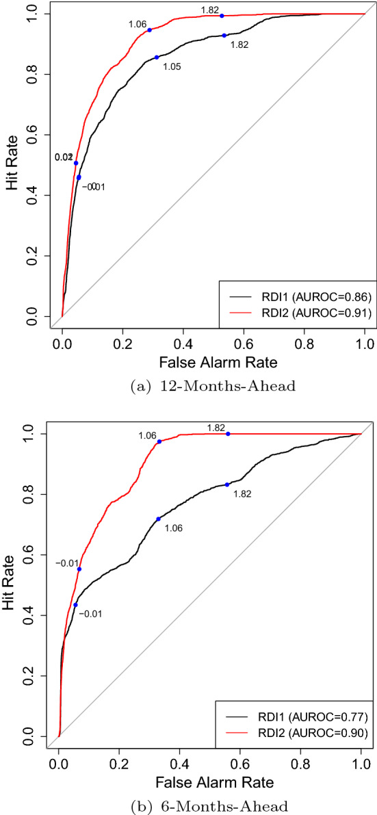
ROC curves of the two RDIs. Note The blue dots mark particular thresholds with their values on the ROC curves. (Color figure online)

Consistent with many previous studies [(e.g., Ng (2012) and Hwang (2019)], the spread worked the best at the 12-horizon in explaining the RDIs, and as a result, we pay special attention to this horizon. In addition, we also experimented with other horizons to explore how forecast horizons and the implied explanatory power of the indicator affect the performance of the RDIs. In Fig. 3, we have plotted the out-of-sample recursively estimated recession probabilities over 1979–2021 associated with the two RDIs based on a static probit model with spread as the only explanatory variable.9 From 12-month-ahead forecasts, we find like (Lai and Ng 2020), RDI2 reflects more probabilities of recessions than RDI1 most of the times. However, with 6-month horizon, surprisingly we do not find the same result. Except for the period 1975–1984, the predicted probabilities for 6-month-ahead forecasts with RDI1 are consistently higher that those with RDI2. Of course, these higher probabilities do not necessarily translate into superior predictions in terms ROC. The AUROC for each horizon and each RDI are reported in Table 3. We see that the AUROC of RDI2 stays high and does not vary much with forecast horizon and is consistently higher than that of RDI1. Note that AUROC of RDI1 is particularly low at horizon 6 (only 0.77), which is not the best horizon of the spread. Even at this horizon, AUROC is 0.90 for RDI2—a gain of nearly 16.9% over RDI1. This highlights the flexibility and robustness of RDI2 over horizons. The result is noteworthy because 6-month is a popular and commonly used horizon in recession forecasting, cf. Stock and Watson (1993b). The composite leading index originally designed by NBER was designed to forecast recessions, like RDI2, more flexibly in the near future (6–9 months), without specifying a specific horizon (see (Lahiri and Moore 1992)). In his comment, Zarnowitz (1993) raised the issue of six-month fixed-horizon forecasting scheme adopted by Stock and Watson (1993a) as a basic departure from the NBER tradition and recommended further research.

Fig. 3.

Out-of-Sample recession probabilities by RDI Note The green lines are for RDI1 and the red lines are for RDI2. (Color figure online)

Table 3.

AUROC comparison by horizon

Horizon	AUROC (RDI1)	AUROC (RDI2)
6	0.77	0.90
9	0.84	0.92
12	0.86	0.91
16	0.84	0.89

Since AUROC is a global measure integrated over all possible (but often not all relevant) threshold values, we also compare the two RDIs by looking at Kuipers score (KS).10 KS for RDI k is defined as

$$\begin{array}{c}\hfill {\text{KS}}^{(k)}(\delta )=H^{(k)}(\delta )-F^{(k)}(\delta ),\end{array}$$ 5

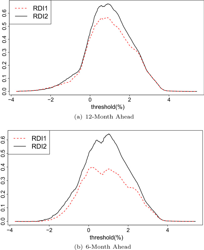
which varies with threshold $\delta$. We plot KS of the two RDIs in Fig. 4 using the whole sample. Berge and Jordà (2011) justifies the Kuiper’s score in terms of a utility function where the benefits of hits equal the costs of misses in absolute value and chose the threshold that maximizes such a function. We find the KS for RDI2 is almost always higher than the KS for RDI1 except a few extreme thresholds, and this wedge is substantially more with 6-month-ahead forecasts, as we found before. The higher RDI1 probabilities for 6-month predictions in Fig. 3 have translated into worse KS values. It can be noted that KS is maximized around threshold values 0.9% to 1% (they are also called Youden’s index). We will pick 0.9% to produce some of the results that we will show later. The conventional threshold value of zero (i.e., inversion of yield spread) would yield considerably lower KS scores. To confirm these results, Fig. 5 shows conditional densities for both RDI1 and RDI2 [$Pr(x|y^{(k)}=1)$ and $Pr(x|y^{(k)}=0)$] at different values of the threshold. The point at which the two densities cross, which is about 0.9%, maximizes KS over the whole sample. Interestingly, the top panels of Fig. 5 indicate that for the first four recessions with both horizons, the KS-maximizing threshold was close to zero (about 0.2%), which is the conventional inversion of the spread. See (Lahiri and Yang 2013) for further elaboration on this result.

Fig. 4.

Kuipers score by threshold

Fig. 5.

Conditional densities. Note Red density curves are conditional on $y^{(k)}=1$. Black dashed density curves are conditional on $y^{(k)}=0$. Densities are based on 12-month-ahead horizon. (Color figure online)

To summarize, when we compare the two RDI’s over the whole sample from 1962-2021 covering all 8 recessions, we find overwhelming evidence that the same predictor will look more successful using RDI2 as the forecast object derived from the NBER recession chronologies. In this sense, RDI2 will make the forecasts look more successful than RDI1 in predicting the same sequence of recessions. Lai and Ng (2020) have argued that RDI2 is also more appropriate from the standpoint of policy maker. However, it is conceivable that RDI1 may be more appropriate in a different policy environment, e.g., knowing the exact timing of a stock market crash may be useful to avoid selling stocks in a bull market too early. For different practitioners, the usefulness and reliability of each RDI vary, given the same sequence of recessionary signals. For forecast users who care less about the exact timing of the regime change, RDI2 may be a better choice.

Comparison of the two RDIs for individual recessions

To gain further insights into factors that are giving the edge to RDI2 over RDI1, we examine their relative performance episodically covering 8 recessions since 1969 one by one. These recessions spanned (1969:12–1970:11), (1973:11–1975:3), (1980:1–1980:7), (1981:7–1982:11), (1990:7–1991:3), (2001:3–2001:11), (2007:12–2009:6) and (2020:2–2020:4). Since they have been highly heterogeneous in terms of duration, predictability and sharpness, we can possibly tease out the independent contributions of differing forecasts and contexts on their relative performance. For instance, over the sample the duration of recessions varied from 2 to 18 months. Except for the recessions of 1981:7–1982:11 and 2007:12–2009:3, the other recessions in our sample were followed by months of growth slowdowns and hence were possibly more predictable, see Lahiri (2010).

We start the recession-by-recession evaluation two years before the beginning of each recession and end at the last day of the recession. For the (1981:7–1982:11) recession, we start from one year before since there is only one year between the end of 1980 recession and the beginning of 1981 recession. The threshold is fixed at $\delta =0.9\%$ for latest four recessions, which is the threshold that yields best overall KS as already shown. For the first four recessions in our sample, the threshold is set at $\delta =0.2\%$ since our experiments showed a value around 0.2 was optimal in earlier decades. We consider both 6-month and 12-month horizons to find their independent effects. Table 4 reports the forecast evaluations recession by recession. The most immediate observation is that for the recessions of 1973:11–1975:3 (recession 2) and 1990:7–1991:3 (recession 5) with horizon 12 forecasts, RDI1 performed better that RDI2 in terms of higher hit rate, lower false alarm rate and consequently higher Kuiper’s score. But for horizon 6, RDI1 lost the edge for recession 5 (i.e., 1990:7–1991:3), but continued to maintain its superiority for recession 2 (i.e., 1973:11–1975:3). In all other cases in Table 4, RDI2 yields superior performance. In order to appreciate the role of the length of recessions, and the behavior of the spread before and during recession, we have presented the plots of yield spread together with the values of RDI1 and RDI2 for each recession for the two horizons separately in Figs. 6 and 7. In these graphs, the red (dotted) and blue lines represent periods in which $y_t^{(1)}=1$ and $y_t^{(2)}=1$, respectively. $y_t^{(1)}=0$ in periods without red dotted line and $y_t^{(2)}=0$ in periods without blue line. The lines are plotted at KS-maximizing thresholds of the spread. A recession is signaled or not signaled if the spread is below or above the level these two horizontal lines mark.

Table 4.

Forecast outcomes by recession

	H (RDI1)	H (RDI2)	F (RDI1)	F (RDI2)	KS(RDI1)	KS(RDI2)
12-month-ahead
Recession 1	0.75	0.77	0.26	0.23	0.49	0.54
Recession 2	0.64	0.52	0.26	0.36	0.39	0.16
Recession 3	1.00	1.00	0.48	0.31	0.52	0.69
Recession 4	0.65	0.76	0.01	0.09	0.64	0.67
Recession 5	1.00	0.85	0.37	0.33	0.63	0.52
Recession 6	1.00	1.00	0.26	0.11	0.74	0.89
Recession 7	0.60	0.86	0.50	0.42	0.10	0.43
Recession 8	1.00	1.00	0.74	0.55	0.26	0.45
6-month-ahead
Recession 1	0.67	0.92	0.29	0.31	0.38	0.61
Recession 2	0.93	1.00	0.07	0.31	0.86	0.69
Recession 3	1.00	1.00	0.48	0.48	0.52	0.52
Recession 4	0.43	0.89	0.31	0.23	0.12	0.66
Recession 5	0.52	0.70	0.53	0.49	0.00	0.21
Recession 6	0.77	1.00	0.33	0.31	0.43	0.69
Recession 7	0.27	0.71	0.75	0.52	−0.48	0.20
Recession 8	1.00	1.00	0.74	0.68	0.26	0.32

The recessions spanned (1969:12–1970:11), (1973:11–1975:3), (1980:1–1980:7),(1981:7–1982:11), (1990:7–1991:3),(2001:3–2001:11),(2007:12–2009:6) and (2020:2–2020:4). For recession samples 1–3 and 5–8, each sample is from 2 years before the recession began to the end of it. Recession 4 (1981 recession) is from 1 year before the recession began to the end of it. The threshold is $\delta =0.2\%$ for the first 4 recessions and $\delta =0.9\%$ for the last 4 recessions

H is hit rate, F is false alarm rate and KS is Kuipers score

Fig. 6.

Two RDIs in each recession: 12-Month-head. Note Black lines represent the spread. Red dotted lines represent periods in which RDI1 is equal to 1. Blue lines represent periods in which RDI2 is equal to 1. The lines of both RDIs are drawn at the value of the threshold we use (0.2% for the first 4 recessions and 0.9% for the last 4 recessions) to help us see whether the spread is below it or not. (Color figure online)

Fig. 7.

Two RDIs in each recession: 6-month-ahead. Note See Fig. 6 for explanations

Recession 1 (1969:12–1970:11): The KS for the two RDIs is similar at 12-month horizon with the KS of RDI2 being a little higher. This is because the duration of this recession was 11 months, which is close to the forecast horizon. Thus the two RDIs overlap most of the time and yield similar results. The slight difference comes from the 1-month-long non-overlapping period, which can be seen in Fig. 6a. When it comes to 6-month horizon, RDI2 has better KS. The explanation is endorsed by Fig. 7a, where we see a period in which $y_t^{(1)}=1$ and $y_t^{(2)}=0$ at the beginning of the recession, which is related to the fact that the forecast horizon is shorter than recession duration. The value of the spread went up high early at the beginning of that recession, giving non-recessionary signals, which are counted as false by RDI1, lowering the hit rate. The hit rate of RDI2, on the other hand, is not affected since there are no more peak turning points when forecasts are made inside the recession.

Recession 2 (1973:11–1975:3): At the 12-month horizon, quite remarkably KS for RDI1 is 0.39 which is higher than 0.16, the KS of RDI2. The explanation is related to the extra false alarms by RDI2 inside the long recession. The value of the spread continued to be low and negative during this recession, giving continued recessionary forecasts, which are counted as false by RDI2 and true by RDI1. As a result, the false alarm rate for RDI1 is lower than that of RDI2. This is a case in which RDI1 "benefits" from the long duration of a recession, and the fact that the predictor continued to signal recessions after the onset. The explanation above can be confirmed in Fig. 6b, where $y_t^{(1)}=1$, $y_t^{(2)}=0$ and ${\widehat{y}}_t=1$ (spread being below the threshold) in the first few months of the recession. By comparison, the results at 6-month horizon are very close and similar explanations follow (see Fig. 7b).

Recession 3 (1980:1–1980:7): At the 12-month horizon, the KS for RDI2 is higher at 0.69 due to lower false alarm rate. The duration of the 1980 recession is relatively short (6 months). In Fig. 7c, the recessionary forecasts 6 months before the beginning of the recession are counted as true by RDI2 since RDI2 is not sensitive in terms of timing. But these recessionary forecasts are counted as false alarms by RDI1, because although the recession started soon, it ended so early that it no longer existed 12 months later. At the 6-month horizon, the results for the two RDIs are same since the duration of the recession is same as the forecast horizon, and the two RDIs overlap.

Recession 4 (1981:7–1982:11): At the 12-month horizon, the KS for the two RDIs is similar at 0.64 and 0.67. This is because during the non-overlapping period at the beginning of the recession, the extra false alarms and extra true negative forecasts by RDI2 offset each other; see Fig. 6d. At the 6-month horizon, KS of RDI1 becomes much lower due to a lower hit rate. The duration of this recession is 16 months, which is 10 months longer than the forecast horizon. The spread was high most of the time during the recession, giving non-recessionary forecasts that are counted as false by RDI1 and true by RDI2 during the first 10 months of the recession (see Fig. 7d). This produced a low hit rate for RDI1. It is an example in which RDI2 "benefits" from its less sensitivity to recession duration: once the recession started, RDI2 assumed 0 values and there was no more concern for lower hit rates.

Recession 5 (1990:7–1991:3): At the 12-month horizon, the KS for RDI1 is 0.63 which in higher than 0.52, the KS for RDI2. In Fig. 6e, there is a period before the recession in which $y_t^{(1)}=0$ and $y_t^{(2)}=1$. The value of the spread went up significantly during this period and gave non-recessionary signals, which are false by RDI2. These non-recessionary forecasts are counted as true by RDI1 since the recession ended early. Thus the hit rate for RDI1 is higher than the hit rate for RDI2. This is an example in which RDI1 "benefits" from the short duration of a recession and early recovery of the predictor, which can be important to many people in finance who care about timing. At 6-month horizon, RDI1 no longer yields better-looking results due to its lower hit rate. The explanation is similar to that of recession 4 (6-month-ahead); see Fig. 7e.

Recession 6 (2001:3–2001:11): The results for RDI2 are better for both horizons. For this short recession that lased just for 8 months, RDI2 benefits again from its less stringency at horizon 12, as has been true for recession 3. Also, since the recession duration is longer than 6 months, RDI1 has about additional 2 months of false negatives (missing recession) during the first two months of the recession that lowered its hit rate.

Recession 7 (2007:12–2009:6): Recession 7 is another long recession. RDI2 yields better-looking results for both horizons, again due to its less sensitivity to recession duration. The explanation is similar to that of recession 4 (1981:7–1982:11). Even though this recession is long like recession 2 (1973:11–1975:3), the behavior of spread before and during the recession was quite different. The high false alarm rates of both RDIs are due to an early drop of the spread before 2006, whose recessionary signals were correct economically, but too early to be counted as true by both RDIs. Borio et al. (2020) had an insightful discussion on this issue.

Recession 8 (2020:2–2020:4): Recession of 2020 is very short due to the special circumstances associated with COVID-19. RDI2 yielded better-looking results for both horizons due to its less stringency. The reasons are similar to that of recessions 6 and 3. However, the extraordinary elevated false alarm rates are caused again by an early drop of the spread, as seen in Fig. 7h.

One message that comes out clearly from the above analysis is that time profile of recessionary signals before and during the recession has to synchronize with onset and duration of the recession to maximize the discriminatory power of a RDI. Often, the spread as the sole predictor inverts for few periods and recovers quickly. In these cases, both RDIs will generate many false signals if the recession turns out to be long. Recent work by Lai and Ng (2020) and Borio et al. (2020) suggests that if spread is supplemented with other relevant recession predictors with predictive value at alternative forecast horizons, the composite predictor can possibly increase the hit rate without sacrificing on the false alarm rate.

In recent years, a number of important papers have explored the role of different types of yield spreads and other predictors in forecasting recessions in the Eurozone and other areas often using AUROC (see Moneta (2005), Bellégo and Ferrara (2009), Fendel et al. (2021) and Sabes and Sahuc (2022)). The methodology developed in this paper can be applied to other countries as well. Finally, we should point out that our results are normative and can not be used ex ante to choose one RDI or the other. It should be dictated by the expectation regarding the onset date and duration of the next recession and loss function of the forecaster in a particular decision-making context.

A third RDI

Peláez (2015) has introduced the so-called semiannual recession forecasting model where instead of forecasting the months or starting months of recessions, it forecasts the half-year of the turn. Thus, his forecast object is defined to be equal to 1 for the periods starting from the calendar half-year containing an NBER peak month to the calendar half-year containing the next trough month and 0 for other periods. Thus Peláez converted the NBER recession dummy to a biannual chronology. As long as there is at least one month in a half-year being an NBER recession, the whole half-year becomes recession. For example, the 2001:3–2001:11 recession (our recession 6) spanned first half and second half of 2001 in Peláez’s re-definition, lasting for 12 months.

With semiannual observations, Peláez showed that his simple forecasting model with yield spread and a composite financial variable successfully predicted all peaks since the 1970s without any false positives. It also outperformed (Wright 2006)’s specification. Even though (Peláez 2015) did not propose his bi-annual model as another RDI, we have pointed out before that it can indeed be interpreted another RDI. As a natural extension to our analysis, we now consider his re-definition and compare with RDI1 and RDI2.

Note that in order to evaluate his semiannual chronology as another RDI, it is not necessary to convert all the data to semiannual averages. Thus, for the purpose of comparability, we make the frequency of this definition daily, but keep the dates of peaks and troughs same as Peláez’s RDI3. Following Peláez’s idea, the 2020 recession (recession 8) in this definition is from the first day of January to the last day of June 2020. The dates of other recessions are defined in the fourth and fifth columns of Table 1 in Peláez (2015). We call this RDI3, which is defined as

$$\begin{array}{c}\hfill y_t^{(3)}=I_{t+h}^{(s)},\end{array}$$ 6

where $I_{t+h}^{(s)}$ is a semiannual chronology (turned into daily in our analysis) of recession indicator by Peláez. We computed all the forecast evaluation statistics for RDI3. The ROC curves of RDI3 are plotted against the other two RDIs in Fig. 8 in the top panel. The H, F and KS of RDI3 are reported in Table 5. It can be seen that the results of RDI3 are in-between the results of the other RDIs in terms of hit rates, false alarm rates and AUROC. Since RDI3 tends to make the forecast object wider, it is presumably easier to hit. For instance, the average length of recessions in the Peláez RDI is 16.2 months compared with 12.2 months in the original NBER chronologies. As we see in these tables, RDI3 gives results that are close to RDI1, but considerably less discriminatory than RDI2. Our approach evaluates Peláez’s proposal as a new RDI, but without making the empirical implementation using bi-annual observations. By implication, the extraordinary favorable results of RDI3 that (Peláez 2015) reported could have been due to the aggregation of the monthly data to bi-annual averages and making the date of peaks as six-monthly event rather than daily or monthly.

Fig. 8.

ROC curve comparison: 3 RDIs

Table 5.

Forecast outcomes by recession: RDI3

Recession	H	F	KS
	(RDI3)	(RDI3)	(RDI3)
12-month-ahead
Recession 1	0.63	0.18	0.45
Recession 2	0.55	0.20	0.34
Recession 3	0.92	0.33	0.59
Recession 4	0.61	0.01	0.60
Recession 5	0.88	0.31	0.57
Recession 6	0.86	0.19	0.67
Recession 7	0.70	0.34	0.37
Recession 8	1.00	0.68	0.32
6-month-ahead
Recession 1	0.62	0.20	0.42
Recession 2	0.68	0.00	0.68
Recession 3	0.83	0.43	0.40
Recession 4	0.43	0.27	0.17
Recession 5	0.43	0.58	-0.15
Recession 6	0.76	0.25	0.51
Recession 7	0.45	0.67	-0.21
Recession 8	1.00	0.68	0.32

The recessions spanned (1969:12–1970:11), (1973:11–1975:3), (1980:1–1980:7), (1981:7–1982:11), (1990:7–1991:3), (2001:3–2001:11), (2007:12–2009:6) and (2020:2–2020:4). For recession samples 1–3 and 5–8, each sample is from 2 years before the recession began to the end of it. Recession 4 (1981 recession) is from 1 year before the recession began to the end of it. The threshold is $\delta =0.2\%$ for the first 4 recessions and $\delta =0.9\%$ for the last 4 recessions. RDI3 is the definition by Peláez

H is hit rate, F is false alarm rate and KS is Kuipers score

Finally, since most recent studies in this area have used monthly data [(e.g., Stekler and Ye (2017), Lai and Ng (2020) and Vrontos et al. (2021)], we re-generated the results in Fig. 8a, b with monthly data and reported in Fig. 8c, d. We find that the performance and ordering of the three RDIs are remarkably similar, and hence we can conclude that the results reported in this paper are not artifacts of using daily data.11 However, due to the use of more observations in Fig. 8a, b, these curves are smoother that those in Fig. 8c, d. Earlier we have underscored other important advantages of using daily data in our context.

Conclusion

Using yield spread as an illustrative recession predictor and without estimating any parametric model, we formally and quantitatively compare the two alternative recession-derivative indicators that have been used extensively in recession prediction, viz. (1) the target variable takes value 1 if there is an NBER recession exactly at a pre-specified horizon in the future (RDI1); and (2) the target variable takes value 1 if there is a recession that starts any time during the next specified number of periods (RDI2). The model-free approach directly generates forecasts from raw yield spread data, which does not suffer from parameter estimation issues due to model misspecifications and the delayed announcements of turning points by NBER. The ability of the practitioners to monitor the actual values of the yield spread rather than probabilities estimated from an underlying model, and when it gets close to being negative is a real advantage of our approach.

Summarizing our findings, we find that in general RDI2 tends to show better results than RDI1 due to its less demanding definition regarding exactly when the recession will start, and being less sensitive to the length of recessions. However, given the same predictor and the same recession chronology, RDI2 may not yield more favorable results in all circumstances. We identified the following scenarios where RDI1 is expected to produce better-looking results: (1) Recession is short relative to forecast horizon, the predictor falls below the threshold and increases back early before the recession begins and (2) recession is long relative to the forecast horizon, spread does not increase back too early and stays low while inside the recession. With a sample of eight recessions and two forecast horizons, we found three cases where RDI1 has better Kuiper’s score than RDI2, and two other cases where they are very close. Thus, contrary to conventional thinking, the target variable RDI1 that predicts the occurrence of a recession at a specific future date is not always more restrictive than RDI2 that captures the occurrence of a recession within a given future time period. Also, from the standpoint of practitioners like bankers, fund managers and stock traders who track their business on a daily basis and care about the duration and precise timing of a recession, RDI1 can be more relevant than RDI2 for better investment decisions.

We also considered a semiannual RDI proposed by Peláez (2015), but without aggregating the data into biannual, and found that this RDI can produce results better than RDI1, but not as good as RDI2. Note that our conclusions can be generalized with additional predictors and monthly data.

A comprehensive but considerably more demanding RDI should predict the timing of peaks and troughs simultaneously. Lacking this, the intuition we get from our analysis comparing the widely used RDIs is that the relative advantage of a particular RDI depends on forecast horizon, recession duration and the time profile of recession signals before and during the recession. Since these factors are seldom known in real time, the choice of RDI by practitioners should depend on their prior expectation of the peak onset date and the duration of a forthcoming recession at a desired horizon.

Declarations

Conflict of interest

The authors have no conflict of interest to declare that are relevant to the content of this article.

Ethical approval

This article does not contain any studies with human participants or animals performed by any of the authors.

References

- Ajello A, Benzoni L, Schwinn M, Timmer Y, Vazquez-Grande F (2022) Monetary policy, inflation outlook, and recession probabilities. In: FEDS notes. Board of Governors of the Federal Reserve System, Washington. 10.17016/2380-7172.3175
- Bauer MD, Mertens TM. Information in the yield curve about future recessions. FRBSF Econom Lett. 2018;20:1–5. [Google Scholar]
- Bellégo C, Ferrara L (2009) Forecasting euro area recessions using time-varying binary response models for financial variables. Banque de France
- Berge TJ, Jordà Ò. Evaluating the classification of economic activity into recessions and expansions. Am Econom J Macroecon. 2011;3(2):246–277. doi: 10.1257/mac.3.2.246. [DOI] [Google Scholar]
- Bismans F, Majetti R. Forecasting recessions using financial variables: the French case. Empir Econ. 2013;44(2):419–433. doi: 10.1007/s00181-012-0550-z. [DOI] [Google Scholar]
- Borio C, Drehmann M, Xia FD. Forecasting recessions: the importance of the financial cycle. J Macroecon. 2020;66:103258. doi: 10.1016/j.jmacro.2020.103258. [DOI] [Google Scholar]
- Bussiere M, Fratzscher M. Towards a new early warning system of financial crises. J Int Money Financ. 2006;25(6):953–973. doi: 10.1016/j.jimonfin.2006.07.007. [DOI] [Google Scholar]
- Chen YT. A mixed-frequency smooth measure for business conditions. Empir Econ. 2021;61(4):1699–1724. doi: 10.1007/s00181-020-01937-w. [DOI] [Google Scholar]
- Cooper D, Fuhrer JC, Olivei G (2020) Predicting recessions using the yield curve: the role of the stance of monetary policy. Available at SSRN 3587629
- DeLong ER, DeLong DM, Clarke-Pearson DL. Comparing the areas under two or more correlated receiver operating characteristic curves: a nonparametric approach. Biometrics. 1988;44(3):837–845. doi: 10.2307/2531595. [DOI] [PubMed] [Google Scholar]
- Diebold FX (2006) Elements of forecasting. South-Western College Publishing
- Duarte A, Venetis IA, Paya I. Predicting real growth and the probability of recession in the Euro area using the yield spread. Int J Forecast. 2005;21(2):261–277. doi: 10.1016/j.ijforecast.2004.09.008. [DOI] [Google Scholar]
- Ergungor OE (2016) Recession probabilities. Federal Reserve Bank of Cleveland, Economic Commentary 2016-09. 10.26509/frbc-ec-201609
- Estrella A, Mishkin FS. The yield curve as a predictor of U.S. recessions. Curr Issues Econ Financ. 1996;2(7):1–6. [Google Scholar]
- Fendel R, Mai N, Mohr O. Recession probabilities for the eurozone at the zero lower bound: challenges to the term spread and rise of alternatives. J Forecast. 2021;40(6):1000–1026. doi: 10.1002/for.2751. [DOI] [Google Scholar]
- Galán JE, Mencía J. Model-based indicators for the identification of cyclical systemic risk. Empir Econ. 2021;61(6):3179–3211. doi: 10.1007/s00181-020-01993-2. [DOI] [Google Scholar]
- Ghysels E (2013) Matlab toolbox for mixed sampling frequency data analysis using MIDAS regression models. Available on MATLAB Central at http://www.mathworks.com/matlabcentral/fileexchange/45150-midas-regression
- Ghysels E, Hill JB, Motegi K. Testing a large set of zero restrictions in regression models, with an application to mixed frequency Granger causality. J Econ. 2020;218(2):633–654. doi: 10.1016/j.jeconom.2020.04.032. [DOI] [Google Scholar]
- Harding D, Pagan A (2016) The econometric analysis of recurrent events in macroeconomics and finance. Princeton University Press
- Harding D, Pagan AR (2010) Can we predict recessions? NCER Working Paper Series. Working Paper No. 69
- Hsu YC, Lieli RP (2021) Inference for ROC curves based on estimated predictive indices. arXiv preprint arXiv:2112.01772
- Hwang Y. Forecasting recessions with time-varying models. J Macroecon. 2019;62:103153. doi: 10.1016/j.jmacro.2019.103153. [DOI] [Google Scholar]
- Johansson P, Meldrum AC (2018) Predicting recession probabilities using the slope of the yield curve. In: FEDS Notes. Board of Governors of the Federal Reserve System, Washington
- Kaminsky GL, Reinhart CM. The twin crises: the causes of banking and balance-of-payments problems. Am Econ Rev. 1999;89(3):473–500. doi: 10.1257/aer.89.3.473. [DOI] [Google Scholar]
- Krzanowski WJ, Hand DJ (2009) ROC curves for continuous data. CRC Press
- Lahiri K (2010) Transportation indicators and business cycles, contributions to economic analysis, vol 289. Emerald Group Publishing
- Lahiri K, Wang JG. Evaluating probability forecasts for GDP declines using alternative methodologies. Int J Forecast. 2013;29(1):175–190. doi: 10.1016/j.ijforecast.2012.07.004. [DOI] [Google Scholar]
- Lahiri K, Yang L. A further analysis of the conference board’s new Leading Economic Index. Int J Forecast. 2015;31(2):446–453. doi: 10.1016/j.ijforecast.2014.12.006. [DOI] [Google Scholar]
- Lahiri K, Moore GH (1992) Leading economic indicators: new approaches and forecasting records. Cambridge University Press
- Lahiri K, Yang L (2013) Forecasting binary outcomes, handbook of economic forecasting, vol 2. Elsevier, pp 1025–1106
- Lai H, Ng EC. On business cycle forecasting. Front Bus Res China. 2020;14(1):1–26. doi: 10.1186/s11782-020-00085-3. [DOI] [Google Scholar]
- Miller DS (2019) There is no single best predictor of recessions. In: FEDS notes. Board of Governors of the Federal Reserve System, Washington 10.17016/2380-7172.2367
- Moneta F. Does the yield spread predict recessions in the Euro area? Int Financ. 2005;8(2):263–301. doi: 10.1111/j.1468-2362.2005.00159.x. [DOI] [Google Scholar]
- Ng EC. Forecasting US recessions with various risk factors and dynamic probit models. J Macroecon. 2012;34(1):112–125. doi: 10.1016/j.jmacro.2011.11.001. [DOI] [Google Scholar]
- Pagan A (2019) Business cycle issues: some reflection on a literature. Papeles de Economıa Espanola forthcoming
- Peláez RF. A biannual recession-forecasting model. J Macroecon. 2015;45:384–393. doi: 10.1016/j.jmacro.2015.07.002. [DOI] [Google Scholar]
- Sabes D, Sahuc JG (2022) Do yield curve inversions predict recessions in the Euro Area? Financ Res Lett, Forthcoming
- Stekler HO, Ye T. Evaluating a leading indicator: an application–the term spread. Empir Econ. 2017;53(1):183–194. doi: 10.1007/s00181-016-1200-7. [DOI] [Google Scholar]
- Stock, JH, Watson MW (1993a) A procedure for predicting recessions with leading indicators: econometric issues and recent experience. In: Stock JH, Watson MW (eds) New research on business cycles, indicators and forecasting. University of Chicago Press
- Stock, JH, Watson MW (1993b) Introduction to “business cycles, indicators and forecasting”. In: Stock JH, Watson MW (eds) New research on business cycles, indicators and forecasting. University of Chicago Press
- Vrontos SD, Galakis J, Vrontos ID. Modeling and predicting us recessions using machine learning techniques. Int J Forecast. 2021;37(2):647–671. doi: 10.1016/j.ijforecast.2020.08.005. [DOI] [Google Scholar]
- Wright JH (2006) The yield curve and predicting recessions. Finance and Economics Discussion Series 2006-07, Federal Reserve Board
- Yang L, Lahiri K, Pagan A (2022) Getting the ROC into Sync. Forthcoming in J Bus Econ Stat
- Zarnowitz V (1993) Comment on stock and Watson. In: Stock JH, Watson MW (eds) New research on business cycles, indicators and forecasting. University of Chicago Press