Robust state estimation of feeding–blending systems in continuous pharmaceutical manufacturing

Abstract

State estimation is a fundamental part of monitoring, control, and real-time optimization in continuous pharmaceutical manufacturing. For nonlinear dynamic systems with hard constraints, moving horizon estimation (MHE) can estimate the current state by solving a well-defined optimization problem where process complexities are explicitly considered as constraints. Traditional MHE techniques assume random measurement noise governed by some normal distributions. However, state estimates can be unreliable if noise is not normally distributed or measurements are contaminated with gross or systematic errors. To improve the accuracy and robustness of state estimation, we incorporate robust estimators within the standard MHE skeleton, leading to an extended MHE framework. The proposed MHE approach is implemented on two pharmaceutical continuous feeding–blending system (FBS) configurations which include loss-in-weight (LIW) feeders and continuous blenders. Numerical results show that our MHE approach is robust to gross errors and can provide reliable state estimates when measurements are contaminated with outliers and drifts. Moreover, the efficient solution of the MHE realized in this work, suggests feasible application of on-line state estimation on more complex continuous pharmaceutical processes.

1. Introduction

Development and application of advanced monitoring, control, and decision-making strategies for continuous pharmaceutical manufacturing require a good understanding of the current state of the system. However, obtaining accurate description of the state in real time can be very challenging due to several theoretical or practical complexities. First, it is impossible to directly measure all of the state variables that are related to the product quality attributes. In addition, many state variables cannot be measured in real time, leading to time delays longer than the dynamic response of the process. As a result, some critical state variables, if not directly or instantly measured, must be estimated from available measurements. Moreover, measurements are subject to random errors which may arise from uncertainties in the process, change in ambient environment, and signal noise during transmission and conversion. To reduce undesirable effects caused by random noise, it is also necessary to reconcile the measured values. Therefore, real-time state estimation plays a crucial role in efficient monitoring and control of product quality attributes in continuous pharmaceutical manufacturing processes.

Given sufficient measurements, one can estimate the current state from a mathematical model which, either first-principles or data-driven, describes the relationships between the measured and unmeasured states. Additionally, state estimation usually considers measurement noise and/or process disturbances. The classical Kalman filter (KF) is an optimal state estimator designed for unconstrained, linear systems with random noise governed by some normal distribution. However, it is not directly applicable in many real-world physical systems with hard constraints and nonlinear properties. As a result, a large body of KF-based extensions have been proposed, such as the extended Kalman filter (EKF) (Bryson, 1975), the unscented Kalman filter (UKF) (Julier et al., 2000), and the ensemble Kalman filter (Houtekamer and Mitchell, 1998). Other related state estimation techniques include the particle filtering (PF) (Arulampalam et al., 2002), nonlinear recursive dynamic data reconciliation (Vachhani et al., 2005, 2006) and multiple model (MM) approaches (Arulmaran and Liu, 2017).

On the other hand, moving horizon estimation (MHE) provides an alternative approach to estimate the state of the system, which uses a set of past measurements within a receding time horizon. The current state is estimated by solving an optimization problem which explicitly considers nonlinear system dynamics, multivariate relationships between state variables, and hard constraints arising from physical and/or operational limits. MHE is usually formulated as a dynamic optimization (DO) problem constrained by a set of differential algebraic equations (DAEs). Previous studies have shown that nonlinear, constrained MHE has desirable stability properties (Rao et al., 2003) and often outperforms the EKF (Abrol and Edgar, 2011; Haseltine and Rawlings, 2005). However, the high computational burden is the major challenge in real-time application of MHE (Ramlal et al., 2007). Fortunately, advanced computational and solution strategies have made it possible to solve nonlinear MHE problems efficiently (Abrol and Edgar, 2011; Nicholson et al., 2014). In this paper we focus on developing an MHE framework for continuous pharmaceutical processes.

In conventional state estimators, measurement errors are usually assumed to be random and normally distributed. However, this assumption cannot always be validated since the actual distributions of random errors are often unknown. Moreover, traditional state estimators fail to consider gross errors or bias, which are relatively lower-frequency, nonrandom errors commonly caused by improper installation of instruments, incorrect calibration of sensors, or inadequate maintenance. The presence of gross errors can contaminate the reconciled measurements and estimates, causing undesirable “smearing” effects (Ozyurt and Pike, 2004). To improve the accuracy and robustness of estimators, research in state estimation is closely related to topics of data reconciliation (DR) and gross error detection (GED).

Robust estimators, also known as maximum likelihood estimators or M-estimators, are commonly used in reconciling measurements contaminated with gross errors. Tjoa and Biegler (1991) initially proposed a DR problem with the contaminated Normal function. The proposed approach was able to provide unbiased estimates in the presence of gross errors without requiring procedures involving iterative use of statistical tests. Subsequently, Arora and Biegler (2001) presented a data reconciliation and parameter estimation strategy implemented using the Fair function and the Hampel redescending M-estimator. Recently, these robust estimators have been implemented in an on-line state estimation framework and tested in nonlinear dynamic systems such as continuous stirred-tank reactor (CSTR) and distillation column (Nicholson et al., 2014). Other proposed robust estimation techniques use Lorentzian, Logistic, Huber, and Welsch estimators (Albuquerque and Biegler, 1996; Bourouis et al., 1998; Chen et al., 1998; Fuente et al., 2015; Johnston and Kramer, 1995). Systematic comparisons of these various robust estimators can be found in the literature (Ozyurt and Pike, 2004; Prata et al., 2008). Inspired by previous work (Nicholson et al., 2014), we incorporate robust estimators within the standard MHE skeleton, leading to an extended MHE for dynamic state estimation with gross errors.

The proposed MHE technique is implemented and tested on two feeding–blending system (FBS) configurations. In continuous tablet or capsule production lines, the FBS is the last step at which major changes in product composition can be introduced, mitigated, or managed. Beyond this blending step, the product composition is largely fixed since final product or intermediate streams cannot be reworked. As a result, the optimal operation of the FBS is crucial in order to meet the critical quality attributes of the final product. Advanced operation strategies, especially model predictive control (MPC), have been proposed for continuous power blending (Rehrl et al., 2016). However, these techniques require accurate estimates of the current state of the system. To the best of our knowledge, however, little work has been done on the real-time state estimation of a continuous blending process.

The rest of this paper is organized as following. The extended MHE strategy and robust estimators are described in more detail in Section 2. The nonlinear dynamic model of the FBS is provided in Section 3. In Section 4, we compare the standard and extended MHE techniques on simulation runs. Finally, conclusions are provided in Section 5.

2. Moving horizon estimator

In this section, we first introduce the standard moving horizon estimation (MHE) approach. We then incorporate the robust estimators within the classic MHE skeleton, leading to an extended MHE framework which is suitable for nonlinear dynamic systems with gross errors.

2.1. Moving horizon estimation problem

MHE is a well-known strategy for constrained state estimation. The basic idea in MHE is to estimate the current state of the system using only the last L states and measurements directly, where L is the horizon length. In MHE we split time into two sets T_past = {t|0 ≤ t < k − L} and T = {t|k−L ≤ t ≤ k}, where k is the current time. Set T_past includes all time in the past and increases as time goes by. Time in T_past are not considered since the states in the past are not directly impacting the current state. Therefore, in an MHE problem we only consider the time steps in the current time horizon T. The mathematical formulation of a standard MHE problem is given by

$$\begin{array}{c}\text{min\hspace{0.17em}}\Phi (\text{z}(k-L))+\frac{1}{2}\sum _{t\in T_M}{v}^T(t)Q^{-1}(t)v(t)+\frac{1}{2}\sum _{t\in T_M}{w}^T(t)R^{-1}(t)w(t)\\ \begin{array}{lll}\text{s}.\text{t}.\hfill & \text{z}(t)=f(\frac{d\text{z}}{dt},\text{z},p^{*})+v(t)\hfill & \forall t\in T\hfill \\ \hfill & \widehat{x}(t)=h\left(\text{z},p^{*}\right)+w(t)\hfill & \forall t\in T\hfill \\ \hfill & {\text{z}}^L\le \text{z}(t)\le {\text{z}}^U\hfill & \forall t\in T\hfill \end{array}\end{array}$$ (1)

where T_M = {k − L, k − L + 1, … , k − 1, k} is a set of time when state variables are measured, z (t) ∈ ℜ^N is a vector of state estimates at time t, v (t) ∈ ℜ^N is a vector of unknown disturbance, and w (t) ∈ ℜ^M is a vector of measurement errors. Q (t) ∈ ℜ ^N×N is the covariance matrix of the unknown disturbances and R (t) ∈ ℜ^M×M is the covariance matrix of the measurement noise. Matrices Q and R are obtained from previous measurements and regarded as constants in the MHE problem. The arrival cost function Φ(·) presents all the information in the past time horizon T_past. Given a sufficient large horizon length L, the influence from the past is negligible and the arrival cost function Φ(·) can be ignored. In the constraints, f(·) is the system model, h(·) is the measurement model, $\widehat{x}(t)\in {\Re }^M$ is a vector of actual measurements, and p* is a vector of constants. Finally, z^L and z^U indicate lower and upper bounds of the state variables, respectively. In general, the standard MHE is formulated as a dynamic optimization (DO) problem constrained with differential algebraic equations (DAEs).

2.2. Robust estimators

In the standard MHE problem (1), measurement noise is assumed to follow a normal distribution with zero mean and known variance. However, this assumption is violated if the actual distribution of random noise is not normal or available measurements are contaminated with gross errors. In either case, unfortunately, the traditional weighted least squares (WLS) estimators will lead to inaccurate state estimates. Thus we need to introduce new estimators to improve the accuracy and robustness of the MHE.

Robust estimators, also known as the maximum likelihood estimators or M-estimators, are originally proposed for robust statistics. The inherent robustness of these estimators provides a way to handle unknown distributions of random noise and measurements contaminated with gross errors. By replacing the WLS with more generalized maximum likelihood function, the extended MHE problem is given by

$$\begin{array}{c}\text{min\hspace{0.17em}}\Phi (z(k-L))+\frac{1}{2}\sum _{t\in T_M}{v}^T(t)Q^{-1}(t)v(t)+\sum _{t\in T_M}\rho (w(t))\\ \begin{array}{lll}\text{s}.\text{t}.\hfill & \text{z}(t)=f(\frac{dz}{dt},\text{z},p^{*})+v(t)\hfill & \forall t\in T\hfill \\ \hfill & \widehat{x}(t)=h\left(\text{z},p^{*}\right)+w(t)\hfill & \forall t\in T\hfill \\ \hfill & {\text{z}}^L\le \text{z}(t)\le {\text{z}}^U\hfill & \forall t\in T\hfill \end{array}\end{array}$$ (2)

where ρ_t(·) can be any reasonable monotonic function. To concentrate our focus on the measurement errors w(t), in the rest of this paper, we ignore the arrival cost function Φ(·) and assume that the unknown disturbances v(t) are still normally distributed.

A variety of robust estimators have been used in data reconciliation (DR) and gross error detection (GED) (Arora and Biegler, 2001; Chen et al., 1998; Johnston and Kramer, 1995; Tjoa and Biegler, 1991). Ozyurt and Pike (2004) first presented a comparative analysis among six different estimators. The numerical results show that the Cauchy distribution and the Hampel redescending M-estimator outperform over other alternatives in terms of solution quality and computational efficiency. Subsequently, Prata et al. (2008) extended previous work by comparing robust estimators on nonlinear dynamic data reconciliation (NDDR) in the presence of gross errors. The comparison indicates that the Lorenzian and Welsch estimators are more attractive. Recently, Llanos et al. (2015) proposed two estimation frameworks based on the biweight function and compared them with three robust estimators. The numerical results reported show no clear superiority of one M-estimator over the others on all of their test cases. In this paper we consider four robust estimators, whose gross features are shown in Fig. 1a. The first derivative of each robust estimator, also known as the influence function, shown in Fig. 1b, is useful in describing the penalty or weight which is contributed by the errors.

Fig. 1 –

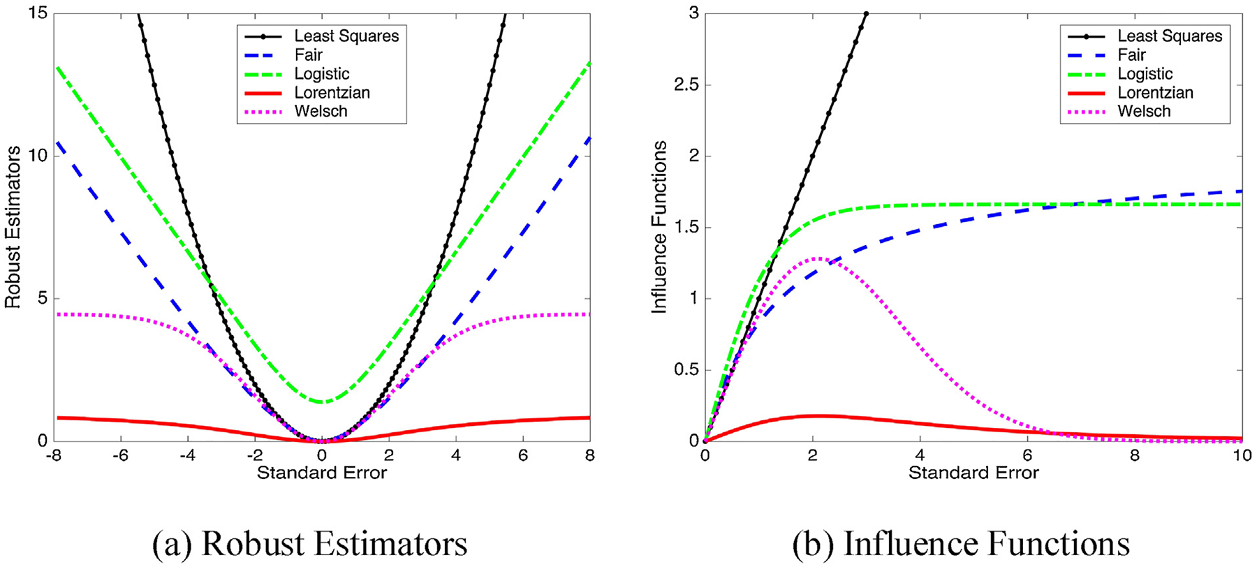
Robust estimators and influence functions.

The Fair function (Fair, 1974) is widely-used in robust data reconciliation

$${\rho }_F(\epsilon )=2c_F^2\left[\frac{\left|\epsilon \right|}{c_F}-\text{ln}\left(1+\frac{\left|\epsilon \right|}{c_F}\right)\right]$$ (3)

where c_F is a tuning parameter and ε = w/σ is the studentized residual. The Fair function is a close approximation of the least squares function for small errors. As the residuals increase, however, the Fair function becomes a linear function of |ε|. In other words, as |ε| approaches infinity, the Fair function put less weight on large errors compared with the least squares function. The shape of the Fair function is determined by the parameter c_F. Smaller values of c_F will cause the Fair function to become linear at smaller errors thus causing it to deviate more from the least squares function.

The Logistic function, given by

$${\rho }_{Lo}(\epsilon )=2\text{ln}\left[1+\text{exp}\left(1+\frac{\left|\epsilon \right|}{c_{Lo}}\right)\right]-\left(\frac{\left|\epsilon \right|}{c_{Lo}}\right)$$ (4)

has a similar shape as the Fair function. However, it does not provide a good approximation of the least squares function for small errors. Note that their influence functions increase monotonically and asymptotically approach some positive values as |ε| approaches infinity. Thus the Fair and Logistic functions are categorized as convex estimators in this work.

The Welsch estimator was introduced by Dennis and Welsch (1978)

$${\rho }_{\text{W}}(\epsilon )=\frac{c_{\text{W}}^2}{2}\left\{1-\text{exp}\left[-{\left(\frac{\epsilon }{c_{\text{W}}}\right)}^2\right]\right\}$$ (5)

Unlike the convex estimators, the influence function of the Welsch estimator increases within a relatively small range of |ε|, and then decreases as the error becomes larger. As a result, the nonconvex Welsch function belongs to the group of redescending estimators. The Lorentzian function is a redescending estimator introduced by Johnston and Kramer (1995)

$${\rho }_L(\epsilon )=1-\frac{1}{1+\left({\epsilon }^2/2c_{\text{L}}^2\right)}$$ (6)

Note that the Lorentzian function is not a good approximation of the least squares function. For both redescending M-estimators, the influence functions asymptotically approach zero as the error approaches infinity and no extra penalty will be put on a very large error. Therefore, redescending estimators are in general less sensitive to outliers and gross errors than the convex estimators. However, an MHE formulation with a non-convex redescending M-estimator may converge to inferior local solutions and initialization techniques are necessary to guarantee good solution quality in some cases (Nicholson et al., 2014; Ozyurt and Pike, 2004).

For the purpose of comparison, robust estimators must be carefully tuned to have similar efficiencies. In this work, however, our primary goal is to demonstrate the benefits obtained from using robust estimators in the MHE framework. Moreover, previous work has shown that performance of robust estimators is not sensitive within a range of parameter values (Nicholson et al., 2014). Therefore, systematical tuning of the robust estimators is not required. In this work, the parameters are fixed to the optimal values recommended in the literature (Nicholson et al., 2014; Ozyurt and Pike, 2004; Prata et al., 2008).

3. Dynamic model of feeding–blending systems

In continuous tablet or capsule production lines, the optimal operation of the feeding–blending system is crucial in order to meet the critical quality attributes (CQAs) of the final product. Advanced monitoring and control strategies of a powder blending process require accurate estimation of the current state of the system. To demonstrate our extended MHE framework, we consider the feeding–blending system in the pharmaceutical continuous manufacturing pilot plant at Purdue University, consisting of loss-in-weight screw feeders and continuous blenders. Previous modeling approaches for continuous power mixing process are categorized as Monte-Carlo methods (Marikh et al., 2006), residence time distribution (RTD) approaches (Gao et al., 2011), discrete element method (DEM) models (Dubey et al., 2011), population balance models (PBMs) (Sen and Ramachandran, 2013), and hybrid models combining the DEM and PBM (Sen et al., 2013). However, solving these models usually comes at the cost of long computational time. Moreover, it is challenging to directly integrate these models within the MHE framework. In this section, we focus on developing a reduced-order mathematical model for the FBS in the continuous manufacturing line, including a first-principles dynamic model for screw feeders and a semi-empirical compartment-based model for continuous blenders. The extended MHE problem formulation is given in more detail with the proposed dynamics models as constraints.

3.1. Dynamic model for feeder

Loss-in-weight (LIW) feeders, particularly screw feeders, are widely used in continuous pharmaceutical processes as sources of material input to the systems. The screw-conveying mechanism of LIW feeders is most rigorously described using DEM-based models (Cleary, 2007; Hu et al., 2010; Imole et al., 2016). However, the resulting models are computationally too demanding to be solved within an MHE problem. By contrast, reduced-order models, such as first-order transfer models, are usually used to approximate the dynamics of LIW feeders (Boukouvala et al., 2012; Singh et al., 2013).

In this work, we present a first-principle model of LIW feeders, where the mass flow rate is a function of mass hold-up in the hopper and rotation speed of the screw. The nonlinear dynamic model is given by

$$\begin{gathered} \frac{d{M}_F(t)}{dt}=-F_F(t) \\ {F}_F(t)={\alpha }_F\frac{{\omega }_F(t)}{{\omega }_F^{*}}\left\{1+{\beta }_F\frac{M_F(t)}{M_F^{*}}+{\gamma }_F{\left[\frac{M_F(t)}{M_F^{*}}\right]}^2\right\} \end{gathered}$$ (7)

where M_F is the total mass hold-up in the hopper, F_F is the mass flow rate of the feeder, and ω_F is the rotation speed of the screw. Parameters ${\omega }_F^{*}$ and $M_F^{*}$ are the standard rotation speed and the mass hold-up. In addition, α_F is the proportional parameter, β_F and γ_F are parameters related to the normalized mass hold-up. Note that values of these parameters are determined by the geometry of the feeder, configuration of the screw, and physical properties of the materials. As a result, these parameters must be carefully calibrated using the same materials and under the same normal operating and environment conditions.

3.2. Dynamic model for blender

Continuous blenders are used to mix multiple powders or granular materials into a blend of uniform composition. The performance of a blender is strongly related to the vessel geometry, agitator configuration and agitator rpm. While, as noted earlier, mixing mechanism has been represented using a variety of detailed an computationally demanding models, recently, Rehrl et al. (2016) proposed a “tank-in-series” model, where the blender is separated into N small compartments or tanks. The mass hold-up of each compartment is modeled by mass balance equations and the outlet active pharmaceutical ingredient (API) concentration is modeled based on the RTD approach.

As an extension, we propose a “CSTR-in-series” model, where each compartment is treated as an ideal CSTR. Similar to the “tank-in-series” model, the outlet mass flow rate of each compartment n ∈ {1, …, N} is a function of the current mass hold-up and the blender rpm. In addition, the CSTR model allows us to explicitly consider the key component concentration in each compartment. The proposed “CSTR-in-series” model provides a reduced-order mathematical description of the dynamics of a continuous blender.

The dynamics of the mass hold-up M_B,n in compartment n can be described by

$$\frac{d{M}_{B,n}(t)}{dt}=F_{B,n-1}(t)-F_{B,n}(t)\forall n$$ (8)

where F_B,n is the outlet mass flow of compartment n. Note that F_B,n is also the inlet mass flow of compartment n + 1 for n < N. In particular, F_B,0 and F_B,N are the inlet and outlet mass flow rates of the blender, respectively. We assume that F_B,n depends on the mass hold-up M_B,n and the agitator rotation speed ω_B

$$F_{B,n}(t)={\alpha }_B{\left[\frac{{\omega }_B(t)}{{\omega }_B^{*}}\right]}^{{\beta }_B}{\left[\frac{M_{B,n}(t)}{M_{B,n}^{*}}\right]}^{\gamma B}\forall n$$ (9)

where ${\omega }_B^{*}$ and $M_{B,n}^{*}$ are the rotation speed and the mass hold-up under the normal operating condition, respectively. Both of these variables are treated as given constants in our model. In addition, α_B is the proportional parameter, β_B and γ_B are the exponential parameters related to normalized rotation speed and mass hold-up, respectively. The values of these parameters are related to configurations of the agitator and physical properties of the mixture. Note that the number of compartments N is also a parameter in our model.

It is possible to consider various parameter values for different compartments. For instance, properties of a compartment, such as size and location, can impact the parameter settings. However, inclusion of that may lead to a large number of unknown parameters and the resulting dynamic model may be over-fitted. Thus α_B, β_B, and γ_B are treated as global parameters in our dynamic model, meaning that their values are shared by all compartments.

Another important part is the dynamics of the key component concentration C_B,n. According to the ideal CSTR model, we have

$$\frac{d{C}_{B,n}(t)}{dt}=\frac{F_{B,n-1}(t)}{M_{B,n}(t)}\left[C_{B,n-1}(t)-C_{B,n}(t)\right]\forall n$$ (10)

Similarly, variable C_B,n is also the concentration of the inlet flow of compartment n + 1 for n < N. In particular, C_B,0 and C_B,N are the inlet and outlet key component concentrations of the blender, respectively. Again, all CSTRs are assumed to have identical properties such as compartment volume and mixing uniformity.

To verify our dynamic model for continuous blender, we estimate parameters based on actual process data. Here a total number of 10 cases are considered including steady-state and dynamic operations. Various numbers of compartments are used and the corresponding parameters are estimated. In particular, we assume all compartments, treated as ideal CSTRs, share the same parameter values. Numerical results indicate that process dynamic can be better captured as the number of compartment increases. However, the performance improvement is not significant if more than 6 compartments are included in our model. As a trade-off between model accuracy and complexity, the number of ideal CSTRs is set to 6. The measured and simulated outlet flow rates are shown in Fig. 2. It is clear to see that the dynamics of the outlet mass flow can be adequately captured by our “CSTR-in-series” model.

Fig. 2 –

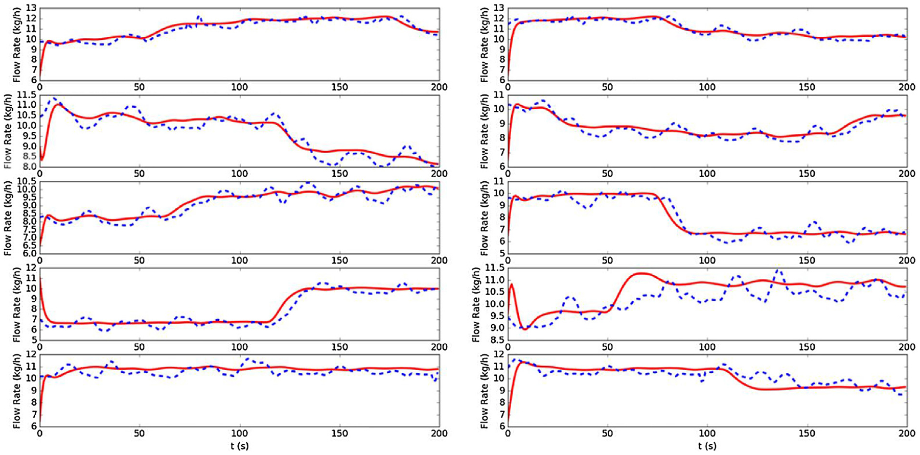
Measured (dashed line) and simulated (solid line) outlet mass flow rates.

3.3. Moving horizon problem formulation

In this work we first consider a pilot plant feeding–blending system where the API is fed from Feeder 1 (F1) and the excipient from Feeder 2 (F2). The API and excipient are mixed in Blender 1 (B1) and the mixture is conveyed to the next unit operation. Under the normal operation condition, the mass flow rate of the API is 1.0 kg/h and mass flow rate of the excipient is 9.0 kg/h.

State variables of this powder mixing system are defined as follows.

Measured variables
M F1	API mass hold-up of Feeder 1 (kg)
M F2	Excipient mass hold-up of Feeder 2 (kg)
ω F1	Screw rotation speed of Feeder 1 (rpm)
ω F2	Screw rotation speed of Feeder 2 (rpm)
F B1,out	Outlet mass flow rate of Blender 1 (kg/h)
C B1,out	Outlet API concentration of Blender 1
ω B1	Agitator rotation speed of Blender 1 (rpm)
Unmeasured Variables
F F1	Mass flow rate of Feeder 1 (kg/h)
F F2	Mass flow rate of Feeder 2 (kg/h)
F B1,in	Inlet mass flow rate of Blender 1 (kg/h)
C B1,in	Inlet API concentration of Blender 1
M B1,n	Mass hold-up of compartment n (kg)
F B1,n	Outlet mass flow rate of compartment n (kg/h)
C B1,n	Outlet API concentration of compartment n
Constants
${\omega }_F^{*}$, ${\omega }_{B1}^{*}$	Normal rotation speeds (rpm)
$M_F^{*}$, $M_{B1,n}^{*}$	Normal mass hold-ups (kg)
σ*, δ*	Variances of noise of state variables

For each feeder, the weight of materials in the hopper and the rotation speed of the screw are directly measured. Although the feed mass flow rate is also reported, it is not directly measured. Instead, the mass flow rate is calculated from differences in the weight measured by the load cell. For the continuous blender, the rotation speed of the agitator is directly measured. The outlet mass flow rate and the corresponding API concentration are indirectly measured by process analysis tools (PATs), such as X-ray and near-infrared (NIR) sensors. The resulting MHE problem formulation is given by

$$\begin{array}{ll}\text{min}\hfill & \sum _{t\in T_M}\sum _i\rho \left(\frac{X_i(t)-{\widehat{X}}_i(t)}{{\sigma }_i^{*}}\right)+{\sum _{t\in T_M}\sum _j\left(\frac{Z_i(t)-{\widehat{Z}}_j(t)}{{\delta }_j^{*}}\right)}^2\hfill \\ \text{s}.\text{t}.\hfill & \frac{d{M}_{F1}(t)}{dt}=-F_{F1}(t)\hfill \\ F_{F1}(t)={\alpha }_{F1}\frac{{\omega }_{F1}(t)}{{\omega }_{F1}^{*}}\left\{1+{\beta }_{F1}\frac{M_{F1}(t)}{M_{F1}^{*}}+{\gamma }_{F1}{\left[\frac{M_{F1}(t)}{M_{F1}^{*}}\right]}^2\right\}\hfill & \hfill \\ \frac{d{M}_{F2}(t)}{dt}=-F_{F2}(t)\hfill & \hfill \\ F_{F2}(t)={\alpha }_{F2}\frac{{\omega }_F(t)}{{\omega }_{F2}^{*}}\left\{1+{\beta }_{F2}\frac{M_{F2}\left(t\right)}{M_{F2}^{*}}+{\gamma }_{\text{F}2}{\left[\frac{M_{F2}\left(t\right)}{M_{F2}^{*}}\right]}^2\right\}\hfill & \hfill \\ F_{B1,in}(t)=F_{F1}(t)+F_{F2}(t)\hfill & \hfill \\ C_{B1,in}(t)=F_{F1}(t)+F_{B1,in}(t)\hfill & \hfill \\ F_{B1,0}(t)=F_{B1,in}(t)\hfill & \hfill \\ C_{B1,0}(t)=C_{B1,in}(t)\hfill & \hfill \\ \frac{d{M}_{B1,n}(t)}{dt}=F_{B1,n-1}(t)-F_{B1,n}(t)\hfill & \forall n\hfill \\ F_{B1,n}(t)={\alpha }_{B1}{\left[\frac{{\omega }_{B1}(t)}{{\omega }_{B1}^{*}}\right]}^{{\beta }_{B1}}{\left[\frac{M_{B1,n}(t)}{M_{B1,n}^{*}}\right]}^{{\gamma }_{B1}}\hfill & \forall n\hfill \\ \frac{d{C}_{B1,n}(t)}{dt}=\frac{F_{B1,n-1}(t)}{M_{B1,n}(t)}\left[C_{B1,n-1}(t)-C_{B1,n}(t)\right]\hfill & \forall n\hfill \\ F_{B1,N}(t)=F_{B1,out}(t)\hfill & \hfill \\ C_{B1,N}(t)=C_{B1,out}(t)\hfill & \hfill \end{array}$$ (11)

where t is continuous time, T_M is a set of time when state variables are measured, i is index of measured variables and j is index of unmeasured variables. The objective function consists of two parts, the robust state estimators for measured variables X and the least square regularization terms for unmeasured variables Z. In the robust estimators, X = [M_F1,M_F2,F_B1,out,C_B1,out,ω_F1,ω_F2,ω_B] is a vector of the measured variables, $\widehat{X}$ is a vector of the actual measurements, and σ* is a vector of the variances of measurement noise. The random measurement errors are assumed to be independent and normally distributed. The values of σ* are provided in Table 1. These values are determined from our observations in our pilot scale powder mixing process. In particular, for rotation speeds the values of normalized variance are very small. As a result, we assume rotation speeds are accurately measured and they are not considered in the objective function. For either feeder, the weight is measured by a load cell located below the hopper. The weight measurements are always contaminated with high-frequency random noise since even small vibrations can impact the weight readings. The outlet mass flow rate and the API concentration of the blender are indirectly measured by spectrum-based sensors. Measurements of spectra, such as X-ray or NIR, are also very sensitive to random noise.

Table 1 –

Variance values of random noise in the feeder and blender system.

	Absolute variance	Normalized variance
ω F1 , ω F2 , ω B	0.1	0.001
MF1 , MF2	0.01	0.05
F B1 , out	0.36	0.036
C B1,out	0.001	0.01

In this MHE case study we ignore the arrival function and assume there is no disturbance. We assume the robust estimator ρ(·) is time- and variable-independent. The same tuning constants are used for all case studies, for the Fair function c_F = 1.40, for the Logistic function c_Lo = 0.602, for the Welsch function c_W = 2.98, and for the Lorentzian function c_L = 2.60. These values are used in the literature (Ozyurt and Pike, 2004; Prata et al., 2008) where they are tuned for good performance of robust estimators. Although they may not be optimal for our particular case, previous work has shown that performance of robust estimators is not very sensitive to these parameter settings (Nicholson et al., 2014).

For unmeasured states M_B1,n and C_B1,n (n < N) we introduce least squares regularization terms in the objective function, where Z = [M_B1,1,…,M_B1,N−1,C_B1,1,…,C_B1,N−1] is a vector of unmeasured states, $\widehat{Z}$ is a vector of the state estimates, and δ* is a vector of the corresponding variance values. Note that these unmeasured states introduce degrees of freedom into the system. The regularization terms, given by

$$\sum _{t\in T_M}\sum _n{\left(\frac{M_{B1,n}\left(t\right)-{\widehat{M}}_{B1,n}\left(t\right)}{{\sigma }_{M,n}^{*}}\right)}^2+\sum _{t\in T_M}\sum _n{\left(\frac{C_{B1,n}\left(t\right)-{\widehat{C}}_{B1,n}\left(t\right)}{{\delta }_{C,n}^{*}}\right)}^2$$

impose penalties on differences between the current and previous estimates of these unmeasured states. Without loss of generality and for the sake of similarity in demonstrating numerical results, we consider 3 compartments in our “CSTR-in-series” model for the continuous blender. To complete the MHE problem formulation, the values of the parameters in our dynamic models are provided in Table 2.

Table 2 –

Parameter values of the dynamic model.

	Values		Values
αF1, αF2	1.11 × 10−5	α B	2.78 × 10−3
βF1, βF2	0.5	β B	1.0
γF1, γF2	−0.25	γ B	1.5

4. Results and discussions

In this section we test the proposed MHE framework on a simulation of the powder mixing system which consists of two feeders and one blender. Two major types of gross errors, outliers and measurement drifts, are introduced into our simulations. Four robust estimators, including the Fair function, the Logistic function, the Welsch redescending estimator, and the Lorentzian estimator, are compared with the traditional least squares function.

To better demonstrate the performance of different estimators, we focus on estimating eight key state variables: four measured variables including M_F1, M_F2, F_B1,out, and C_B1,out, and four unmeasured variables including M_B1,1, C_B1,1, M_B1,2, and C_B1,2. For the “CSTR-in-series” model with 3 compartments, these unmeasured states are necessary to describe the dynamics of the mass flow rate and AIP concentration. However, the state variables from the last compartment, M_B1,3 and C_B1,3, are not considered as they are already represented by F_B1,out and C_B1,out.

4.1. Solution strategy for MHE

From a mathematical point of view, the MHE problem (11) is a dynamic optimization (DO) problem constrained by differential algebraic equations (DAEs). Among different solution strategies, the simultaneous approach has been shown to offer good solution quality at acceptable computational cost (Biegler, 2007, 2010). In the simultaneous approach the DO problem is discretized with respect to time and the differential equations are approximated by polynomials. Different orthogonal collocation methods can be used to discretize the DAE system. The discretization of the original DO gives a well-defined nonlinear programming (NLP) problem with only algebraic constraints, which can be solved with general nonlinear optimizers.

The extended MHE framework is implemented in PYOMO, a flexible modeling language based on Python (Hart et al., 2017). In our simulations the time step is 1 s and the moving horizon includes 10 time steps. The MHE problem is discretized using the Radau collocation with 10 finite elements and 3 collocation points. Unless particularly mentioned, the same time horizon length and discretization scheme are used in all cases. The resulting large-scale NLP problem is solved with IPOPT, an open source nonlinear solver based on interior point algorithm (Wachter and Biegler, 2006). The computation is performed on a 64-bit MacBook Pro with CPU of Intel Core i5 @2.70 GHz and total memory of 16 GB.

4.2. Case study: outliers

Outliers are common gross errors, which usually have large measurement deviations but only exist for a short period of time. Outliers may be due to temporary sensor failures or signal transmission errors, and they should be excluded from the measurements. We first test the proposed MHE framework on measurements contaminated with outliers.

In our simulations the process is operated under the normal condition, where F_F1 = 1.0 kg/h and F_F2=9.0 kg/h. For the blender the outlet mass flow rate F_B1,out = 10 kg/h and the API concentration C_B1,out = 10.0%. The simulations are run for 250 time steps. Outliers are individually introduced to each measured state, M_F1, M_F2, F_B1,out, and C_B1,out, at time step 50, 100, 150, and 200, receptively. For each outlier the corresponding measurement deviation is significantly larger than the standard deviation of random noise.

Fig. 3 shows the actual measurements and the state estimates using different estimators. It is evident that even a single outlier can significantly contaminate the state estimates when the traditional least squares function is used. Particularly, when an outlier is introduced into F_B1,out or C_B1,out, we observe “smearing” effects: the estimates of unmeasured states M_B1,n or C_B1,n also drift away from true values. Moreover, the undesirable contamination can last for a long period of time even though the outlier is only present in one step. By contrast, the robust estimators perform much better than the least squares function. Since they are able to reduce or even eliminate the negative influences caused by the outliers, these robust estimators lead to more accurate estimates of all state variables. It can be noted that the performance of redescending estimators, the Welsch function and the Lorentzian function, are slightly better than the convex estimators in this particular case.

Fig. 3 –

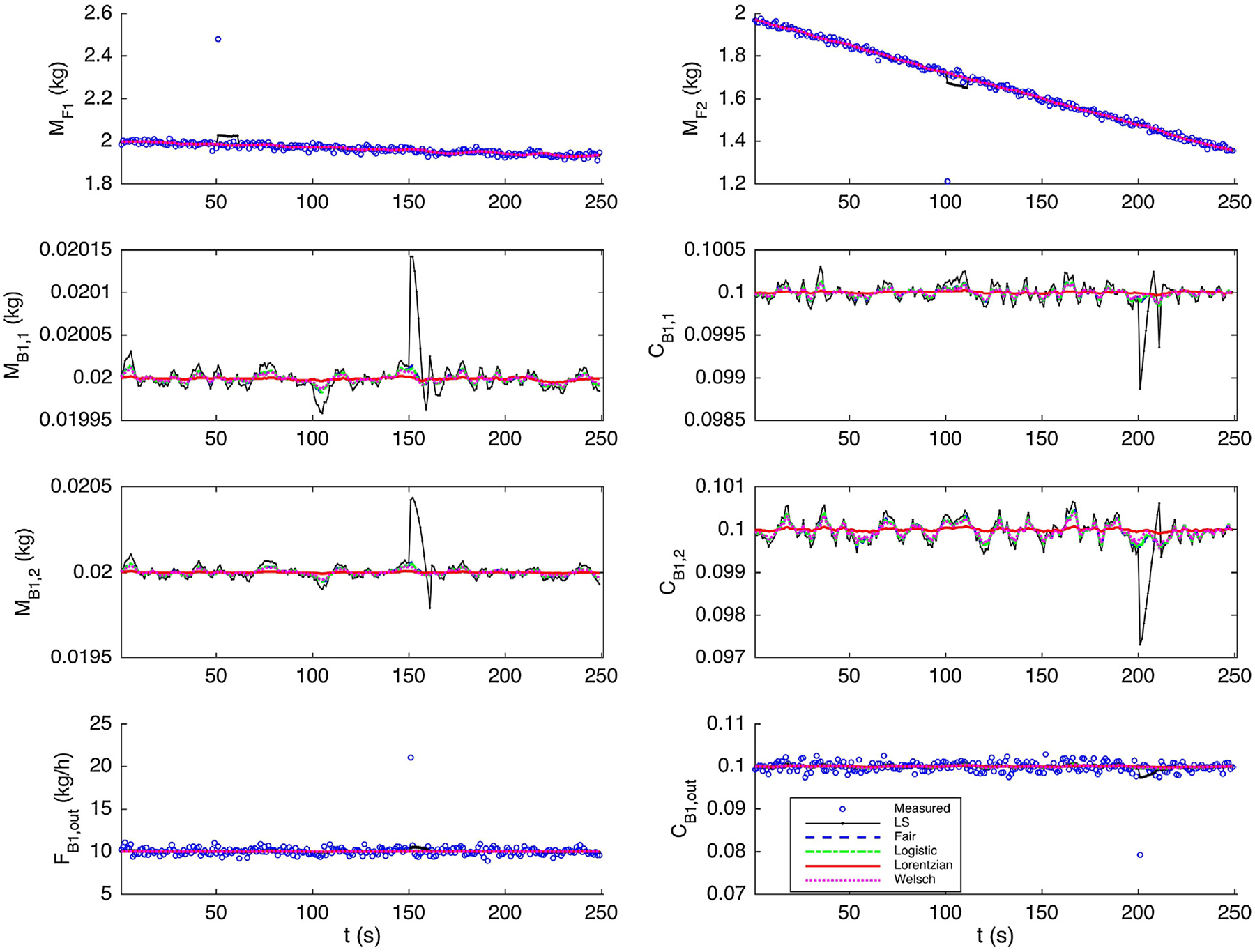
State estimates for measurements contaminated with outliers.

4.3. Case study: drifts

Measurement drifts and biases are persisting gross errors in measurements. Unlike outliers, drifts or bias may last for a long time and their deviations from true values, while usually much smaller than outliers, can be constant or changing gradually over time. They may be caused by improper installation of instruments, incorrect calibration of sensors, or inadequate maintenance. In our feeding–blending system the measurements from the X-ray and NIR sensors, are usually contaminated with drifts and bias. For instance, powder dust slowly building up on the probe can gradually reduce the accuracy of the spectrum measurement. Even if all measurement is error-free, imperfections in the regression models used in the process analysis tools (PATs) can also lead to biased interpretation of the current state.

In our simulations we consider measurement drifts in two state variables, the outlet mass flow rate F_B1,out and the API concentration C_B1,out, both of which are indirectly measured by spectrum-based sensors. In the first case we introduce a single drift into our simulations. The process is initially running under steady state at the normal condition. At time step 250 the set point of C_B1,out changes from 10.0% to 12.0% while the total flow rate remains the same value. A measurement drift is first introduced to F_B1,out at time step 60. The drift increases at a rate of 0.108 kg/h per time step and reaches the maximum error of 2.16 kg/h at time step 80. It stays at the maximum error level for 50 time steps before it decreases to zero at the same rate of 0.108 kg/h per time step. A similar drift is then introduced to C_B1,out shortly after the change of set point when the process is still under transition dynamics. This drift starts at time step 260, increases at a rate of 0.1% for 20 time steps, remains at the maximum error level for 50 time steps, and then decreases to zero at the same rate of 0.1%. The simulations are run for 400 time steps.

The actual measurements and state estimates are shown in Fig. 4. To better demonstrate performance of various estimators, we introduce the average estimation error as a quantitative metric. Here, the estimation error is defined as the absolute value of the difference between the true state and its estimate. To compute the average estimation error, we only consider the time periods when the measurement drifts are introduced. For the first measurement drift, we focus on average estimation errors of state variables M_B1,1, M_B1,2, and FB1,out from time step 60 to 150. For the second drift, we consider state variables C_B1,1, C_B1,2, and CB1,out from time step 260 to 350. The average estimation errors are shown in Table 3. It is clear that the performance of MHE with least squares is the worst, as the drifting errors cause inaccurate estimates of measured and unmeasured state variables. For instance, if drift is present in F_B1,out, the estimates of M_B1,1 and M_B1,2 are contaminated. Similarly, C_B1,1 and C_B1,2 are incorrectly estimated due to the presence of gross errors in C_B1,out. The convex robust estimators, the Fair function and the Logistic function, outperform the least squares function by reducing the undesirable smearing effects in both cases. However, the estimated values are still contaminated especially when there exist measurement drifts in C_B1,out. The redescending M-estimators, the Lorentzian function and the Welsch estimator, give the best performance. These estimators are minimally impacted by measurement drifts and give the most accurate state estimates.

Fig. 4 –

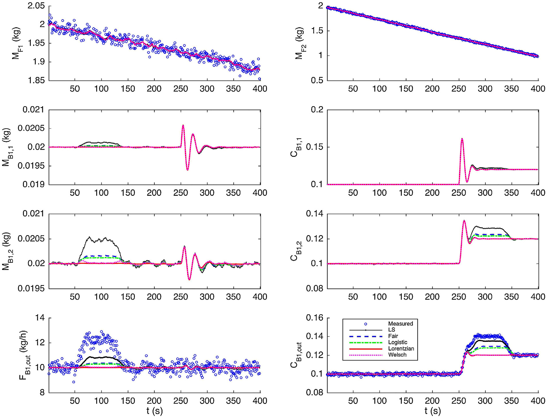
State estimates for measurements contaminated with single drift.

Table 3 –

Average estimation errors of selected state variables for single drift.

	Drift 1			Drift 2
	MB1,1	MB1,2	FB1,out	CB1,1	CB1,2	CB1,out
LS	0.0001	0.0004	0.6322	0.0016	0.0066	0.0116
Fair	0.0000	0.0001	0.2908	0.0005	0.0028	0.0073
Logistic	0.0000	0.0001	0.2421	0.0004	0.0019	0.0061
Lorentzian	0.0000	0.0000	0.0143	0.0000	0.0000	0.0001
Welsch	0.0000	0.0000	0.0620	0.0000	0.0001	0.0002

In practice multiple drifts may happen at the same time. To test the robustness of the proposed MHE framework, we introduce two overlapped drifts into the measurements. The drift in M_B1,out is the same as in the previous case. The drift in C_B1,out starts at time step 80, increases at the rate of 0.1% for 20 time steps, stays at the maximum error level for 50 time steps, and then decreases to zero at the same rate. The simulations are run under the normal operation condition for 230 time steps. Similar results are shown in Fig. 5. The average estimation errors, shown in Table 4, are computed for the time period from step 60 to 180. Again, the least squares function is the worst and the convex estimators perform significantly better. The redescending estimators give the best performance in this test case.

Fig. 5 –

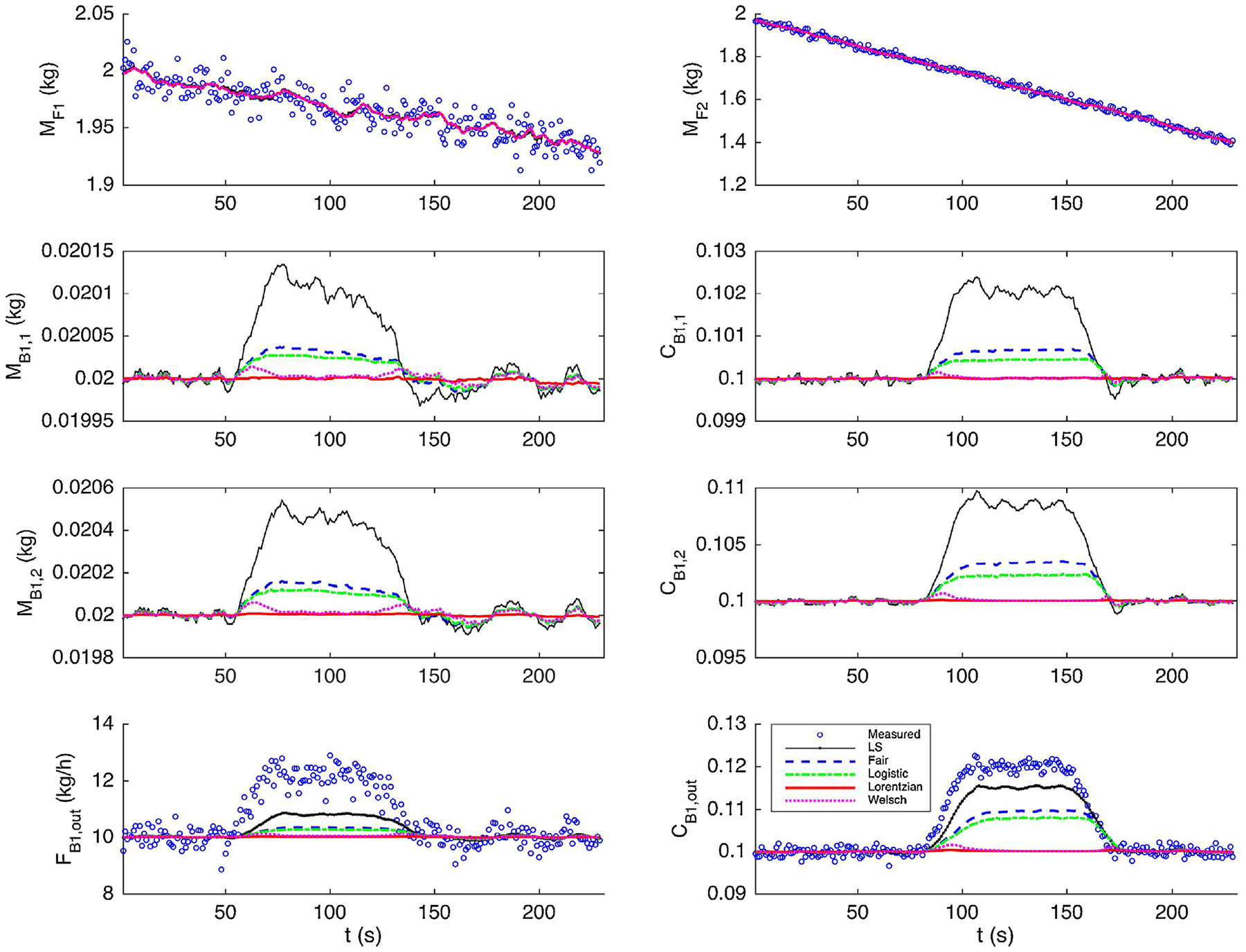
State estimates for measurements contaminated with multiple drifts.

Table 4 –

Average estimation errors of selected states for multiple drifts.

	MB1,1	MB1,2	FB1,out	CB1,1	CB1,2	CB1,out
LS	0.0001	0.0003	0.4808	0.0012	0.0051	0.0088
Fair	0.0000	0.0001	0.2190	0.0004	0.0021	0.0056
Logistic	0.0000	0.0001	0.1854	0.0003	0.0015	0.0047
Lorentzian	0.0000	0.0000	0.0127	0.0000	0.0000	0.0001
Welsch	0.0000	0.0000	0.0563	0.0000	0.0001	0.0003

4.4. Case study: control

Real-time state estimation is usually implemented to facilitate on-line monitoring, operation, and decision-making in continuous manufacturing processes. In particular, state estimation is crucial to advanced strategies relying on system models, such as model predictive control (MPC) and real-time optimization (RTO). To highlight the effect a state estimator has on the performance of an advanced process control, we integrate the proposed MHE within a nonlinear model predictive control (NMPC) framework. The structure of the control system is shown in Fig. 6.

Fig. 6 –

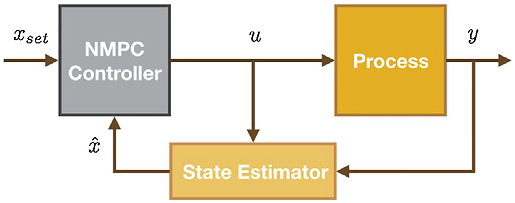
NMPC framework.

The controlled variables x are outlet mass flow rate F_B1,out and the API concentration C_B1,out. We use y to indicate the measurements of these two controlled variables. The manipulated variables u are the rotation speeds of screws in both feeders, ω_F1 and ω_F2. The state estimator takes the values of manipulated variables u and the measurements y to estimate the real values of the controlled variables x. The objective of the NMPC is to minimized the differences between the estimated controlled variables $\widehat{x}$ and the set point values x_set. To isolate the influence of gross errors, we assume no model-plan mismatch and use the same dynamic model of the feeding–blending system for the process simulator, state estimator, and the NMPC controller.

We consider the same simulation setting previously used in the cases with single drift in Section 4.3. However, the control decisions are now made based on the current state estimates provided by the state estimator. The simulation results are shown in Fig. 7. It is worthwhile to point out that all values plotted here are true state values without any noise or error. We can see that the MHE can significantly impact the performance of the controller. When the measurements are contaminated with gross errors, the MHE with least squares reports unreliable state estimates. Based on wrong information of the current state, the NMPC gives unnecessary control moves which force the controlled variables to drift away from the set-point values. In particular, for a positive measurement drift, the controller will decrease the controlled values in order to reduce the gaps between the incorrect state estimates and the step-point values. As a result, obvious negative drifts in true values of F_B1,out and C_B1,out arise as shown in Fig. 7. For convex robust estimators, the control of F_B1,out is not strongly impacted as measurement drift is correctly handled. However, the C_B1,out is not properly controlled due to the undesirable effects caused by gross errors. The redescending estimators, again, give the best performance when incorporated within an NMPC framework.

Fig. 7 –

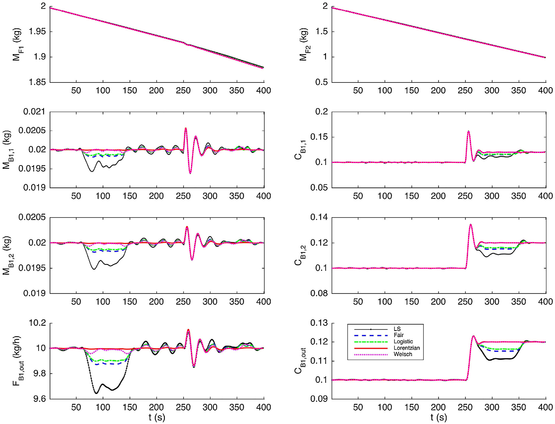
Performance of NMPC with different estimators.

4.5. Case study: system extension

To better demonstrate the proposed MHE framework, we consider a larger feeding–blending system with extensions in different aspects. First, we extend the feeding–blending system by introducing a third feeder (F3) and a second blender (B2). In particular, the lubricant (SiO₂) is fed from F3 with a normal flow rate of F_F3=0.05 kg/h. In the second blender B2, the lubricant is mixed with the powder (API and excipient) from the first blender B1. The mass flow rate (F_B2,out) and the AIP concentration (C_B2,out) are measured at the outlet of B2. In addition, we introduce 6 compartments in the blender models, leading to larger dynamic models with more intermediate, unmeasured states. In order to accommodate the extra residence time of the second blender, we use a longer moving horizon with duration of 30 s. As a result, the new dynamic system is significantly larger since more state variables are introduced by the additional equipment, more complex models, and larger time window. For the sake of simplicity, the same values of key parameters provided in Section 3.3 are used here.

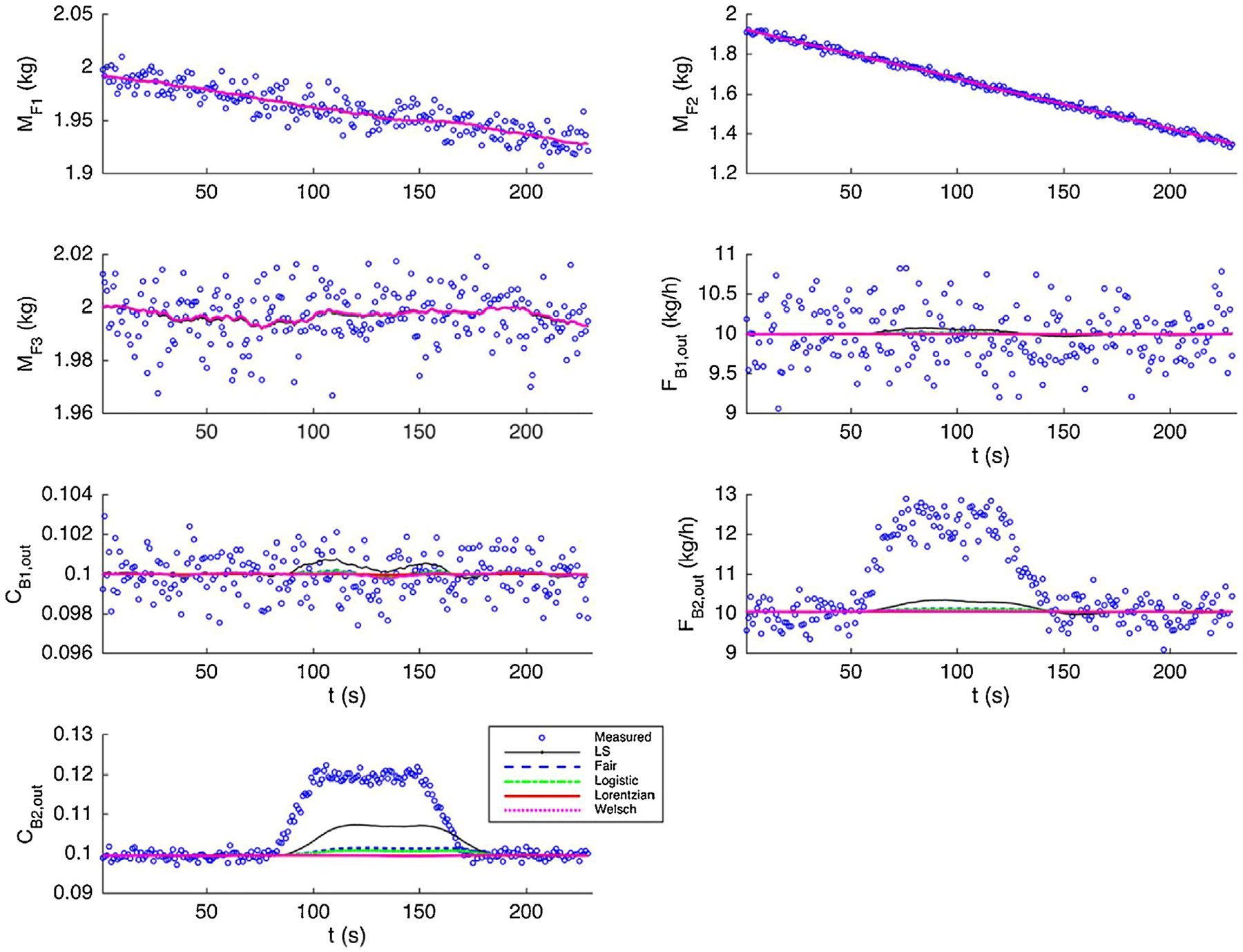
According to the previous results, all robust estimators considered in this work perform well in eliminating the impact of outliers. Therefore, in this extended case, we only focus on the performance of different robust estimators in handling measurement drifts. Similar patterns of measurements drifts as presented in Section 4.3 are used here. However, these drifts are introduced to the outlet flow rate and AIP concentration of the second blender B2.

For single measurement drift, the results are plotted in Fig. 8. The average estimation errors are shown in Table 5. Similarly, we focus on state variables F_B1,_out and F_B2,_out for the first measurement drift from time step 60 to 150. For the second drift, we only consider the average estimation errors of C_B1,_out and C_B2,_out from time step 260 to 350.

Fig. 8 –

State estimates for measurements contaminated with single drift in the extended system.

Table 5 –

Average estimation errors of selected state variables for single drift in extended system.

	Drift 1		Drift 2
	FB1,out	FB2,out	CB1,out	CB2,out
LS	0.0479	0.2144	0.0004	0.0056
Fair	0.0116	0.0596	0.0001	0.0015
Logistic	0.0088	0.0456	0.0001	0.0010
Lorentzian	0.0007	0.0026	0.0000	0.0000
Welsch	0.0028	0.0079	0.0001	0.0001

It can be readily seen that the state estimates of least squares function can be strongly impacted by measurement drifts. The robust estimators, however, can significantly reduce the negative impact caused by measurement drifts.

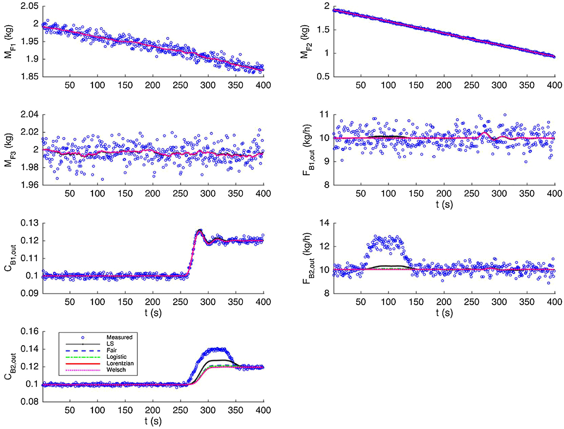
The results of multiple measurement drifts are plotted in Fig. 9. The average estimation errors are shown in Table 6 where we only consider the time period from step 60 to 180. Again, the least squares alternative leads to poor state estimates when there exist multiple measurements. The robust estimators lead to similar performance. In particular, the redescending estimators Lorentzian and Welsch give the best state estimates.

Fig. 9 –

State estimates for measurements contaminated with multiple drifts in the extended system.

Table 6 –

Average estimation errors of selected state variables for multiple drifts in extended system.

	FB1,out	FB2,out	CB1,out	CB2,out
LS	0.0373	0.1514	0.0003	0.0044
Fair	0.0102	0.0464	0.0001	0.0012
Logistic	0.0080	0.0362	0.0001	0.0008
Lorentzian	0.0008	0.0024	0.0000	0.0000
Welsch	0.0032	0.0079	0.0001	0.0001

4.6. Computational results

In this section, we summarize the computational performance of the MHE framework for the basic and extended feeding–blending systems. The basic system consists of two WIL feeders and one continuous blender. In the MHE problem formulation, we consider three compartments in the blender model and the moving window is 10 s. The extended system, which is built on the basic one, consists of three feeders and two blenders. In addition, we introduce six compartments in the blender models and the moving window is extended to 30 s. For both basic and extended systems, the dynamic optimization problems are discretized using the orthogonal collocation method, leading to large-scale nonlinear programming problems. Table 7 shows the size and computational time of these optimization problems, where the ‘Variable’ column indicates the number of variables in the nonlinear program, the ‘Constraints’ column indicates the number of (equality and inequality) constraints in the nonlinear program, and the ‘Time’ column shows the average computational time in solving each MHE problem. Note that the size of formulations with Fair and Logistic estimators are slightly larger, since the representation of absolute residual requires more intermediate variables and inequality constraints.

Table 7 –

Size and computational time of discretized MHE problems for basic and extended systems.

	Basic system			Extended system
	Variables	Constraints	Time (s)	Variables	Constraints	Time (s)
LS	811	793	0.03	5992	5939	0.22
Fair	881	855	0.05	6209	6373	0.46
Logistic	881	855	0.05	6209	6373	0.48
Lorentzian	811	793	0.03	5992	5939	0.23
Welsch	811	793	0.03	5992	5939	0.24

In both cases, the MHE problem can be efficiently solved within the sampling time interval which is one second. However, the average computational time increases as the size of problem increases.

To indicate the impact of time horizon, we consider two more time windows for the extended system. The size and computational time of the resulting MHE problems are given in Table 8. It is clear to see that longer time horizons lead to larger optimization problems, which can be more challenging to solve due to more variables and constraints. However, it is worthwhile to point out that the solution of the NMPC formulation requires in excess of 20 s. Therefore, the time window of 30 s for the MHE is a suitable compromise selection from the point of view of both control performance and computational efficiency.

Table 8 –

Size and computational time for extended system with different time horizons.

	Extended system, Horizon = 20 s			Extended system, Horizon = 40 s
	Variables	Constraints	Time (s)	Variables	Constraints	Time (s)
LS	4032	3979	0.16	7952	7899	0.31
Fair	4179	4273	0.30	8239	8473	0.68
Logistic	4179	4273	0.31	8239	8473	0.69
Lorentzian	4032	3979	0.17	7952	7899	0.32
Welsch	4032	3979	0.17	7952	7899	0.34

5. Conclusions

Real-time state estimation plays a crucial role in on-line monitoring and control of continuous pharmaceutical manufacturing. The moving horizon estimation (MHE) approach has been extensively studied and widely used in various applications since it is well suitable for nonlinear systems with hard constraints. Recent development in numerical methods and solution strategies makes it possible to solve the large-scale MHE problem efficiently. Traditional MHE approaches assume random measurement noise governed by some normal distribution. However, this assumption is not always valid since the actual distributions are often unknown or exhibiting departures from normal form. In addition, conventional state estimators fail to consider gross or systematic errors, such as bias, outliers, and drifts. The presence of gross errors can contaminate the state estimates and the reconciled measurements, causing undesirable “smearing” effects. As a result, research on state estimation is closely related to topics of data reconciliation (DR) and gross error detection (GED).

Inspired by related work in DR and GED, we incorporate robust estimators within the classic MHE skeleton, giving an extended MHE framework which is suitable for dynamic systems with gross errors. In particular, we consider four robust estimators from two major categories, the convex estimators, such as the Fair and Logistic functions, and the redescending M-estimators, such as the Welsch and Lorentzian functions. We test the proposed MHE framework on a simple feeding–blending system (FBS) configuration which includes two loss-in-weight (LIW) feeders and one continuous blender. However, previous modeling strategies of the powder mixing process are not practical for use in our MHE framework. Therefore, a reduced-order dynamic model is proposed for the LIW feeder, where the mass flow rate is a function as screw rotation speed and mass hold-up in the hopper. We also introduce a “CSTR-in-series” model for the continuous blender, where the blender is separated into a number of ideal CSTRs as compartments.

To illustrate the performance of our MHE framework, we introduce gross errors, including outliers and single and multiple measurement drifts, into our simulations of the powder mixing system. Numerical results show significant benefits in applying our MHE framework with robust estimators. Compared with the conventional least squares function, robust estimators can indeed reduce the smearing effects caused by gross errors, leading to more accurate and reliable estimates of the current state of the system. Furthermore, the proposed MHE is integrated into a model predictive control (MPC) framework to show the impact of state estimation on the performance of advanced process control. The redescending estimators, the Welsch and Lorentzian functions, give the best performance among all robust estimators considered in this work and the resulting optimization problems can be efficiently solved. The MHE framework is also tested on a larger FBS consisting of three LIW feeders and two continuous blenders. Computational results indicate that the MHE problem can be efficiently solved in real time.

In the future we will implement the proposed MHE framework to a pilot plant FBS which is part of a continuous dry granulation line and demonstrate the on-line state estimation capabilities. This requires further effort at improving solution reliability and robustness, reducing solution time, integrating MHE with advanced monitoring and control strategies, and dynamic parameter estimation of process models. The proposed MHE framework will also be tested on the complete dry granulation based continuous tableting line.

References

- Abrol Sidharth, Edgar Thomas F., 2011. A fast and versatile technique for constrained state estimation. J. Process Control 21 (3), 343–350. [Google Scholar]
- Albuquerque Joao S., Biegler Lorenz T., 1996. Data reconciliation and gross-error detection for dynamic systems. AIChE J 42 (10), 2841–2856. [Google Scholar]
- Arora Nikhil, Biegler Lorenz T., 2001. Redescending estimators for data reconciliation and parameter estimation. Comput. Chem. Eng 25 (11), 1585–1599. [Google Scholar]
- Arulmaran Kevin, Liu Jinfeng, 2017. Handling model plant mismatch in state estimation using a multiple-model-based approach. Ind. Eng. Chem. Res 56 (18), 5339–5351. [Google Scholar]
- Arulampalam M. Sanjeev Maskell Simon,Gordon Neil, Clapp Tim, 2002. A tutorial on particle filters for online nonlinear/non-gaussian bayesian tracking. IEEE Trans. Signal Process 50 (2), 174–188. [Google Scholar]
- Biegler Lorenz T., 2007. An overview of simultaneous strategies for dynamic optimization. Chem. Eng. Process.: Process Intensif 46 (11), 1043–1053. [Google Scholar]
- Biegler Lorenz T., 2010. Nonlinear Programming: Concepts, Algorithms, and Applications to Chemical Processes, vol. 10. Siam. [Google Scholar]
- Boukouvala Fani, Dubey Atul, Vanarase Aditya, Ramachandran Rohit, Muzzio Fernando J., Ierapetritou Marianthi, 2012. Computational approaches for studying the granular dynamics of continuous blending processes, 2–population balance and data-based methods. Macromol. Mater. Eng 297 (1), 9–19. [Google Scholar]
- Bourouis Mahmoud, Pibouleau Luc, Floquet Pascal, Domenech Serge, AlGobaisi Darwish M.K., 1998. Simulation and data validation in multistage flash desalination plants. Desalination 115 (1), 1–14. [Google Scholar]
- Bryson Arthur Earl, 1975. Applied Optimal Control: Optimization, Estimation and Control CRC Press. [Google Scholar]
- Chen Xueyu, Pike Ralph W., Hertwig Thomas A., Hopper Jack R., 1998. Optimal implementation of on-line optimization. Comput. Chem. Eng 22, S435–S442. [Google Scholar]
- Cleary Paul W., 2007. Dem modelling of particulate flow in a screw feeder model description. Prog. Comput. Fluid Dyn 7 (2–4), 128–138. [Google Scholar]
- Dennis John E., Welsch Roy E., 1978. Techniques for nonlinear least squares and robust regression. Commun. Stat. Simul. Comput 7 (4), 345–359. [Google Scholar]
- Dubey Atul, Sarkar Avik, Ierapetritou Marianthi, Wassgren Carl R., Muzzio Fernando J., 2011. Computational approaches for studying the granular dynamics of continuous blending processes, 1–DEM based methods. Macromol. Mater. Eng 296 (3–4), 290–307. [Google Scholar]
- Fair Ray C., 1974. On the robust estimation of econometric models. Annals of Economic and Social Measurement, vol. 3., pp. 667–677, NBER number 4. [Google Scholar]
- Fuente MJ ,Gutierrez G, Gomez E, Sarabia D, de Prada C, 2015. Gross error management in data reconciliation. 9th Internafional Symposium on Advanced Control of Chemical Processes. [Google Scholar]
- Gao Yijie, Vanarase Aditya, Muzzio Fernando, Ierapetritou Marianthi, 2011. Characterizing continuous powder mixing using residence time distribution. Chem. Eng. Sci 66 (3), 417–425. [Google Scholar]
- Hart William E., Laird Carl, Watson Jean-Paul, Woodruff David L., 2017. Pyomo–Optimization Modeling in Python, vol. 67, Second edition Springer Science & Business Media. [Google Scholar]
- Haseltine Eric L., Rawlings James B., 2005. Critical evaluation of extended kalman filtering and moving-horizon estimation. Ind. Eng. Chem. Res 44 (8), 2451–2460. [Google Scholar]
- Houtekamer Peter L., Mitchell Herschel L., 1998. Data assimilation using an ensemble kalman filter technique. Mon. Weather Rev 126 (3), 796–811. [Google Scholar]
- Hu Guoming, Chen Jinxin, Jian Bin, Wan Hui, Liu Lipin., 2010. Modeling and simulation of transportation system of screw conveyors by the discrete element method. Mechanic Automation and Control Engineering (MACE), 2010 International Conference on, 927–930, IEEE. [Google Scholar]
- Imole Olukayode I., Krijgsman Dinant, Weinhart Thomas, Magnanimo Vanessa, Chavez Montes Bruno E., Ramaioli Marco, Luding Stefan, 2016. Experiments and discrete element simulation of the dosing of cohesive powders in a simplified geometry. Powder Technol 287, 108–120. [Google Scholar]
- Johnston Lloyd P.M., Kramer Mark A., 1995. Maximum likelihood data rectification: steadystate systems. AIChE J 41 (11), 2415–2426. [Google Scholar]
- Julier Simon, Uhlmann Jeffrey, Durrant-Whyte Hugh F., 2000. A new method for the nonlinear transformation of means and covariances in filters and estimators. IEEE Trans. Automat. Control 45 (3), 477–482. [Google Scholar]
- Llanos Claudia E., Sanchez Mabel C., Maronna Ricardo A., 2015. Robust estimators for data reconciliation. Ind. Eng. Chem. Res 54 (18), 5096–5105. [Google Scholar]
- Marikh K, Berthiaux H, Mizonov V, Barantseva E, Ponomarev D, 2006. Flow analysis and markov chain modelling to quantify the agitation effect in a continuous powder mixer. Chem. Eng. Res. Des 84 (11), 1059–1074. [Google Scholar]
- Nicholson Bethany, Lopez-Negrete Rodrigo, Biegler Lorenz T., 2014. On-line state estimationí of nonlinear dynamic systems with gross errors. Comput. Chem. Eng 70, 149–159. [Google Scholar]
- Ozyurt Derya B., Pike Ralph W., 2004. Theory and practice of simultaneous data reconciliation̈ and gross error detection for chemical processes. Comput. Chem. Eng 28 (3), 381–402. [Google Scholar]
- Prata Diego Martinez, Pinto Jose Carlos, Lima Enrique Luis, 2008. Comparative analysis of robust estimators on nonlinear dynamic data reconciliation. Comput. Aided Chem. Eng 25, 501–506. [Google Scholar]
- Ramlal Jasmeer, Allsford Kenneth V., Hedengren John D., 2007. Moving horizon estimation for an industrial gas phase polymerization reactor. IFAC Proc Vol. 40 (12), 1040–1045. [Google Scholar]
- Rao Christopher V., Rawlings James B., Mayne David Q., 2003. Constrained state estimation for nonlinear discrete-time systems: Stability and moving horizon approximations. IEEE Trans. Automat. Control 48 (2), 246–258. [Google Scholar]
- Rehrl Jakob, Kruisz Julia, Sacher Stephan, Khinast Johannes, Horn Martin, 2016. Optimized continuous pharmaceutical manufacturing via model-predictive control. Int. J. Pharm 510 (1), 100–115. [DOI] [PubMed] [Google Scholar]
- Sen Maitraye, Ramachandran Rohit, 2013. A multi-dimensional population balance model approach to continuous powder mixing processes. Adv. Powder Technol 24 (1), 51–59. [Google Scholar]
- Sen Maitraye, Singh Ravendra, Sen Maitraye, Ramachandran Rohit, 2013. Mathematical development and comparison of a hybrid pbm-dem description of a continuous powder mixing process. J. Powder Technol, 2012. [Google Scholar]
- Singh Ravendra, Ierapetritou Marianthi, Ramachandran Rohit, 2013. System-wide hybrid MPC–PID control of a continuous pharmaceutical tablet manufacturing process via direct compaction. Eur. J. Pharm. Biopharm 85 (3), 1164–1182. [DOI] [PubMed] [Google Scholar]
- Tjoa IB, Biegler LT, 1991. Simultaneous strategies for data reconciliation and gross error detection of nonlinear systems. Comput. Chem. Eng 15 (10), 679–690. [Google Scholar]
- Vachhani Pramod, Rengaswamy Raghunathan, Gangwal Vikrant, Narasimhan Shankar, 2005. Recursive estimation in constrained nonlinear dynamical systems. AIChE J 51 (3), 946–959. [Google Scholar]
- Vachhani Pramod, Narasimhan Shankar, Rengaswamy Raghunathan, 2006. Robust and reliable estimation via unscented recursive nonlinear dynamic data reconciliation. J. Process Control 16 (10), 1075–1086. [Google Scholar]
- Wachter Andreas, Biegler Lorenz T., 2006. On the implementation of an interior-point filter̈ line-search algorithm for large-scale nonlinear programming. Math. Program 106 (1), 25–57. [Google Scholar]