Generative adversarial networks and image-based malware classification

Abstract

For efficient malware removal, determination of malware threat levels, and damage estimation, malware family classification plays a critical role. In this paper, we extract features from malware executable files and represent them as images using various approaches. We then focus on generative adversarial networks (GAN) for multiclass classification and compare our GAN results to other popular machine learning techniques, including support vector machine (SVM), XGBoost, and restricted Boltzmann machines (RBM). We find that the AC-GAN discriminator is generally competitive with other machine learning techniques. We also evaluate the utility of the GAN generative model for adversarial attacks on image-based malware detection. While AC-GAN generated images are visually impressive, we find that they are easily distinguished from real malware images using any of several learning techniques. This result indicates that our GAN generated images are of surprisingly little value in adversarial attacks.

Introduction

The Covid-19 pandemic, which ran amok worldwide for more than two years, drastically increased the trend of working from home. The remote work environment has also pushed another trend: increasing cyber attacks, including phishing, data breaches, and malware. According to CSO [8], in the second quarter of 2020, as compared to the same period a year earlier, cloud security incidents increased by 188%, ransomware attacks grew by over 40%, and email malware attacks were up by 600%.

Malware, short for “malicious software”, consists of computer programs that are written to cause harm to computer and Internet users [39]. Common types of malware include botnets, rootkits, Trojans, worms, and spyware. Malware can be used to steal information, utilize hardware, cause disruption for financial or reputational gain, or other unauthorized activity. Malware defense is an ongoing battle with multiple layers: preventing malware from entering, alerting users that a system is compromised, removal of malware from compromised systems, and so on.

There has been considerable research into malware detection and classification. In recent years, malware classification based on machine learning has become the leading focus of such research. With more computing power from graphic processing units (GPU) and Google tensor processing units (TPU), which are specialized for machine learning techniques and feature extraction, costly deep learning image-based malware detection techniques have become a viable option.

An image can be derived directly from the byte sequence of an executable file without executing (or emulating) or otherwise pre-processing the data to extract features. Powerful image-based techniques, including Convolutional Neural Networks (CNN) and Generative Adversarial Networks (GAN) have been used to classify malware samples with impressive results.

Malware detection is an arms race between detectors and malware writers, where each side tries to develop new and innovative ways to defeat the other side. Adversarial attacks on machine learning based malware defenses have been developed. In one type of adversarial attack, a malware writer attempts to contaminate the training data, so that the resulting model is less effective. A possible approach to such an adversarial attack on an image-based malware detection system is to generate “deep fake” malware images to pollute the training dataset. This is an approach that we consider in this paper.

GANs have been used to generate realistic fake images. For example, researchers at Nvidia [26] developed StyleGAN, a style-based architecture for GAN, which by some measures was 20% more effective than a traditional GAN generator. StyleGAN was also used to create the trending website “thispersondoesnotexist.com”. MalGAN is a GAN technique that was designed specifically to deal with malware images [22, 27]. In this paper, we consider the utility of GANs for adversarial attacks on image-based malware systems.

In addition to malware detection, malware classification is critically important, as it enables us to estimate the damage, determine the threat level, and to provide protection specific to a given malware family. In this research, we employ Auxiliary Classifier GAN (AC-GAN) for multi-class classification of malware families and compare the resulting model with a wide variety of other machine learning models, including Support Vector Machine (SVM) [19], k-Nearest Neighbors (k-NN) [20], multilayer perceptron (MLP) [44], Random Forest (RF) [17], Restricted Boltzmann Machines (RBM) [29], XGBoost [10], as well as the pre-trained deep residual network, Resnet152 [18]. We also develop SVM and RF models to test the quality of fake images generated by our AC-GAN generative model. The dataset that we use consists of more than 26,000 malware executables from 20 distinct families [12].

Among the contributions of this paper are the following.

• We compare four distinct techniques for generating images from malware samples. Both grayscale and color images are considered. As far as the authors are aware, no previous work has provided a direct comparison of all of the image generation techniques considered in this paper.

• We apply a wide variety of learning techniques to a challenging malware image classification problem. In each case, we carefully tune the hyperparameters, which results in a meaningful comparison of these learning techniques in the image-based malware classification domain. The only comparable work that the authors are aware of is [37], which is focused on sequential techniques, including Long Short-Term Memory (LSTM) and Gated Recurrent Unit (GRU) classifiers.

• We carefully consider the potential utility of GAN-generated “deep fake” malware images for adversarial attacks. While such deep fake images are indeed visually impressive, we find that they are woefully inadequate for adversarial attacks. Specifically, we find that these deep fake images cannot serve as substitutes for actual malware images in adversarial attack scenarios. The authors are not aware of any previous work that explicitly makes this point, with the possible exception of [32], which is primarily focused on the classification potential of GANs, rather than their use in adversarial attacks.

The remainder of this paper is organized as follows. In Sect. 2, we discuss related work and briefly consider each of the various machine learning and deep learning models used in our research. Our dataset and image extraction techniques are introduced in Sect. 3. In Sect. 4, we present our extensive experimental results, and we provide analysis and discussion of these results. Section 5 concludes the paper, and we outline a few potential avenues for future work.

Background

New malware families are being developed everyday. For example, not too long ago the SolarWinds zero day attack caused damage to several government agencies [30]. The attack was caused by a state-sponsored group and put the entire cyber security industry on high alert. The SolarWinds attack reminded us of the importance of malware defense, and malware detection in particular.

There are two broad categories of malware detection: signature-based and anomaly-based. Signature-based malware detection keeps certain characteristics of previously-seen malware in a dictionary and detects based on this previously-determined information. There are three main disadvantages of a signature-based approach, namely, the size of the dictionary may not be scalable, new malware or zero day attacks cannot be detected, and signatures can be changed by malware writers using well-known obfuscation techniques. Anomaly-based detection tries to distinguish between benign and malware based on general characteristics or behavior. One disadvantage of anomaly-based detection is that if the training dataset can be corrupted in an adversarial fashion, anomalous features can be made to appear normal.

Machine learning techniques can be viewed as a type of anomaly-based detection, and such techniques can also be considered as higher-level “signatures,” in the sense that a model captures characteristics of an entire family, rather than a single instance. Regardless of how we view machine learning models, adversarial attacks are a major concern. One purpose of our research is to consider the effectiveness of generated fake malware images in such adversarial attacks—with the ultimate goal of producing more robust learning models.

Next, we discuss relevant related work. Then we briefly introduce each of the learning techniques considered in this paper. We conclude this section with a discussion of the statistics used to quantify classification success in our experiments.

Related work

As a first example of research in image-based analysis, Jain and Stamp [24] used Convolutional Neural Networks (CNN) and Extreme Learning Machines (ELM) to classify malware. Jain and Stamp suggested future work including testing different techniques for image extraction, such as zero padding and GIST descriptors of images.

In another paper, Nagaraju and Stamp [32] worked on image-based malware analysis using the GAN architecture known as Auxiliary-Classifier GAN(AC-GAN). They experimented with different image sizes from $32\times 32$, $64\times 64$ to as large as $512\times 512$. Grayscale images were extracted and truncated from executable files to the desired sizes. In addition to AC-GAN, CNN and ELM were considered, with CNN achieving impressive results in detecting fake images. For future work, they advised researchers to consider cutting-edge models, including VG-199 and ResNet152.

Xiao et al. [52] introduced a novel framework called MalCVS, which is their shorthand for Malware Classification using Colab image generation, VGG16, and SVM. Images were generated similar to grayscale, but with thick colored lines between each section in the executable files. The images then were passed through VGG16 for feature extraction with the results fed to a multi-class SVM for classification. The MalCVS framework achieved impressive results with 98.94% accuracy and F1-score at 97.91% on a multiclass (16 family) problem. Note that the MalCVS framework depart from strict grayscale images by its use of color borders in its image representation of malware.

A recent trend in image-based malware analysis is the use of color images. Both Vasan et al. [47] and Singh et al. [43] generate color maps and use byte sequences from the executable files to represent color images. Both papers also use similar learning techniques, including CNN and Residual Neural Networks (specifically, ResNet-50). Singh et al. achieved impressive results with the MalImg dataset, obtaining an accuracy of 98.10% using ResNet-50, while Vasan et al. attained an accuracy of 98.82% using a so-called “fine-tuned” CNN architecture. These papers tend to indicate that color (RGB) representations captured more pattern information, and therefore can achieve better results as compared to grayscale malware images.

The idea of generating fake features for obfuscation and adversarial attacks on malware systems is not new. For example, Hu et al. [22] and Kawai et al. [27] proposed MalGAN to bypass black-box machine learning based detection models. MalGAN uses the output of a black-box model and employs GAN to generate fake samples. MalGAN has been shown to be capable of substantially decreasing the true positive rate (TPR) to near 0. The process of training MalGAN is fast and efficient, making it practical for such attacks.

In the area of multiclass classification, Fu et al. [16] achieved impressive results with a accuracy of 97.47% and F-measure of 96.85% in categorizing 15 different malware families. They focused heavily on extracting features from malware executables, with a combination of global and local features. Color features were extracted using a Portable Executable (PE) format parser, and color images were built using RGB layers. The executable files were divided into sections, with features such as entropy, byte sequences, relative size, and so on, extracted per section. The results were then combined to represent the different RGB channels. The resulting images were colorful and enable us to visualize the data and code sections in malware files. For future work, they suggested that deep learning models such as CNN could be developed for malware classification.

Farhat and Rammouz [15] experimented with several pre-trained deep convolutional models, including VGG16, Resnet50, Resnet152, and MobileNet. With MobileMet, for example, they obtained an accuracy of 94% after one training epoch, based on a 9-class malware classification problem. After 25 epochs, the accuracy reached a peak of more than 97%. Pre-trained models take advantage of powerful image-based techniques and have been trained on vast datasets, while only requiring fine tuning for the specific task at hand. Thus, we can use pre-trained models for computer vision tasks and save a tremendous amount of training time.

In our research, we consider a wide variety of machine learning techniques, specifically, SVM, k-NN, MLP, RBM, and two ensemble techniques:, namely, Random Forest and XGBoost. We also consider three deep learning models: DC-GAN, AC-GAN, and Resnet152. In the next section, we briefly discuss each of these techniques, and we mention the relative advantages and disadvantages of each in the context of image-based malware classification.

Machine learning models

As its name suggests, the k-Nearest Neighbors (k-NN) classifier simply uses the k neighbors in the training set to classify a sample in the test set. Consequently, k-NN is simple and easy to understand, and it perform surprisingly well in many applications. However, with images of size $128\times 128\times 3$, for example, the feature vector would be of length 49,152, making distance computations in k-NN costly.

Support Vector Machines (SVM) and its multiclass version, Support Vector Classifiers (SVC), use hyperplanes to separate and classify data. Figure 1 illustrates a 2D version of SVM hyperplane—in this case, a line separating two classes of data. SVM performs well on many malware problems; for example, SVM achieved 93.20% accuracy on a 25-class classification problem in [47]. However, similar to k-NN, when the feature space is large, SVM can be quite costly in practice.

Fig. 1.

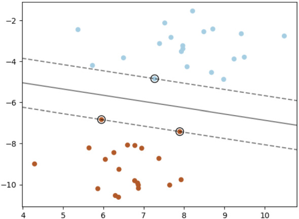
SVM separating hyperplane [46]

We also consider two ensembles: Random Forest (RF) and XGBoost. An ensemble is a group of models that are combined in some way to function as a whole. XGBoost requires substantial memory, as the dataset needs to be preprocessed before training.

Deep learning models

Generative Adversarial Networks (GAN) are innovative techniques where a generative and discriminative model are trained simultaneously. The two models compete with each other, and thus can yield improved results, as compared to training each individually. There are many GAN variants, including ProGAN, StyleGAN, and so on. We experiment with DC-GAN for unsupervised generative models and AC-GAN for multi-class discrimination. A primary goal for this research is to examine both the discriminator and the generator models of GANs and compare them with various other machine learning and deep learning techniques. The AC-GAN discriminator can be used for the multiclass classification of malware families and binary classification of fake versus real images. The GAN generator is used to produce fake malware images, which we analyze using various other learning techniques.

Additionally, we consider Restricted Boltzmann Machines (RBM) and the deep Residual Network (ResNet) architecture known as Resnet152. The Resnet152 model has been pre-trained on a vast image dataset and this particular model has been shown to achieve state-of-the-art results for malware problems. Next, we briefly introduce each of these deep learning models.

Deep convolutional GAN (DC-GAN)

DC-GAN was first introduced by Radford and Metz [38] in 2015 as an unsupervised technique for representational learning. As an unsupervised architecture, DC-GAN is applicable to unlabelled data. We use our DC-GAN results as a benchmark for the binary classification of real versus fake malware images.

Figure 2 illustrates the convolutional layers of a DC-GAN architecture without fully connected or pooling layers. Here, a noise vector consisting of 100 random numbers is fed into the model, which then generates images based on the training data. The basic architecture of our DC-GAN has four convolutional layers and the output is a $64\times 64\times 3$ image. We can modify the settings in the convolutional layers to work with all of the image types considered in our experiments below, namely, $128\times 128\times 1$ and $256\times 256\times 1$ grayscale, as well as $128\times 128\times 3$ RGB images.

Fig. 2.

DC-GAN generator [38]

Auxiliary-classifier GAN (AC-GAN)

There are multiple research papers showing that AC-GAN performs well with multiclass data [25, 32, 34]. In contrast to DC-GAN, AC-GAN makes use of class labels. Using this extra data (the class labels), also enables us to generate fake samples corresponding to a specific family. The AC-GAN discriminator can be used to solve the multiclass classification problem, which is a main focus in this research.

As we can see in Fig. 3, the input C, representing class labels, is fed into both the generator and the discriminator. There are two outputs from the discriminator, namely, the validity of the image and the class label. The discriminator is trained based on these two outputs, with two loss functions.

Fig. 3.

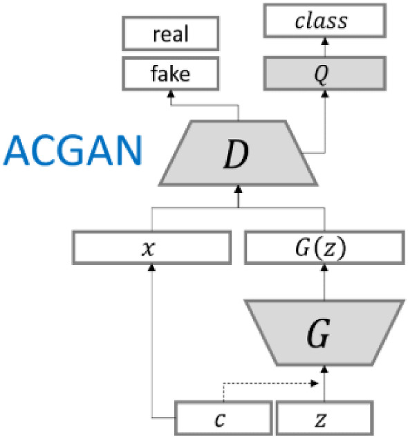
AC-GAN architecture [50]

Restricted Boltzmann machines

Restricted Boltzmann Machines (RBM) can extract non-linear features from images, which can then be used by a linear model, such as Logistic Regression (LR). In some applications, RBMs perform well; for example, an RBM with an LR classifier has achieved 94% accuracy for the handwritten digit classification problem [42]. Both RBMs and LR are fast and efficient to train.

For our RBM models, we use BernoulliRBM, the implementation details for which can be found in [4]. The RBM acts as a layer that can be viewed as extracting meaningful smaller images from our malware-based input images. The resulting images are fed into a LR layer for multiclass classification. We also add an AutoEncoder layer in front of the RBM to reduce noise in the images. Figure 4 illustrates our RBM-based architecture from a high-level perspective.

Fig. 4.

RBM architecture

Resnet152

For ResNet152 models, we use the Tensorflow and Keras packages. Specifically, we use Resnet152v2, which has been pre-trained on the ImageNet dataset [23]. To change the input size and class label, we add one dense layer after the base ResNet output, we freeze all the base ResNet model weights, and then train the extra layer. Finally, we unfreeze half of the layers of the pre-trained base models and train for several epochs. Figure 5 provides a high-level illustration of the ResNet152 architecture used in our experiments, which are discussed in Sect. 4.

Fig. 5.

ResNet152 layers

Evaluation metrics

For the multiclass classification problem, to distinguish malware families from each other, we focus on the AC-GAN discriminator model. We then compare the performance of AC-GAN discriminator with other machine learning models including SVM, RF, RBM, and XGBoost. For all of our experiments, our evaluation metrics are accuracy, precision, recall, and f1-score, which are calculated based on the number of True Positive (TP), False Positive (FP), True Negative (TN), False Negative (FN) results. The accuracy is computed as

$$\begin{array}{c}\hfill \text{accuracy}=\frac{\text{TP}+\text{TN}}{\text{TP}+\text{TN}+\text{FP}+\text{FN}}\end{array}$$

while

$$\begin{array}{c}\hfill \text{precision}=\frac{\text{TP}}{\text{TP}+\text{FP}}\text{and}\text{recall}=\frac{\text{TP}}{\text{TP}+\text{FN}}\end{array}$$

and, finally, the f1-score is computed as

$$\begin{array}{c}\hfill \text{f1}=\frac{2\times \text{Precision}\times \text{Recall}}{\text{Precision}+\text{Recall}}=\frac{2\text{TP}}{2\text{TP}+\text{FP}+\text{FN}}\end{array}$$

Receiver Operating Characteristic (ROC) curves provide a way to quantify the performance of a classifier. Specifically, the area under the ROC curve (AUC) measures the probability that a randomly selected positive instance scores higher than a randomly selected negative instance [6]. For our fake malware image detection experiments, which are discussed below in Sect. 4.3, we employ AUC as a metric.

Data and features

In this section, we first discuss the dataset that we have used in some detail. Then we introduce the various image extraction techniques that we employ to generate the features for our machine learning experiments.

Dataset

The malware data that we use in the experiments discussed in this paper is derived from the MalExe dataset [12, 28]. The part of this vast dataset that we consider consists of 26,412 malware executable files from 20 different families. Each family has between 842 and 3651 samples. Table 1 summarizes each the 20 malware families, while Fig. 6 shows the number of samples available in each family. Note that the three families Vundo, Winwebsec, and Zeroaccess have the most samples.

Table 1.

Malware families

Family	Type	Description
Adload	Adware	Shows ads, poses high threat [1]
Agent	General	Performs malicious actions [2]
Alureon	Trojan	Steals information [3]
Bho	Trojan	Steals information, redirects web sites [5]
Ceeinject	Virtool	Obfuscates itself to hide purposes [9]
Cycbot	Backdoor/Trojan	Provides backdoor access [11]
Delfinject	PWS	Steals passwords [13]
Fakerean	Rogue	Raises false alarms to make money [14]
Hotbar	Adware	Displays advertisements [21]
Lolyda	PWS	Monitors network activities [31]
Obfuscator	Virtool	Obfuscates itself to hide purposes [33]
Onlinegames	PWS/Trojan	Injects malicious files, steals information [35]
Rbot	Backdoor/Trojan	Provides backdoor access[40]
Renos	Trojan	Downloads unwanted softwares [41]
Startpage	Trojan	Changes internet browser homepage [45]
Vobfus	Worm	Downloads and spreads malwares [48]
Vundo	Trojan Downloader	Advanced defensive and stealth techniques [49]
Winwebsec	Rogue	Raises false alarms for money [51]
Zbot	Trojan	Steals information, gives access to hackers [53]
Zeroaccess	Trojan	Disables security features [54]

Fig. 6.

MalExe samples per family

Figure 7 shows the histogram of file sizes over the entire MalExe dataset. We see that the majority of samples are smaller than 200KB while we have a fair amount of samples between 200KB and 500KB, and a small number of samples larger than 500KB in size. Most previous work involving image-based malware analysis uses image sizes of $256\times 256$ or $224\times 224$ and, without resizing, that would equate to 64KB and 49KB, respectively. We note that more than 75% of our samples are in excess of 100KB in size.

Fig. 7.

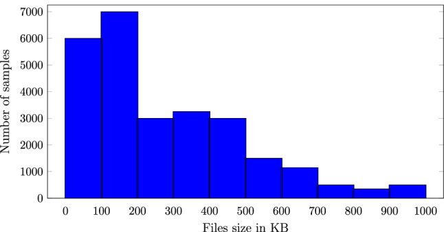
Histogram of MalExe file sizes

The average file size per family is given in Fig. 8. We observe that, for example, Lolyda has an average file size of 35KB, while the average file size of Adload is 602KB and Startpage has the largest average size at 1042KB.

Fig. 8.

MalExe average size per family

For our machine learning experiments, we need fixed-size input. There are multiple ways we can preprocess the data to achieve this. One reasonable approach is to extract a fixed amount of bytes and filter out smaller files, as is done in the papers [24, 32]. Another approach is to have variable sizes, then resize to the desired width and height. In Sect. 3.2, we discuss image extraction from executable files and we experiment with different file sizes, as well as grayscale and color images.

We divide this discussion of our implementation into four parts: dataset overview, image and feature extraction, data processing, and model hyperparameter tuning. We employ Google Colab Pro+ to utilize Google’s computing power to train multiple models on large datasets. Table 2 shows the runtime and memory settings for each model. Note that for XGBoost, we utilize GPUs for faster training time.

Table 2.

Runtime environment specifications

Models	Runtime	Memory
AC-GAN	TPU	35GB
DC-GAN	TPU	35GB
RBM	TPU	35GB
XGBoost	GPU	51GB
SVM	CPU	51GB
RF	CPU	51GB
KNN	CPU	51GB
MLP	CPU	51GB
Resnet152	TPU/CPU	35GB

Image extraction

The sizes of the executable files vary and, as mentioned above, we require fixed-size input for our learning experiments Here, we consider two distinct approaches to generate fixed-size images. Our first approach is based on resizing, while for the second, we simply truncate.

For our resizing approach, we first divide the samples into bins and set a corresponding image width per bin. For each bin, a fixed width and variable height is used based on the sizes given in [47]. Table 3 shows the details of the bins and width.

Table 3.

Image width based on file size

File size	Image width	File size	Image width
0KB–10KB	32	100KB–200KB	384
10KB–30KB	64	200KB–500KB	512
30KB–60KB	128	500KB–1000KB	768
60KB–100KB	256	$>$1000KB	1024

After generating images from executable files as described in the previous paragraph, we resize all images to $128\times 128$. We refer to this image-generation approach as our “resizing” method.

As an alternative approach for generating images from exe files, we simply truncate the malware samples to the desired size, with 0-paddings for smaller files. Thus, for $128\times 128$ images, we only use the first 16,384 bytes of each executable files. We refer to this image generation approach as the “truncating” method.

Grayscale images

Grayscale images are straightforward to generate from executable files—we simply interpret the bytes as pixels in an image. This is the most popular approach in the research literature for generating malware images; see, for example [24, 32, 52]. Only the byte sequence of the executable file is needed, and the processing is fast, even if resizing is employed. Examples of such grayscale malware images from our dataset are given in Fig. 9.

Fig. 9.

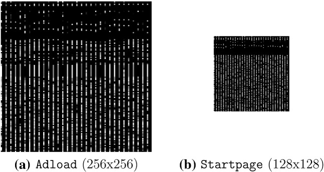
Examples of grayscale malware images

Color images using color map

In this section, we discuss generating color images from executable files using a color map, as in [43, 47]. First, we need to generate a 2D color map, which is a $16\times 16$ array where each element corresponds to an RGB value. There are a total 256 colors in this palette so we extract from the byte sequence a byte or 8-bit vector. We then split the byte into two parts, the first half of the byte represents the y-coordinate and the second half is the x-coordinate. We use these coordinates to obtain the RGB value from the color map. Specifically, we use the “plasma” colormap, as given in Fig. 10.

Fig. 10.

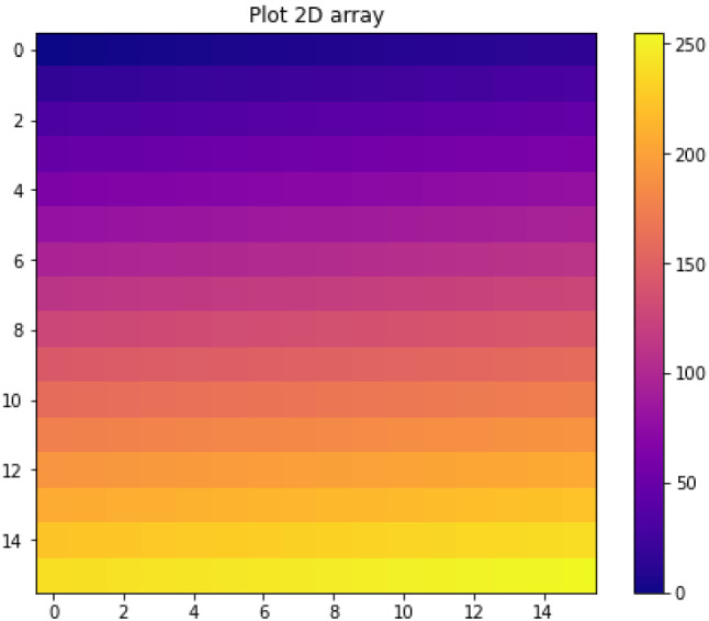
Plasma colormap

After we generate the images using the color map, the images have different sizes based on the file sizes. We then resize all images to the fixed $128\times 128$ as in the examples in Fig. 11. Each sample is now represented by an array of size $128\times 128\times 3$, and the data is ready to feed into machine learning models for training. We refer to this method as the “colormap” method.

Fig. 11.

Colormap images of different families

Color images using three consecutive bytes

Another method for generating color images that we consider is to let three consecutive byte values correspond to the R, G and B layers of an RGB image. We found that, visually, the resulting images were not as colorful as expected. Therefore, we kept the red and green layers, but replaced the blue value with

$$\begin{array}{c}\hfill \text{blue}=255-\text{ByteValue}.\end{array}$$

The resulting three-grams images tend to have a blue background so that we can more easily distinguish them from grayscale images. Examples of this type of malware-derived color image are given in Fig. 12. We refer to this method of generating color images as the “three-gram” approach.

Fig. 12.

Three-gram images of different families

Next, we discuss our fourth method for generating images Then we conclude this section with a discussion of data pre-processing and model hyperparameter tuning.

Color images from the PE file format

Fu et al. [16] proposed to transform malware executables into color images based on the Windows PE file format. For each PE section, the entropy value is calculated once and used as the R layer for the whole section. The B layer is represented using the relative size of a section, while the G layer is just the byte values (as in grayscale images). We experimented with this method to extract colorful images from malware files. Entropy values and size ratios are calculated and scaled to the range of 0 to 255. The formulas for red and blue layers are

$$\begin{array}{c}\hfill \text{RedLayer}=\text{Entropy}\times \frac{255}{8}\text{and}\text{BlueLayer}=\frac{\text{SectionSize}}{\text{FileSize}}\times 255.\end{array}$$

Figure 13 shows the PE images of samples from three families, namely, Adload, Startpage, and Ceeinject. Note that Ceeinject uses extensive obfuscation, so we expect images from the Ceeinject family to differ more significantly than samples in the Adload or Startpage families

Fig. 13.

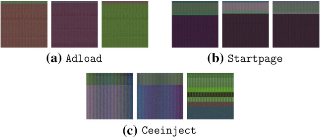
PE images of different families

Data processing

GANs require input data in the form of a 3-dimension array, while many other techniques (e.g., SVM and XGBoost) expect 1-dimension array input. Therefore, we convert images to vectors by flattening and scaling according to

$$\begin{array}{c}\hfill \overline{x}=\frac{x-\mu }{\sigma }\end{array}$$

where $\mu$ is the mean and $\sigma$ is the standard deviation. Data that is scaled to be between 0 and 1 may result in faster and more stable computation in XGBoost and RBM experiments.

Experiments and results

In this section, we present and analyze our experimental results. First, we consider model hyperparameter tuning. This is followed by extensive multiclass experiments, where we compare a wide variety of classification techniques, and we test each of the four image generation methods introduced in Sect. 3.2, above. For our final set of experiments, we analyze the generative capabilities of GAN-based techniques.

Model hyperparameter tuning

Figures 24 and 25 in the Appendix show the AC-GAN generator and discriminator architectures, respectively. Note that these architectures are specific to color images of size $128\times 128$, and that they are the same as those used in [7]. For other images, minor modifications are required

Fig. 24.

AC-GAN generator architecture

Fig. 25.

AC-GAN discriminator architecture

For the AC-GAN generator, Manisha et al. [36] showed that for color images with sizes of $64\times 64$ and above, increasing the noise dimension has a significant positive impact on the generative images, and therefore both the discriminator and generator models would benefit. For this reason, we choose the noise dimension vectors for the generator to be size (1000, 1) instead of the more typical (100, 1) for images of size $28\times 28$ [36].

We perform hyperparameter tuning on each of our models using a grid search. The hyperparameters tested and selected for our RF, k-NN, MLP, SVM, and XGBoost models are given in Tables 4 (a) through (e), respectively, where in each case, the selected best hyperparameter value is in boldface. For example, for RF, we found that 600 estimators, the entropy function, and a maximum depth of 6 yielded the best results.

Table 4.

Hyperparameters tested and selected

Parameters	Description	Tested
(a) Random forest hyperparameters
nestimators	Number of estimators	100,200,400,600
criterion	Function to measure quality	gini, entropy
maxdepth	Maximum depth	3,4,5,6
(b) k-NN hyperparameters
nneighbors	Number of neighbors	5,10,20,40
weights	Function used in prediction	uniform, distance
(c) MLP hyperparameters
hiddenlayer	Sizes	(100,100,20), (100,100,100,20)
activation	Activation function	logistic, tanh, relu
alpha	L2 penalty	0.0001, 0.001, 0.01
(d) SVM hyperparameters
kernel	Kernel function	rbf, linear, poly
C	Regularization parameter	1,10,100
(e) XGB hyperparameters
maxdepth	Maximum depth	4,5,6,7
learningrate	Learning rate	0.01, 0.02, 0.03
nestimators	Number of estimators	200,400,600

Multiclass classification

We compare the performance of AC-GAN, RBM, SVM, and XGBoost on the four image extraction methods discussed above. Then we select the best of these image extraction method to compare GANs with other popular machine learning models. This latter comparison is with respect to a challenging multiclass malware classification problem.

Image extraction comparison

Figure 14 provides our results for each of the four image extraction techniques considered—grayscale, colormap, PE, and three-gram—using each of the classifiers AC-GAN, RBM, SVM, and XGBoost. We observe that the PE features perform the worst, while the color three-grams sightly outperform grayscale images, with the truncated colormap approach being the best overall. XGBoost, outperforms the other learning techniques in all cases, but we will conduct a much more thorough comparison of learning techniques in the next section.

Fig. 14.

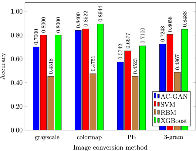
Accuracies for malware families classification

In summary, we have determined that the truncated colormap method provides the best performance among the image generation techniques tested. In the next section, we compare a wide variety of learning techniques based on this truncated colormap method. For the colormap experiments in the next section, we only consider the first $128\times 128$ bytes of the executables; if the file size is smaller, we pad with 0 to the necessary size.

Machine learning model comparison

Figure 15 shows the accuracy and loss graphs for both training and testing of the AC-GAN discriminator. After 30 epochs, there is no significant improvement in the discriminator, and therefore in all subsequent experiments, we train the AC-GAN discriminator for 30 epochs.

Fig. 15.

AC-GAN discriminator loss and accuracy

Malware classification results for all of the classifiers we tested are given in Table 5. From this table, we see that Resnet152 performs the best, with XGBoost, MLP, and AC-GAN all yielding reasonably strong results.

Table 5.

Results of various models on truncated colormap images

Models	Type	Accuracy	Precision	Recall	F1-Score
k-NN	Maching learning	76.94%	87%	77%	79%
SVM	Machine learning	85.22%	88%	86%	86%
MLP	Machine learning	86.97%	86%	86%	86%
RF	Ensemble	72.56%	80%	69%	70%
XGBoost	Ensemble	89.44%	90%	89%	89%
AC-GAN	Deep learning	84.00%	86%	86%	85%
Resnet152	Deep residual network	91.39%	91%	91%	91%

Figure 16 compares the training time and performance of the various models. MLP and XGBoost perform exceptionally well considering the training time is less than some of the other deep learning models, such as AC-GAN. Resnet152 is clearly our best model, as it gives the best performance, and the training time is fast due to it being pre-trained. AC-GAN takes approximately 500 seconds per epoch, or around 4 hours to finish training; SVM takes 3 hours for training and 2 hours for prediction. All of our other models are relatively fast, with each taking less than an hour to train.

Fig. 16.

Accuracy versus training time

As ResNet152 is our best performer, we provide its confusion matrix in Fig. 17. We can see that the three families that are causing the most classification problems for this model are Obfuscator, Rbot, and Agent. Since Obfuscator obfuscates its code, we expect this family to be a difficult classification problem. Agent is a general family that includes malware with multiple purposes, and it also makes sense that machine learning models would have difficulty classifying more general types.

Fig. 17.

Confusion matrix for Resnet152 using colormap method

Figure 18 confirms that more general and heavily obfuscated families are hard to classify. These families include Agent, Ceeinject, Obfuscator, and Rbot, which are consistently classified poorly by all learning techniques tested. Resnet152 performs best on most of the families. Interestingly, although k-NN does not perform well overall, it performs better than any of the other models on the challenging Agent family.

Fig. 18.

F1 scores for each family

Ensemble classifiers

In an attempt to improve the accuracy for the most difficult families, such as Agent or Rbot, we generate an ensemble based on all 7 of the classifiers discussed above: AC-GAN, k-NN, MLP, Resnet152, RF, SVM, and XGBoost. First, we consider a simple voting procedure, where the family with the most votes from among the 7 classifiers is selected—in case of a tie, we select randomly from those families with the most votes. This voting ensemble yields an accuracy of 91.60%, which is only a marginal improvement over the 91.39% accuracy achieved by ResNet152 alone.

As a second ensemble experiment, we generate feature vectors using the 7 models and train another classifier. AC-GAN and Resnet152 produce $20\times 1$ output vectors, while all other models generate one class label. These feature vectors are concatenated and used to train a Random Forest (RF) model. This RF based ensemble yields an accuracy of 92.09%. Interestingly, this RF model provides a noticeable improvement on the more difficult families, although it performs somewhat worse than Resnet152 on the easier families, including Cycbot, Adload, and Alureon. We provide the confusion matrix for this model in Fig. 19. Apparently, the “noise” from the other other models causes the RF classifier to make more mistakes than Resnet152 on the easier models.

Fig. 19.

Confusion matrix for Random Forest ensemble

GAN generated images

Recall that DC-GAN is an unsupervised architecture, which implies that we do not directly obtain accuracy scores from a DC-GAN discriminator model. However, we can use DC-GAN to analyze the generative power of our AC-GAN generators. Figure 20 shows a comparison between real and generated images using DC-GAN. Although not perfect replicas, the DC-GAN images do appear to capture some significant characteristics of the real images.

Fig. 20.

Real versus fake images (DC-GAN and Adload family)

Recall that AC-GAN is a multiclass GAN, and hence it uses class labels when generating images. Figures 21 and 22 show real and AC-GAN generated images from the Ceeinject and Adload family, respectively. In the case of AC-GAN, these “deep fake” images appear to be excellent representations of the real malware images.

Fig. 21.

Real and fake images of Ceeinject family

Fig. 22.

Real and fake color images of Adload family

To analyze the performance of our generator, below we experiment with binary classification, i.e., malware versus benign. We use a dataset of 704 benign executables, extract images from them using the Colormap method then use SVM, RF, and CNN to determine how well we can distinguish these benign samples from a random selection of malware samples. Finally, we mix the benign samples with fake malware images from AC-GAN and compare the detection performance. This latter experiment simulates an adversarial attack, where GAN-generated images are used to corrupt the training data of a model.

Binary classification results

For our first set of binary classification experiments, our dataset consists of 10,000 malware samples from 20 families (approximately 500 samples per family) and 704 benign samples. We use colormap images and SVM for these malware detection experiment. We find that the 5-fold cross validation results range from 99% to 100%, both in terms of accuracy and AUC.

Next, we train models to distinguish between 10,000 fake malware images and 10,000 real malware images. Here, we ignore the benign set and we are simply trying to distinguish between real and fake images. In this case, both SVM and RF models score 99% to 100% in accuracy and AUC. This shows that GAN-generated images are surprisingly easy to distinguish from real images. Since the fake images are easily distinguished from real, we can use a 2-level detection strategy, where we first filter out the malware corresponding to fake images, and then classify the remaining samples by any strategy that we prefer. This shows that our GAN-generated malware images cannot be used effectively in an adversarial attack on the image-based malware classifiers that we have considered.

In addition to AC-GAN and DC-GAN, we experimented with Wasserstein GANs with gradient penalty (WGAN-GP). As WGAN-GP requires intensive computation power and training time, we only trained for 100 epochs, whereas 300 epochs were used for DC-GAN. As with the AC-GAN and DC-GAN images, we are still able to distinguish the WGAN-GP images from real malware images with 99% to 100% accuracy and AUC for both SVM and RF classifiers. We experiment with the three-gram method using AC-GAN, and obtained similar results.

Discussion

Intuitively, since a GAN model includes a generator and a discriminator, it should improve both models, as compared to other approaches. In our experiments, we found that an AC-GAN discriminator performs well when trained for 30 epochs, while the AC-GAN generator requires at least 200 epochs to produce visually impressive images. Figure 23 shows a comparison between a real image and generated images after 30 epochs and 200 epochs. At 200 epochs, the AC-GAN generator clearly performs better. However, the AC-GAN discriminator shows definite signs of overfitting at such a high number of epochs, with its accuracy decreasing to 65%.

Fig. 23.

Real and fake color images of Adload family

As with our multiclass malware family experiments, Resnet152 outperforms AC-GAN in our malware detection (i.e., binary classification) experiments. Resnet152 also has a substantially faster training time. This again shows an advantage of a pre-trained model, and indicates that image-based malware classification should generally emphasize pre-trained models, such as Resnet152 and VGG19. Nevertheless, it is interesting that the AC-GAN classifier is highly competitive for malware detection, and it is somewhat surprising that visually impressive GAN-generated images are so easily distinguished from real malware samples.

Conclusion and future works

We experimented with four different ways of extracting images from malware executables: grayscale, colormap, three-gram, and PE. We found that based on the same amount of data, the colormap method improves the overall results for all models, with AC-GAN showing the most improvement for the malware families classification problem. XGBoost and RBM were faster to train as compared to SVM or GAN; however for XGBoost the memory requirement is high.

As expected, our models do not do as well with malware families that are more general or obfuscated. For future work, experiments with transformers or Long Short-Term Memory (LSTM) would be worth considering, especially with respect to the more highly obfuscated malware families. The PE image method did not perform well in our experiments, but we believe that this image generation method has considerable room for improvement. Other image generation methods could also be considered. In particular, it might be advantageous to consider images with a depth of two which has a more natural interpretation in terms of exe files. In our experiments, we chose a depth of three, simply in analogy to RGB colors.

There are many GAN variants (StyleGAN, MalGAN, etc.) that could be considered, especially with respect to the malware image generation problem. Designing a new GAN architecture or changing the AC-GAN loss function to speed up the training process of its generator would also be interesting topics to explore.

Our GAN-generated images do not directly correspond to functioning malware samples, which maximized our freedom to generate high quality images. Nevertheless, we showed that the resulting GAN images are easily distinguished from real malware images using an SVM or Random Forest. To generate GAN images that are easily converted to functioning malware is challenging future work. This would likely place considerably more constraints on the GAN itself and, ironically, would likely make the samples even easier to distinguish from benign samples.

Appendix

In this appendix, we provide details of the AC-GAN generator and discriminator architectures (Figs. 24 and 25). Note that these architectures are specified to the case of color images of size $128\times 128$. Other images and sizes are straightforward modifications.

Declarations

Conflicts of interest

The authors have no relevant financial or non-financial interests to disclose.