spsurvey: Spatial Sampling Design and Analysis in R

Abstract

spsurvey is an R package for design-based statistical inference, with a focus on spatial data. spsurvey provides the generalized random-tessellation stratified (GRTS) algorithm to select spatially balanced samples via the grts() function. The grts() function flexibly accommodates several sampling design features, including stratification, varying inclusion probabilities, legacy (or historical) sites, minimum distances between sites, and two options for replacement sites. spsurvey also provides a suite of data analysis options, including categorical variable analysis (cat_analysis()), continuous variable analysis cont_analysis()), relative risk analysis (relrisk_analysis()), attributable risk analysis (attrisk_analysis()), difference in risk analysis (diffrisk_analysis()), change analysis (change_analysis()), and trend analysis (trend_analysis()). In this manuscript, we first provide background for the GRTS algorithm and the analysis approaches and then show how to implement them in spsurvey. We find that the spatially balanced GRTS algorithm yields more precise parameter estimates than simple random sampling, which ignores spatial information.

1. Introduction

Survey designs are often used to study an environmental resource in a population. These populations are comprised of individual population units, which are often referred to as sites. Each site contains information about the environmental resource, and a complete characterization of the resource can be obtained by studying every site. Unfortunately, studying every site is rarely feasible. Therefore, a sample of sites is collected, and the sample is used to make generalizations about the larger population. Typically sites are selected without replacement, and we make this assumption henceforth. The process by which sites are selected in the sample is known as the sampling design.

In the design-based approach to statistical inference, a sample should be representative of the population, but the term representative is often vague and has multiple interpretations (Kruskal and Mosteller 1979a,b,c). We claim a representative sample should have at least the following two properties. First, the sites must be selected as part of the sample via a random mechanism. The design-based approach to statistical inference relies on a random selection of sites; the random site selection forms the foundation for deriving properties of parameter estimates (Särndal, Swensson, and Wretman 2003; Lohr 2009). Second, the probability each site is selected as part of the sample is greater than zero. This probability of selection is known as an inclusion probability.

There are three types of commonly studied environmental resources: point resources, linear resources, and areal resources. A point resource has a finite number of population units (i.e., a finite population) and represents a collection of point geometries. An example of a point resource is all lakes (viewed as a whole) in the United States, using the centroid of the lake as the site location. A linear resource has an infinite number of population units (i.e., an infinite population) and represents a collection of linestring geometries. An example of a linear resource is all streams in the United States. An areal resource has an infinite number of population units and represents a collection of polygon geometries. An example of an areal resource is the San Francisco Bay Estuary.

These point, linear, and areal resources tend to be spread over geographic space. If a sample is well-spread over geographic space, we call it a spatially balanced sample (we provide a more technical definition of spatial balance in Section 2.2). Spatially balanced samples are desirable because they tend to yield more precise parameter estimates than samples that are not spatially balanced (Stevens and Olsen 2004; Barabesi and Franceschi 2011; Grafström and Lundström 2013; Robertson, Brown, McDonald, and Jaksons 2013; Wang et al. 2013; Benedetti, Piersimoni, and Postiglione 2017).

The spsurvey package (Dumelle, Kincaid, Olsen, and Weber 2023) selects spatially balanced samples using the generalized random-tessellation stratified (GRTS) algorithm (Stevens and Olsen 2004) and is available from the Comprehensive R Archive Network (CRAN) at https://CRAN.R-project.org/package=spsurvey. Shortly after the GRTS algorithm emerged, several other spatially balanced sampling algorithms followed. Walvoort, Brus, and De Gruijter (2010) used compact geographical strata to perform stratified sampling; this approach is available in the spcosa R package (Walvoort, Brus, and De Gruijter 2022). Grafström, Lundström, and Schelin (2012) used a local pivot method for finite populations and Grafström and Matei (2018) generalized this approach to infinite populations; these approaches are available in the BalancedSampling R package (Grafström and Lisic 2019). Grafström (2012) used a spatially correlated Poisson approach, also available in BalancedSampling. Benedetti and Piersimoni (2017) used a within-sample distance approach available in the Spbsampling R package (Pantalone, Benedetti, and Piersimoni 2022). Robertson et al. (2013) developed balanced acceptance sampling, and subsequently, Robertson, McDonald, Price, and Brown (2018) used Halton iterative partitioning; these approaches are available in the SDraw R package (McDonald and McDonald 2020). Foster et al. (2020) developed spatially balanced transect sampling; this approach is available in the MBHdesign R package (Foster 2021).

The GRTS algorithm in spsurvey implements many features absent from the aforementioned software packages. The GRTS algorithm in spsurvey can be applied to all three resource types: point, linear, and areal. It accommodates several sampling design features like stratification, unequal selection probabilities, legacy (or historical) sites, minimum distances between sites, and two options for replacement sites (reverse hierarchical ordering and nearest neighbor). The GRTS algorithm is discussed in more detail in Section 2. Section 2 also showcases how spsurvey can be used to summarize and visualize sampling frames and samples as well as measure spatial balance.

Another benefit of spsurvey compared to the aforementioned software packages is that spsurvey can also be used to analyze data and estimate parameters of a population. spsurvey has a suite of analysis functions that enable categorical variable analysis, continuous variable analysis, attributable risk analysis, relative risk analysis, difference in risk analysis, change analysis, and trend analysis. In addition, variances can be estimated using the local neighborhood variance estimator (Stevens and Olsen 2003), which increases precision by using the spatial locations of each observation in variance estimation. The analysis functions in spsurvey are discussed in more detail in Section 3.

The rest of this paper is organized as follows. In Section 2, we review spatially balanced sampling in spsurvey. In Section 3, we the describe the analysis approaches available in spsurvey. In Section 4, we compare performance of the GRTS algorithm and local neighborhood variance estimator to simple random sampling using data from the 2012 National Lakes Assessment (U.S. Environmental Protection Agency 2017). Finally, in Section 5, we end with a discussion and explore potential future developments for spsurvey.

To install and load spsurvey, run

R> install.packages(“spsurvey”) 
R> library(“spsurvey”)

2. Spatially balanced sampling

In Section 1 we introduced the notion of a random sample. Random samples are selected from a collection of sites. This collection of sites is known as the sampling frame. Ideally, the set of sites in the sampling frame is the same as the set of sites in the population. Unfortunately this is not always true, as a sampling frame may contain some sites that are not in the population (overcoverage), may be missing sites from the population (undercoverage), or both. Selecting an appropriate sampling frame is crucial if you want to generalize results from the sample to the population. To understand whether a sampling frame is appropriate for a population, summaries and visualizations of the sampling frame are helpful. Next we demonstrate using spsurvey to summarize and visualize sampling frames. We then give theoretical background for the generalized random-tessellation stratified (GRTS) algorithm and show how to use it in spsurvey to select spatially balanced samples and to summarize, visualize, write, and print these samples. We end the section by showing how to explicitly measure spatial balance using spsurvey and to use GRTS for a variety of resource types.

2.1. Summarizing and visualizing sampling frames

Sampling frames for point, linear, or areal resources summarized and visualized in spsurvey using the summary() and plot() functions, respectively. The summary() and plot() functions have similar syntax and require at least two arguments: the sampling frame and a formula. The sampling frame must be an ‘sf’ object (Pebesma 2018) or a data frame. The formula specifies the variables in the sampling frame to summarize or visualize and can be one-sided or two-sided. Additional arguments to summary() and plot() are discussed in more detail later.

To demonstrate the use of summary() and plot(), we use the the NE_Lakes data in spsurvey. The NE_Lakes data is an ‘sf’ object of 195 lakes in the Northeastern United States. The NE_Lakes data represent a point resource, as there are a finite number of lakes to sample. Later we study linear and areal data in spsurvey. To load NE_Lakes into your global environment, run

R> data(“NE_Lakes”, package = “spsurvey”)

There are five variables in NE_Lakes: AREA, a continuous variable representing lake area (in hectares); AREA_CAT, a categorical variable representing lake area levels small (1 to 10 hectares) and large (greater than 10 hectares); ELEV, a continuous variable representing lake elevation (in meters); and ELEV_CAT, a categorical variable representing lake elevation levels low (0 to 100 meters) and high (greater than 100 meters). We can view the geometry information and first few rows of NE_Lakes by running

R> NE_Lakes

Simple feature collection with 195 features and 4 fields
Geometry type: POINT
Dimension:     XY
Bounding box:  xmin: 1834001 ymin: 2225021 xmax: 2127632 ymax: 2449985
Projected CRS: NAD83 / Conus Albers 
First 10 features:

	AREA	AREA_CAT	ELEV	ELEV_CAT	geometry
1	10.648825	large	264.69	high	POINT (1930929 2417191)
2	2.504606	small	557.63	high	POINT (1849399 2375085)
3	3.979199	small	28.79	low	POINT (2017323 2393723)
4	1.645657	small	212.60	high	POINT (1874135 2313865)
5	7.489052	small	239.67	high	POINT (1922712 2392868)
6	86.533725	large	195.37	high	POINT (1977163 2350744)
7	1.926996	small	158.96	high	POINT (1852292 2257784)
8	6.514217	small	29.26	low	POINT (1874421 2247388)
9	3.100221	small	204.62	high	POINT (1933352 2368181)
10	1.868094	small	78.77	low	POINT (1892582 2364213)

Notice that the geometry type of NE_Lakes is POINT, as NE_Lakes represents a point resource.

Before summarizing or visualizing NE_Lakes, store it as an ‘sp_frame’ object by running

R> NE_Lakes <- sp_frame(NE_Lakes)

One-sided formulas are used when the goal is to summarize or visualize variables individually. To summarize the distribution of ELEV_CAT using a one-sided formula, run

R> summary(NE_Lakes, formula = ~ ELEV_CAT) 

total	ELEV_CAT
total:195	low :112
	high: 83

The output contains two columns: total and ELEV_CAT. The total column acts as an “intercept” in the formula and returns the total number of observations in the sampling frame; it can be omitted by supplying - 1 to the formula. The ELEV_CAT column returns the number of lakes in the low and high elevation levels. The same syntax is used to visualize the spatial distribution of ELEV_CAT (Figure 1a):

Figure 1:

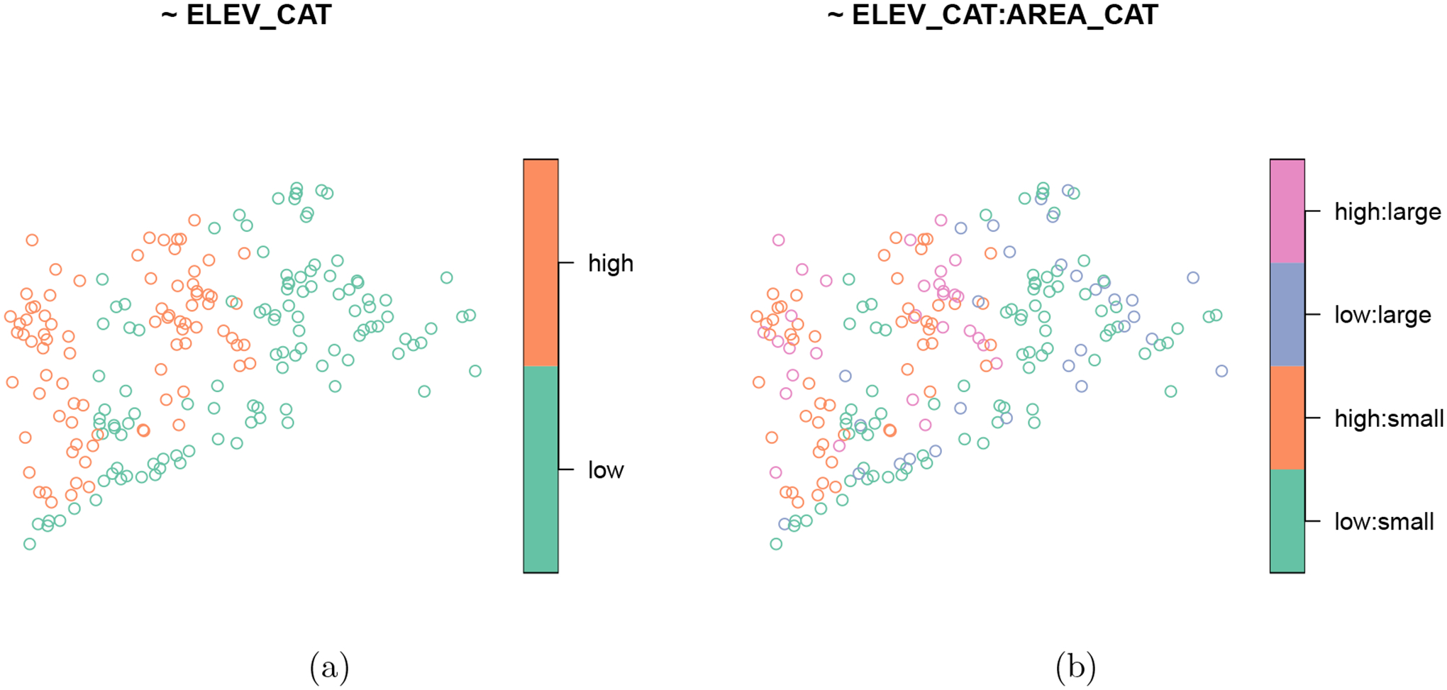
Distribution of the lake elevation categories (a) and the interaction between lake elevation categories and lake area categories (b) in the Northeastern lakes data.

R> plot(NE_Lakes, formula = ~ ELEV_CAT)

By default, the formula argument to plot() is the resulting plot’s title, though this can be changed using the main argument.

Additional variables can be added to the formula when separated by +. Interactions between variables can be added to the formula using :. When additional variables are added, summary() produces a table-like summary of each variable

R> summary(NE_Lakes, formula = ~ ELEV_CAT + ELEV_CAT:AREA_CAT)

total	ELEV_CAT	ELEV_CAT:AREA_CAT
total:195	low :112	low:small :82
	high: 83	high:small:53
		low:large :30
		high:large:30

Similarly, plot() produces separate visualizations for each variable (Figure 1).

R> plot(NE_Lakes, formula = ~ ELEV_CAT + ELEV_CAT:AREA_CAT)

These separate visualizations are stepped through using <Return>. The summary() and plot() functions also support standard formula syntax shortcuts like . and *. The formula ~ . is shorthand for ~ AREA + AREA_CAT + ELEV + ELEV_CAT and the formula ~ AREA_CAT * ELEV_CAT is shorthand for ~ AREA_CAT + ELEV_CAT + AREA_CAT : ELEV_CAT.

Two-sided formulas are useful when the goal is to summarize or visualize one variable (a left-hand side variable) for each level of other variables (right-hand side variables). When using two-sided formulas, summary() returns table-like summaries of the left-hand side variable for each level of each right-hand side variable:

R> summary(NE_Lakes, formula = ELEV ~ AREA_CAT)

ELEV by total:
	Min.	1st Qu.	Median	Mean	3rd Qu.	Max.
total	0	21.925	69.09	127.3862	203.255	561.41

ELEV by AREA_CAT:
	Min.	1st Qu.	Median	Mean	3rd Qu.	Max.
small	0.00	19.64	59.660	117.4473	176.1700	561.41
large	0.01	26.75	102.415	149.7487	241.2025	537.84

plot() returns separate visualizations of the left-hand side variable for each level of each right-hand side variable. For example,

R> plot(NE_Lakes, formula = ELEV ~ AREA_CAT)

produces two separate visualizations – one for each level of AREA_CAT (small and large).

The plot() function has additional arguments that allow for flexible customization of graphical parameters. The varlevel_args (short for “variable level arguments”) argument adjusts graphical parameters separately for each level of a categorical variable. The var_args (short for “variable arguments”) argument adjusts graphical parameters for a numeric variable or simultaneously for all levels of a categorical variable. The … argument adjusts graphical parameters for all variables simultaneously. spsurvey’s plot() function is built on top of sf’s plot() function. As a result, it takes the same set of graphical parameters that sf’s plot() function does and uses the same default values.

2.2. The generalized random-tessellation stratified algorithm

Before discussing the GRTS algorithm, it is important to identify two distinct types of spatial balance: spatial balance with respect to the sampling frame and spatial balance with respect to geography. Spatial balance with respect to the sampling frame measures how closely the spatial layout of the sample resembles the spatial layout of the sampling frame. Spatial balance with respect to geography measures the geographic spread of the sample – usually the sites in the sample are spread out over the domain in some equidistant manner but are not meant to resemble the spatial layout of the sampling frame. While spatial balance with respect to geography can be useful, spatial balance with respect to the sampling frame is preferred for design-based inference because this type of spatial balance is closely linked to inclusion probabilities, which we discuss in more detail later. Henceforth, when we refer to spatial balance, we mean spatial balance with respect to the sampling frame.

Stevens and Olsen (2004) created the first widely-used spatially balanced sampling algorithm known as the GRTS algorithm. The GRTS algorithm has several attractive properties we discuss throughout this subsection. Most notably, the GRTS algorithm accommodates all three resource types: point, linear, and areal. It also accommodates a suite of flexible sampling design options like stratification, unequal inclusion probabilities, legacy (historical) sites, a minimum distance between sites, and two options for replacement sites. Next we provide a brief overview of the technical details of the algorithm as described by Stevens and Olsen (2004).

The first step in the GRTS algorithm is to determine the probability that each site is selected in the sample, known as an inclusion probability. For example, if the population size N equals 100, the sample size n equals 10, and each site is equally likely to be selected in the sample, then each site’s inclusion probability is n/N = 10/100 = 0.1. After determining these inclusion probabilities, a square bounding box is superimposed onto the sampling frame. That bounding box is divided into four distinct, equally sized square cells. These cells compose the first level of a hierarchical grid and are called level-one cells. These level-one cells are randomly assigned a level-one address of zero, one, two, or three. The set of level-one cells is denoted by 𝒜₁ and defined as 𝒜₁ ≡ {a₁ : a₁ = 0,1,2,3} (Figure 2a). Each level-one cell has an inclusion value that equals the sum of the inclusion probabilities for the sites contained in the level-one cell. If any of the level-one cell’s inclusion values are larger than one, a second level of cells is added by splitting each level-one cell into four distinct, equally sized squares. Together these small squares compose the second level of a hierarchical grid and are called level-two cells. Within each level-one cell, the level-two cells are randomly assigned a level-two address of zero, one, two, or three. The level-one and level-two addresses compose a set that can be used to identify any level-two cell. The set of level-two cells is denoted by 𝒜₂ and defined as 𝒜₂ ≡ {a₁a₂ : a₁ = 0,1,2,3;a₂ = 0,1,2,3} (Figure 2b). If any of the level-two cell’s inclusion values are greater than one, a third level of cells is added. This process continues for k levels, where k is the first level that all level-k cells have inclusion values no greater than one. Then 𝒜_k ≡ {a₁ …a_k : a₁ = 0,1,2,3;…;a_k = 0,1,2,3}. This addressing composes a base-four ordering scheme – Stevens and Olsen (2004) provide further details.

Figure 2:

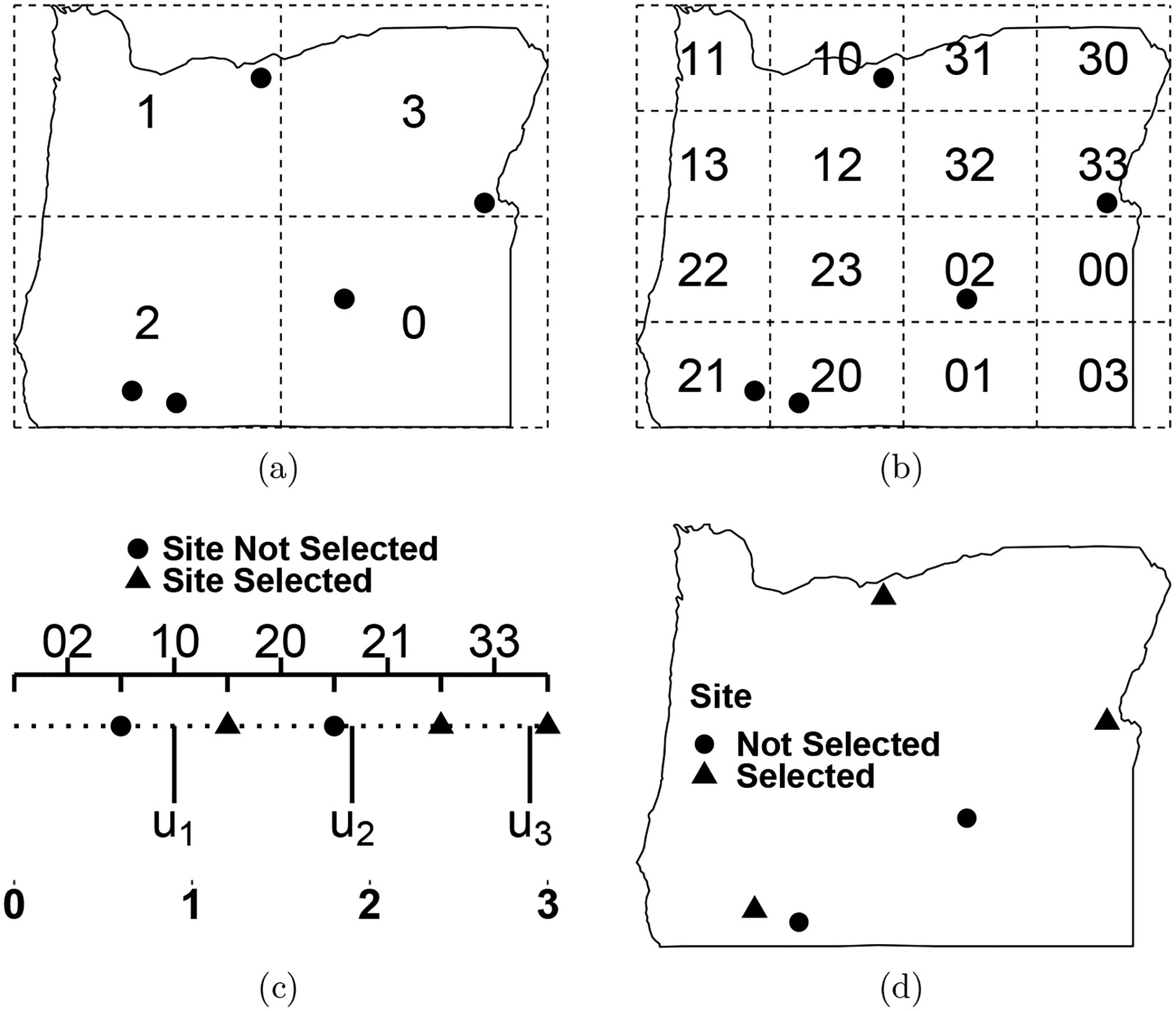
A visual description of the generalized random-tessellation stratified algorithm using sites from an illustrative sampling frame in Oregon, USA. In (a), the level-one cells are superimposed onto the sampling frame. In (b), the level-two cells are superimposed onto the sampling frame. In (c), the level-two cells are mapped in heirarchical order from two-dimensional space to a line and a sample is selected. Each cell is represented by brackets with a closed right endpoint, meaning they contain the site at their closed right boundary. In (d), the sites are separated by whether or not they are part of the sample.

Next the elements in 𝒜_k are placed in hierarchical order. Hierarchical order is a numeric order that first sorts 𝒜_k by the level-one addresses from smallest to largest, then by the level-two addresses from smallest to largest, and so on. For example, 𝒜₂ in hierarchical order is the set {00,01,02,03,10,…,13,20,…,23,30,…,33}. Then the level-k grid cells are mapped from two-dimensional space to a line in hierarchical order (Figure 2c). More specifically, mapping a level-k grid cell means placing each site in the level-k grid cell on the line, where each site is represented by a line segment with length equal to its inclusion probability. The hierarchical ordering tends to map nearby sites in two-dimensional space to nearby locations on the line. Because the entire line represents the inclusion probabilities of each site, the line’s total length equals the sum of these inclusion probabilities. This sum equals n, the desired sample size.

After hierarchically ordering the sites and placing them on the line, the sample is selected. To select a sample, Stevens and Olsen (2004) denote a uniform random variable simulated from [0,1] as u₁ and place it on the line. The location of u₁ on the line corresponds falls within some line segment that represents a site, which we denote s₁. The site s₁ is then the first site selected as part of the sample. Next we define u₂ ≡ u₁ + 1, which falls within a line segment that represents another site, which we denote s₂. The sites s₁ and s₂ must be distinct because of the requirement that each level-k cell has inclusion value no greater than one. Then u₃ ≡ u₂ + 1 corresponds to s₃ and so on until the set {u₁,…,u_n} corresponds to the set {s₁,…,s_n}, which are the n sites included in the sample (Figure 2d). Stevens and Olsen (2004) provide further details.

spsurvey implements the GRTS algorithm using the grts() function. There are two required arguments to grts(): the sampling frame and a base sample size. The first required argument is the sampling frame, which must be an ‘sf’ object. For point resources, the sf geometries must all be POINT or MULTIPOINT; for linear resources, the sf geometries must all be LINESTRING or MULTILINESTRING; and for areal resources, the sf geometries must all be POLYGON or MULTIPOLYGON. The second required argument is the desired sample size for the base sample, n_base. The base sample is a sample that does not include replacement sites (Section 2.2.3). Additional arguments to the grts() function address specific sampling design options, which we discuss later.

The output from the grts() function is a list five components: sites_legacy, sites_base, sites_over, sites_near, and design. sites_legacy, sites_base, sites_over, sites_near are ‘sf’ objects containing the legacy sites (discussed in Section 2.2.1), base sites (except for those already included in sites_legacy), replacement sites using reverse hierarchical ordering (Section 2.2.3), and replacement sites using nearest neighbor (Section 2.2.3), respectively. Together, the collection of these sites objects are called the design sites. Each sites object contains all original columns from the sampling frame and some additional columns related to the sampling design. The last component of the grts() function output is a list named design, which contains details regarding the sampling design. Next we give some examples implementing the grts() function.

To select a GRTS sample of size 50 where each site has an equal inclusion probability, run

R> eqprob <- grts(NE_Lakes, n_base = 50)

Instead of sampling from the entire sampling frame simultaneously, it is common to divide a sampling frame into distinct sets of sites known as strata and select samples from each stratum independently of other strata. This approach is known as stratification and yields a stratified sample. Särndal et al. (2003) mentions several practical and statistical benefits of stratified samples compared to unstratified samples. One such practical benefit is that stratification allows for stratum-specific sample sizes and implementation practices (e.g., each stratum may have different sampling protocols). One such statistical benefit is that stratification tends to increase precision of parameter estimates. To select a GRTS sample stratified by the lake elevation categories where all sites within a stratum have equal inclusion probabilities, run

R> n_strata <- c(low = 35, high = 15)
R> eqprob_strat <- grts(NE_Lakes, n_base = n_strata,
+    stratum_var = “ELEV_CAT”)

In a stratified sample, n_base must be a named vector whose names (low and high) represent each stratum and whose values represent stratum-specific sample sizes (35 and 15). stratum_var is the name of the column in the sampling frame that represents the stratification variable.

Sometimes the desire is to sample sites that belong to some level of a categorical variable more often than others levels. For example, suppose large lakes are to be sampled more often than small lakes. To select a GRTS sample with unequal inclusion probabilities based on lake area categories, run

R> caty_n <- c(small = 10, large = 40)
R> uneqprob <- grts(NE_Lakes, n_base = 50, caty_n = caty_n,
+    caty_var = “AREA_CAT”)

caty_n is a named vector whose names represent the categorical area levels (small and large) and whose values represent the expected within-level sample sizes. caty_var is the name of the column in the sampling frame that represents the unequal probability variable. If the sample is stratified, caty_n must instead be a list whose names match the names of n_base and whose values are named vectors. Each named vector has names that represent the categorical variable levels and values that represent within-strata expected sample sizes.

Another approach is to sample sites proportionally to a positive auxiliary variable, which is sometimes referred to as proportional to size (PPS) sampling. PPS sampling can yield more efficient estimators when the response and auxiliary variables are positively correlated Särndal et al. (2003). To select a GRTS sample with inclusion probabilities proportional to lake area, run

R> propprob <- grts(NE_Lakes, n_base = 50, aux_var = “AREA”)

aux_var is the name of the column in the sampling frame that represents the PPS auxiliary variable.

Legacy sites

Often it is desired that some sites selected from an old sample are guaranteed to be selected in a new sample. Foster et al. (2017) discusses two types of sites that can be used to accomplish this goal: legacy (historical) sites and iconic sites. Legacy sites were randomly selected in the old sample, are in the current sampling frame, and must be in the current sample. Together, this implies that the new sample can be viewed as a possible joint realization from solely the current sampling frame. Legacy sites are often used to study behavior through time and can beneficial to estimation Urquhart and Kincaid (1999). Iconic sites, however, are not required to be randomly selected in the old sample or to be contained in the current sampling frame. Iconic sites are typically used because they represent sites of particular importance – consider a lake with a historically high level of a dangerous chemical. Because iconic sites are not selected randomly, they are not useful for estimation using the design-based approach.

Suppose the goal is to select a base GRTS sample of size n that includes n_l legacy sites. The GRTS algorithm requires a small adjustment to incorporate these legacy sites. Legacy sites are first assigned inclusion probabilities as if they were non-legacy sites. Then the level-k grid cells are hierarchically ordered and mapped to the line (which has length n). The line lengths for the legacy sites are then increased to one. The line lengths of the remaining sites are scaled by (n−n_l)/(n−∑_i π_i,l), where π_i,l is the original line length of the ith legacy site. This scaling ensures the total line length remains n. The sample can then selected using the u_i from Section 2.2. Because the legacy sites have line length one, they will always be selected as the u_i are systematically spaced by one. This scaling is only used to select the sample – the design weights for data analysis (discussed in Section 3) are based on the pre-scaled inclusion probabilities.

The grts() function accommodates legacy sites using the legacy_sites argument. legacy_sites is an ‘sf’ object that contains the legacy sites as POINT or MULTIPOINT geometries and uses the same coordinate reference system as the sampling frame. The NE_Lakes_Legacy data in spsurvey contains five legacy sites. To select a sample of size 50 that includes the legacy sites and gives non-legacy sites an equal inclusion probability, run

R> eqprob_legacy <- grts(NE_Lakes, n_base = 50,
+    legacy_sites = NE_Lakes_Legacy)

When accommodating legacy sites, n_base (50) equals the sum of the legacy sites (5) and the number of desired non-legacy sites (45). If the sampling design uses stratification, unequal selection probabilities, or proportional selection probabilities, the names of the columns representing these variables in legacy_sites must be provided using the legacy_stratum_var, legacy_caty_var, or legacy_aux_var arguments, respectively. By default, legacy_stratum_var, legacy_caty_var, and legacy_aux_var are assumed to have the same name as stratum_var, caty_var, and aux_var, respectively.

A minimum distance between sites

Recall that the GRTS algorithm selects sites that are spatially balanced with respect to the sampling frame, not geography. Because of this, the GRTS algorithm may select sites that are closer together in space than a practitioner desires. The GRTS algorithm can sacrifice some spatial balance with respect to the sampling frame to incorporate a minimum distance requirement between sites selected in a sample:

R> min_d <- grts(NE_Lakes, n_base = 50, mindis = 1600)

The units of mindis must match the units of the sampling frame for the minimum distance requirement to be applied properly. The technical details for the GRTS algorithm’s minimum distance adjustment are omitted here, but they involve an iterative component that is controlled by the maxtry argument to the grts() function. If the minimum distance requirement cannot be met for all sites selected in the sample, a warning message is returned. If the sample is stratified, mindis can be a list with stratum-specific minimum distance requirements.

Replacement sites

Sometimes a site is selected in the sample but data are not able to be collected at the site. This commonly occurs due to landowner denial or a lack of funding, among other reasons. When this occurs, it is helpful to have a set of replacement sites so that the desired sample size can still be reached. The grts() function provides two options for replacement sites: reverse hierarchical ordering and nearest neighbor.

Stevens and Olsen (2004) proposed the reverse hierarchical approach for selecting replacement sites. Suppose the desired number of base sites is n and replacement sites is n_r. The GRTS algorithm is first used to select a spatially balanced sample of size n+n_r. Recall that part of the GRTS algorithm is placing the sites in hierarchical order according to the set {a₁ …a_k : a₁ = 0,1,2,3;…;a_k = 0,1,2,3}. Simply selecting the first n−n_r hierarchically ordered sites to be in the base sample is insufficient because nearby sites have nearby hierarchical addresses. Instead, the reverse hierarchical approach reverses the hierarchical address of the n+n_r sites, yielding a new ordering according to the set {a_k …a₁ : a_k = 0,1,2,3;…;a₁ = 0,1,2,3}. Then the first n − n_r reverse hierarchically ordered sites compose the base sample and the remaining n_r are the replacement sites. If a base site cannot be evaluated, the first of the n_r replacement sites is used instead, and so on. This reverse hierarchical ordering ensures the n − n_r base sites retain as much spatial balance as possible. Because the GRTS sample is selected for a sample size of n + n_r, the larger that n_r is relative to n, the less spatially balanced the base sites, so choosing a realistic value for n_r is important. To select a GRTS sample of size 50 with 10 reverse hierarchically ordered replacement sites, run

R> eqprob_rho <- grts(NE_Lakes, n_base = 50, n_over = 10)

The value supplied to n_base is n, and the value supplied to n_over is n_r. If the sample is stratified, n_over can be a list with stratum-specific reverse hierarchical ordering requirements.

An alternative approach for replacement sites is the nearest neighbor approach. The nearest neighbor approach selects replacement sites after a GRTS sample of size n is selected. For each site in the GRTS sample, the distance is calculated between that site and all other sites in the sampling frame that are not part of the GRTS sample. Then the nearest n_n sites are selected as replacement sites. The replacement sites are ordered from smallest distance to the largest distance; for example, the first replacement site is the site closest to the base site. To select a GRTS sample of size 50 with two nearest neighbor replacement sites for each base site, run

R> eqprob_nn <- grts(NE_Lakes, n_base = 50, n_near = 2)

The value supplied to n_base is n, and the value supplied to n_near is n_n. If the sample is stratified, n_near can be a list with stratum-specific nearest neighbor requirements.

2.3. Summarizing, visualizing, and binding design sites

The summary() and plot() functions in spsurvey are also used to summarize and visualize the design sites (all the sites contained in sites_legacy, sites_base, sites_over, and sites_near). summary() and plot() for design sites require the object output from grts() and a formula. The formula is used the same way as it is for summary() and plot() applied to sampling frames, though using summary() and plot() for design sites requires the formula contains siteuse. siteuse is a categorical variables added to sites_legacy, sites_base, sites_over, and sites_near that indicates the site type (Legacy, Base, Over, or Near). Incorporating siteuse enables breaking up the summaries and visualizations by site type. The default formula when summarizing or visualizing design sites is ~ siteuse.

Recall eqprob_rho is the unstratified, equal probability GRTS sample with reverse hierarchically ordered replacement sites. To visualize the design sites for eqprob_rho (Figure 3a), run

Figure 3:

Base and replacement (using reverse hierarchical ordering) sites are shown for an unstratified, equal probability GRTS sample of the Northeastern lakes data. In (a), the base and replacement sites are shown. In (b), only the base sites are shown.

R> plot(eqprob_rho)

By default, plot() will use all non-NULL sites objects. To request particular sites objects, use the siteuse argument (Figure 3b):

R> plot(eqprob_rho, siteuse = “Base”)

The design sites can be overlain onto the sampling frame via the sframe argument.

To summarize the design sites for each lake elevation level, run

R> summary(eqprob_rho, formula = siteuse ~ ELEV_CAT) 

siteuse by total:
	Base	Over
total	50	10

siteuse by ELEV_CAT:
	Base	Over
low	30	5
high	20	5

R> plot(eqprob_rho, formula = siteuse ~ ELEV_CAT)

produces two separate visualizations: one for each level of ELEV_CAT. To summarize lake area for each site type, run

R> summary(eqprob_rho, formula = AREA ~ siteuse)

AREA by total:
	Min.	1st Qu.	Median	Mean	3rd Qu.	Max.
total	1.043181	2.491625	3.833015	13.26145	7.540559	137.8127

AREA by siteuse:
	Min.	1st Qu.	Median	Mean	3rd Qu.	Max.
Base	1.043181	2.539218	4.273565	14.52684	11.178641	137.81268
Over	1.767196	2.456281	2.804252	6.93449	5.619522	38.26573

Running

R> plot(eqprob_rho, formula = AREA ~ siteuse)

produces two separate visualizations: one for the Base sites and another for the Over sites. To bind together sites_legacy, sites_base, sites_over, and sites_near (four separate ‘sf’ objects) into a single ‘sf’ object, use sp_rbind():

R> sites_bind <- sp_rbind(eqprob_rho)

Then sites_bind is then easily written out using a function like sf::write_sf().

2.4. Printing design sites

Basic summaries of site counts in a design can be easily returned using print(). These summaries represent the crossing of variable type (total, stratification, unequal probability, and stratification and unequal probability) with site type (Legacy, Base, Over, and Near). Only crossings used in the design are returned. Next we print a design stratified by lake elevation category with legacy sites, reverse hierarchically ordered replacement sites, and nearest neighbor replacement sites

R> n_strata <- c(low = 10, high = 10)
R> n_over_strata <- c(low = 2, high = 5)
R> print(grts(NE_Lakes, n_base = n_strata, stratum_var = “ELEV_CAT”,
+    legacy_sites = NE_Lakes_Legacy, n_over = n_over_strata, n_near = 1)) 

Summary of Site Counts:

siteuse by total:
	Legacy	Base	Over	Near
total	5	15	7	27

siteuse by stratum:
	Legacy	Base	Over	Near
high	0	10	5	15
low	5	5	2	12

2.5. Measuring spatial balance

We have discussed the notion spatial balance but have not yet given a way to measure it. Stevens and Olsen (2004) proposed measuring spatial balance using Voronoi polygons (i.e., Dirichlet Tessellations). A Voronoi polygon for a base design site s_i contains the region in the sampling frame closer to s_i than any other design site. Stevens and Olsen (2004) define v_i as the sum of the inclusion probabilities for all sites in the sampling frame contained in the ith Voronoi polygon. They show that the expected value of v_i is 1 for all i. This framework motivates the use of loss metrics based on Voronoi polygons to measure spatial balance. One loss metric is Pielou’s evenness index (PEI; Shannon 1948; Pielou 1966), which is defined as

$$\text{PEI}=1+\sum _{i=1}^n\frac{v_i}{n}\text{ln}\left(v_i/n\right)/\text{ln}(n),$$

where n is the sample size. PEI is bounded between zero and one. A PEI of zero indicates perfect spatial balance. As PEI increases, the spatial balance worsens.

The sp_balance() function in spsurvey measures spatial balance and requires three arguments: a set of design sites, the sampling frame, and a vector of loss metrics. The default loss metric is “pielou” for PEI, though several other metrics are available. To calculate PEI for the unstratified, equal probability GRTS sample with no replacement sites (eqprob), run

R> sp_balance(eqprob$sites_base, NE_Lakes)

	stratum	metric	value
1	None	pielou	0.0301533

To highlight the benefit of the spatially balanced GRTS sampling, we can select a simple random sample (SRS) using spsurvey’s irs() function and measure its spatial balance (a SRS selects sites with equal probability and independent of spatial location).

R> set.seed(5)
R> eqprob_irs <- irs(NE_Lakes, n_base = 50)
R> sp_balance(eqprob_irs$sites_base, NE_Lakes)

	stratum	metric	value
1	None	pielou	0.04589258

The GRTS sample has better spatial balance than the SRS sample because the PEI value is lower in the GRTS sample. For stratified samples, spatial balance metrics can be calculated separately for each stratum using the stratum_var argument. We explore the relationship between spatial balance and estimation in Section 4.

2.6. Linear and areal sampling frames

The examples in Section 2 have thus far been applied to point resources. Applications to linear and areal resources use the same syntax – all that changes is the geometry type of the ‘sf’ object used as an argument. For example, we select an equal probability GRTS sample of size 25 from Illinois_River, a linear resource of reach segments on the Illinois_River, by running

R> set.seed(5)
R> eqprob_linear <- grts(Illinois_River, n_base = 25)

We visualize the sample overlain onto the sampling frame (Figure 4a) by running

Figure 4:

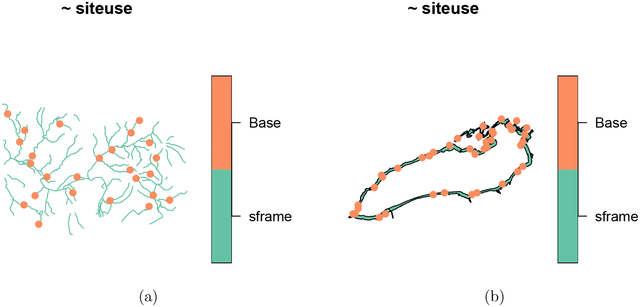
Equal probability GRTS sample of size 20 from the Illinois River data (a) and the Lake Ontario data (b).

R> plot(eqprob_linear, sframe = Illinois_River, pch = 19)

Notice how the sample units area spread throughout the reach segments. The same approach can be used to select GRTS sample of size 40 from Lake_Ontario, an areal resource of shoreline segments surrounding Lake Ontario, by running

R> set.seed(5)
R> eqprob_areal <- grts(Lake_Ontario, n_base = 40)

We visualize the sample overlain onto the sampling frame (Figure 4b) by running

R> plot(eqprob_areal, sframe = Lake_Ontario, pch = 19)

Notice how the sample units are spread throughout the shoreline.

To learn more about how the GRTS algorithm accommodates each of the three resource types (point, linear, areal), run ?grts and view the package vignettes (vignette(package = “spsurvey”). To learn more about the Illinois_River and Lake_Ontario data in spsurvey, run ?Illinois_River and ?Lake_Ontario, respectively.

3. Analysis

After collecting data at the design sites, population parameters can be estimated. Often times, these parameters are population proportions, means, or totals. Suppose τ represents a population total. Horvitz and Thompson (1952) showed that an unbiased estimator of τ is given by

$$\widehat{\tau }=\sum _{i=1}^n\frac{y_i}{{\pi }_i},$$ (1)

where n is the sample size, y_i is the response variable measured at s_i (the ith design site), and π_i is the inclusion probability of s_i. The term ${\pi }_i^{-1}$ is the reciprocal of π_i and is called a design weight. The design weight quantifies how many sites s_i represents in the sampling frame. Though Equation 1 was originally derived for finite populations, Cordy (1993) showed it remains unbiased for infinite populations. Other parameters like proportions and means are estimated using similar forms of Equation 1.

Horvitz and Thompson (1952) showed that an unbiased estimator of the variance of τˆ is given by

$$\widehat{\text{VAR}}(\widehat{\tau })=\sum _{i=1}^n\frac{\left(1-{\pi }_i\right)}{{\pi }_i^2}{y}_i^2+\sum _{i=1}^n\sum _{i\ne j}\frac{\left({\pi }_{ij}-{\pi }_i{\pi }_j\right)}{{\pi }_{ij}{\pi }_i{\pi }_j}{y}_i{y}_j,$$ (2)

where π_ij is the probability both s_i and s_j are included in the sample. In a finite population simple random sample, Equation 2 reduces to the following well-known formula:

$$\widehat{\text{VAR}}(\widehat{\tau })=\frac{N(N-n)}{n(n-1)}\sum _{i=1}^n{\left(y_i-\frac{\widehat{\tau }}{N}\right)}^2,$$ (3)

where N equals the number of sites in the sampling frame. Sen (1953) and Yates and Grundy (1953) derived a similar unbiased estimator of the variance of $\widehat{\tau }$. Both this estimator and Equation 2 rely on knowing the π_ij for all s_i and s_j. Calculating π_ij can be very challenging for more complicated designs, so Hartley and Rao (1962), Overton (1987), and Brewer (2002) proposed different approaches to approximating π_ij when estimating variances (as in Equation 2).

The aforementioned variance estimators and π_ij approximations do not incorporate the spatial locations of the s_i. Stevens and Olsen (2003) derived an estimator of the variance of τ that does incorporate the spatial locations of the s_i by conditioning on random properties of the GRTS sample. This variance estimator is called the local neighborhood variance estimator. The local neighborhood variance estimator of $\widehat{\tau }$ is denoted $\widehat{\text{VAR}}{(\widehat{\tau })}_{\text{lnb}}$ and is given by

$$\widehat{\text{VAR}}{(\widehat{\tau })}_{\text{lnb}}=\sum _{i=1}^n\sum _{s_j\in D\left(s_i\right)}{w}_{ij}{\left(\frac{y_j}{{\pi }_j}-\sum _{s_k\in D\left(s_i\right)}{w}_{ik}\frac{y_k}{{\pi }_k}\right)}^2,$$ (4)

where the w_ij are weights and D(s_i) is the set of design sites in s_i’s local neighborhood. Stevens and Olsen (2003) provide technical details and discuss how to determine the local neighborhoods. Equation 4 is useful for two reasons. First, it does not rely on π_ij. Second, incorporating the spatial locations of the s_i tends to reduce the variance of $\widehat{\tau }$ compared to a variance estimator that ignores spatial locations, which leads to narrower confidence intervals and more powerful hypothesis testing.

spsurvey provides a suite of functions for analyzing data. These functions implement the Horvitz-Thompson estimator (Equation 1) to estimate population parameters like proportions, means, and totals. The default variance estimator is the local neighborhood variance estimator (Equation 4), though the SRS, Horvitz-Thompson, and Yates-Grundy variance estimators as well as the π_ij approximations are also available. Next we show how to implement some of these analysis functions using the the NLA_PNW data in spsurvey. The NLA_PNW data is an ‘sf’ object with several variables measured at 96 lakes (treated as a whole) in the Pacific Northwest Region of the United States. There are five variables in NLA_PNW we will use throughout the rest of this section: WEIGHT, which represents a continuous design weight equaling the reciprocal of the site’s inclusion probability $\left({\pi }_i^{-1}\right)$; URBAN, which represents a categorical identifier based on whether the site is in an urban or non-urban area; STATE, which represents a categorical state identifier (California, Oregon, Washington); BMMI, which represents a continuous benthic macroinvertebrate multi-metric index; and NITR_COND, which represents a categorical nitrogen condition (Good, Fair, Poor). To load NLA_PNW into your global environment, run

R> data(“NLA_PNW”, package = “spsurvey”)

3.1. Categorical variable analysis

To analyze categorical variables in spsurvey, use the cat_analysis() function. cat_analysis requires a few arguments: dframe, a data frame or ‘sf’ object that contains the data; vars, the variables to analyze, and weight, the design weights. The cat_analysis function provides several pieces of output for each level of each variable in vars, including sample sizes, proportion estimates, total estimates, standard error estimates, margins of error (standard errors multiplied by a critical value), and confidence intervals. The proportion estimates are suffixed with a .P while the total estimates are suffixed with a .U (short-hand for unit total). Recall that the default local neighborhood variance estimator requires spatial coordinates. If dframe is a data frame, these are provided via the xcoord and ycoord arguments. If dframe is an ‘sf’ object, these are automatically taken from the ‘sf’ object’s geometry column. Additional variance estimation options are available via the vartype and jointprob arguments.

To perform categorical variable analysis of nitrogen condition, run

R> nitr <- cat_analysis(NLA_PNW, vars = “NITR_COND”, weight = “WEIGHT”)

To view the sample sizes, estimates, and 95% confidence intervals for the proportion of lakes in each nitrogen category, run

R> subset(nitr, + select = c(Category, nResp, Estimate.P, LCB95Pct.P, UCB95Pct.P))

	Category	nResp	Estimate.P	LCB95Pct.P	UCB95Pct.P
1	Fair	24	23.69392	11.55386	35.83399
2	Good	38	51.35111	36.78824	65.91398
3	Poor	34	24.95496	13.35359	36.55634
4	Total	96	100.00000	100.00000	100.00000

The confidence level can be changed using the conf argument. To view the sample sizes, estimates, and 95% confidence intervals for the total number of lakes in each nitrogen category, run

R> subset(nitr,
+    select = c(Category, nResp, Estimate.U, LCB95Pct.U, UCB95Pct.U))

	Category	nResp	Estimate.U	LCB95Pct.U	UCB95Pct.U
1	Fair	24	2530.428	1171.077	3889.780
2	Good	38	5484.120	3086.357	7881.883
3	Poor	34	2665.103	1375.258	3954.949
4	Total	96	10679.652	7903.812	13455.491

When vars is a vector, all variables are analyzed separately using a single call to cat_analysis(). Sometimes the goal is to estimate parameters for different subsets of the population – these subsets are called subpopulations. For example, to analyze nitrogen condition while treating each state as a separate subpopulation, run

R> nitr_subpop <- cat_analysis(NLA_PNW, vars = “NITR_COND”,
+    subpops = “STATE”, weight = “WEIGHT”)

To view the sample sizes and 95% confidence intervals for the total number of Oregon lakes in each nitrogen category, run

R> subset(nitr_subpop,
+    subset = Subpopulation == “Oregon”,
+    select = c(Subpopulation, Category, nResp, Estimate.U, LCB95Pct.U,
+      UCB95Pct.U))

	Subpopulation	Category	nResp	Estimate.U	LCB95Pct.U	UCB95Pct.U
5	Oregon	Fair	8	1298.8470	266.5980	2331.096
6	Oregon	Good	26	2854.3752	1533.3077	4175.443
7	Oregon	Poor	13	630.3551	241.3029	1019.407
8	Oregon	Total	47	4783.5773	3398.7997	6168.355

When subpops is a vector, all subpopulations are analyzed separately using a single call to cat_analysis(). When vars and subpops are both vectors, all combinations of variables and subpopulations are analyzed separately using a single call to cat_analysis().

Suppose the sampling design was stratified by the URBAN variable. To incorporate stratification by urban category, run

R> nitr_strat <- cat_analysis(NLA_PNW, vars = “NITR_COND”,
+    stratumID = “URBAN”, weight = “WEIGHT”)

To incorporate subpopulations (by state) and stratification (by urban category), run

R> nitr_strat_subpop <- cat_analysis(NLA_PNW, vars = “NITR_COND”,
+    subpops = “STATE”, stratumID = “URBAN”, weight = “WEIGHT”)

3.2. Continuous variable analysis

To analyze continuous variables in spsurvey, use the cont_analysis() function. Like cat_analysis(), cont_analysis() requires specifying the dframe, vars, and weight arguments. The cont_analysis() function provides several pieces of output for each variable in vars, including sample sizes, cumulative distribution function (CDF) estimates, percentile estimates, mean estimates, total estimates, standard error estimates, margins of error, and confidence intervals. The CDF, percentile, mean, and total estimates are returned in separate list elements and may be included or omitted using the statistics argument (by default, all quantities are estimated). As with cat_analysis(), the local neighborhood variance estimator is the default variance estimator.

To perform continuous variable analysis of benthic macroinvertebrate multi-metric index (BMMI), run

R> bmmi <- cont_analysis(NLA_PNW, vars = “BMMI”, weight = “WEIGHT”,
+    siteID = “SITE_ID”)

To view sample sizes, estimates, and 95% confidence intervals for the mean, run

R> subset(bmmi$Mean,
+    select = c(Indicator, nResp, Estimate, LCB95Pct, UCB95Pct))

	Indicator	nResp	Estimate	LCB95Pct	UCB95Pct
1	BMMI	96	56.50929	53.01609	60.00249

To visualize the CDF estimates and alongside their 95% confidence intervals, run

R> plot(bmmi$CDF)

The percentile output is contained in bmmi$Pct. By default, a few specific percentiles are estimated, though this can be changed via the pctval argument.

To analyze BMMI separately for each state, run

R> bmmi_state <- cont_analysis(NLA_PNW, vars = “BMMI”, subpops = “STATE”,
+    weight = “WEIGHT”)

To view the sample sizes, estimates, and 95% confidence intervals for the mean in each state, run

R> subset(bmmi_state$Mean,
+    select = c(Subpopulation, Indicator, nResp, Estimate, LCB95Pct,
+      UCB95Pct))

	Subpopulation	Indicator	nResp	Estimate	LCB95Pct	UCB95Pct
1	California	BMMI	19	50.48964	42.55357	58.42572
2	Oregon	BMMI	47	61.29675	56.23802	66.35548
3	Washington	BMMI	30	54.23036	48.06838	60.39234

To incorporate stratification (by urban category), run

R> bmmi_strat <- cont_analysis(NLA_PNW, vars = “BMMI”, stratumID = “URBAN”,
+    weight = “WEIGHT”)

To incorporate subpopulations (by state) and stratification (by urban category), run

R> bmmi_strat_state <- cont_analysis(NLA_PNW, vars = “BMMI”,
+    subpops = “STATE”, stratumID = “URBAN”, weight = “WEIGHT”)

3.3. Additional analysis approaches

Several other analysis options are available in spsurvey: relative risk analysis using relrisk_analysis(); attributable risk analysis using attrisk_analysis(); difference in risk analysis using diffrisk_analysis(); change analysis using change_analysis(); and trend analysis using trend_analysis(). The arguments for these functions are nearly identical to the arguments for cat_analysis() and cont_analysis(), with a few occasional exceptions.

The relative risk of an event (with respect to a stressor) is the ratio of two quantities. The numerator of the ratio is the probability the event occurs given exposure to the stressor. The denominator of the ratio is the probability the event occurs given no exposure to the stressor. Mathematically, the relative risk is defined as

$$RR=\frac{P(\text{ Event }\mid \text{ Stressor })}{P(\text{ Event }\mid \text{ No Stressor })},$$

where P(Event | Stressor) is the probability the event occurs given exposure to the stressor and P(Event | No Stressor) is the probability the event occurs given no exposure to the stressor. The attributable risk of an event (with respect to a stressor) is one minus a ratio of two quantities. The numerator of the ratio is the probability the event occurs given no exposure to the stressor. The denominator of the ratio is the overall probability the event occurs. Mathematically, the attributable risk is defined as

$$\text{AR}=1-\frac{\text{P}(\text{ Event }\mid \text{ No Stressor })}{\text{P}(\text{ Event })},$$

where P(Event) is the overall probability the event occurs.

Though relative risk and attributable risk are most often discussed in the medical literature, Van Sickle and Paulsen (2008) emphasize the usefulness of relative and attributable risk in the context of aquatic resources and stressors. The final risk metric available in spsurvey is difference in risk (with respect to a stressor). The difference in risk is the difference between the probability the event occurs given exposure to the stressor and the probability the event occurs given no exposure to the stressor. Mathematically, the difference in risk is defined as

$$RD=P(\text{ Event }\mid \text{ Stressor })-P(\text{ Event }\mid \text{ No Stressor }).$$

Because it is not a relative metric, the difference in risk complements the relative and attributable risks. The three risk metrics quantify several different aspects of risk and together to help provide a complete characterization of a resource’s risk (with respect to a stressor).

The risk analysis functions in spsurvey require four new arguments: vars_response, which indicates the response variables; vars_stressor, which indicates the stressor variables; response_levels, which indicates the two levels of the response variables (event and no event); and stressor_levels, which indicates the two levels of the stressor variables (stressor present and stressor not present). If the vars_response and vars_stressor arguments are vectors, all combinations of vars_response and vars_stressor are analyzed. Subpopulations and stratification are accommodated via the subpops and stratumID arguments, respectively.

Change and trend estimation are most commonly used to study the behavior of a resource through time. Change estimation focuses on comparing the resource at two time points. Parameters are estimated at each time point and the difference between the estimates is of interest. The variance of this difference incorporates the variability at each time point and the correlation between sites that are sampled at both time points. In trend estimation, parameters are estimated at each time point and a regression model fits a linear trend in the estimates through time. There are three available regression models: a simple linear regression model, a weighted linear regression model, and the mixed effects linear regression model from Piepho and Ogutu (2002).

The change and trend analysis functions in spsurvey require three new arguments: vars_cat, which indicates the categorical variables to estimate; vars_cont, which indicates the continuous variables to estimate; and a surveyID variable that distinguishes between the time points. The trend_analysis() function also requires the model_cat and model_cont arguments, which indicate the trend models for the categorical and continuous variables, respectively. As with the risk analysis functions, subpopulations and stratification are accommodated via the subpops and stratumID arguments, respectively.

4. Application

In this section, we use spsurvey to compare two sampling and analysis approaches: spatial and non-spatial. The spatial approach uses the GRTS algorithm for sampling and the local neighborhood variance estimator (Equation 4) for analysis. The non-spatial approach uses simple random sampling (SRS) and its variance estimator (Equation 3) for analysis. The data studied are from the United States Environmental Protection Agency’s 2012 National Lakes Assessment, a survey designed to monitor the status of lakes in the conterminous United States in 2012 (U.S. Environmental Protection Agency 2017).

We considered two variables in the NLA12 data: Atrazine presence (AP), a binary metric indicating whether Atrazine is present; and a continuous benthic macroinvertebrate multi-metric index (BMMI). Data were recorded at 1028 lakes for AP and 914 lakes for BMMI. By running

R> NLA12 <- sp_frame(NLA12)
R> summary(NLA12, formula = ~ AP + BMMI)

total	AP	BMMI
total:1030	N :694	Min. : 0.00
	Y :334	1st Qu.:33.00
	NA’s: 2	Median :43.90
		Mean :43.22
		3rd Qu.:54.60
		Max. :86.10
		NA’s :116

we see that the true proportion of lakes containing Atrazine is 0.3249, and the true mean BMMI of lakes is 43.22. By running

R> plot(NLA12, formula = ~ AP + BMMI)

we see that Atrazine presence is concentrated in the Upper Midwest (Figure 6a), while there is no clear spatial pattern for BMMI (Figure 6b). The data for each resource are treated as separate populations for the purposes of this section.

Figure 6:

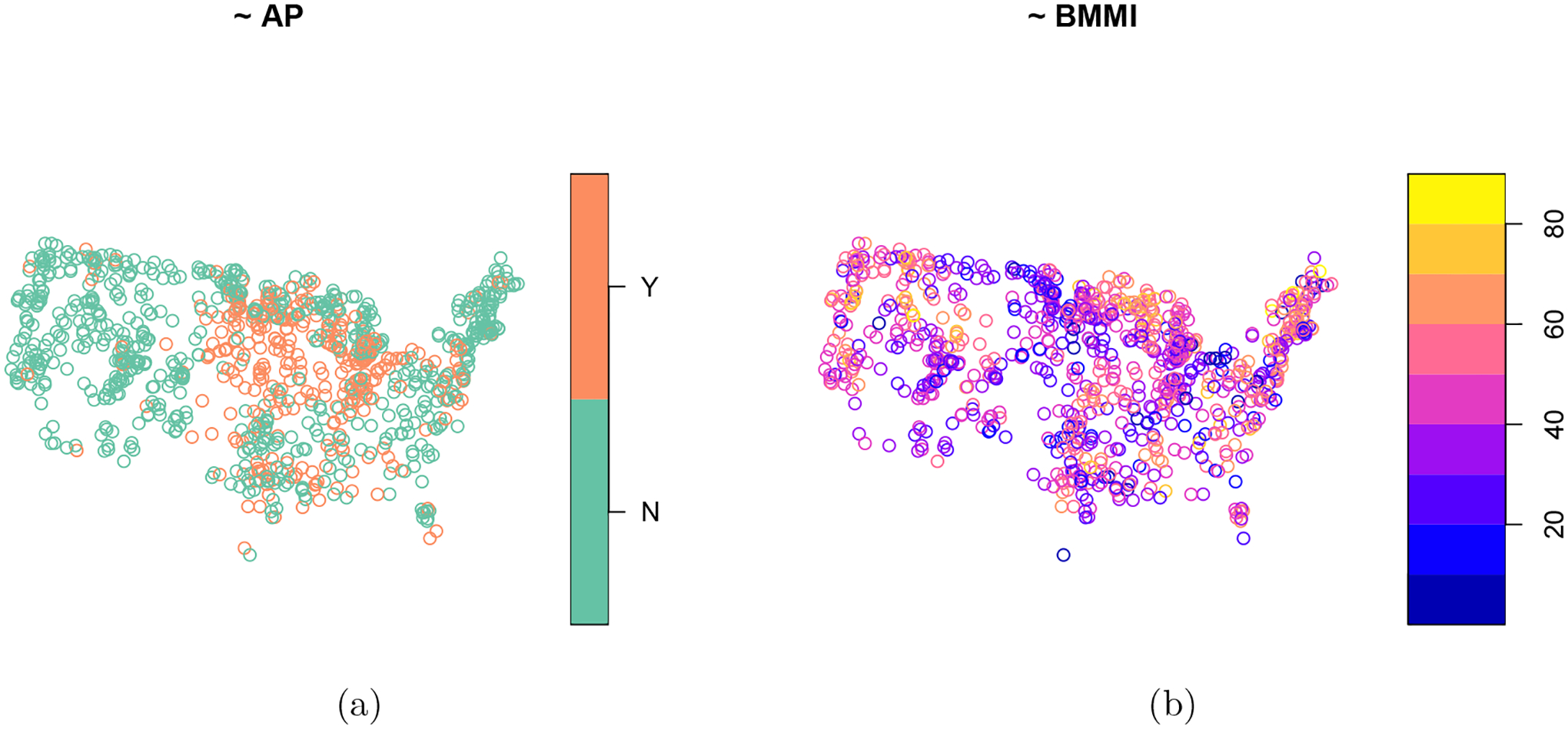
Spatial distributions of Atrazine presence (a) and a benthic macroinvertebrate multi-metric index (b) from the 2012 National Lakes Assessment.

A simulation study was used to compare the spatial and non-spatial approaches. First unstratified, equal probability samples of size 250 were selected from the Atrazine presence population (Figure 6a) using the GRTS and SRS algorithms. Then several quantities were computed: the sample’s spatial balance measured using Pielou’s evenness index; an estimate, denoted by $\widehat{p}$, of the true proportion of Atrazine presence, denoted by p; an estimate of the standard error of $\widehat{p}$; and an indicator variable measuring whether a 95% confidence interval for p contains 0.3249. This process was repeated 2000 times, and then the following summary metrics were computed: mean spatial balance; mean bias, measured as the average deviation of $\widehat{p}$ from p; root-mean-squared error, measured as the square root of the average squared deviation of $\widehat{p}$ from p; the 95% confidence interval coverage rate; and mean margin of error, measured as the average half-width of the 95% confidence interval for p. The same process was used to study BMMI. The spsurvey functions grts(), irs(), sp_balance(), cat_anlaysis(), and cont_analysis() were used during these simulations.

The Atrazine presence summary metrics are presented in Table 1. The mean spatial balance for the GRTS samples is lower than for the SRS samples. The Atrazine presence estimates from the GRTS and SRS samples both appear to be unbiased (mean bias near zero), but the root-mean-squared error of the SRS estimates is roughly 25% higher than root-meansquared error of the GRTS estimates. The spatial approach and the non-spatial approach both have confidence interval coverage near 95%. The mean margin of error for the non-spatial approach, however, is roughly 24% higher than for the spatial approach. Boxplots representing each simulation trial’s spatial balance and margin of error are displayed for both approaches in Figure 7.

Table 1:

Sampling algorithm (Algorithm), mean spatial balance (SPB), mean bias (Bias), root-mean-squared error (RMSE), 95% confidence interval coverage (Coverage), and mean margin of error (MOE) for 2000 simulation trials comparing the spatial and non-spatial approaches for studying Atrazine presence.

Algorithm	SPB	Bias	RMSE	Coverage	MOE
GRTS	0.0214	−0.0003	0.0206	0.9525	0.0406
SRS	0.0339	−0.0008	0.0258	0.9455	0.0505

Figure 7:

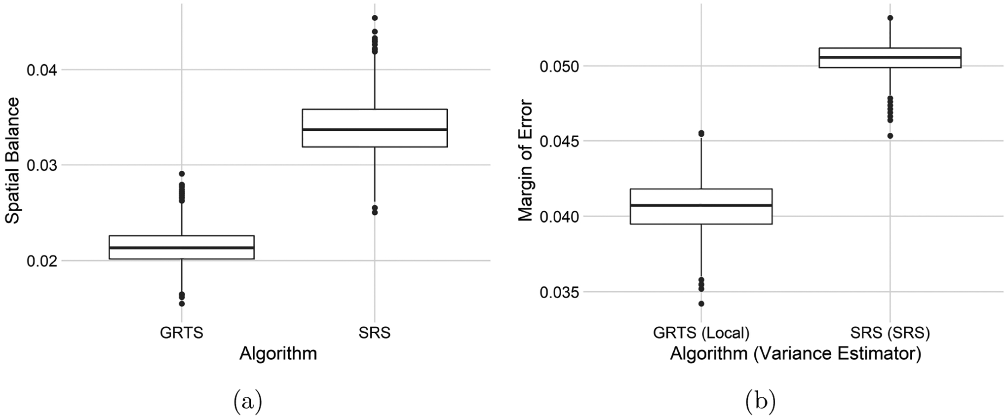
Boxplots of spatial balance (a) and margins of error (b) in the 2000 simulation trials comparing the spatial and non-spatial approaches for studying Atrazine presence.

The BMMI summary metrics are presented in Table 2. These results are similar to the Atrazine presence results: GRTS samples tend be more spatially balanced than SRS samples; the mean bias of estimates from the GRTS and SRS samples is near zero; root-mean-squared error from the SRS samples is roughly 10% higher than root-mean-squared error from the GRTS samples; confidence interval coverage is near 95% for both approaches; and the mean margin of error for the non-spatial approach is roughly 9% higher than the mean margin of error for the spatial approach. Boxplots representing each simulation trial’s spatial balance and margin of error are displayed for both approaches in Figure 8.

Table 2:

Samplilng algorithm (Algorithm), mean spatial balance (SPB), mean bias (Bias), root-mean-squared error (RMSE), 95% confidence interval coverage (Coverage), and mean margin of error (MOE) for 2000 simulation trials comparing the spatial and non-spatial approaches for studying BMMI.

Algorithm	SPB	Bias	RMSE	Coverage	MOE
GRTS	0.0213	0.0063	0.7655	0.9520	1.5303
SRS	0.0336	0.0134	0.8421	0.9440	1.6668

Figure 8:

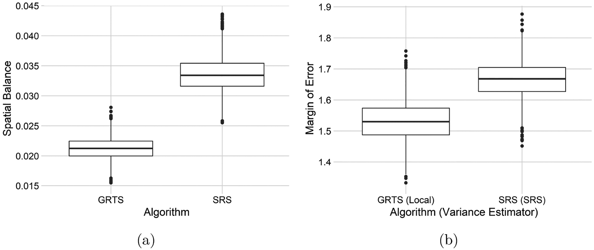
Boxplots of spatial balance (a) and margins of error (b) for 2000 simulation trials comparing the spatial and non-spatial approaches for studying BMMI.

The advantages of the spatial approach in this simulation study are clear. The GRTS samples are more spatially balanced than the SRS samples. The estimates from the GRTS samples are unbiased and have lower root-mean-squared error than estimates from the SRS samples. The spatial approach has smaller margins of error than the non-spatial approach (while re-taining proper coverage). This implies that confidence intervals from the spatial approach are narrower (more precise) than confidence intervals from the non-spatial approach.

For Atrazine presence, the non-spatial approach has a roughly 25% higher root-mean-squared error than the spatial approach. For BMMI, the non-spatial approach have a roughly 10% higher root-mean-squared error than the spatial approach. The relative root-mean-squared error increase is larger for Atrazine presence than BMMI. This is likely because Atrazine presence has a stronger spatial pattern (Figure 6a) than BMMI (Figure 6b), suggesting that the stronger the spatial pattern, the greater the advantage of the spatial approach compared to the non-spatial approach.

5. Discussion

spsurvey offers a suite of tools for design-based statistical inference, with a focus on spatial data. The summary() and plot() functions summarize and visualize data. The grts() function selects spatially balanced samples from point, linear, and areal resources and flexibly accommodates stratification, varying inclusion probabilities, legacy (historical) sites, minimum distance between sites, and two options for replacement sites (reverse hierarchical ordering and nearest neighbor). The sp_balance() function computes the spatial balance of a sample. The sp_rbind() binds together the design sites into a single ‘sf’ object. spsurvey’s analysis functions are used for categorical variable analysis (cat_analysis()), continuous variable analysis cont_analysis()), relative risk analysis (relrisk_analysis), attributable risk analysis (attrisk_analysis()), difference in risk analysis (diffrisk_analysis), change analysis (change_analysis), and trend analysis (trend_analysis). Aside from these core functions, spsurvey has several other specialized functions to perform cluster sampling and analysis, cumulative distribution function (CDF) hypothesis testing, panel designs, power analysis, design weight adjustments, and more.

We plan to continually update spsurvey so that it is reflective of new research. Because spsurvey depends on sf for sampling and survey (Lumley 2020) for analysis, spsurvey may also change alongside these packages. spsurvey is an open-source project, and we want it to be as helpful and user-friendly as possible. To help us accomplish these goals, we encourage users to give us feedback regarding desired features, bug fixes, and other suggestions for spsurvey.

Figure 5:

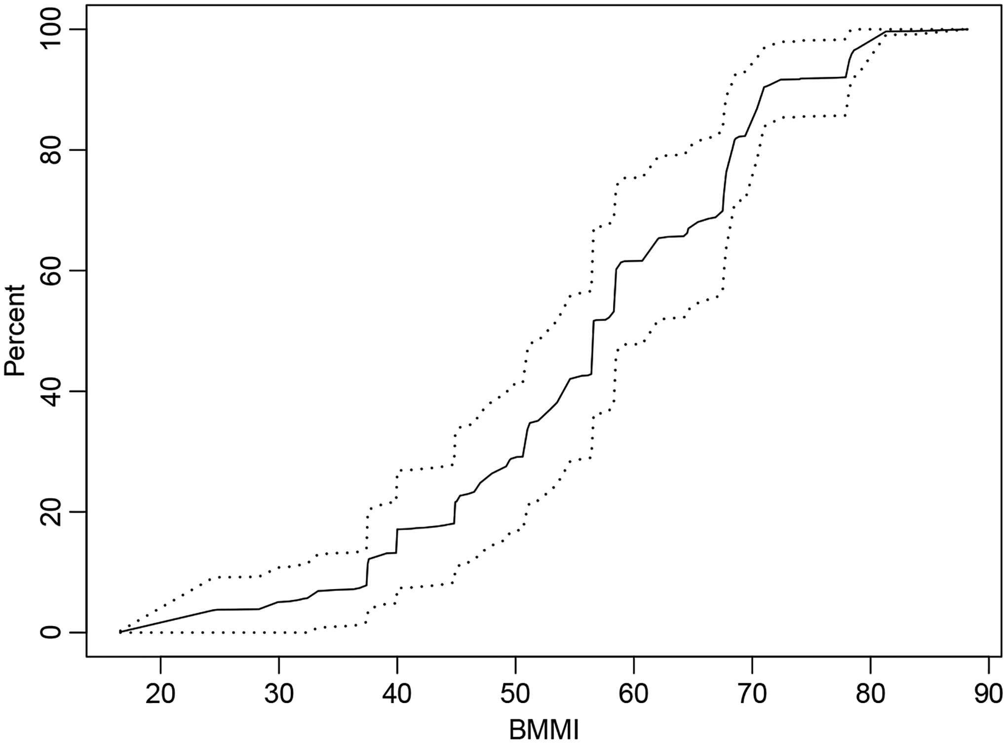
BMMI cumulative distribution function (CDF) estimates (solid line) and 95% confidence intervals (dashed lines).

Data and code availability

All writing, code, and data associated with this manuscript are available for viewing and download in a supplementary R package located at the GitHub repository: https://github.com/USEPA/spsurvey.manuscript. Instructions for use are included in the repository’s README. This supplementary R package contains a replication script that can be used to reproduce all results presented in the manuscript. Replicating the simulation study could take 10–60 minutes, but results are provided as .rda files in the supplementary R package. Moreover, all necessary replication codes can be found on the journal’s website.

References

- Barabesi L, Franceschi S (2011). “Sampling Properties of Spatial Total Estimators under Tessellation Stratified Designs.” Environmetrics, 22(3), 271–278. doi: 10.1002/env.1046. [DOI] [Google Scholar]
- Benedetti R, Piersimoni F (2017). “A Spatially Balanced Design with Probability Function Proportional to the Within Sample Distance.” Biometrical Journal, 59(5), 1067–1084. doi: 10.1002/bimj.201600194. [DOI] [PubMed] [Google Scholar]
- Benedetti R, Piersimoni F, Postiglione P (2017). “Spatially Balanced Sampling: A Review and A Reappraisal.” International Statistical Review, 85(3), 439–454. doi: 10.1111/insr.12216. [DOI] [Google Scholar]
- Brewer K (2002). Combined Survey Sampling Inference: Weighing Basu’s Elephants. Arnold. URL https://books.google.at/books?id=JKw6f61bnMEC.
- Cordy CB (1993). “An Extension of the Horvitz-Thompson Theorem to Point Sampling from a Continuous Universe.” Statistics & Probability Letters, 18(5), 353–362. doi: 10.1016/0167-7152(93)90028-H. [DOI] [Google Scholar]
- Dumelle M, Kincaid TM, Olsen AR, Weber MH (2023). spsurvey: Spatial Sampling Design and Analysis. R package version 5.4.1, URL https://CRAN.R-project.org/package=spsurvey. [DOI] [PMC free article] [PubMed]
- Foster SD (2021). “MBHdesign: An R Package for Efficient Spatial Survey Designs.” Methods in Ecology and Evolution, 12(3), 415–420. doi: 10.1111/2041-210x.13535. [DOI] [Google Scholar]
- Foster SD, Hosack GR, Lawrence E, Przeslawski R, Hedge P, Caley MJ, Barrett NS, Williams A, Li J, Lynch T, Dambacher JM, Sweatman HPA, Hayes KR (2017). “Spatially Balanced Designs that Incorporate Legacy Sites.” Methods in Ecology and Evolution, 8(11), 1433–1442. doi: 10.1111/2041-210X.12782. [DOI] [Google Scholar]
- Foster SD, Hosack GR, Monk J, Lawrence E, Barrett NS, Williams A, Przeslawski R (2020). “Spatially Balanced Designs for Transect-Based Surveys.” Methods in Ecology and Evolution, 11(1), 95–105. doi: 10.1111/2041-210X.13321. [DOI] [Google Scholar]
- Grafström A (2012). “Spatially Correlated Poisson Sampling.” Journal of Statistical Planning and Inference, 142(1), 139–147. doi: 10.1016/j.jspi.2011.07.003. [DOI] [Google Scholar]
- Grafström A, Lisic J (2019). BalancedSampling: Balanced and Spatially Balanced Sampling. R package version 1.5.5, URL https://CRAN.R-project.org/package=BalancedSampling.
- Grafström A, Lundström NL, Schelin L (2012). “Spatially Balanced Sampling through the Pivotal Method.” Biometrics, 68(2), 514–520. doi: 10.1111/j.1541-0420.2011.01699.x. [DOI] [PubMed] [Google Scholar]
- Grafström A, Lundström NLP (2013). “Why Well Spread Probability Samples Are Balanced.” Open Journal of Statistics, 3(1), 36–41. doi: 10.4236/ojs.2013.31005. [DOI] [Google Scholar]
- Grafström A, Matei A (2018). “Spatially Balanced Sampling of Continuous Populations.” Scandinavian Journal of Statistics, 45(3), 792–805. doi: 10.1111/sjos.12322. [DOI] [Google Scholar]
- Hartley HO, Rao JNK (1962). “Sampling with Unequal Probabilities and without Replacement.” The Annals of Mathematical Statistics, 33(2), 350–374. doi: 10.1214/aoms/1177704564. [DOI] [Google Scholar]
- Horvitz DG, Thompson DJ (1952). “A Generalization of Sampling without Replacement from a Finite Universe.” Journal of the American Statistical Association, 47(260), 663–685. doi: 10.2307/2280784. [DOI] [Google Scholar]
- Kruskal W, Mosteller F (1979a). “Representative Sampling, I: Non-Scientific Literature.” International Statistical Review, pp. 13–24. doi: 10.2307/1403202. [DOI] [Google Scholar]
- Kruskal W, Mosteller F (1979b). “Representative Sampling, II: Scientific Literature, Excluding Statistics.” International Statistical Review, pp. 111–127. doi: 10.2307/1402564. [DOI] [Google Scholar]
- Kruskal W, Mosteller F (1979c). “Representative Sampling, III: The Current Statistical Literature.” International Statistical Review, pp. 245–265. doi: 10.2307/1402647. [DOI] [Google Scholar]
- Lohr SL (2009). Sampling: Design and Analysis. 2nd edition. Cengage Learning. [Google Scholar]
- Lumley T (2020). survey: Analysis of Complex Survey Samples. R package version 4.0, URL https://CRAN.R-project.org/package=survey.
- McDonald T, McDonald A (2020). SDraw: Spatially Balanced Samples of Spatial Objects. R package version 2.1.13, URL https://CRAN.R-project.org/package=SDraw.
- Overton WS (1987). “A Sampling and Analysis Plan for Streams in the National Surface Water Survey.” Manuscript, Department of Statistics, Oregon State University, Corvallis, Oregon. [Google Scholar]
- Pantalone F, Benedetti R, Piersimoni F (2022). “Spbsampling: An R Package for Spatially Balanced Sampling.” Journal of Statistical Software, 103, 1–22. doi: 10.18637/jss.v103.c02. [DOI] [Google Scholar]
- Pebesma E (2018). “Simple Features for R: Standardized Support for Spatial Vector Data.” The R Journal, 10(1), 439–446. doi: 10.32614/RJ-2018-009. [DOI] [Google Scholar]
- Pielou EC (1966). “The Measurement of Diversity in Different Types of Biological Collections.” Journal of Theoretical Biology, 13, 131–144. doi: 10.1016/0022-5193(66)90013-0. [DOI] [Google Scholar]
- Piepho HP, Ogutu JO (2002). “A Simple Mixed Model for Trend Analysis in Wildlife Populations.” Journal of Agricultural, Biological, and Environmental Statistics, 7(3), 350–360. doi: 10.1198/108571102366. [DOI] [Google Scholar]
- Robertson B, McDonald T, Price C, Brown J (2018). “Halton Iterative Partitioning: Spatially Balanced Sampling via Partitioning.” Environmental and Ecological Statistics, 25(3), 305–323. doi: 10.1007/s10651-018-0406-6. [DOI] [Google Scholar]
- Robertson BL, Brown JA, McDonald T, Jaksons P (2013). “BAS: Balanced Acceptance Sampling of Natural Resources.” Biometrics, 69(3), 776–784. doi: 10.1111/biom.12059. [DOI] [PubMed] [Google Scholar]
- Särndal CE, Swensson B, Wretman J (2003). Model Assisted Survey Sampling. Springer-Verlag. [Google Scholar]
- Sen AR (1953). “On the Estimate of the Variance in Sampling with Varying Probabilities.” Journal of the Indian Society of Agricultural Statistics, 5(1194), 127. [Google Scholar]
- Shannon CE (1948). “A Mathematical Theory of Communication.” The Bell System Technical Journal, 27(3), 379–423. doi: 10.1002/j.1538-7305.1948.tb01338.x. [DOI] [Google Scholar]
- Stevens D, Olsen A (2003). “Variance Estimation for Spatially Balanced Samples of Environmental Resources.” Environmetrics, 14(6), 593–610. doi: 10.1002/env.606. [DOI] [Google Scholar]
- Stevens D, Olsen A (2004). “Spatially Balanced Sampling of Natural Resources.” Journal of the American Statistical Association, 99(465), 262–278. doi: 10.1198/016214504000000250. [DOI] [Google Scholar]
- Urquhart NS, Kincaid TM (1999). “Designs for Detecting Trend from Repeated Surveys of Ecological Resources.” Journal of Agricultural, Biological, and Environmental Statistics, pp. 404–414. doi: 10.2307/1400498. [DOI] [Google Scholar]
- US Environmental Protection Agency (2017). “National Lakes Assessment 2012.” Technical Report EPA841-R-16–114, The Office of Water and The Office of Research and Development, Washington, DC. URL https://www.epa.gov/national-aquatic-resource-surveys/national-lakes-assessment-2012-technical-report. [Google Scholar]
- Van Sickle J, Paulsen SG (2008). “Assessing the Attributable Risks, Relative Risks, and Regional Extents of Aquatic Stressors.” Journal of the North American Benthological Society, 27(4), 920–931. doi: 10.1899/07-152.1. [DOI] [Google Scholar]
- Walvoort D, Brus D, De Gruijter J (2022). Spatial Coverage Sampling and Random Sampling from Compact Geographical Strata. R package version 0.4–1, URL https://CRAN.R-project.org/package=spcosa.
- Walvoort DJJ, Brus DJ, De Gruijter JJ (2010). “An R Package for Spatial Coverage Sampling and Random Sampling from Compact Geographical Strata by k-means.” Computers & Geosciences, 36(10), 1261–1267. doi: 10.1016/j.cageo.2010.04.005. [DOI] [Google Scholar]
- Wang JF, Jiang CS, Hu MG, Cao ZD, Guo YS, Li LF, Liu TJ, Meng B (2013). “Design-Based Spatial Sampling: Theory and Implementation.” Environmental Modelling & Software, 40, 280–288. doi: 10.1016/j.envsoft.2012.09.015. [DOI] [Google Scholar]
- Yates F, Grundy PM (1953). “Selection without Replacement from within Strata with Probability Proportional to Size.” Journal of the Royal Statistical Society B, 15(2), 253–261.doi: 10.1111/j.2517-6161.1953.tb00140.x. [DOI] [Google Scholar]
Associated Data
This section collects any data citations, data availability statements, or supplementary materials included in this article.
Data Availability Statement