CascadeNet for hysterectomy prediction in pregnant women due to placenta accreta spectrum

Abstract

In severe cases, placenta accreta spectrum (PAS) requires emergency hysterectomy, endangering the life of both mother and fetus. Early prediction may reduce complications and aid in management decisions in these high-risk pregnancies. In this work, we developed a novel convolutional network architecture to combine MRI volumes, radiomic features, and custom feature maps to predict PAS severe enough to result in hysterectomy after fetal delivery in pregnant women. We trained, optimized, and evaluated the networks using data from 241 patients, in groups of 157, 24, and 60 for training, validation, and testing, respectively. We found the network using all three paths produced the best performance, with an AUC of 87.8, accuracy 83.3%, sensitivity of 85.0, and specificity of 82.5. This deep learning algorithm, deployed in clinical settings, may identify women at risk before birth, resulting in improved patient outcomes.

1. INTRODUCTION

The human placenta is a critical and complex organ that plays a key role in a successful pregnancy. It grows as the fetus grows during pregnancy, providing the required oxygen and nutrition to the growing fetus and the vital maternal-fetal exchanges. Complications can prove harmful to both the mother and child. One such complication is placenta accreta spectrum, or PAS, when the placenta remains attached during delivery^{1, 2}. In cases of PAS, severe bleeding can occur and necessitate the emergency removal of the uterus to preserve the life of the mother. These emergency procedures result in greater blood loss and an increased risk of complications^3–5. Thus, the early prediction of when a hysterectomy might be required is of interest to both patients and physicians. This is especially important as the incidence rate of PAS is increasing⁶.

The prediction of hysterectomy due to PAS has been explored using radiomics, with the best model performing with an area under the curve (AUC) of 0.80 for a cohort of 62 patients^{7, 8}. In this study, we aim to implement a novel deep learning architecture called CascadeNet for prediction of hysterectomy in women using data derived from clinical MRI. Along with the T2-weighted volumetric MRI data, we extract radiomic features from the MRI data and custom feature maps which can be treated as an additional path in the network. Therefore, three different CascadeNet architectures will be considered and compared.

2. METHODS

2.1. Data

Our dataset contains 241 T2-weighted MRI volumes (1.5T) from 241 pregnant women, separated into two classes based on clinical outcome: those who eventually had a hysterectomy (88), and those who did not (153). The in-plane size was 256 × 256 pixels for all but 3 patients, which were zero-padded to have an in-plane size of 256 × 256 pixels. The slice thickness for all patients was 7.0 mm, with the total number of slices ranging between 28 and 62. The in-plane resolution ranged from 1.055 × 1.055 mm² to 1.953 × 1.953 mm² across all patients. The 241 patients were split into three groups for the network: training (N=157), validation (N=24), and testing (N=60). Patient distributions are shown in Table I.

Table I.

Patient distribution per group.

	Training	Training (Augmented)	Validation	Testing
Hysterectomy	56	168	12	20
No Hysterectomy	101	202	12	40
Total	157	370	24	60

2.2. Preprocessing

The input 3D MRI volumes were resized to 192 × 192 × 25 voxels using linear interpolation to create a uniform data size for the network. Due to the imbalanced number of patients, the training dataset was augmented using an additional resizing technique as shown in Figure 1. The original MRI were either cropped or padded in the in-plane direction by 15% before being resized using linear interpolation to 192 × 192 × 25 voxels. All 56 hysterectomy patients in the training dataset were augmented using both methods to produce a total of 168 volumes. For the normal patients, the average in-plane resolution was found to be 1.3 × 1.3 mm². Patients with resolutions below this were augmented using the crop method while those with resolutions greater than 1.3 × 1.3 mm² were augmented using the padding method. Thus, the total number of normal patients in the training group was doubled to 202 patients, bringing the total training dataset to 370 patients, and improving the ratio of hysterectomy to normal patients from approximately 1:2 to 4:5.

Figure 1.

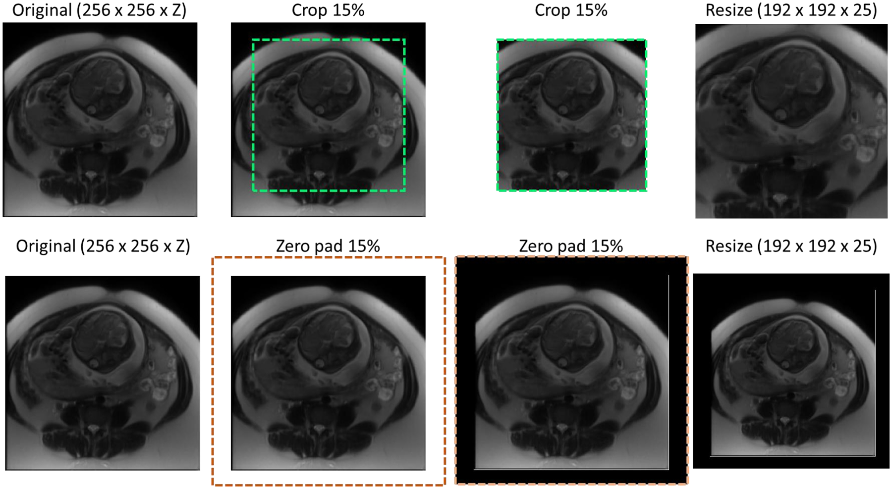
Cropping (top row) and padding (bottom row) augmentation procedures, where Z denotes the number of slices in the original MRI.

2.3. Radiomic Features

For extracting the radiomic features, manual segmentations of the uterus and placenta were first obtained from a radiologist and used as two individual masks. A total of 214 radiomic features were extracted using PyRadiomics, including shape, gray level co-occurrence, gray level run length, gray level size zone, gray level dependance, neighbor gray tone difference, and first order statistics⁹, with 107 features extracted from the placenta region and 107 from the uterus region.

2.4. Topographic Feature Maps

Novel topographic feature maps were created to provide additional insight into the texture of the placenta and surrounding regions. For inter-subject comparability of the topography maps, we normalized the placenta map by centered the centroid of the placenta. Figure 2 shows a sample topography map using the distance of the surface points from POV as the plotted feature. We used the same topography-based scanning and mapping scheme to extract and plot different features. For some features, a patch-based feature extraction is used to study the local properties of the placenta surface on MRI. In this study we extract the following features:

Figure 2.

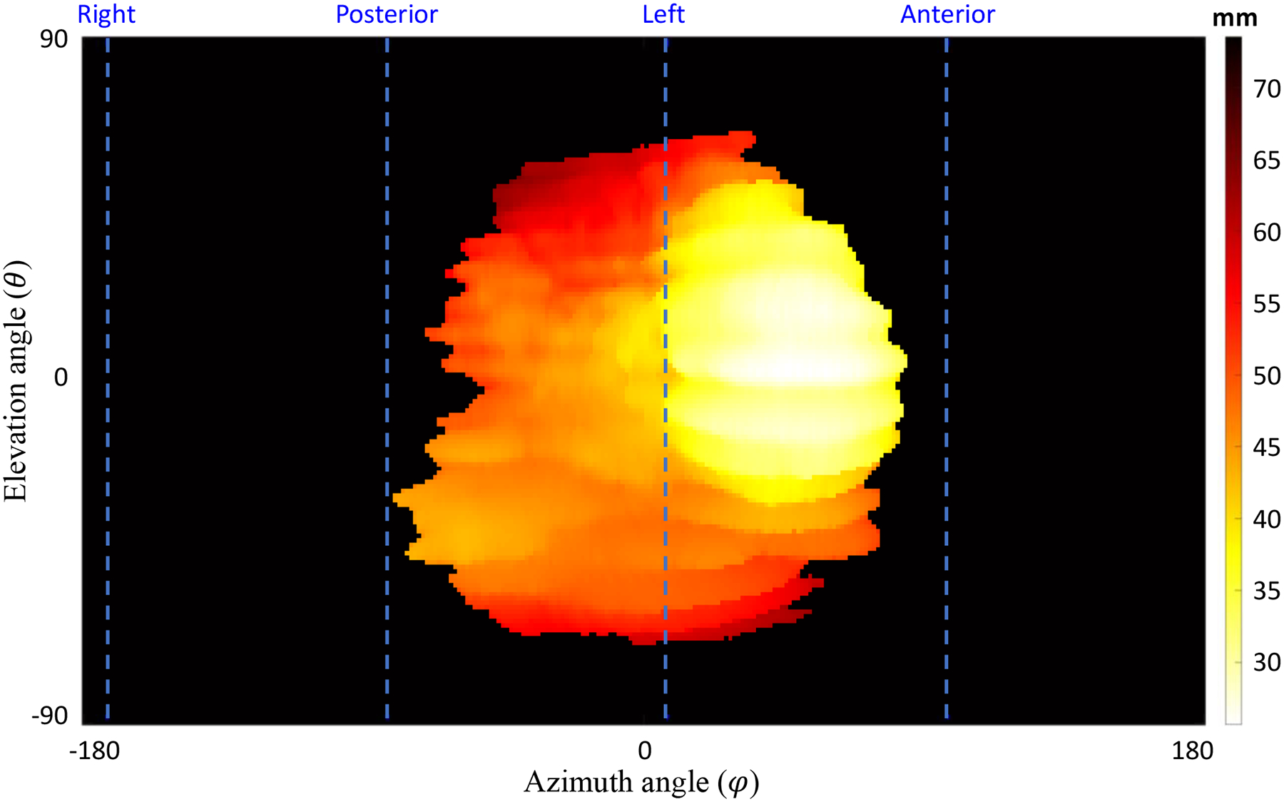
Topographic map. The distance of the maternal side surface points of the placenta from the POV for a sample case. The dashed lines show anterior, posterior, right, and left orientations (in this case the placenta is located at the left side and expanded toward posterior and anterior. The top and bottom parts of the topography map show the superior and inferior sides, respectively.

Distance: distance of placenta surface point from the POV is used as a feature that reflects some of topological characteristics of the placenta. We plotted two distance topography maps one for the fetal and one for the maternal side of the placenta.

Placenta thickness: the distance between the fetal side and maternal side surface points on each scanning ray is measured as the placenta thickness in that direction.

Surface intensity: The intensity of the image at the surface points. We generated two intensity maps one for the fetal side and one for the maternal side.

Local average of intensities: The average of patch intensities used as one feature to be plotted. This map is affected less by artifacts and noise observed on surface intensity maps. We plotted two average intensity maps, one for the fetal side and one for the maternal side.

Local standard deviation of the intensities: The standard deviation (STD) of intensities within each patch shows the roughness of intensity distribution around placenta border at each region. We plotted two maps for local standard deviation of the intensities, one for the fetal side and one for the maternal side.

For the patch-based feature extraction, we used a patch size of 11 × 11 × 11 voxels.

2.5. CascadeNet Architecture Options

We designed our innovative cascade deep learning architecture to extract deep learning-based features from medical images using a fully-connected architecture (Figure 3). The network is comprised of a main stem (Level 1A – 1D) and down-scaling stems (Levels 2–4). In the down-scaling stems, the input is sampled to create down-sampled images in order to extract deep learning features across different scales of the image. The goal of this process is to obtain more features related to both fine details and general structures. Figure 2 shows a block diagram of the cascade network with four scaling levels. During each down-scaling level, two convolutions are applied before the features are concatenated back into the main stem of the network. The main stem is comprised of four parts. For the first part, Level 1A, the input undergoes two convolutions, followed by max pooling with a 3 × 3 kernel and a stride of 2. The second part begins by concatenating the output of Level 1A with the output of Level 2 along the filter dimension, before performing a convolution and max pooling. Level 1C performs similarly to Level 1B. In Level 1D, the final sub-stem concatenation is performed, and the data enter the output stem. This part of the network consists of two sets of max pooling and convolution pairs, followed by an average pooling layer, a drop-out layer, and a flattening layer. Finally, two dense layers are used to create a prediction. All convolutions in the network utilize batch normalization and a sigmoid activation function. The kernel size for each convolution varies depending on the layer. As only 25 MRI slices are used, the kernel in that dimension is periodically left at 1. The kernel size for the in-plane dimensions are 3 × 3, except for the second convolution in the sub-stems, where the kernel is 2 × 2.

Figure 3.

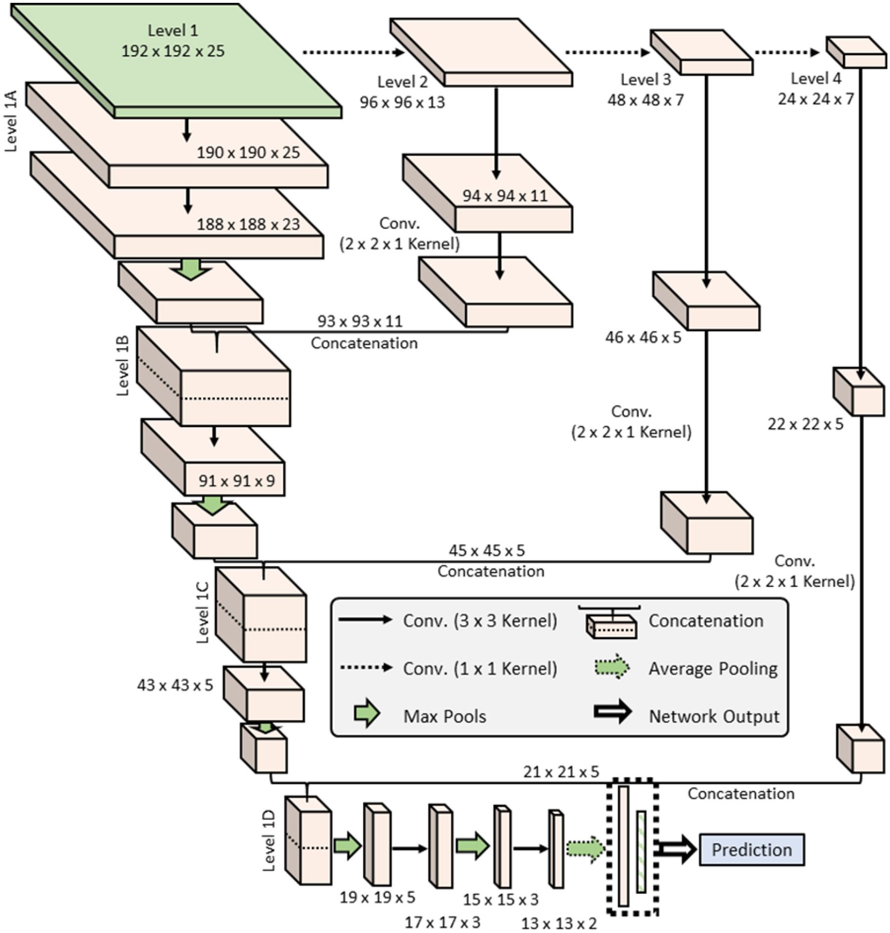
The basic architecture for the Cascade Network.

Deep learning and radiomics approaches have been demonstrated for the prediction and diagnosis of placental conditions. However, the combination of radiomic features and deep learning features into a combined system for placenta assessment has not been studied. In addition, the feature maps of the placenta mentioned previously could provide information unavailable in the clinical MRI. To combine these three data sources, we created a three-path version of the network (Figure 4). A 1D array of radiomic features are fed into two dense layers before being combined in a final dense layer for prediction (Figure 5). The final path is added for the feature maps using a 2D version of the original CascadeNet architecture, with a few minor changes. As the data is 2D, the convolutional layers were also switch to 2D. All convolutional kernel sizes are 3 × 3, except for the final convolution in the Level 2 sub-step, which is 2 × 2. Instead of extracting features from all channels of the feature map at once, features are extracted channel-by-channel and concatenated before being fed into a final dense layer for prediction (Figure 5). This ensures features from each channel are preserved until the final dense layer. The use of maternal serum screening data as an input to the deep learning algorithm is also possible as a fourth path, with an architecture similar to that of the radiomics data.

Figure 4.

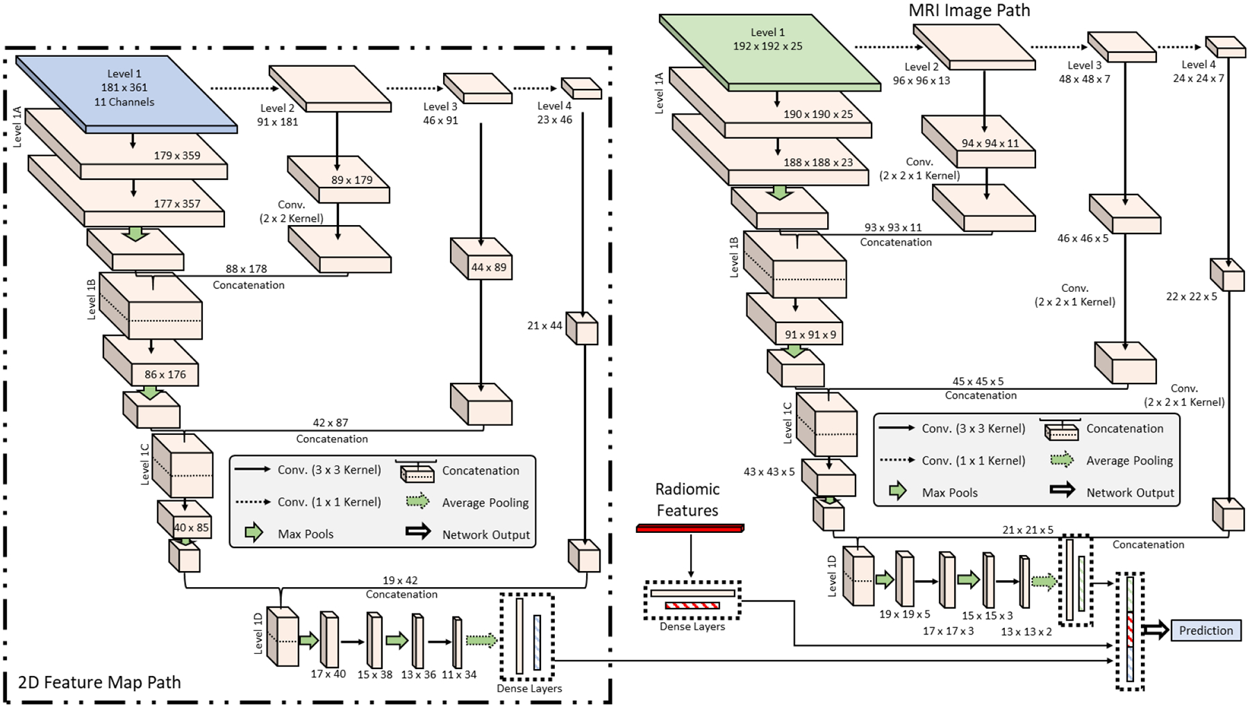
Three-path version of the network. The three paths are a 1D array of radiomic values, a 2D feature map with multiple channels, and a 3D MRI.

Figure 5.

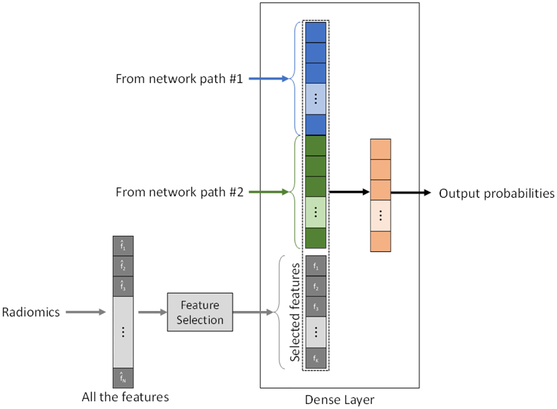
The integration between radiomic features and deep learning features at the dense layer.

As there are several proposed versions of the CascadeNet architecture, training can be performed in several ways depending on the inputs: (1) 3D MRI alone, (2) 3D MRI and 2D topographic feature maps, and (3) 3D MRI, 2D topographic feature maps, and 1D radiomics. The network is trained using the RMSProp optimizer in TensorFlow, with the learning rate set to exponential decay. Binary cross entropy was used as the loss function, with a weighting factor of 1:1.5 (normal:hysterectomy) to account for the imbalanced classes. During training, the dataset is shuffled after every epoch. Due to the nonsymmetric nature of the data, no augmentation was used. The networks were built on a CentOS 7 system with TensorFlow version 2.4 running in Docker. Training is conducted on an NVIDIA A6000 GPU. Each network was extensively optimized independently to produce a model with the best performance based on the validation data results. The evaluation metric used were patient-level accuracy, sensitivity, specificity, and AUC. Once the ideal model for each network was found, the model was evaluated on the reserved testing dataset.

3. RESULTS

Results from each independently optimized and tuned network when evaluated on the testing data (40 normal patients, 20 hysterectomy) are shown in Table II.

Table II.

Results from each CascadeNet architecture when evaluated on the testing data (N = 60).

Network Architecture	Accuracy (%)	Sensitivity (%)	Specificity (%)	AUC
3D MRI alone	80.0	85.0	77.5	85.4
3D MRI and 2D Topographic Map	81.7	85.0	80.0	87.0
3D MRI, 2D Topographic Map, and 1D Radiomics	83.3	85.0	82.5	87.8

As can be seen from the table, when only the 3D MRI data was used as an input, the network produced an accuracy of 80% (48 out of 60 correct predictions) and AUC of 85.4, along with sensitivity and specificity of 85.0% and 77.5% respectively. The addition of the 2D topographic feature map data produced an accuracy of 81.7% (49/60 correct) compared to 80.0% just using the 3D MRI data alone, but improved the AUC to 87.0, compared to 85.4 mentioned above. Finally, when all three inputs were utilized, the network produced an accuracy of 83.3% (50/60 correct), the highest of all three networks tested. The AUC was 87.8, a slight improvement over that of the two-path version.

4. DISCUSSION

All three Cascade networks displayed similar performance, which suggests the bulk of the predictive ability of the network was drawn from the volumetric MRI data. However, the addition of the feature maps improved the AUC of the network to 87.0. The addition of radiomic features to both the 3D MRI data and the 2D feature maps only slightly improved the AUC to 87.8, with an accuracy of the network to 83.3% (50/60 correct). The combination of sensitivity and specificity also improved, with both values being over 80%.

There were several limitations in this study. First, this work was conducted retrospectively, and thus could have unintended bias included in the design. Second, the patient groups for the study were imbalanced, with far fewer patients in the hysterectomy dataset. This could reduce the generalizability of the models. Finally, as each network was optimized manually, it is possible some additional improvements could be made with further tuning. Radiomics features and the 2D feature maps could also be considered in networks of their own to gauge their usability for PAS prediction.

5. CONCLUSION

In this work, we developed a novel CNN architecture for predicting patients which would undergo hysterectomy due to placenta accreta. The network was evaluated under three scenarios, with the network utilizing the 3D MRI data, 2D topographic feature maps, and the 1D radiomics vector found to perform the best on the testing data (accuracy of 83.3%). Future work will increase the number of patients used in the study and explore results when only the 2D feature maps are used for prediction.

REFERENCES

- [1].Strauss F, Benirschke K, and Driscoll SG, [Unusual Shapes of the Placenta. Placenta Accreta] Springer, (1967). [Google Scholar]
- [2].Maldjian C, Adam R, Pelosi M, Pelosi III M, Rudelli RD, and Maldjian J, “MRI appearance of placenta percreta and placenta accreta,” Magnetic resonance imaging, 17(7), 965–971 (1999). [DOI] [PubMed] [Google Scholar]
- [3].Briery CM, Rose CH, Hudson WT, Lutgendorf MA, Magann EF, Chauhan SP, and Morrison JC, “Planned vs emergent cesarean hysterectomy,” American journal of obstetrics and gynecology, 197(2), 154. e1–154. e5 (2007). [DOI] [PubMed] [Google Scholar]
- [4].Machado LS, “Emergency peripartum hysterectomy: incidence, indications, risk factors and outcome,” North American journal of medical sciences, 3(8), 358 (2011). [DOI] [PMC free article] [PubMed] [Google Scholar]
- [5].Kong X, Kong Y, Yan J, Hu J-J, Wang F-F, and Zhang L, “On opportunity for emergency cesarean hysterectomy and pregnancy outcomes of patients with placenta accreta,” Medicine, 96(39), (2017). [DOI] [PMC free article] [PubMed] [Google Scholar]
- [6].Jauniaux E, Kingdom JC, and Silver RM, “A comparison of recent guidelines in the diagnosis and management of placenta accreta spectrum disorders,” Best Practice & Research Clinical Obstetrics & Gynaecology, 72, 102–116 (2021). [DOI] [PubMed] [Google Scholar]
- [7].Do QN, Lewis MA, Madhuranthakam AJ, Xi Y, Bailey AA, Lenkinski RE, and Twickler DM, “Texture analysis of magnetic resonance images of the human placenta throughout gestation: a feasibility study,” PloS one, 14(1), e0211060 (2019). [DOI] [PMC free article] [PubMed] [Google Scholar]
- [8].Do QN, Lewis MA, Xi Y, Madhuranthakam AJ, Happe SK, Dashe JS, Lenkinski RE, Khan A, and Twickler DM, “MRI of the placenta accreta spectrum (PAS) disorder: radiomics analysis correlates with surgical and pathological outcome,” Journal of Magnetic Resonance Imaging, 51(3), 936–946 (2020). [DOI] [PubMed] [Google Scholar]
- [9].Van Griethuysen JJ, Fedorov A, Parmar C, Hosny A, Aucoin N, Narayan V, Beets-Tan RG, Fillion-Robin J-C, Pieper S, and Aerts HJ, “Computational radiomics system to decode the radiographic phenotype,” Cancer research, 77(21), e104–e107 (2017). [DOI] [PMC free article] [PubMed] [Google Scholar]