First principles and mean field study on the magnetocaloric effect of YFe₃ and HoFe₃ compounds

Abstract

In this work, the magnetothermal characteristics and magnetocaloric effect in YFe₃ and HoFe₃ compounds are calculated as function of temperature and magnetic field. These properties were investigated using the two-sublattice mean field model and the first-principles DFT calculation using the WIEN2k code. The two-sublattice model of the mean-field theory was used to calculate the temperature and field-dependences of magnetization, magnetic heat capacity, magnetic entropy, and the isothermal change in entropy ∆S_m. We used the WIEN2k code to determine the elastic constants and, subsequently, the bulk and shear moduli, the Debye temperature, and the density-of-states at E_f. According to the Hill prediction, YFe₃ has bulk and shear moduli of roughly 99.3 and 101.2 GPa respectively. The Debye temperature is ≈ 500 K, and the average sound speed is ≈ 4167 m/s. In fields up to 60 kOe and at temperatures up to and above the Curie point for both substances, the trapezoidal method was used to determine ∆S_m. For instance, the highest ∆S_m values for YFe₃ and HoFe₃ in 30 kOe are approximately 0.8 and 0.12 J/mol. K, respectively. For the Y and Ho systems, respectively, the adiabatic temperature change in a 3 T field decreases at a rate of around 1.3 and 0.4 K/T. The ferro (or ferrimagnetic) to paramagnetic phase change in these two compounds, as indicated by the temperature and field dependences of the magnetothermal and magnetocaloric properties, ∆S_m and ∆T_ad, is a second-order phase transition. The Arrott plots and the universal curve for YFe₃ were also calculated and their features give an additional support to the second order nature of the phase transition.

Introduction

The magneto-caloric effect (MCE) is a well-known interesting phenomenon that involves a change in the temperature upon applying/removing an external magnetic field. Its physics and applications are of continuous interest to researchers worldwide. [e.g.,^1,2].

Some of the intermetallic compounds that exist in the rare-earth-iron system are, for example, RFe₂, RFe₃, R₆Fe₂₃ and R₂Fe₁₇^3–5. Much work has been dedicated to the magnetic properties of those compounds. The RT₂ compounds, where T = Fe, Co, have been also investigated^6–9. Roe et al.¹⁰ determined the magnetic structure of the iron-holmium binary system. Hoffer and Salmans¹¹ measured the magnetization of the RFe₃ compounds as function of temperature. On the application side, magnetic refrigerators, in particular those operating close to room temperature are a subject of extensive research. One of the reasons of such interest in the magnetocaloric-based refrigerators are the relatively higher efficiency and the lower impact on environment as compared to the conventional ones^12,13. Rare-earth intermetallic compounds were a subject of many works due to their distinguished electronic, magnetic and magnetocaloric properties^14–18. The RFe₃ compounds, in particular, are of interest for both their magnetostrictive and magnetic properties^19–21, however not much investigations were done on their magnetocaloric properties.

Our motivation, in this paper, is studying the magnetothermal and the magnetocaloric effect in YFe₃ and HoFe₃, using both ab initio calculation and the molecular field theory, in the two-sublattice model^22–24. We report on both temperature and magnetic field dependences of magnetization, magnetic specific heat magnetic entropy, isothermal change in entropy and adiabatic change in temperature in the temperature interval of 0–800 K. We report on new calculation of the elastic constants, the bulk, the shear moduli and the electronic and lattice contributions to the total heat capacity and entropy using the well-known WIEN2k code package^25–29. Another motivation of the present work is studying the order of the phase transition in these compounds in the light of the dependence of their properties on both temperature and field.

To calculate the elastic moduli of YFe₃ we used the linear augmented plane-wave (LAPW) method by WIEN2K code³⁰. This Package uses the energy approach calculation ³¹ that calculates the elastic constants by second-order derivative. The results of these calculations are then used to calculate the Debye temperature and the electronic heat capacity coefficient for ${\text{YFe}}_3$. These two parameters for HoFe₃ are obtained from available published data (Persson, the materials project)³².

Computational methods

DFT

The Wien2K electronic structure code is based on the Density Functional Theory (DFT)³³. It employs the Full-Potential Linearized Augmented Plane Wave (FPLAPW)³⁴. For correlation and exchange potentials, the Wien2k code³⁰ employs the Local Density Approximation (LDA) of Perdew and Wang³⁵ and the Generalized Gradient Approximation (GGA) of Perdew, Burke, and Ernzerhof³⁶. Core and valence states are calculated in a self-consistent manner. For the spherical part of the potential, the core states are treated fully relativistically, while the valence states are treated using the full potential. To reduce linearization errors in R and Fe spheres, local orbital extensions³⁷ with a converged basis of approximately 1000 basis functions are used. For the self-consistent band structure calculations, we used the modified tetrahedron method for Brillouin zone integration. Self-consistent calculations were performed, and convergence was checked by varying the number of k points in the irreducible Brillouin zone up to 64 points The ab initio calculated elastic properties of different systems have been reported, e.g. for YFe₅³⁸, PrX₂ (X = Fe, Mn, Co) compounds³⁹, Cr-based full-Heusler alloys⁴⁰ and GdFe₂⁴¹. Also ab initio calculation on the effect of applying pressure on PtXSb and GdN systems were reported, respectively by Habbak et al.⁴² and Reham Shabara et al.⁴³. Magnetic properties and electronic structure of ThCo₄B were reported by Abu-Elmagd et al.⁴⁴ and Sherif Yehia et al.⁴⁵ have reported on the spin and charge density maps of SmCo₅.

Elastic properties

The Lagrangian theory of elasticity is used to describe the elastic properties. According to this theory, a solid is a homogeneous and anisotropic elastic medium. As a result, strains (defined as the fractional change in length) are homogeneous and can be represented using symmetric second rank tensors.

$${\partial }_{\mathit{ij}}={\epsilon }_{\mathit{ij}}+\frac{1}{2}\sum _k{\epsilon }_{\mathit{ik}}{\epsilon }_{\mathit{kj}}$$ 1

where ∂ is the Lagrangian strain and ε_ij are homogeneous strain parameters and i and j indicate Cartesian components⁴⁴.

When we cast a crystal structure's Bravais lattice vectors, under an isotropic pressure, in a matrix form (R), the small homogeneous deformation (strain) distorts the Bravais lattice vectors of this crystal and hence cause a distortion of the lattice (R’) expressed by multiplying with a symmetric deformation matrix i.e. (R’ = R*D), where D is:

$$D=I+\epsilon =\left(\begin{array}{ccc}1+{\epsilon }_{11}& {\epsilon }_{12}& {\epsilon }_{13}\\ {\epsilon }_{21}& 1+{\epsilon }_{22}& {\epsilon }_{23}\\ {\epsilon }_{31}& {\epsilon }_{32}& 1+{\epsilon }_{33}\end{array}\right)$$ 2

where I is a unique matrix that represents the symmetric strain tensor.

Now, we express the total energy of a crystal (R’), under strain in terms of a power series of the Lagrangian strain (∂):

$$E\left(\partial ,V\right)=E_0+V_0\sum _{\mathit{ij}}\left({\tau }_{\mathit{ij}}{\partial }_{\mathit{ij}}\right)+\frac{V_0}{2}\sum _{\mathit{ijkl}}\left(C_{\mathit{ijkl}}{\partial }_{\mathit{ij}}{\partial }_{\mathit{kl}}\right)$$ 3

where E (E₀) is the energy and V (V₀) is the volume of strained system.

The current ${\text{RFe}}_3$ compounds (R = rare earth) crystallize in the ${\text{PuNi}}_3$-type structure, with space group 194-P63/mmc (Hexagonal).

C₁₁, C₁₂, C₁₃, C₃₃, and C₅₅ are the five independent elastic constants for a hexagonal symmetry. We need five different strains to determine these elastic constants because we have five independent elastic constants. The five distortions are discussed further below. The first distortion⁴⁶ is as follows:

$$\left(\begin{array}{ccc}1+\delta & 0& 0\\ 0& 1+\delta & 0\\ 0& 0& 1\end{array}\right)$$ 4

and it modifies the basal plane while keeping the z-axis constant. As a result, the symmetry of the strained lattice remains hexagonal, and the energy for this distortion can be calculated as follows:

$$E\left(V,\delta \right)=E\left(V_0,0\right)+V_0\delta \left({\tau }_1+{\tau }_2\right)+V_0\left[\left(C_{11}+C_{12}\right){\delta }^2+O\left({\delta }^3\right)\right]$$ 5

The second type of distortion is a volume-conserved distortion and lead to orthorhombic symmetry and written as:

$$\left(\begin{array}{ccc}{\left(\frac{1+\delta }{1-\delta }\right)}^{1/2}& 0& 0\\ 0& {\left(\frac{1-\delta }{1+\delta }\right)}^{{}^{1/2}}& 0\\ 0& 0& 1\end{array}\right)$$ 6

and the energy for this distortion can be obtained as:

$$E\left(V,\delta \right)=E\left(V_0,0\right)+V_0\left[\left(C_{11}+C_{12}\right){\delta }^2+O\left({\delta }^3\right)\right]$$ 7

The third strain we have used is given by:

$$\left(\begin{array}{ccc}1& 0& 0\\ 0& 1& 0\\ 0& 0& 1+\delta \end{array}\right)$$ 8

This strain changes C lattice parameter and keeps the strained lattice's symmetry hexagonal, and the energy for this distortion can be obtained by

$$E\left(V,\delta \right)=E\left(V_0,0\right)+V_0\delta \left({\tau }_3\right)+V_0\left[\left(C_{33}\right)\frac{{\delta }^2}{2}+O\left({\delta }^3\right)\right]$$ 9

The fourth elastic constant, C₅₅, is determined by a lattice deformation that results in a low-symmetry object. The deformation is written as follows:

$$\left(\begin{array}{ccc}1& 0& \delta \\ 0& 1& 0\\ \delta & 0& 1\end{array}\right)$$ 10

and it leads to triclinic symmetry and the energy for this deformation can be written as:

$$E\left(V,\delta \right)=E\left(V_0,0\right)+V_0\delta \left({\tau }_5\right)+V_0\left[\left(2C_{55}\right){\delta }^2+O\left({\delta }^3\right)\right]$$ 11

Finally, the last strain we have used is volume-conserved, keeps the symmetry of the strained lattice hexagonal, and can be written as:

$$\left(\begin{array}{ccc}{\left(1+\delta \right)}^{-1/3}& 0& 0\\ 0& {\left(1+\delta \right)}^{-1/3}& 0\\ 0& 0& {\left(1+\delta \right)}^{2/3}\end{array}\right)$$ 12

and the energy for this strain is given by

$$E\left(V,\delta \right)=E\left(V_0,0\right)+V_0\left[\left(C_{\mathit{zz}}\right)\frac{{\delta }^2}{9}+O\left({\delta }^3\right)\right]$$ 13

and

$$C_{\mathit{ZZ}}=C_{11}+C_{12}+2C_{33}-4C_{13}$$ 14

Isotropic elastic constants such as the bulk, shear, and Young moduli can be determined using appropriate averaging procedures. All the previous parameters including the Young modulus, E, and the Poisson ratio, ν, the bulk modulus, B, and the shear modulus, G are calculated by IRelast Package⁴⁷ as available in the Wien2k Package⁴⁸. As for the crystal structure of the two compounds: YFe₃ crystallizes in the hexagonal structure with space group P6₃/mmc and HoFe₃ crystallizes in the trigonal structure with $\overline{\text{R}}\text{3m}$ space group. All the information about the lattice parameters and the locations of the Y or Ho and Fe atoms in the unit cells is available³².

Thermomagnetic properties

The total effective fields of the R and Fe sublattices are expressed as follows by molecular field theory (MFT):

$${\overline{\text{H}}}_{\text{R}}\left(\text{T}\right)=\overline{\text{H}}+\text{d}\left[{\text{n}}_{\text{RR}}{\overline{\mu }}_{\text{R}}\left(\text{T}\right)+3{\text{n}}_{\text{RF}}{\overline{\mu }}_{\text{F}}\left(\text{T}\right)\right]$$ 15

$${\overline{\text{H}}}_{\text{F}}\left(\text{T}\right)=\overline{\text{H}}+\text{d}\left[3{\text{n}}_{\text{FF}}{\overline{\mu }}_{\text{F}}\left(\text{T}\right)+{\text{n}}_{\text{RF}}{\overline{\mu }}_{\text{R}}\left(\text{T}\right)\right]$$ 16

In these equations $\overline{\text{H}}$ represents the applied field, ${\overline{\mu }}_{\text{F}}$ the magnetic moment per Fe ion at temperature T in units of the Bohr magneton (${\mu }_{\text{B}}$), and ${\overline{\mu }}_{\text{R}}$ the magnetic moment per rare-earth ion. The factor d converts the moment per ${\text{RFe}}_3$ unit from ${\mu }_{\text{B}}$ to gauss:

$$\text{d}\equiv \frac{{\text{N}}_{\text{A}}{\mu }_{\text{B}}\mathrm{\rho }}{\text{A}}$$ 17

where N_A is Avogadro's number, ρ the density in $\text{g}/{\text{cm}}^3$, and A is the ${\text{RFe}}_3$ formula weight in g/mol. With these definitions the fields: $\overline{\text{H}}$,${\overline{\text{H}}}_{\text{R}}$ and ${\overline{\text{H}}}_{\text{F}}$ are specified in gauss, and the molecular field coefficients ${\text{n}}_{\text{RR}}$,${\text{n}}_{\text{RF}}$ and ${\text{n}}_{\text{FF}}$ respectively, describing the R-R, R-Fe, and Fe–Fe magnetic interactions, are dimensionless.

We begin with the magnetic energy of a binary magnetic compound to calculate the magnetic specific heat.

$$U=-\frac{1}{2}\left[n_{\mathit{RR}}{M}_R^2\left(T\right)+9n_{\mathit{FF}}{M}_F^2\left(T\right)+6n_{\mathit{RF}}{M}_R\left(T\right)M_F\left(T\right)\right]$$ 18

The magnetic specific heat is calculated as follows:

$${\text{C}}_{\text{m}}\left(\text{T},\text{H}\right)={\left(\frac{\partial \text{U}\left(\text{T},\text{H}\right)}{\partial \text{T}}\right)}_H$$ 19

The magnetic entropy is calculated from the numerical integration of the magnetic heat capacity as follows:

$${\text{S}}_{\text{m}}\left(\text{T},\text{H}\right)=\underset{0}{\overset{\text{T}}{\int }}\frac{{\text{C}}_{\text{m}}\left(\text{T},\text{H}\right)}{\text{T}}\text{dT}$$ 20

The total heat capacity ${\text{C}}_{\text{total}}$ is made up of three contributions: the lattice heat capacity ${\text{C}}_{\text{l}}$, the electronic heat capacity ${\text{C}}_{\text{e}}$ and the magnetic heat capacity ${\text{C}}_{\text{m}}$:

$${\text{C}}_{\text{total}}={\text{C}}_{\text{l}}+{\text{C}}_{\text{e}}+{\text{C}}_{\text{m}}$$ 21

The lattice heat capacity is expressed as:

$${\text{C}}_{\text{l}}=9\text{R}\left[4{\left(\frac{\text{T}}{{\theta }_{\text{D}}}\right)}^3\underset{0}{\overset{\text{x}}{\int }}\frac{{\text{x}}^3}{{\text{e}}^{\text{x}}-1}\text{dx}-\frac{\text{x}}{{\text{e}}^{\text{x}}-1}\right]$$ 22

where $\text{x}={\theta }_{\text{D}}/\text{T}$ and ${\theta }_{\text{D}}$ is Debye temperature, which can be calculated using Eq. (23)⁴⁹

$${\theta }_{\text{D}}=\frac{\text{h}}{{\text{k}}_{\text{B}}}{\left[\frac{3\text{n}}{4\mathrm{\pi }}\left(\frac{{\text{N}}_{\text{A}}}{\text{A}}\rho \right)\right]}^{1/3}{\text{v}}_{\text{m}}$$ 23

where h is the Planck's constant, ${\text{k}}_{\text{B}}$ is the Boltzmann constant,${\text{v}}_{\text{m}}$ is the average sound velocity, and n is the number of atoms per formula unit⁵⁰. Equation (24) gives the average sound velocity in a polycrystalline material:

$${\text{v}}_{\text{m}}={\left[\frac{1}{3}\left(\frac{2}{{\text{v}}_{\text{l}}^3}+\frac{1}{{\text{v}}_{\text{s}}^3}\right)\right]}^{-\frac{1}{3}}$$ 24

where ${\text{v}}_{\text{l}}$ and ${\text{v}}_{\text{s}}$ are, respectively, the longitudinal and transverse sound velocities, which can be calculated using the shear and the bulk moduli G and B, from Navier’s equation⁵¹:

$${\text{v}}_{\text{l}}=\sqrt{\frac{B+\frac{4G}{3}}{\rho }},\text{and}{\text{v}}_{\text{s}}=\sqrt{\frac{G}{\rho }}$$ 25

The electronic heat capacity is given by:

$${\text{C}}_{\text{e}}=\frac{{\pi }^2{\text{k}}_{\text{B}}^2\text{D}\left({\text{E}}_{\text{F}}\right)}{3}\text{T}={\gamma }_{\text{e}}\text{T}$$ 26

where ${\gamma }_{\text{e}}=\frac{{\pi }^2{\text{k}}_{\text{B}}^2\text{D}\left({\text{E}}_{\text{F}}\right)}{3}$ represents the electronic heat-capacity coefficient, and $\text{D}\left({\text{E}}_{\text{F}}\right)$ represents the electron density of states at the Fermi energy ${\text{E}}_{\text{F}}$.

A magnetic conducting material's total entropy includes three contributions: lattice (${\text{S}}_{\text{l}}$), electronic (${\text{S}}_{\text{el}}$) and magnetic entropy (${\text{S}}_{\text{m}}$). The total entropy can be calculated by numerically integrating the total heat capacity:

$$S\left(T\right)=\underset{T_1}{\overset{T_2}{\int }}\frac{C_H\left(T\right)}{T}\text{d}T$$ 27

The lattice entropy is given by:

$$S_l=3R\left[4{\left(\frac{T}{{\theta }_D}\right)}^3\underset{0}{\overset{\frac{{\theta }_D}{T}}{\int }}\frac{x^3}{e^x-1}\text{d}x-ln(1-e^{-\frac{{\theta }_D}{T}})\right]$$ 28

The electronic entropy is given, like the electronic heat capacity, by Eq. (26).

Magnetocaloric effect

The MCE is inherent in all magnetic materials and is induced by the magnetic lattice coupling with the applied magnetic field. The MCE is distinguished by two parameters: the adiabatic temperature change ΔT_ad (T, ΔH) and the isothermal entropy change $\mathrm{\Delta }{\text{S}}_{\text{m}}$(T, ΔH). In an isothermal process, the entropy change caused by a magnetic field variation from H₁ to H₂, in compounds undergoing a second order phase transition, is calculated using the following Maxwell relation⁵²:

$${\left(\frac{\partial \text{S}\left(\text{T},\text{H}\right)}{\partial \text{H}}\right)}_{\text{T}}={\left(\frac{\partial \text{M}\left(\text{H},\text{T}\right)}{\partial \text{T}}\right)}_{\text{H}}$$ 29

$$\mathrm{\Delta }{\text{S}}_{\text{m}}\left(\text{T},\mathrm{\Delta }\text{H}\right)=\underset{{\text{H}}_1}{\overset{{\text{H}}_2}{\int }}{\left(\frac{\partial \text{M}\left(\text{H},\text{T}\right)}{\partial \text{T}}\right)}_{\text{H}}\text{dH}$$ 30

The adiabatic temperature change $\mathrm{\Delta }{\text{T}}_{\text{ad}}$ is calculated from the following equation:

$$\mathrm{\Delta }{\text{T}}_{\text{ad}}\left(\text{T},\mathrm{\Delta }\text{H}\right)=-\underset{{\text{H}}_1}{\overset{{\text{H}}_2}{\int }}\frac{\text{T}}{\text{C}\left(\text{T},{\text{H}}_{\text{F}}\right)}{\left(\frac{\partial \text{M}\left(\text{H},\text{T}\right)}{\partial \text{T}}\right)}_{\text{H}}\text{dH}$$ 31

It is clear from Eq. (31) that the total heat capacity is applied field-dependent. However if $\text{C}\left(\text{T},{\text{H}}_{\text{F}}\right)$ has a weak field dependence, we can rewrite Eq. (31) as follows⁵³:

$$\mathrm{\Delta }{\text{T}}_{\text{ad}}\left(\text{T},\mathrm{\Delta }\text{H}\right)\approx \frac{-\text{T}}{\text{C}\left(\text{T},{\text{H}}_{\text{F}}\right)}\underset{{\text{H}}_1}{\overset{{\text{H}}_2}{\int }}{\left(\frac{\partial \text{M}\left(\text{H},\text{T}\right)}{\partial \text{T}}\right)}_{\text{H}}\text{dH}$$ 32

Results and discussion

Density of states

The Wien2K electronic structure code calculated the total DOS (density of states) for YFe₃ and HoFe₃ as shown in Figs. 1 and 2 respectively.

Figure 1.

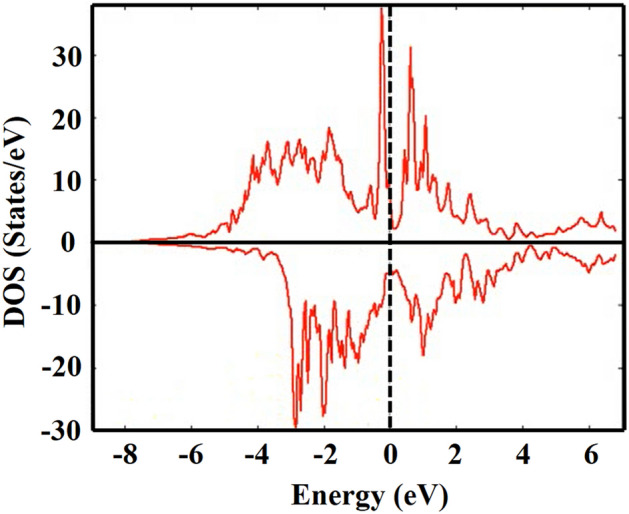
The spin-up and spin-down electronic density of states (DOS) for YFe₃.

Figure 2.

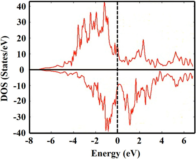
The spin-up and spin-down electronic density of states (DOS) for HoFe₃.

The total DOS, at ${\text{E}}_{\text{f}}$ for these two compounds are 10.915 and 24.461 states/eV, respectively. Therefore the electronic heat capacity coefficients, as calculated from Eq. 26, are 0.0256 and 0.0575 J/mol. K² respectively. The DOS of both compounds show that these two systems are metallic with fairly large density of states, at Fermi energy, in both the spin up and spin down configuration. This, of course, demands taking the electronic contribution to the heat capacity into consideration as we pointed out (Eq. 26).

Magnetization

Using the two-sublattice molecular field theory, the temperature dependence of magnetization of the rare earth and Fe sublattices, as well as total magnetization for ${\mathrm{YFe}}_3$ and ${\mathrm{HoFe}}_3$, are calculated. Total magnetic moments for ${\mathrm{YFe}}_3$ and ${\mathrm{HoFe}}_3$ ,calculated using the ab initio method are 4.8 µ_B/f.u and 4.4 µ_B /f.u, respectively, which are in good agreement with available experimental values, i.e. 4.88 and 4.59 µ_B /f.u as reported by J. F. Herbst et al.²². Table 1 displays the magnetic moments calculated in the present work and those by Ref.²². Figures 3 and 4a display mean-field- calculated temperature-dependence of magnetization, in zero field for ${\mathrm{YFe}}_3$ and ${\mathrm{HoFe}}_3\mathrm{respectively}$. The total magnetic moments of these two compounds, at very low temperatures, are in excellent agreement with the values referred to in Table 1. In addition we displayed, in Figs. 3 and 4b, both our mean field calculated magnetization and the experimental data extracted from Ref.²².

Table 1.

Magnetic moments at very low temperature (~ 0 K) using our calculation, in comparison to experimental data.

Method	YFe3 (µB)	HoFe3 (µB)	Reference
Ab initio	4.8	4.4	Present work
Experimental	4.88	4.59	22
Mean-field	4.8	4.6	Present work

Figure 3.

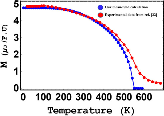
Total magnetization of YFe₃ in zero field vs. temperature.

Figure 4.

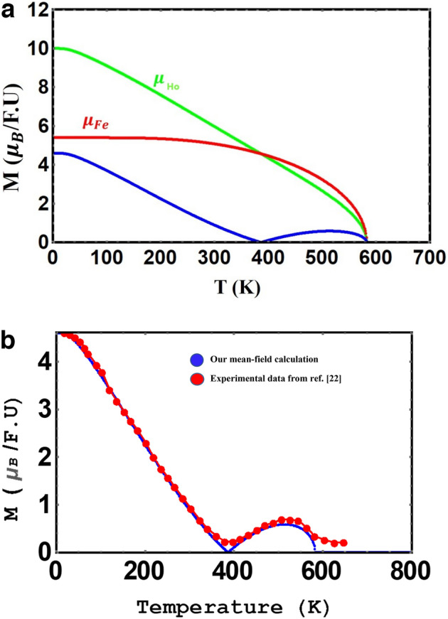
(a) Mean-field calculated total and sublattice magnetization of HoFe₃, in zero field, vs. temperature. (b) Total magnetization of HoFe₃ vs. temperature.

Ferromagnetic order for YFe₃ is evident from Fig. 3 and the magnetic moment per Fe atom is about 1.6 µ_B in agreement with the value in Fig. 1 in Herbst work²². On the other hand, a ferrimagnetic order with a compensation point is found for HoFe₃. As the magnetic moments of the Fe and Ho sublattices become equal and antiparallel, a cancellation of the total moment takes place close to 400 K. The continuous decrease in magnetization at Tc is a well-known feature of SOPT materials⁵⁴.

The temperature dependence of the magnetization, in 1, 3, 5 and 7 T fields, for ${\mathrm{HoFe}}_3$, is shown in Fig. 5. an increase in the Curie temperature and a decrease in the compensation temperature is evident, with increasing the field. This behavior is consistent with that found in ferrimagnetic compounds, as reported for example, by P. von Ranke⁵⁵. We may notice that even as the field increases the magnetization still has a continuous drop at Tc. Again, this confirms the SOPT nature of the studied compounds.

Figure 5.

Total magnetization of HoFe₃ in different applied fields 1, 3, 5 and 7 T vs. temperature.

Heat capacity and entropy

As previously stated, three contributions must be calculated to determine the total heat capacity of these materials. Figures 6 and 7 show, respectively, the magnetic heat capacity for ${\mathrm{YFe}}_3$ and ${\mathrm{HoFe}}_3$ in different applied fields. The features of these two figures, at the Curie temperature, show that the transition is a second order phase transition. In contrast, in the FOPT case, the peak in the heat capacity shifts to higher temperatures as the field increases⁵³.

Figure 6.

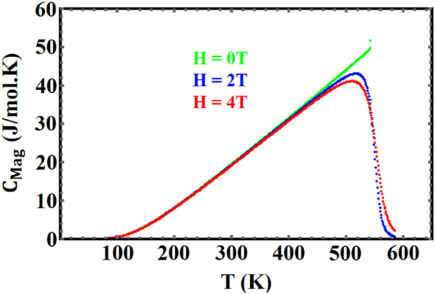
Magnetic heat capacity of ${\mathrm{YFe}}_3$ , in different fields, vs. temperature.

Figure 7.

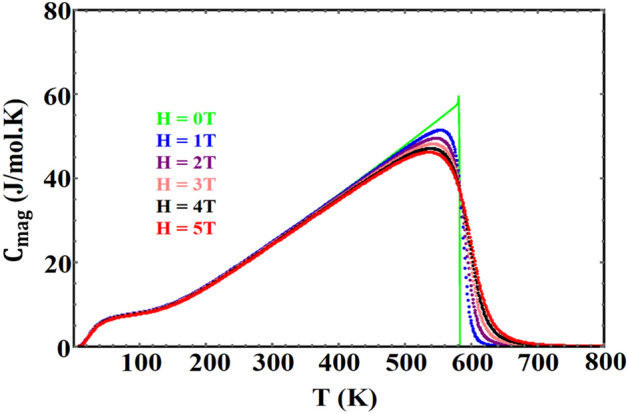
Magnetic heat capacity of HoFe₃ in different fields, vs. temperature.

The calculated magnetic entropy, in fields in the range 0–6 T, is shown in Figs. 8 and 9 for YFe₃ and HoFe₃ respectively. The entropy saturates to its maximum at T_c and above, and is reduced by increasing the field. The maximum values of the calculated magnetic entropy are about 27.3 and 50.9 J/mol. K for YFe₃ and HoFe₃, respectively. These values are calculated using the equation:

$${\text{S}}_{\text{max}}=\text{R}\left[ln\left(2{\text{J}}_{\text{r}}+1\right)+3ln\left(2{\text{J}}_{\text{Fe}}+1\right)\right],$$

where J_r and J_Fe are the total angular momenta for the rare earth and Fe atoms, respectively. The molecular-field results of the maximum magnetic entropy is in very good agreement with the results of the equation shown above. The gradual increase of the magnetic entropy with temperature until it saturates at T ≥ T_c instead of the sudden increase found in FOPT materials show that the transition in these two compounds is a SOPT one.

Figure 8.

The calculated magnetic entropy of ${\mathrm{YFe}}_3$ in two different fields vs. temperature.

Figure 9.

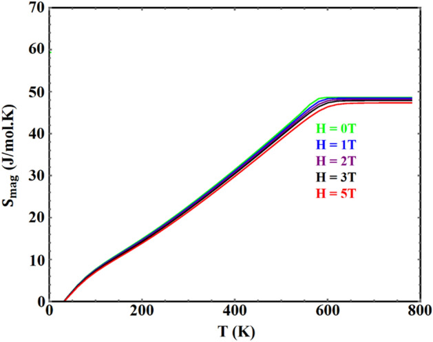
The calculated magnetic entropy of ${\mathrm{HoFe}}_3$ in different fields vs. temperature.

Elastic properties of $\mathbf{Y}{\mathbf{F}\mathbf{e}}_3$

The elastic properties of YFe₃ are calculated by using IRelast Package as available in the Wien2k Package⁴⁷, the output of the program is shown in Table 2.

Table 2.

The Elastic properties of YFe₃ as obtained from IRelast Package.

a. C11, C12, C13, C33, and C55 are the five independent elastic constants for a hexagonal symmetry as calculated from IRelast Package
Final elastic constants of YFe3 for a volume = 2466.7026 (Bohr radius)3
C11 = 195.3216 GPa C12 = 27.0896 GPa C13 = 61.1885 GPa C33 = 210.5720 GPa C55 = 149.9924 GPa

b. The bulk, shear, and Young modulus along with the Poisson’s coefficient as calculated from IRelast package
	VOIGT model Prediction	REUSS model Prediction	HILL model Prediction
Bulk modulus	100.016 (GPa)	98.659 (GPa)	99.337 (GPa)
Shear modulus	106.936 (GPa)	95.487 (GPa)	101.211 (GPa)
Young modulus	236.514 (GPa)	216.586 (GPa)	226.655 (GPa)
Poisson's coefficient	0.105	0.134	0.119

c. Transverse, longitudinal, and average elastic sound wave velocity along with the Debye temperature as calculated from IRelast package
By using HILL data: Transverse elastic wave velocity = 3805.19 (m/s) Longitudinal elastic wave velocity = 5789.42 (m/s) The average wave velocity = 4167.31 (m/s)	Debye temperature = 500.5(K)

The Debye temperature is calculated from the mean sound velocity. The bulk and shear moduli of ${\mathrm{YFe}}_3$, using the Hill model, are 99.337 and 101.211 GPa, respectively. The calculated ${\theta }_D$ for ${\mathrm{YFe}}_3$ is 500.5 K. For the HoFe₃ compound, the Debye temperature is 357.85 as reported by the Materials Project site (Kristin Persson)³².

Magnetocaloric effect

Isothermal entropy change

Figures 10 and 11 show the isothermal entropy change, for different magnetic fields, for ${\mathrm{YFe}}_3$ and ${\mathrm{HoFe}}_3$ respectively. The $\mathrm{\Delta }\mathrm{Sm}$ curve for ${\mathrm{HoFe}}_3$ exhibits two peaks: the first is a broad peak below the compensation temperature, and the second, smaller peak, has its maximum at the ferrimagnetic-paramagnetic phase transition at $T_C=590K$. These two features correspond to the inverse and direct MCE effects, respectively. For ferromagnetic ${\mathrm{YFe}}_3$ there is only one peak at a temperature around its T_c (545 K). The temperature and field dependences of ∆S_m are those of SOPT materials. In particular, the curves at different fields have their maxima at Tc. In FOPT materials, the peak shifts to higher temperatures as the field increases⁵³.

Figure 10.

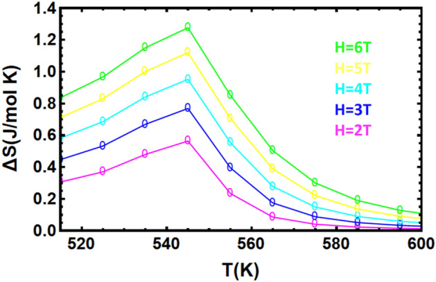
Temperature dependence of isothermal change in entropy for YFe₃ in fields: 2, 3, 4, 5 and 6 T.

Figure 11.

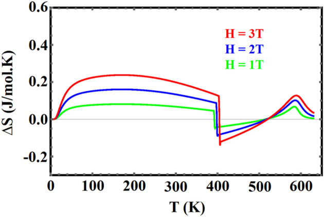
Temperature dependence of isothermal change in entropy for HoFe₃ in fields of 1, 2 and 3 T.

Adiabatic change in temperature

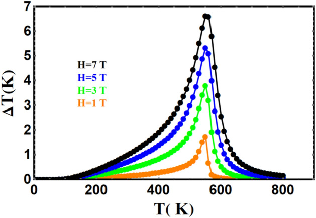
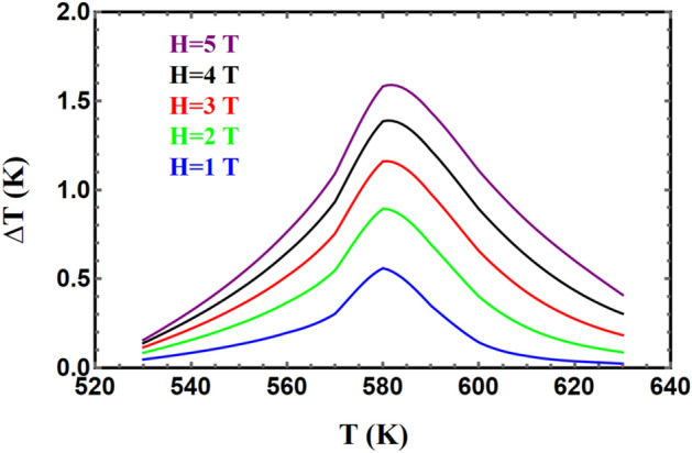
We have calculated the adiabatic change in temperature for different field changes, as shown in Figs. 12 and 13, for YFe₃ and HoFe₃ systems, respectively. It is clear that the former compound has a higher cooling rate than the latter in agreement with reported literature⁵⁶. For example, cooling rates about 1.3 and 0.4 K/T are achieved for these two compounds respectively for a field change of 3 T. The curves in each of Figs. 12 and 13 have their maxima centred at the Curie temperature. This is a known feature of compounds exhibiting second order phase transition and treated via the mean-field theory⁵³.

Figure 12.

The field-dependence of the adiabatic change in temperature vs. temperature for ${\mathrm{YFe}}_3$.

Figure 13.

The field-dependence of the adiabatic change in temperature vs. temperature for ${\mathrm{HoFe}}_3.$

The relative cooling power RCP (T)

The RCP is a figure-of-merit for MCE materials (e.g.⁵⁶). It is defined as RCP (T) = ∆T_ad (max) × δT_FWHM. Table 3 displays the RCP (T) for benchmark materials e.g. Gd, Gd-based compounds and FeRh system. From this data, we may conclude that the RCP of YFe₃ is comparable with those of well-known materials.

Table 3.

The Relative Cooling Power RCP (T), using our calculation, in comparison to experimental data.

Material	∆H(T)	RCP(T)/∆H (K2/T)	Reference
Gd	6	161.2	56
Fe	3	95
Co	2.32	78.4
Gd5Ge4	5	50.4
Gd5Si4	5	109
Gd 0.2 Er 0.8 Ni Al	5	75.9
FeRh	2.5	−66.4
YFe3	1.58	34.2
HoFe3	1.58	3.5
YFe3	3	85	Present work
HoFe3	3	15	Present work

The Arrott plots and universal curve

The Arrott plots for YFe₃ are shown, in a temperature range around T_c, in Fig. 14. The positive slopes at those temperatures, below and above T_c, are indicative of second order phase transition. First order transitions exhibit negative or s-shaped slopes^57,58. The straight line starting near the origin is calculated at a temperature close to Tc (Fig. 3). The features of the universal curve, described below, supports the presence of SOPT as well.

Figure 14.

The Arrott plots, at different temperatures, for YFe₃.

The universal curves⁵⁹, for YFe₃, are shown in Fig. 15 for field changes of 3, 4, 5 and 6 T. The curves are collapsed on each other especially at high temperatures i.e. θ > 0. The parameter θ is given by: θ = (T − T_c) / (T_r − T_c), where T_r is a reference temperature defined as the temperature at which the following condition holds: ∆S_M (T_r) = 0.7 (∆S_M)^peak. The collapse of the ΔS_M curves is also indicative of second order phase transition, which is different from the features encountered in first order phase transitions⁶⁰.

Figure 15.

The universal curve for YFe₃.

It would be of interest to support our finding that the mean field theory is suitable for explaining the physical properties. Therefore, calculating some of the critical exponents^61–65 would be beneficial. We have calculated the exponent n in the relation:

$$\mathrm{\Delta }{S}_m\sim H^n$$

from the field dependence of ΔS_m close to T_c. The relation between n, β and γ is:

n = 1 + (β−1)/(β + γ) [e.g. ⁶⁵, which can be used to evaluate γ if β is calculated from the relation:

$$M\sim {\left(-t\right)}^{\beta }H=0,T<T_c$$

or calculate β, if γ is calculated from:${\chi }_T\sim t^{-\gamma },H=0,T>T_c$, where t = (T−T_c)/T. We have calculated β for YFe₃ from its M-T data, in zero field, by taking the logarithm of M ~ (−t)^β and performing the calculation for temperatures lower than T_c. We have obtained β around 0.52 for this compound. Therefore, the percentage error between our result and the value 0.5 of the mean-field is around 4%. The factor γ turned out to be around 0.92 for YFe₃. In addition, we have calculated the critical exponent δ from the relation: δ = 1 + γ/β⁶⁶ and found that δ = 2.8, which is close to the MFT value of 3. From the above analysis, we conclude that mean-field theory has fairly produced the critical exponents for YFe₃. We would also emphasize the fact that the mean-field theory has its own limitations near T_c.

We should mention that other models e.g. 3D-Heisnberg, 3D- Ising and Tri-critical mean field model [e.g.⁶⁷] may be used to study the critical exponents, however a future experimental and/or theoretical work, dedicated to this task, may shed more light on the most proper model.

Conclusions

The two-sublattice molecular field model was used for calculating the thermomagnetic properties for ${\mathrm{YFe}}_3$ and ${\mathrm{HoFe}}_3$. The temperature dependence of magnetization shows that ${\mathrm{YFe}}_3$ is ferromagnetic with a Curie temperature close to 537 K, while ${\mathrm{HoFe}}_3$ is a ferrimagnetic compound with a compensation point around 389 K and a Curie temperature close to 565 K. The bulk and shear moduli are calculated using the WIEN2K ab-initio electronic code for YFe₃ system. Those moduli were used to calculate its Debye temperature (500.53 K). The Debye temperature of HoFe₃ is obtained from the Materials Project site. Using the calculated DOS, at Fermi energy, the electronic heat capacity coefficient ${\gamma }_e$ was found to be 0.0256 and 0.0575 J/$K^2$ mole, for ${\mathrm{YFe}}_3$ and ${\mathrm{HoFe}}_3$ respectively. The isothermal change in entropy ∆S_m, for a field change of 3 T, is about 0.8 and 0.12 J/mole. K for these systems, respectively. The Y-system exhibits a larger adiabatic drop in temperature (1.3 K/T), for a 3 T field change, than the Ho-system (0.4 K/T). The relative cooling power RCP(T) of YFe₃ is comparable to well-known MCE materials The temperature and field dependences of the magnetization, magnetic heat capacity, entropy, the MCE quantities together with the Arrott plots and universal curve, are all indicative of SOPT.

Author contributions

M.S.M.A.-E.: Performing the ab initio calculation, writing, reviewing. T.H.: Reviewing calculation and manuscript. A.A.- K.: Assisted in carrying out the MCE calculation using Mathematica, preparing figures. N.E.-S.: Carrying out the trapezoidal calculation, reviewing the manuscript. S.Y.: reviewing all the calculation, writing the original manuscript. SH.A.: Suggesting the systems to work on, reviewing the calculation and the original manuscript. F.Z.M.: performing the magnetocaloric calculation using Mathematica, reviewing the ab initio calculation, reading the manuscript.

Funding

Open access funding provided by The Science, Technology & Innovation Funding Authority (STDF) in cooperation with The Egyptian Knowledge Bank (EKB). The research leading to these results received funding from [ASRT, Egypt] under Grant Agreement No [6701]. ASRT is the second affiliation of this research.

Data availability

The datasets generated and/or analyzed during the current study are available from the corresponding author on reasonable request.

Competing interests

The authors declare no competing interests.

References

- 1.- Tishin, A. M. Handbook of Magnetic Materials, edited by KHJ Buschow North Holland. In Chapter 4: Magnetocaloric Effect in the Vicinity of Phase Transitions, 395–524. 10.1016/S1567-2719(99)12008-0 (1999).
- 2.Pecharsky VK, Gschneidner Jr KA. Magnetocaloric effect and magnetic refrigeration. J. Magn. Magn. Mater. 1999;200(1–3):44–56. doi: 10.1016/S0304-8853(99)00397-2. [DOI] [Google Scholar]
- 3.O'Keefe TJ, Roe GJ, James WJ. X-ray investigation of the iron-holmium system. J. Less Common Metals. 1968;15(3):357–360. doi: 10.1016/0022-5088(68)90196-3. [DOI] [Google Scholar]
- 4.Tharp DE, Long GJ, Pringle OA, James WJ, Grandjean F. A Mössbauer effect study of ErFe3. J. Magn. Magn. Mater. 1992;104–107:1477–1478. doi: 10.1016/0304-8853(92)90670-J. [DOI] [Google Scholar]
- 5.Ray A, Strnat K. Easy directions of magnetization in ternary R2 (Co, Fe)17 phases. IEEE Trans. Magn. 1972;8(3):516–518. doi: 10.1109/TMAG.1972.1067471. [DOI] [Google Scholar]
- 6.Ross JW, Crangle J. Magnetization of cubic laves phase compounds of rare earths with cobalt. Phys. Rev. 1964;133(2A):509–510. doi: 10.1103/PhysRev.133.A509. [DOI] [Google Scholar]
- 7.Wertheim GK, Wernick JH. Mössbauer effect in some iron-rare Earth intermetallic compounds. Phys. Rev. 1962;125(6):1937. doi: 10.1103/PhysRev.125.1937. [DOI] [Google Scholar]
- 8.Marei SA, Craig RS, Wallace WE, Tsuchida T. Magnetic characteristics of some Laves phase systems containing Fe and Mn. J. Less Common Metals. 1967;13(4):391–398. doi: 10.1016/0022-5088(67)90033-1. [DOI] [Google Scholar]
- 9.- Wallace. W. E., Skrabek, E. A. In Rare Earth Research Volume 2, Proceedings of the Third Rare Earth Conference, edited by K. S. Vorres (Gordon and Breech, New York, 1964), p. 417. 431.
- 10.- Roe, G. J. The iron-holmium binary system and related magnetic properties. "Doctoral Dissertations". 1876. https://scholarsmine.mst.edu/doctoral_dissertations/1876 (1969).
- 11.- Hoffer. G. I., Salmans, L. R. 7th Rare Earth Research Conf. Cornado, California 371 (1968).
- 12.Földeàki M, Chahine R, Bose TK. Magnetic measurements: a powerful tool in magnetic refrigerator design. J. Appl. Phys. 1995;77(7):3528–3537. doi: 10.1063/1.358648. [DOI] [Google Scholar]
- 13.Li L, Yan M. Recent progresses in exploring the rare earth based intermetallic compounds for cryogenic magnetic refrigeration. J. Alloys Compd. 2020;823:153810. doi: 10.1016/j.jallcom.2020.15381. [DOI] [Google Scholar]
- 14.Zhang Y. Review of the structural, magnetic and magnetocaloric properties in ternary rare earth RE2T2X type intermetallic compounds. J. Alloy. Compd. 2019;787:1173–1186. doi: 10.1016/j.jallcom.2019.02.175. [DOI] [Google Scholar]
- 15.De Oliveira, N. A., von Ranke, P. J. Theoretical aspects of the magnetocaloric effect. Phys. Rep. 489(4–5), 89–159. doi:10.1016/j.physrep.2009.12.006 (2010).
- 16.Nikitin SA, Talalaeva EV, Chernikova LA, Andreenko AS. Magnetocaloric effect in compounds of rare-earth metals with iron. Soviet J. Exp. Theor. Phys. 1974;38:1028. [Google Scholar]
- 17.Nagy A, Hammad T, Yehia S, Aly SH. Thermomagnetic properties and magnetocaloric effect of TmFe2 compound. J. Magn. Magn. Mater. 2019;473:324–330. doi: 10.1016/j.jmmm.2018.10.050. [DOI] [Google Scholar]
- 18.Tian G, Dua H, Zhanga Y, Xiaa Y, Wanga C, Han J, Liu S, Yang J. Large reversible magnetocaloric effect of light rare-earth intermetallic compound Pr5Si3. J. Alloy. Compd. 2010;496:517–520. doi: 10.1016/j.jallcom.2010.02.093. [DOI] [Google Scholar]
- 19.Clark AE. Magneto-strictive rare earth-Fe2 compounds. Handb. Ferromagn. Mater. 1980;1:531–589. doi: 10.1016/S1574-9304(05)80122-1. [DOI] [Google Scholar]
- 20.Campbell IA. Indirect exchange for rare earths in metals. J. Phys. F: Met. Phys. 1972;2(3):L47. doi: 10.1088/0305-4608/2/3/004. [DOI] [Google Scholar]
- 21.Craig RS, Wallace WE, Kevin-Smith H. Hydrogenation of intermetallic compounds: thermodynamic aspects. Sci. Technol. Rare Earth Mater. 1980;55:353. doi: 10.1016/B978-0-12-675640-1.50021-0. [DOI] [Google Scholar]
- 22.Herbst JF, Croat JJ. Magnetization of RFe3 intermetallic compounds: molecular field theory analysis. J. Appl. Phys. 1982;53(6):4304–4308. doi: 10.1063/1.331207. [DOI] [Google Scholar]
- 23.Herbst JF, Croat JJ. Magnetization of R6Fe23 intermetallic compounds: molecular field theory analysis. J. Appl. Phys. 1984;55(8):3023–3027. doi: 10.1063/1.333293. [DOI] [Google Scholar]
- 24.Aly SH, Yehia S. A computer simulation study on a two-sublattice magnetic system. J. Magn. Magn. Mater. 2000;213(3):383–388. doi: 10.1016/s0304-8853(99)00805-7. [DOI] [Google Scholar]
- 25.Shafiq M, Ahmad I, Jalali-Asadabadi S. Theoretical studies of strongly correlated rare-earth intermetallics RIn3 and RSn3 (R= Sm, Eu, and Gd) J. Appl. Phys. 2014;116(10):103905. doi: 10.1063/1.4894833. [DOI] [Google Scholar]
- 26.Blaha P, Schwarz K, Tran F, Laskowski R, Madsen GKH, Marks LD. WIEN2k: An APW+lo program for calculating the properties of solids. J. Chem. Phys. 2020;152:074101. doi: 10.1063/1.5143061. [DOI] [PubMed] [Google Scholar]
- 27.Debye P. Zurtheorie der spezifischenwärmen. Ann. Phys. 1912;344(14):789–839. doi: 10.1002/andp.19123441404. [DOI] [Google Scholar]
- 28.- Kittel, C. Elementary Statistical Physics. Courier Corporation (2004).
- 29.Kittel, C., McEuen, P. (1996) Introduction to Solid State Physics, vol. 8. New York: Wiley.
- 30.Andersen OK. Linear methods in band theory. Phys. Rev. B. 1975;12(8):3060. doi: 10.1103/PhysRevB.12.3060. [DOI] [Google Scholar]
- 31.Stadler R, Wolf W, Podloucky R, Kresse G, Furthmüller J, Hafner J. Ab initio calculations of the cohesive, elastic, and dynamical properties of CoSi2 by pseudopotential and all-electron techniques. Phys. Rev. B. 1996;54:1729. doi: 10.1103/PhysRevB.54.1729. [DOI] [PubMed] [Google Scholar]
- 32.- Persson, K. A. https://materialsproject.org/
- 33.Kohn W, Sham LJ. Self-consistent equations including exchange and correlation effects. Phys. Rev. 1965;140(4A):A1133. doi: 10.1103/PhysRev.140.A1133. [DOI] [Google Scholar]
- 34.- Singh, D. J., Nordstrom, L. Planewaves, Pseudopotentials, and the LAPW method, 2nd Edition. Springer (2006).
- 35.Perdew JP, Wang Y. Accurate and simple analytic representation of the electron-gas correlation energy. Phys. Rev. B. 1992;45(23):13244. doi: 10.1103/PhysRevB.45.13244. [DOI] [PubMed] [Google Scholar]
- 36.Perdew JP, Burke K, Ernzerhof M. Generalized gradient approximation made simple. Phys. Rev. Lett. 1996;77(18):3865. doi: 10.1103/PhysRevLett.77.3865. [DOI] [PubMed] [Google Scholar]
- 37.Singh DJ. Ground-state properties of lanthanum: Treatment of extended-core states. Phys. Rev. B. 1991;34(8):6388. doi: 10.1103/PhysRevB.43.6388. [DOI] [PubMed] [Google Scholar]
- 38.Mohammad FA, Yehia S, Aly SH. A first-principle study of the magnetic, electronic and elastic properties of the hypothetical YFe5 compound. Physica B: Condens. Matter. 2012;407(13):2486–2489. doi: 10.1016/j.physb.2012.03.050. [DOI] [Google Scholar]
- 39.Shabara RM, Aly SH. A first-principles study of elastic, magnetic, and structural properties of PrX2 (X=Fe, Mn, Co) compounds. J. Magn. Magn. Mater. 2017;423:447–452. doi: 10.1016/j.jmmm.2016.09.075. [DOI] [Google Scholar]
- 40.Aly SH, Shabara RM. First principles calculation of elastic and magnetic properties of Cr-based full-Heusler alloys. J. Magn. Magn. Mater. 2014;360:143–147. doi: 10.1016/j.jmmm.2014.02.030. [DOI] [Google Scholar]
- 41.Elalfy GM, Shabara RM, Aly SH, Yehia S. First-principles study of magnetic, electronic, elastic and thermal properties of GdFe2.". Comput. Condens. Matter. 2015;5:24–29. doi: 10.1016/j.cocom.2015.10.001. [DOI] [Google Scholar]
- 42.Habbak EL, Shabara RM, Aly SH, Yehia S. Investigating half-metallicity in PtXSb alloys (X=V, Mn, Cr, Co) at ambient and high pressure. Physica B: Condens. Matter. 2016;494:63–70. doi: 10.1016/j.physb.2016.04.009. [DOI] [Google Scholar]
- 43.Shabara RM, Yehia S, Aly SH. Pressure-induced phase transitions, electronic and magnetic properties of GdN. Results Phys. 2011;1:30–35. doi: 10.1016/j.rinp.2011.08.001. [DOI] [Google Scholar]
- 44.Abu-Elmagd MSM, Aly SH, Yehia S. Magnetic properties and electronic structure of TℎCo4B. Model. Numer. Simul. Mater. Sci. 2012;2(3):51–59. doi: 10.4236/mnsms.2012.23006. [DOI] [Google Scholar]
- 45.Yehia S, Aly SH, Aly AE. Electronic band structure and spin-density maps of SmCo5. Comput. Mater. Sci. 2008;41(4):482–485. doi: 10.1016/j.commatsci.2007.05.004. [DOI] [Google Scholar]
- 46.Jamal M, Kamali Sarvestani N, Yazdani A, Reshak AH. Mechanical and thermodynamical properties of hexagonal compounds at optimized lattice parameters from two-dimensional search of the equation of state. RSC Adv. 2014;4(101):57903–57915. doi: 10.1039/C4RA09358E. [DOI] [Google Scholar]
- 47.Jamal M, Bilal M, Ahmad I, Jalali-Asadabadi S. IRelast package. J. Alloy. Compd. 2018;735:569–579. doi: 10.1016/j.jallcom.2017.10.139. [DOI] [Google Scholar]
- 48.- Jamal, M. IRelast. http://www.wien2k.at/ (2019).
- 49.Foster AS, Sulimov VB, Lopez Gejo F, Shluger AL, Nieminen RM. Structure and electrical levels of point defects in monoclinic zirconia. Phys. Rev. B. 2001;64(22):224108. doi: 10.1103/PhysRevB.64.224108. [DOI] [Google Scholar]
- 50.Anderson OL. A simplified method for calculating the Debye temperature from elastic constants. J. Phys. Chem. Solids. 1963;24(7):909–917. doi: 10.1016/0022-3697(63)90067-2. [DOI] [Google Scholar]
- 51.- Schreiber, E., Anderson, O. L., Soga, N., Bell, J. F. Elastic constants and their measurement, 747–748. 10.1115/1.3423687(1975).
- 52.Morrish, A. H. The Physical Principles of Magnetism. New York: Wiley. 10.1002/9780470546581 (2001).
- 53.Smith A, Bahl CRH, Bjørk R, Engelbrecht K, Nielsen KK, Pryds N. Materials challenges for high performance magnetocaloric refrigeration devices. Adv. Energy Mater. 2012;2(11):1288–1318. doi: 10.1002/aenm.201200167. [DOI] [Google Scholar]
- 54.Lyubina J. Magnetocaloric materials for energy efficient cooling. J. Phys. D: Appl. Phys. 2017;50:053002. doi: 10.1088/1361-6463/50/5/053002. [DOI] [Google Scholar]
- 55.Von Ranke PJ, Alho BP, Nobrega EP, de Oliveira NA. Understanding the inverse magnetocaloric effect through a simple theoretical model. Physica B. 2009;404(19):3045–3047. doi: 10.1016/j.physb.2009.07.009. [DOI] [Google Scholar]
- 56.- Gschneidner Jr., K. A., Pecharsky, V. K. Intermetallic Compounds: Principles and Practice Vol. 3, Ch.25, Wiley. 10.1002/0470845856.ch25 (2002).
- 57.Law JY, Franco V, Moreno-Ramírez LM, Conde A, Karpenkov DY, Radulov I, Skokov KP, Gutfleisch O. A quantitative criterion for determining the order of magnetic phase transitions using the magnetocaloric effect. Nat. Commun. 2018;9(1):1–9. doi: 10.1038/s41467-018-05111-w. [DOI] [PMC free article] [PubMed] [Google Scholar]
- 58.Foldeaki M, Schnelle W, Gmelin E, Benard P, Koszegi B, Giguere A, Chahine R, Bose TK. Comparison of magnetocaloric properties from magnetic and thermal measurements. J. Appl. Phys. 1997;82(1):309–316. doi: 10.1063/1.365813. [DOI] [Google Scholar]
- 59.Franco V, Conde A. Scaling laws for the magnetocaloric effect in second order phase transitions: from physics to applications for the characterization of materials. Int. J. Refrig. 2010;33(3):465–473. doi: 10.1016/j.ijrefrig.2009.12.019. [DOI] [Google Scholar]
- 60.Bonilla CM, Herrero-Albillos J, Bartolomé F, García LM, Parra-Borderías M, Franco V. Universal behavior for magnetic entropy change in magnetocaloric materials: an analysis on the nature of phase transitions. Phys. Rev. B. 2010;81(22):224424. doi: 10.1103/PhysRevB.81.224424. [DOI] [Google Scholar]
- 61.Magnetic critical scattering, Malcolm F. Collins, Theory of critical phenomena: critical exponents, table 3.1 on p. 12 (Oxford University Press, 1989).
- 62.- Long Range Order in Solids, Robert M. White, and Theodore H. Geballe, ch.1: Phase transitions and order parameters (Academic Press, 1979).
- 63.- Magnetism in the Solid State: an introduction, Peter Mohn, ch.5, Springer 2006.
- 64.- Quantitative Theory of Critical Phenomena, George A. Baker, Jr. ch.1 (Academic press 1990).
- 65.El Ouahbi A, Yamkane Z, Derkaoui S, Lassri H. Magnetic properties and the critical exponents in terms of the magnetocaloric effect of amorphous Fe40Ni38Mo4B18 alloy. J. Superconductivity Novel Magn. 2021;34:1253. doi: 10.1007/s10948-021-05832-y. [DOI] [Google Scholar]
- 66.Widom B. "Equation of state in the neighborhood of the critical point. J. Chem. Phys. 1965;43:3898. doi: 10.1063/1.1696618. [DOI] [Google Scholar]
- 67.Bally MAA, Islam MA, Hoque SM, Rashid R, Islam MdF, Khan FA. Magnetocaloric properties and analysis of the critical point exponents at PM-FM phase transition. Results Phys. 2021;28:104546. doi: 10.1016/j.rinp.2021.104546. [DOI] [Google Scholar]
Associated Data
This section collects any data citations, data availability statements, or supplementary materials included in this article.
Data Availability Statement