Preference Matrix Guided Sparse Canonical Correlation Analysis for Genetic Study of Quantitative Traits in Alzheimer’s Disease

Abstract

Investigating the relationship between genetic variation and phenotypic traits is a key issue in quantitative genetics. Specifically for Alzheimer’s disease, the association between genetic markers and quantitative traits remains vague while, once identified, will provide valuable guidance for the study and development of genetic-based treatment approaches. Currently, to analyze the association of two modalities, sparse canonical correlation analysis (SCCA) is commonly used to compute one sparse linear combination of the variable features for each modality, giving a pair of linear combination vectors in total that maximizes the cross-correlation between the analyzed modalities. One drawback of the plain SCCA model is that the existing findings and knowledge cannot be integrated into the model as priors to help extract interesting correlation as well as identify biologically meaningful genetic and phenotypic markers. To bridge this gap, we introduce preference matrix guided SCCA (PM-SCCA) that not only takes priors encoded as a preference matrix but also maintains computational simplicity. A simulation study and a real-data experiment are conducted to investigate the effectiveness of the model. Both experiments demonstrate that the proposed PM-SCCA model can capture not only genotype-phenotype correlation but also relevant features effectively.

I. Introduction

Investigating the relationship between genetic variation and phenotypic traits is a key issue in quantitative genetics. Specifically for Alzheimer’s disease, the association between genetic markers and quantitative traits (e.g., molecular, imaging and cognitive measures) remains vague while, once identified, will provide valuable guidance for the study and development of genetics-based treatment approaches. However, considering the vast number of genetic markers such as single nucleotide polymorphisms (SNPs) and multimodal quantitative traits (QTs), it would be computationally expensive and less powerful to perform univariate testing on all possible SNP-QT pairs. Therefore, as an alternative method, canonical correlation analysis (CCA) is commonly used to detect multi-SNP-multi-QT associations between genotype and quantitative phenotype data in a single model [1]–[5]. A plain CCA computes two canonical weight vectors for each modality as linear combinations of feature variables in two modalities that maximize their cross-correlation. Despite all the advantages of CCA, its result is usually not informative: on one hand, the dimensions of SNP and QT datasets are usually extremely high, allowing infinitely many solutions to exist; on the other hand, the low signal-to-noise ratio in most SNP and QT datasets is directly reflected in the result weight vectors, thereby lowering the result interpretability in practice.

To counter these drawbacks, sparse CCA (SCCA) is later proposed to reduce the number of variables selected in the canonical weight vectors [6]. While the results by SCCA are much more robust and interpretable in practice, the direct computation of SCCA is expensive, which makes it challenging to perform analysis given limited computational resource. For computational efficiency, in practice, a simplified version of SCCA (equivalent to sparse partial least square regression or SPLS) is often widely used through maximizing the cross-covariance of two canonical variables [7]. This simplification makes some additional assumptions on the problem that SCCA solves but transforms the fractional optimization problem into a constrained optimization problem with closed-form solutions for each subproblem, which reduces the computational cost.

One common disadvantage of these models is that the existing findings from past biomedical research cannot be integrated into the procedure of these models as priors. Nonetheless, the priors about relations between SNPs and QTs are valuable in variable selection and will offer more practical meaning and interpretability in the result by SCCA. In this paper, we propose a new SCCA model, named as “preference matrix guided SCCA (PM-SCCA)”, which not only takes priors encoded as a preference matrix but also keeps computational simplicity by transforming it to the simplified SPLS version described above. The discussion about CCA models in the rest of the paper all refer to this simplified version. The preference matrix contains the numeric values of how preferred one SNP is deemed as associated with one QT as priors based on existing biological knowledge. A simulation study and a real-data experiment are conducted to investigate the effectiveness of the model. Both experiments demonstrate that the proposed PM-SCCA model is capable of capturing not only multi-SNP-multi-QT associations but also relevant genetic and phenotypic features effectively.

The rest of this paper is organized as follows. In Section II, we introduce the problem formation of the proposed PM-SCCA. In Section III, we explain the method to perform PM-SCCA and models’ performance in the simulation study. In Section IV, we discuss the real-data experiment and its results. In Section V, we conclude the paper.

II. Problem formulation

Let $X\in {ℝ}^{n\times p}$ be the genotyping SNP data and $Y\in {ℝ}^{n\times q}$ be the quantitative trait (QT) data (e.g., molecular, imaging, fluid and/or cognitive measures), where n, p and q are the numbers of participants, SNPs and QTs, respectively. Assume the features variables (i.e., columns) in X, Y have been centered at zeros.

Canonical correlation analysis (CCA) aims to find a linear combination of features in X and Y to maximize the correlation between Xu and Yv. Mathematically, it finds the canonical weight vectors u, v that satisfy:

$$\underset{u,v}{\text{maximize}}\frac{u^{\top }{X}^{\top }Yv}{\Vert Xu{\Vert }_2\Vert Yv{\Vert }_2}\equiv \underset{u,v}{\text{maximize}}\frac{u^{\top }{\Sigma }_{XYv}}{\sqrt{u^{\top }{\Sigma }_{XX}u{v}^{\top }{\Sigma }_{YYv}}}$$ (1)

It is customary to interpret Σ_XX and Σ_YY as diagonal matrices since the SNP and QT data typically exhibit both high dimensionality and insignificant correlation among features [8]–[10]. This simplification allows the fractional optimization problem to be reduced to a constrained optimization problem. Additionally, since sparsity on the loadings is desired for feature selection and practical interpretation in biological settings, we employ a simplified sparse CCA (SCCA), equivalent to sparse PLS (SPLS), for the following problem:

$$\begin{array}{ll}\underset{u,v}{\text{maximize}}\hfill & \frac{1}{n-1}{u}^{\top }{X}^{\top }Yv\hfill \\ \text{subject to }\hfill & \Vert u{\Vert }_2^2\le 1,\Vert u{\Vert }_1\le c_1\hfill \\ \hfill & \Vert v{\Vert }_2^2\le 1,\Vert v{\Vert }_1\le c_2\hfill \end{array}$$ (2)

where c₁, c₂ > 0 are the regularization parameters for sparsity and the objective function is often referred to as canonical covariance. In this paper, we introduce a new SCCA model, “preference matrix guided SCCA (PM-SCCA)”, and develop an algorithm based on the above computationally simplified model (i.e., Eq (2)). Thus PM-SCCA is formulated as

$$\begin{array}{ll}\underset{u,v}{\text{maximize}}\hfill & (1-\lambda )\cdot \frac{1}{n-1}{u}^{\top }{X}^{\top }Yv+\lambda \left|u{|}^{\top }E\right|v|\hfill \\ \text{subject to }\hfill & \Vert u{\Vert }_2^2\le 1,\Vert u{\Vert }_1\le c_1\hfill \\ \hfill & \Vert v{\Vert }_2^2\le 1,\Vert v{\Vert }_1\le c_2\hfill \end{array}$$ (3)

where c₁, c₂ > 0 and λ ∈ [0, 1) are the regularization parameters, E is the preference matrix with E_i,j ≥ 0 ∀i, j, and | · | stands for the elementwise absolute value. Each element in the preference matrix E reflects user-specified preference level (based on prior biological knowledge) on the corresponding SNP-QT association, and therefore regularizes the magnitude of the elements of both canonical weight vectors, u and v.

When c₁ = c₂ = +∞, the sparsity constraints will not be active. In this case, the methods are referred to as CCA and PM-CCA respectively. In our empirical study, we will compare the proposed PM-SCCA and PM-CCA with SCCA and CCA using both simulation and read world data.

III. Methods

We employ an alternating optimization method to solve Eq (2). Alternating optimization is an iterative procedure that proceeds in two alternating steps: update of u while holding v fixed and update of v while holding u fixed.

A. Update of u with v fixed

Denote

$$a=(1-\lambda )\cdot \frac{1}{n-1}{X}^{\top }Yv\in {ℝ}^{p\times 1},b=\lambda E\left|v\right|\in {ℝ}_{+}^{p\times 1}.$$

The optimization of Eq (3) with respect to u can be written as

$$\begin{array}{ll}\underset{u}{\text{maximize}}\hfill & {\sum }_{i=1}^p\left(a_i{u}_i+b_i\left|u_i\right|\right)\hfill \\ \text{subject to }\hfill & \Vert u{\Vert }_2^2\le 1,\Vert u{\Vert }_1\le c_1.\hfill \end{array}$$ (4)

Notice that, since b_i ≥ 0, it can be shown that the optimal u_i should have the same sign as a_i. Otherwise, by reversing the sign of u_i, the objective value can always be increased. Thus, with substitution |u_i| = sign (a_i) u_i, the following problem is equivalent to Eq (4):

$$\begin{array}{ll}\underset{u}{\text{maximize}}\hfill & {\sum }_{i=1}^p\left(a_i+b_i\text{sign}\left(a_i\right)\right)u_i\hfill \\ \text{subject to }\hfill & \Vert u{\Vert }_2^2\le 1,\Vert u{\Vert }_1\le c_1.\hfill \end{array}$$ (5)

With

$$w=\left(\begin{array}{c}{a}_1+b_1\text{sign}\left(a_1\right)\\ a_2+b_2\text{sign}\left(a_2\right)\\ ⋮\\ a_p+b_p\text{sign}\left(a_p\right)\end{array}\right).$$

defined, Eq (5) can be expressed in a more compact form as

$$\underset{u}{\text{maximize}}{w}^{\top }u\hspace{1em}\text{subject to}\Vert u{\Vert }_2^2\le 1,\Vert u{\Vert }_1\le c_1.$$ (6)

B. Update of v with u fixed

Solving v with u fixed is the same as solving u with v fixed. Specifically, denote

$$\alpha =(1-\lambda )\cdot \frac{1}{n-1}{Y}^{\top }Xu\in {ℝ}^{q\times 1},\beta =\lambda E^{\top }\left|u\right|\in {ℝ}_{+}^{q\times 1}$$

The optimization of Eq. (3) with respect to v can be written as

$$\begin{array}{ll}\underset{v}{\text{maximize}}\hfill & {\sum }_{j=1}^q\left({\alpha }_j{v}_j+{\beta }_j\left|v_j\right|\right)\hfill \\ \text{subject to }\hfill & \Vert v{\Vert }_2^2\le 1,\Vert v{\Vert }_1\le c_2.\hfill \end{array}$$ (7)

Since β_j ≥ 0, the optimal v_j should the same sign as α_j with the same reason as stated for u.

Define

$$\gamma =\left(\begin{array}{c}{\alpha }_1+{\beta }_1\text{sign}\left({\alpha }_1\right)\\ {\alpha }_2+{\beta }_2\text{sign}\left({\alpha }_2\right)\\ ⋮\\ {\alpha }_q+{\beta }_q\text{sign}\left({\alpha }_q\right)\end{array}\right).$$

Then, with similar techniques, the optimization problem to update v with u fixed can be boiled down to solving the following problems:

$$\underset{v}{\text{maximize}}{\gamma }^{\top }v\hspace{1em}\text{subject to }\Vert v{\Vert }_2^2\le 1,\Vert v{\Vert }_1\le c_2.$$ (8)

Let S(a, Λ) be the soft-thresholding operator:

$$S(a,\Lambda )=\{\begin{array}{ll}a-\Lambda ,\hfill & a>\Lambda \hfill \\ a+\Lambda ,\hfill & a<-\Lambda \hfill \\ 0,\hfill & -\Lambda \le a\le \Lambda \hfill \end{array}$$

where Λ is a non-negative constant. Note that the soft-thresholding operator with a constant parameter Λ and a vector input a can be computed component-wise.

The original Eq (3) has been reduced to two quadratically constrained linear programming optimization problems, Eq (6) and Eq (8). Notice that, with the ℓ₁ constraint, the solution is generally not unique with the nonzero elements possible to assume any non-negative number that satisfies the ℓ₁ constraint. Given an initial estimate for u and v, the algorithm for the PM-SCCA alternately updates u and v iteratively until convergence, as outlined in Algorithm 1. Note that Algorithm 1 calls a Quadratically Constrained Linear Programming (QCLP) Solver [11], which is outlined in Algorithm 2.

For soft-thresholding operator S(a, Λ₎ used in QCLP solver (outlined in Algorithm 2), the parameter Λ should be chosen flexibly. If ${\Vert \frac{S(a,\Lambda )}{\Vert S(a,\Lambda ){\Vert }_2}\Vert }_1\le c$, then choose Λ = 0. Otherwise, choose Λ according to the sparsity of the solution desired. Despite this common practice, we also allow Λ in Algorithm 2 to be an optional input, as Λ₁ and Λ₂ used in Algorithm 1, due to the possibility of tuning the parameter c faster and more accurately without using a prespecified parameter grid of c in certain cases.

Additionally, we see the preference matrix E as well-bounded if

$$\frac{\text{max}\left\{{\sigma }_{\text{min}}^{\prime }(X)\Vert Y{\Vert }_2,{\sigma }_{\text{min}}^{\prime }(Y)\Vert X{\Vert }_2\right\}}{n-1}\le \Vert E\Vert \le \frac{\Vert X{\Vert }_2\Vert Y{\Vert }_2}{n-1}$$

If E is not well-bounded, then it is advised to perform magnitude alignment as

$$E\leftarrow \{\begin{array}{cc}\frac{E{\Vert X^{\top }Y\Vert }_2}{(n-1)\Vert E{\Vert }_2}& (\text{A})\\ \frac{E\left(\Vert X{\Vert }_2\Vert Y{\Vert }_2+\text{max}\left\{{\sigma }_{\text{min}}^{\prime }(X)\Vert Y{\Vert }_2,{\sigma }_{\text{min}}^{\prime }(Y)\Vert X{\Vert }_2\right\}\right)}{2(n-1)\Vert E{\Vert }_2}& (\text{B})\end{array}$$

where (A) is when _X^⊤_Y can be computed and (B) is otherwise. (B) is considered because _X^⊤_Y is computationally expensive and approximations are sometimes required. Here, ${{\sigma }^{\prime }}_{\text{min}}$ (A) denotes the smallest non-trivial spectral radius of A. It is specifically defined this way because the matrix is easily ill-conditioned and the minimum spectral radius to be used can be filtered with a deliberately selected cutoff.

IV. Experimental results and discussions

A. Simulation study on synthetic data

We perform the simulation analyses to demonstrate that PM-SCCA can outperform SCCA in terms of prediction accuracy and CCA in terms of feature selection performance.

1). Generation of synthetic data:

We assume the data $X\in {ℝ}^{n_0\times p}$ and $Y\in {ℝ}^{n_0\times q}$ contain n₀ i.i.d. observations of random vectors $x\in {ℝ}^p$ and $y\in {ℝ}^q$ respectively, with n₀ = 2500, p = 200, and q = 100.

The probabilistic generative model for tensor CCA (TCCA) can be adapted by treating a matrix as a first-order tensor to generate synthetic data. The generative model for the first-order TCCA takes canonical weights u, v, the targeted canonical correlation ρ ≥ 0, the noise levels η_x ≥ 0, η_y ≥ 0, the means of the features μ_x, μ_y, and the number of observations n₀ to generate synthetic data [12]. The model adapted to our simulation study is described in detail as follows.

Given $u\in {ℝ}^p$ and $v\in {ℝ}^q$ specified as ground truth canonical weights for X and Y, we compute

$$\{\begin{array}{l}\tilde{u}=|\frac{u}{\Vert u{\Vert }_2^2}\hfill \\ \tilde{v}=\frac{v}{\Vert v{\Vert }_2^2}\hfill \end{array}\to \{\begin{array}{l}{\Sigma }_x=\tilde{u}{\tilde{u}}^{\top }+{\eta }_x\left(I_p-\Vert u{\Vert }_2^2\tilde{u}{\tilde{u}}^{\top }\right)\hfill \\ {\Sigma }_y=\tilde{v}{\tilde{v}}^{\top }+{\eta }_y\left(I_q-\Vert v{\Vert }_2^2\tilde{v}{\tilde{v}}^{\top }\right)\hfill \\ {\Sigma }_{xy}=\rho \tilde{u}{\tilde{v}}^{\top }\hfill \end{array}$$

Then, we generate X, Y by row-stacking n₀ draws from

$$\left[x_1,\dots ,x_p,y_1,\dots ,y_q\right]~𝓝\left(\left[{\mu }_x,{\mu }_y\right],\left[\begin{array}{cc}{\Sigma }_x& {\Sigma }_{xy}\\ {\Sigma }_{xy}^{\top }& {\Sigma }_y\end{array}\right]\right)$$

and separate the matrix as

$$[X\mid Y]=\left[\begin{array}{ccc}\hfill x_{1,1}\hfill & \hfill \dots \hfill & \hfill x_{1,p}\hfill \\ \hfill ⋮\hfill & \hfill \ddots \hfill & \hfill ⋮\hfill \\ \hfill x_{n_0,1}\hfill & \hfill \dots \hfill & \hfill x_{n_0,p}\hfill \end{array}|\begin{array}{ccc}\hfill y_{1,1}\hfill & \hfill \dots \hfill & \hfill y_{1,q}\hfill \\ \hfill ⋮\hfill & \hfill \ddots \hfill & \hfill ⋮\hfill \\ \hfill y_{n_0,1}\hfill & \hfill \dots \hfill & \hfill y_{n_0,q}\hfill \end{array}\right]$$

In our simulation study, we set the targeted canonical correlation as ρ = 0.3, the noise levels as η_x = η_y = 0.01 and the means of the features μ_x = 0p and μ_y = 0q.

We generate the preference matrix by, first, choosing which elements to be nonzero by random sampling and, then, drawing from a truncated normal $\psi \left({\mu }_E=1,{\sigma }_E^2={0.5}^2,0,+\infty \right)$ for the blocks between correlated features and the all other parts between uncorrelated feature respectively. As two weight groups in u and two weight groups in v are defined as non-trivial (Fig. 1, Theoretical), 2 × 2 = 4 nontrivial blocks in the covariance matrix of signals without noises between X and Y are expected. We use this pattern as the correlated blocks and the uncorrelated parts for the preference matrix simulation. In this study, 30% ~ 40% of the elements in the correlated block (60% ~ 70% false negative rate allowed) and 5% of the elements in the uncorrelated parts are randomly chosen to be nontrivial in the simulated preference matrix. This two-stage process allows not only different levels of quantitative confidence in feature associativity between modalities but also random false-positive and false-negative prior beliefs to exist, which brings the simulation closer to real situations.

Fig. 1.

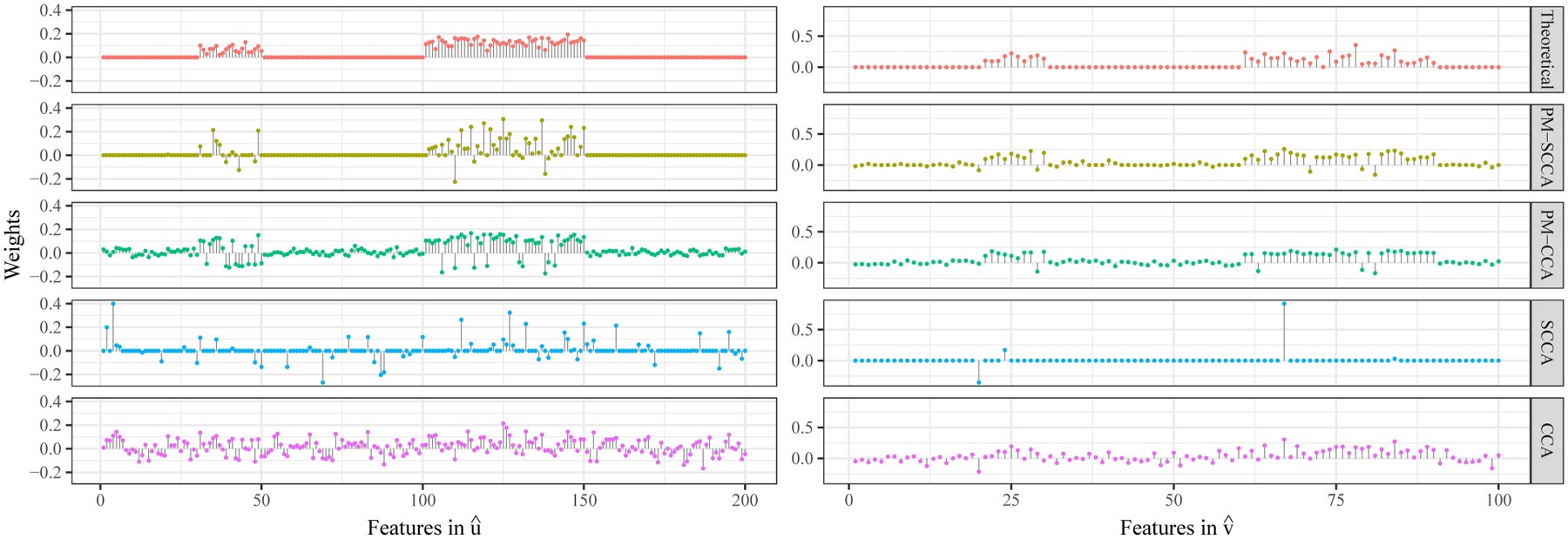
Estimated canonical weights of X features ($\widehat{u}$, left) and Y features ($\widehat{v}$, right) by PM-SCCA, PM-CCA, SCCA, and CCA on simulated data.⁺

2). Simulation results:

With n₀ = 2500 observations in total, we use n = 2000 for training-validation and n_t = 500 for testing for the simulation study. For each model, we first use 5-fold cross-validation for maximal validation canonical covariance to select optimal hyperparameters c₁, c₂, λ on the validation dataset and, with the selected hyperparameters, retrain the models on the training-validation subset to obtain $\widehat{u}$, $\widehat{v}$, the estimated canonical weights of the features in X and Y. Then, we calculate the canonical correlation (the expression in Eq (1)) both on the test subset and on the full dataset. The two most important goals that we wish to achieve with the proposed models are: (1) the features selected should be similar to the non-trivial features in the theoretical canonical weight vectors, and (2) the canonical correlation calculated with the estimated canonical weight vectors $\widehat{u}$, $\widehat{v}$ should be proximate to the theoretical canonical correlation.

Figure 1 shows the feature selection performance with $\widehat{u}$ and $\widehat{v}$ by PM-SCCA, PM-CCA, SCCA, CCA with their respective optimal sets of hyperparameters c₁, c₂, λ. Both PM guided methods correctly assigned large weights to the non-trivial features and small to zero weights to the trivial features in ground truth vectors u, v. In contrast, the features SCCA selected scarcely agree with either trivial or non-trivial features in the theoretical ground truth. The results by CCA contain excessive noises and therefore provide very limited information for interpretation in practice.

Table I lists the quantitative performance off our CCA models. We use canonical covariance for cross-validation because the simplified CCA models uses it as a part of the objective function for computation. On the other hand, since we are interested in how the results from the simplified models compare under the original settings of CCA models, we employ canonical correlation as the evaluation metric on both the test subset and the full dataset. As Table I shows, the testing canonical correlation by our proposed PM-guided methods is higher than their non-PM versions, respectively. This indicates that, our simplified PM-guided methods effectively yield generalizable results in the original CCA setting. Furthermore, it is evident that PM-SCCA successfully achieved the other important goal of recovering the canonical correlation recovered with $\widehat{u}$, $\widehat{v}$ evaluated on the full dataset as close to the theoretical canonical correlation as possible. One thing to note is that although the canonical correlation recovered by CCA is the highest one, it overestimated the theoretical canonical correlation and hence indicates that the model was overfitted with excessive trivial signals captured, which does not imply a superior performance.

TABLE I.

Model performance evaluation of PM-SCCA, PM-CCA, SCCA, and CCA on simulated data⁺

Method	CCov@Val*	CCor@Test	CCor@FullData#
PM-SCCA	11.12	0.1206	0.2867 (|D|=2.5)
SCCA	5.97	0.1022	0.2667 (|D|=22.5)
PM-CCA	7.46	0.1244	0.2447 (|D|=44.5)
CCA	2.81	0.0944	0.3819 (|D|=92.7)

^*The values are in the order of magnitude 1e-4.

^#The absolute difference is in the order of magnitude 1e-3 and calculated according to the theoretical canonical correlation on the actual synthetic data ρ₀=0.2892 instead of the target canonical correlation ρ=0.3.

^§CCov@Val denotes the canonical covariance on the validation dataset; CCor@Test denotes the canonical correlation on the test dataset; and CCor@FullData denotes the canonical correlation on the whole dataset.

B. Real data analysis

We apply the PM-SCCA algorithm to the SNP genetics data and multimodal QT data (i.e., gene expression, imaging and cognitive measures) from the Alzheimer’s disease neuroimaging initiative (ADNI) cohort. The goal is to identify interesting multi-SNP-multi-QT associations.

1). Data description and preprocessing:

The SNP and QT data used in preparation of this article were obtained from the Alzheimer’s Disease Neuroimaging Initiative (ADNI) database (http://adni.loni.usc.edu) [13]–[17]. The ADNI was launched in 2003 as a public-private partnership, led by Principal Investigator Michael W.Weiner, MD. The primary goal of ADNI has been to test whether serial magnetic resonance imaging (MRI), positron emission tomography (PET), other biological markers, and clinical and neuropsychological assessment can be combined to measure the progression of mild cognitive impairment (MCI) and early Alzheimer’s disease (AD). Up-to-date information about the ADNI is available at www.adni-info.org.

Following an Alzheimer’s Disease Modelling Challenge, named QT-PAD project (http://www.pi4cs.org/qt-pad-challenge), in this study, we included the following 16 QTs that have been shown to be significantly associated with AD:

• Five cognitive assessment scores measuring subjects’ memory and their ability of daily activities: ADAS13, CDRSB, RAVLT.learning, MMSE, and FAQ;

• Five whole-brain-level AD imaging and cerebrospinal fluid (CSF) biomarkers: FDG PET, Amyloid PET, CSF ABETA, CSF TAU, and CSF PTAU;

• Six FreeSurfer regional-level brain atrophy measurements [18]: FS WholeBrain, FS Hippocampus, FS Entorhinal, FS Ventricles, FS MidTemp, and FS Fusiform.

We removed all subjects with missing values on any of the 16 QTs. We selected the first visit of each subject in our study. All 16 QTs are normalized before being fed into the algorithm.

To test PM-SCCA, we also included 16 additional QTs that were not associated with AD. These were selected from the ADNI gene expression data. These data were generated using Affymetrix Human Genome U219 Array (Affymetrix, Santa Clara, CA) for expression profiling where the blood sample extraction, hybridization, and quality control process can be found in [13]. In the original data, one gene can correspond to multiple probes. We obtained the gene expression profiles by averaging all the probes for each gene across the subjects. We excluded all the AD-related genes indicated by NHGRI-EBI GWAS Catalog [19]. We randomly selected 16 gene expression profiles not associated with AD in the existing literature.

We downloaded genotyping data from ADNI 1, GO, 2, and 3 studies. We aligned and integrated the downloaded data using Homo sapiens (human) genome assembly NCBI37 (hg19) genome builder. We performed the strand alignment according to 1000 Genome phase 3 [20] using McCarthy Group Tools (https://www.well.ox.ac.uk/~wrayner/tools/). We imputed the genotyping data using the Michigan Imputation Server [21] with 1000 Genome phase 3 reference panel of European ancestry. We annotated our imputed genotyping data using ANNOVAR [22]. After alignment and imputation, we performed the quality control (QC) using the following criteria: genotyping call rate > 98%, minor allele frequency > 0.1%, Hardy-Weinberg Equilibrium > 1e-6, missingness per individual < 5%. We prioritized 12 SNP markers based on the major AD genome-wide association study (GWAS) findings [23]. We randomly selected 19 SNPs with no existing evidence indicating their significant associations with AD [19]. After QC and prioritization, our data were obtained by additive recoding the minor alleles per person. All the QC and recoding were performed using PLINK 1.9 [24]. After data preprocessing, we matched the common subjects in genotyping, gene expression, and QT-PAD challenge AD biomarkers. After matching, there are 343 subjects left with main characteristics summarized in Table II. We constructed our binary preference matrix by indicating the pairs of features that are significantly associated with AD in the corresponding dataset.

TABLE II. Participant characteristics.

Total number of subjects, age, and sex are shown in this table. The mean ± sd for the age of all subjects within each diagnosis group is reported. The number of male/female subjects within each diagnosis group is also introduced.

Diagnosis	CN	EMCI	LMCI	AD	Overall
Number	109	147	73	14	343
Age (mean ± sd)	74.55 ± 5.88	70.29 ± 7.40	72.51 ± 6.47	73.19 ± 11.60	72.23 ± 7.19
Sex (M/F)	56/53	77/70	44/29	8/6	185/158

2). Results and discussion:

Our real data analysis framework is shown in Fig. 2. We constructed two datasets. Each dataset consists of AD-related and AD-unrelated features. The preference matrix is constructed by indicating the pairs of features with significant AD relatedness. We applied our proposed PM-SCCA algorithm to identify multi-SNP-multi-QT associations in comparison with CCA, SCCA, and PM-CCA methods.

Fig. 2. Real Data Analysis.

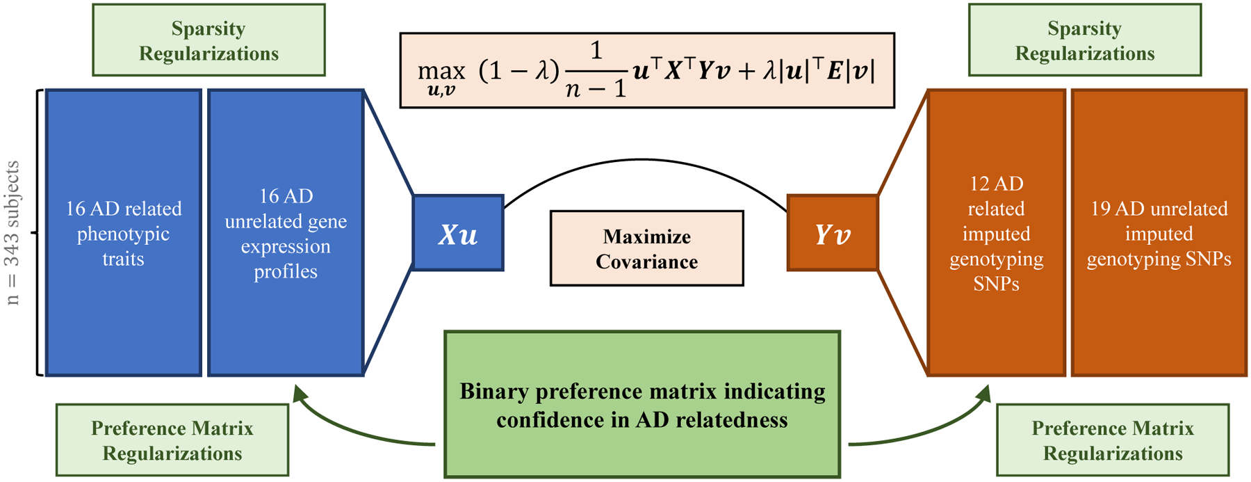
We constructed two datasets. Each dataset consists of AD-related features and AD-unrelated features. The preference matrix is constructed by indicating the pairs of features with significant AD relatedness.

We equally divided 343 subjects into 3 folds. Two folds were treated as a training-validation dataset and one fold was treated as a disjoint test set. To tune the hyperparameters c₁, c₂, and λ, we performed the three-fold cross-validation within the training-validation dataset. Four models were trained on two folds on the training-validation dataset and validated on the other one fold. Best-tuning hyperparameters were selected based on the highest average absolute validation canonical correlation. We re-trained our models with the best-tuned hyperparameter sets on the entire training-validation dataset and reported the canonical correlation as training performance. We applied the training model to the test dataset to obtain the testing canonical correlation.

Our results for real data analyses are reported in Table III. Overall, our proposed PM-SCCA model shows the highest testing canonical correlation. CCA, SCCA and PM-CCA methods show a large gap between training and testing canonical correlations, which indicates the potential overfitting issues. We plot the loading weight vector u and v of all four models for both datasets in Fig. 3. The CCA and SCCA models selected multiple AD-unrelated features. On the other hand, although the PM-CCA selected features are AD-related, the algorithm cannot achieve sparsity for revealing relevant genetic and phenotypic markers. Our PM-SCCA model assigned exact zero to those AD-unrelated features and identified AD-related features on both genotypic and phenotypic sides.

TABLE III.

Training and testing canonical correlations from real data analyses.

Methods	CCA	SCCA	PM-CCA	PM-SCCA
Training	0.371	0.367	0.237	0.264
Testing	−0.002	0.029	0.098	0.148

Fig. 3. Weight vectors $\widehat{u}$ and $\widehat{v}$ of all four models for imaging/cognition and genotyping datasets.

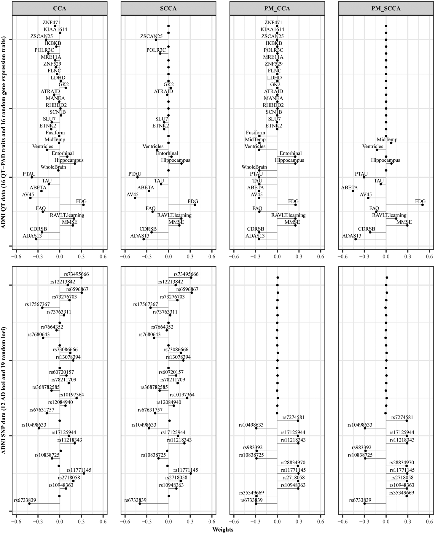
The top panel displays the feature selection results for the ADNI quantitative phenotype dataset. The top 16 features are AD-unrelated, whereas the bottom 16 features are AD-related. The bottom panel displays the feature selection results for the ADNI genotyping dataset. The top 19 SNPs are AD-unrelated, and the bottom 12 features are AD-related.

V. Conclusion

In summary, we have proposed a preference matrix guided sparse canonical correlation analysis (PM-SCCA) model to investigate the relationship between genetic variations such as SNPs and quantitative traits (e.g., molecular, imaging, fluid, cognitive QTs). Our model can detect biologically meaningful multi-SNP-mulit-QT associations and has the potential to provide new insights into AD. The incorporation of the preference matrix can facilitate the feature selection, where features proven to be related to AD are encouraged to be selected. Moreover, sparsity regularization can further achieve feature selections within the AD-related feature group. Our simulation study demonstrated that our models could both select the nontrivial features and recover the theoretical canonical correlation without overfitting. Our real data analysis demonstrated that our model could identify biologically interpretable features.

Our PM-SCCA study has potential limitations. First, due to the integrative analysis of multi-modal data, our study only includes a limited number of subjects. The small dataset may not have enough power to detect some weak signals and potentially leads to false negatives. Second, our PM-SCCA model can only leverage the information from one preference matrix at a time. In the future, the SCCA models that can simultaneously borrow information from multiple levels of prior knowledge are needed to mine biologically interpretable multi-SNP-multi-QT associations from multiple perspectives.

References

- [1].Shen L and Thompson PM, “Brain imaging genomics: Integrated analysis and machine learning,” Proceedings of the IEEE, vol. 108, no. 1, pp. 125–162, 2020. [DOI] [PMC free article] [PubMed] [Google Scholar]
- [2].Kim M, Min EJ, Liu K, Yan J, Saykin AJ, Moore JH, Long Q, and Shen L,“Multi-task learning based structured sparse canonical correlation analysis for brain imaging genetics,” Med Image Anal, vol. 76, p. 102297, 2022. [DOI] [PMC free article] [PubMed] [Google Scholar]
- [3].Du L, Huang H, Yan J, Kim S, Risacher SL, Inlow M, Moore JH, Saykin AJ, Shen L, and Alzheimer’s Disease Neuroimaging I., “Structured sparse canonical correlation analysis for brain imaging genetics: an improved graphnet method,” Bioinformatics, vol. 32, no. 10, pp. 1544–51, 2016. [DOI] [PMC free article] [PubMed] [Google Scholar]
- [4].Yan J, Du L, Kim S, Risacher SL, Huang H, Moore JH, Saykin AJ, Shen L, and Alzheimer’s Disease Neuroimaging I., “Transcriptome-guided amyloid imaging genetic analysis via a novel structured sparse learning algorithm,” Bioinformatics, vol. 30, no. 17, pp. i564–71, 2014. [DOI] [PMC free article] [PubMed] [Google Scholar]
- [5].Du L, Jingwen Y, Kim S, Risacher SL, Huang H, Inlow M, Moore JH, Saykin AJ, Shen L, and Alzheimer’s Disease Neuroimaging I., “A novel structure-aware sparse learning algorithm for brain imaging genetics,” Med Image Comput Comput Assist Interv, vol. 17, no. Pt 3, pp. 329–36, 2014. [DOI] [PMC free article] [PubMed] [Google Scholar]
- [6].Hardoon DR and Shawe-Taylor J, “Sparse canonical correlation analysis,” Machine Learning, vol. 83, no. 3, pp. 331–353, Nov. 2010. [Online]. Available: 10.1007/s10994-010-5222-7 [DOI] [Google Scholar]
- [7].Sun L, Ji S, and Ye J, “Canonical correlation analysis for multilabel classification: A least-squares formulation, extensions, and analysis,” IEEE Transactions on Pattern Analysis and Machine Intelligence, vol.33, no. 1, pp. 194–200, 2011. [DOI] [PubMed] [Google Scholar]
- [8].Witten DM, Tibshirani R, and Hastie T, “A penalized matrix decomposition, with applications to sparse principal components and canonical correlation analysis,” Biostatistics, vol. 10, no. 3, pp. 515–534, Apr. 2009. [Online]. Available: 10.1093/biostatistics/kxp008 [DOI] [PMC free article] [PubMed] [Google Scholar]
- [9].Witten DM and Tibshirani RJ, “Extensions of sparse canonical correlation analysis with applications to genomic data,” Statistical Applications in Genetics and Molecular Biology, vol. 8, no. 1, pp. 1–27, Jan. 2009. [Online]. Available: 10.2202/1544-6115.1470 [DOI] [PMC free article] [PubMed] [Google Scholar]
- [10].Parkhomenko E, Tritchler D, and Beyene J, “Sparsecanonical correlation analysis with application to genomic data integration,” Statistical Applications in Genetics and Molecular Biology, vol. 8, no. 1, pp. 1–34, Jan. 2009. [Online]. Available: 10.2202/1544-6115.1406 [DOI] [PubMed] [Google Scholar]
- [11].Liu K, Long Q, and Shen L, “Grouping effects of sparse cca models in variable selection,” arXiv preprint arXiv:2008.03392, 2020. [Google Scholar]
- [12].Min EJ, Chi EC, and Zhou H, “Tensor canonical correlation analysis,” Stat, vol. 8, no. 1, p. e253, 2019, e253 sta4.253. [Online]. Available: https://onlinelibrary.wiley.com/doi/abs/10.1002/sta4.253 [DOI] [PMC free article] [PubMed] [Google Scholar]
- [13].Saykin AJ, Shen L, Yao X, Kim S, Nho K, Risacher SL, Ramanan VK, Foroud TM, Faber KM, Sarwar N, Munsie LM, Hu X, Soares HD, Potkin SG, Thompson PM, Kauwe JS, Kaddurah-Daouk R, Green RC, Toga AW, Weiner MW, and Alzheimer’s Disease Neuroimaging I., “Genetic studies of quantitative mci and ad phenotypes in adni: Progress, opportunities, and plans,” Alzheimers Dement, vol. 11, no. 7, pp. 792–814, 2015. [DOI] [PMC free article] [PubMed] [Google Scholar]
- [14].Shen L, Thompson PM, Potkin SG, Bertram L, Farrer LA, Foroud TM, Green RC, Hu X, Huentelman MJ, Kim S, Kauwe JS, Li Q, Liu E, Macciardi F, Moore JH, Munsie L, Nho K, Ramanan VK, Risacher SL, Stone DJ, Swaminathan S, Toga AW, Weiner MW, Saykin AJ, and Alzheimer’s Disease Neuroimaging I., “Genetic analysis of quantitative phenotypes in ad and mci: imaging, cognition and biomarkers,” Brain Imaging Behav, vol. 8, no. 2, pp. 183–207, 2014. [DOI] [PMC free article] [PubMed] [Google Scholar]
- [15].Shen L, Kim S, Risacher SL, Nho K, Swaminathan S, West JD, Foroud T, Pankratz N, Moore JH, Sloan CD, Huentelman MJ, Craig DW, Dechairo BM, Potkin SG, Jack J, R. C, Weiner MW, Saykin AJ, and I. Alzheimer’s Disease Neuroimaging, “Whole genome association study of brain-wide imaging phenotypes for identifying quantitative trait loci in mci and ad: A study of the adni cohort,” Neuroimage, vol. 53, no. 3, pp. 1051–63, 2010. [DOI] [PMC free article] [PubMed] [Google Scholar]
- [16].Weiner MW, Veitch DP, Aisen PS, Beckett LA, Cairns NJ, Green RC, Harvey D, Jack CR, Jagust W, Liu E, Morris JC, Petersen RC, Saykin AJ, Schmidt ME, Shaw L, Shen L, Siuciak JA, Soares H, Toga AW, Trojanowski JQ, and Alzheimer’s Disease Neuroimaging I., “The alzheimer’s disease neuroimaging initiative: a review of papers published since its inception,” Alzheimers Dement, vol. 9, no. 5, pp. e111–94, 2013. [DOI] [PMC free article] [PubMed] [Google Scholar]
- [17].Weiner MW, Veitch DP, Aisen PS, Beckett LA, Cairns NJ, Green RC, Harvey D, Jack J, R. C, Jagust W, Morris JC, Petersen RC, Saykin AJ, Shaw LM, Toga AW, Trojanowski JQ, and I. Alzheimer’s Disease Neuroimaging, “Recent publications from the alzheimer’s disease neuroimaging initiative: Reviewing progress toward improved ad clinical trials,” Alzheimers Dement, vol. 13, no. 4, pp. e1–e85, 2017. [DOI] [PMC free article] [PubMed] [Google Scholar]
- [18].Fischl B, “Freesurfer,” NeuroImage, vol. 62, no. 2, pp. 774–781, 2012, 20 YEARS OF fMRI. [DOI] [PMC free article] [PubMed] [Google Scholar]
- [19].Buniello A et al. , “The nhgri-ebi gwas catalog of published genome-wide association studies, targeted arrays and summary statistics 2019,” Nucleic acids research, vol. 47, no. D1, pp. D1005–D1012, 2019. [DOI] [PMC free article] [PubMed] [Google Scholar]
- [20].1000 Genomes Project Consortium et al. , “A global reference for human genetic variation,” Nature, vol. 526, no. 7571, p. 68, 2015. [DOI] [PMC free article] [PubMed] [Google Scholar]
- [21].Das S, Forer L, Schonherr S, Sidore C, Locke AE, Kwong A, Vrieze SI, Chew EY, Levy S, McGue M, Schlessinger D et al. , “Next-generation genotype imputation service and methods,” Nat Genet, vol. 48, no. 10, pp. 1284–1287, 2016. [DOI] [PMC free article] [PubMed] [Google Scholar]
- [22].Wang K, Li M, and Hakonarson H, “Annovar: functional annotation of genetic variants from high-throughput sequencing data,” Nucleic acids research, vol. 38, no. 16, pp. e164–e164, 2010. [DOI] [PMC free article] [PubMed] [Google Scholar]
- [23].Lambert JC, Ibrahim-Verbaas CA, Harold D, Naj AC, Sims R et al. , “Meta-analysis of 74,046 individuals identifies 11 new susceptibility loci for Alzheimer’s disease,” Nature Genetics, vol. 45, no. 12, pp. 1452–1458, dec 2013. [Online]. Available: https://pubmed.ncbi.nlm.nih.gov/24162737/ [DOI] [PMC free article] [PubMed] [Google Scholar]
- [24].Chang C et al. , “Second-generation plink: rising to the challenge of larger and richer datasets,” GigaScience, vol. 4, 2015. [DOI] [PMC free article] [PubMed] [Google Scholar]