Modelling hydrological factors from DEM using GIS

Abstract

Hydrological modelling is a precondition for many scientific researches such as species distribution models, ecological models, agricultural suitability models, climatological models, hydrological models, flood and flash flood models, landslide models etc. Even the topographic control over many hydrological factors has also been studied. Over time different hydrological models have been developed and extensively used. Recently, these models have been used to prepare different types of conditional factors that are widely used in hazard modelling such as floods, flash floods, landslides etc. Quantitative analysis of the Digital Elevation Model (DEM) according to different models by engaging Geographic Information Systems (GIS) supports users to extract various types of information about landscapes where hydrological and topographic information are most important. Methods to prepare hydrological factors namely TWI, TRI, SPI, STI, TPI, stream density and distance to stream by processing DEM in GIS are discussed in this paper. These common hydrological factors are extensively used in many scientific research papers either for modelling or to measure their relationship with other environmental factors.

• •Hydrological factors have great importance in understanding the landscape and are widely used in scientific research, especially geo-environmental hazard mapping.
• •Physically based hydrological methods are engaged in ArcMap 10.5 software.
• •Commonly used hydrological factors are processed using freely available DEM and ArcMap 10.5 software.

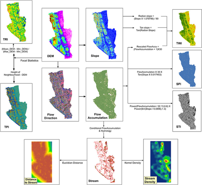
Graphical abstract

Specifications table

Subject area:	Environmental Science
More specific subject area:	Geology and hydrology
Name of your method:	Hydrological modelling for causative factor extraction
Name and reference of original method:	P.F. Quinn, K.J. Beven, R. Lamb, The in (a/tan/β) index: How to calculate it and how to use it within the topmodel framework, Hydrol pro. 9:2 (1995)161–182.10.1002/hyp.3360090204 K.J. Beven, M.J. Kirkby, A physically based, variable contributing area model of basin hydrology, Hydrol Sci J. 24:1 (1979) 43–69.10.1080/02,626,667,909,491,834 S.J. Riley, S.D. DeGloria, R. Elliot, Index that quantifies topographic heterogeneity, Int. J. Sci. 5:1–4 (1999) 23–27.
	I. Ahmad, M.A. Dar, A.H. Teka, T. Gebre, E. Gadissa, A.T. Tolosa, Application of hydrological indices for erosion hazard mapping using Spatial Analyst tool, Environ Monit Assess. 191 (2019) 482.10.1007/s10661-019-7614-x I.D. Moore, J.P. Wilson, Length-slope factors for the Revised Universal Soil Loss Equation: Simplified method of estimation, J. Soils Water Conserv. 47:5 (1992) 423–428. A. Weiss, Topographic position and landforms analysis. In Poster presentation, ESRI user conference, San Diego, CA. 200 (2001). A. Guisan, S. B. Weiss, A. D. Weiss GLM versus CCA spatial modelling of plant species distribution. Plant Ecol. 143 (1999) 107–122.10.1023/A:1,009,841,519,580 D. Djokic, Z. Ye, C. Dartiguenave, Arc hydro tools overview. ESRI. 5 (2011).
Resource availability:	Equipment: Digital Elevation Model (DEM) and Spatial Analysis toolset Data: Open Source DEM are available at USGS earth explorer (https://earthexplorer.usgs.gov/) Processed Data will be made available on request. Software: AcrMap 10.5 Hardware: CPU Speed 2.2 GHz minimum; Hyper-threading (HHT) or Multi-core recommended; Memory/RAM minimum 4 GB, recommended 8 GB; Disk space minimum: 4 GB recommended: 6 GB or higher; Display properties 24-bit colour depth

Introduction

Hydrological model and land surface characterization can predict both geomorphic processes and runoff characteristics (such as rate and patterns of runoff generation) over earth surface as well as over a large river basin. Spatial distribution of local slope and the drainage per unit contour length are the base of such physically based hydrological models. Digital elevation models (DEM) are most commonly used for land surface characterization and it supports to analyse the topographic attributes even for a large drainage basin by using hydrological model [1,2].

In recent years, the increased availability of DEM and the advances in geographic information systems (GIS) have supported a detailed and more realistic representation of surface topography [3]. As a result, hydrological modelling has become more accurate, detailed and less time-consuming [[4], [5]–6]. Several factors and land surface characteristics derived from hydrological model are popularly used in many scientific, engineering, and planning applications [2].

DEM-processed hydrological and topographical parameters have significant applications in species distribution modelling, climate modelling, agricultural suitability analysis, tree species modelling, hydrological modelling, landslide and flood assessment etc. Researchers across the world measured a good agreement of landslides and DEM processed topographical, morphological and hydrological factors [[7], [8]–9] such as slope aspect, slope angle, elevation, plan curvature, profile curvature, general curvature, topographic wetness index (TWI), stream power index (SPI), sediment transport index (STI), topographic roughness index (TRI), topographic position index (TPI), distance to stream density etc. In landslide susceptibility mapping and assessment, these factors are used as independent variables whereas landslides are used as dependant variables [10,11]. The practice of the use of these factors has increased due to the availability of open-source DEM data of the globe. The factors can be processed from DEM using GIS (ArcMap) software. (ArcMap) GIS is a very sophisticated software that allows processing raster data and storing the data of each cell of the raster. Besides, many in-built tools, the raster calculator also allows various types of complicated analysis that is very helpful in employing physically based hydrological models. In this part, hydrological modelling using Arcmap software is discussed which is very helpful, especially in hazard modelling.

Topographic wetness index (TWI)

The hydrological condition of an area is largely controlled by the topography of that area. Topography simply refers the undulation or unevenness of the surface. This unevenness (topography) is the first-order control on the spatial variation of hydrological properties of an area [12]. Beven and Kirkby (1979) [13] first introduced the concept of Topographic Wetness Index (TWI). Beven and Kirkby (1979) [13] proposed a hydrological forecasting model by which runoff generation over the surface of a basin is measured based on the water storage capacity and surface saturation of the soil of the basin area. The water storage capacity of soil was derived from the topographic condition of basin unit [13].

Nowadays Topographic Wetness Index (TWI) has been measuring from DEM (digital elevation model) [14] according to the grid unit of the DEM.

TWI is measured using the original topographic Wetness Index (TWI) proposed by Beven and Kirkby (1979) Eq. (1) [13]:

$$\mathit{TWI}=\ln \left(\frac{\alpha }{tan\beta }\right)$$ (1)

Where, α is the upslope contributing area per unit contour length, β is the slope angle/gradient and combined tan(β) represents the frequency distributions of slope/ steepest downslope direction.

Beven and Kirkby (1979) [13] proposed the model to calculate the local storage capacity of basin considering steady state conditions [11]. In a steady-state condition, accumulation of water trends at a given point. Where the local slope tan(β), described in Eq. (1), represents the effect of gravitational forces on water movement at that point [13,15].

In ArcMap software it is calculated using the following steps:

$$\begin{array}{c}\text{Radian}\text{slope}=\left(\text{“}\text{Slope}\text{ti}\mathrm{f}\text{''}*1.570796\right)/90\hfill \\ Tanslope=Con(\text{“}Radian\_slope.tif\text{''}>0,Tan\left(\left(\text{“}Radian\_slope.tif\text{''}\right),0.001\right)\hfill \end{array}$$

This condition is used to put a 0.001 value to the Radian Slope value less than 0. If the zero value is used in calculating Tan of slope, the value will be undefined that cannot be calculated and stored in the raster file. This value will not also be meaningful for further analysis.

To calculate TWI in Eq. (1), Ln will be used. But the “flow accumulation” raster has some 0 values that will be undefined in the calculation process and will produce errors. To remove this error (remove zero value), “flow accumulation” raster need to be rescaled by adding 1. The flow path will be calculated using the flow accumulation and multiplying the pixel size. The following command is used for this purpose:

$$\text{Rescaled}\text{flow}\text{accumulation}=(\text{“}\text{FlowAccu}.\text{tif}\text{''}+1)*30$$

Now the final TWI is calculated by dividing Rescaled flow accumulation by Tan slope Fig. 1.

Fig. 1.

TWI calculation.

Topographic Wetness Index (TWI) derived from digital elevation model is therefore often used as a proxy for soil moisture [14]. Flood-prone areas can be detected using TWI model [15]. Besides, TWI is also applied to assess topographic control on hydrological process [16], vegetation seasonality and aridity [17], plant species distribution, species assemblages and community diversity in riparian ecosystems [18]. TWI is found very efficient in ecosystem modelling [18]. This factor has been widely used in landslide susceptibility assessment and mapping.

TWI and soil depth has a positive correlation to subsurface saturation but varies spatially and temporally. There is a positive correlation between TWI and pore water pressure and this correlation increases and becomes more significant after the generation of new saturation [19]. The surface saturation increases the pore water pressure. Landscape soil moisture can be predicted from TWI and researchers reported various types of positive correlations comparing field observations and predicted TWI from different areas across the world [3]. Discrepancies of correlation between TWI and landscape-scale soil moisture aroused because of the differences in physiography, geology, climate, and vegetation pattern of the study area [3].

DEM resolution and calculation procedure of digital terrain analysis (DTA) have significant effects on statistical distribution and spatial pattern of the TWI indices [20,21].

Topographic roughness index (TRI)

Topographic roughness is synonymous to terrain complexity, surface roughness and rugosity. It describes the deviation of direction from the ideal or planned form of a normal vector of a defined surface [22]. So, roughness of terrain simply indicates the unevenness of elevation of centre cell from its neighbouring cells.

Riley et al. (1999) [23] provide the methodology of terrain roughness calculation which is commonly used for landslide spatial data preparation. According to Riley et al. (1999) [23], TRI can be calculated using Eq. (2). The value of a central cell (elevation of that cell) is subtracted from the neighbouring cell values (elevation). The resultant differences are multiplied by themselves, summed up and squared once again [24]. Elevation difference is first summed up and then multiplied or squared. The multiplied or squared value is squared again to get the final result TRI [25]. The equation is developed according to Fig. (2).

$$\mathit{TRI}=1/\cos \left(\tan \beta *\pi /180\right)$$ (2)

Fig. 2.

Neighborhood operations of a 3  ×  3 input cell block (Source: Habib 2021).

In ArcGIS, “focal statistics” tool is used to calculate the statistics of a focal cell within a defined moving window. This tool “calculates for each input cell location a statistic of the values within a specified neighbourhood around it”. Maximum, minimum and mean value of a cell from its neighbouring cell is needed to calculate for this purpose. The values can be directly calculated by specifying the required parameter in the “focal statistics” window. The following command is then used to calculate TRI values of each cell:

$$\left(\text{“}\text{Mean}\_\text{DEM}.\text{ti}\mathrm{f}\text{''}-\text{“}\text{Min}\_\text{DEM}.\text{ti}\mathrm{f}\text{''}\right)/\left(\text{“}\text{Max}\_\text{DEM}.\text{ti}\mathrm{f}\text{''}-\text{“}\text{Min}\_\text{DEM}.\text{ti}\mathrm{f}\text{''}\right)$$

Complexity arises because different window sizes will produce different results. It needs to be careful to define same window size for calculating a specific TRI, if put 10 × 10 window that should be followed every time. Fig. 3 shows the TRI calculation using 10 × 10 window.

Fig. 3.

TRI calculation.

Stream power index (SPI)

SPI indicates the power of erosive process caused by surface runoff [26,27]. It is measured using catchment area and slope of a defined area Eq. (3) [27]:

$$\mathit{SPI}=\left[\text{ln}\left({\mathrm{A}}_{\mathrm{s}}+0.001\right)\times \left(\left(\frac{\beta }{100}\right)+0.001\right)\right]$$ (3)

where As is the basin flow accumulation, β is the basin slope.

SPI helps in demarcating areas having potential to be saturated with water depending upon its contributing neighbourhood and the local slope gradient [28].

SPI is a secondary topographic attribute derived from the contributing area of flow accumulation and slope. The SPI determines the erosive power of the channel and expresses the topographic potential for deposition (for low or negative values) and erosive areas (positive values). The SPI for the study area was calculated using the following command line in the Raster Calculator [28]. Fig. 4 shows the SPI calculation process in ArcMap 10.5 software.

$$\text{“FlowAcc.tif}\text{''.*.30}·\text{*}\text{-}\text{Tan}(\text{“Slope.tif}\text{''}.*.0.017453)$$

Fig. 4.

SPI calculation.

Sediment transportation index (STI)

STI provides information on sediment transport capacity and accumulation and their spatial distribution [28]. There are various types of relationships found to measure STI, but the model proposed by Moore and Wilson (1992) [29] is the best suited to integrate into GIS platform [30]. According to Moore and Wilson (1992) [29], STI is a dimensionless index, a non-linear function between of specific discharge and slope. The index is a product of transport capacity limiting sediment flux in Hairsine-Rose, WPP, and catchment evolution erosion theories [29]. Moore and Wilson (1992) [29] proved that for a two-dimensional hillslope, the combined length-slope (LS) factor in the USLE (Universal Soil Loss Equation) and RUSLE (Revised Universal Soil Loss Equation) model is the measure of the sediment transport capacity of overland flow [29]. This sediment transport capacity is alternatively known as sediment transportation index. STI is calculated using the following formula Eq. (4) [28]:

$$\mathit{STI}=\left(m+1\right)\times \left(A_s/22.13\right)m\times \sin \left(\beta /0.0896\right)n$$ (4)

where “As” is the flow accumulation, “b” is the slope, “ln” is the Napierian logarithm, m = 0.4, and n = 1.3

The equation is proposed by Moore and Wilson (1992) [29], where, m is the area exponent and n slope exponent. The standard value of m is considered 0.6 which can vary from 0.4 to 0.6 and the standard value of n is 1.3 which can vary from 1.2 to 1.3. These two values, m and n, are used to “map the effects of hydrology, and hence 3-D terrain, on soil erosion in natural landscapes”. The As represents the effect of converging and diverging terrain on soil erosion which is the flow accumulation in ArcGIS software. β is the basin slope. The following command line in “raster calculator” is used to calculate STI in ArcMap software and Fig. 5 shows the calculation process of STI:

$$\text{Power}(\text{“FlowAcc.tif}\text{''}/22.13,0.6)*\text{Power}\left(\text{Sin}\right(\text{“Slope}\text{tif}\text{''}/0.0896),1.3)$$

Fig. 5.

STI calculation.

Sometimes, null value generates during analysis in ArcMap which creates problems in further analysis of the raster. To remove null values the following conditional analysis can be used:

$$\text{Con}\left(\text{IsNull}\left(\text{“}\text{STI}.\text{ti}\mathrm{f}\text{''}\right),0,\text{“}\text{STI}.\text{ti}\mathrm{f}\text{''}\right)$$

This will replace the null value to 0 values. In this map, this method is applied to remove null values.

Topographic position index (TPI)

The Topographic Position Index (TPI) compares the elevation of each cell in a DEM to the average height of the area around that cell Fig. 6. Although continuous circles or other shapes could be employed, in this example an annulus neighbourhood is chosen. Since a digital elevation model is the only input needed, TPI can be easily generated practically everywhere [31].

Fig. 6.

TPI and slope position (adopted from Weiss (2001)).

A positive TPI value indicates ridges that are above the neighbourhood average. A negative TPI value indicates valleys that are located below the neighbourhood locations. TPI value near 0 indicates the region has a constant slope (if the slope is significantly greater than 0) or the region is flat (slope is close to 0) [31,32].

Topographic position index largely depends on scale. Such as a region can be flat plain at 100 m scale. But if it is considered on a several-kilometre scale the same place can be a bottom of a canyon or deep valley. The TPI value of finer scale can be suitable for studying soil transport or site water balance. The coarser scale is more suitable for overall hydrology, mesoclimate, wind exposure, or cold air drainage study. Guisan et al. (1999) [33] measured a significant relationship between TPI and species distribution in Spring Mountains of southern Nevada [31].

The TPI algorithm can be analysed using Geographic Information Systems (GIS). The formula is used to compare the elevation of each cell with continuous circle surrounding that cell. The local neighbourhood of TPI is defined by window size in ArcMap software [32]. The local neighbourhood of each cell is measured using “Focal Statistics” tool of ArcMap software. According to ESRI (2022) [34], “the ‘Focal Statistics’ tool calculates for each input cell location a statistic of the values within a specified neighbourhood around it”. In this tool, user can define window size according to his choice and mean value can be extracted. This neighbourhood is then compared with the local elevation to extract the TPI values. The TPI calculation process is shown in Fig. 7. In ArcMap software it can be calculated using the following formula Eq. (5):

$$TPI=\text{zero}/\text{near}-\text{zero}-\text{flat}\text{or}\mathrm{a}\text{near}\text{continuous}\text{slope}$$ (5)

Fig. 7.

TPI calculation.

Stream extraction

Stream is extracted using Hydrology tool of ArcMap software. After “flow accumulation” and “flow direction” is calculated, “flow accumulation” value is conditionally divided to extract the higher-order streams. If whole value is given, all the probable streams will be produced. So, according to study area characteristics “flow accumulation” value should be conditionally deducted.

After that “Stream Order” tool of Hydrology toolset will be used to extract the streams according to Strahler's Stream Order. In ArcMap, Strahler's and Shrive's Stream order is found. This stream order is kept in raster format. Now it is needed to convert into shape file for further use. “Stream to Shape” tool is now employed to convert it into shape file format.

Distance to stream and stream density

Distance to stream can be measured using “Euclidian Distance” tool and Stream Density can be measured using “Density” tool of ArcMap software Fig. 8. The raster then can be classified using predefined classification system such as “natural break” or manually. Distance to stream and stream density has a significant application in landslide analysis. Besides, these factors are also widely used in morphometric characterization, micro-scale hydrological or climate modelling, species distribution and agricultural suitability analysis.

Fig. 8.

Stream extraction and stream density and distance to stream calculation.

Conclusion

In this paper, methods of hydrological modelling using open-source DEM and GIS are shown. A sample study area is shown for this analysis. Most of the methods are derived from run-off generation models but now these are significantly caught the attention of hazard modelling. Besides, basin-scale hydrological modelling and ecological modelling the factors have been significantly used in different types of hazard modelling, especially landslide, flood and flash flood analysis. We only showed the application of GIS in producing the factors and complexity that arise during analysis in GIS. Different resolutions of DEM will produce different results for the same study area. So the resolution of DEM should be defined according to the requirement of the research.

Different GIS software can also lead to great differences in the final result. Mixture of GIS software in between steps to prepare the final product also leads to significant differences [35]. Besides open-source DEM, DEM data of UAVs are also now becoming popular and this data has significant operational importance in scientific research. DEM produced from UAVs can also be analysed using this method.

CRediT authorship contribution statement

Md. Sharafat Chowdhury: Conceptualization, Methodology, Software, Visualization, Writing – original draft, Writing – review & editing.

Declaration of Competing Interest

The authors declare that they have no known competing financial interests or personal relationships that could have appeared to influence the work reported in this paper.

Data availability

• Data will be made available on request.

References

- 1.Moore I.D., Grayson R.B., Ladson A.R. Digital terrain modelling: a review of hydrological, geomorphological, and biological applications. Hydrol. Process. 1991;5:3–30. doi: 10.1002/hyp.3360050103. [DOI] [Google Scholar]
- 2.Zhang W., Montgomery D.R. Digital elevation model grid size, landscape representation, and hydrologic simulations. Water Resour. Res. 1994;30(4):1019–1028. doi: 10.1029/93WR03553. [DOI] [Google Scholar]
- 3.Buchanan B.P., Fleming M., Schneider R.L., Richards B.K., Archibald J., Qiu Z., Walter M.T. Evaluating topographic wetness indices across central New York agricultural landscapes. Hydrol. Earth Syst. Sci. 2014;18:3279–3299. doi: 10.5194/hess-18-3279-2014. 2014. [DOI] [Google Scholar]
- 4.Lacroix M.P., Martz L.W., Kite G.W., Garbrecht J. Using digital terrain analysis modeling techniques for the parameterization of a hydrologic model. Environ. Model. Softw. 2002;17(2):125–134. doi: 10.1016/S1364-8152(01)00042-1. [DOI] [Google Scholar]
- 5.Wang L., Liu H. An efficient method for identifying and filling surface depressions in digital elevation models for hydrologic analysis and modelling. Int. J. Geogr. Inf. Sci. 2006;20(2):193–213. doi: 10.1080/13658810500433453. [DOI] [Google Scholar]
- 6.Dongquan Z., Jining C., Haozheng W., Qingyuan T., Shangbing C., Zheng S. GIS-based urban rainfall-runoff modeling using an automatic catchment-discretization approach: a case study in Macau. Environ. Earth Sci. 2009;59(2):465–472. doi: 10.1007/s12665-009-0045-1. [DOI] [Google Scholar]
- 7.Budimir M.E.A., Atkinson P.M., Lewis H.G. A systematic review of landslide probability mapping using logistic regression. Landslides. 2015;12(3):419–436. [Google Scholar]
- 8.Süzen M.L., Kaya B.Ş. Evaluation of environmental parameters in logistic regression models for landslide susceptibility mapping. Int. J. Digital Earth. 2012;5(4):338–355. [Google Scholar]
- 9.Kanwal S., Atif S., Shafiq M. GIS based landslide susceptibility mapping of northern areas of Pakistan, a case study of Shigar and Shyok Basins. Geomat. Nat. Hazards Risk. 2017;8(2):348–366. [Google Scholar]
- 10.Hafsa B., Chowdhury M.S., Rahman M.N. Landslide susceptibility mapping of Rangamati District of Bangladesh using statistical and machine intelligence model. Arab. J. Geosci. 2022;15(15):1–21. doi: 10.1007/s12517-022-10607-3. [DOI] [Google Scholar]
- 11.Chowdhury M.S., Hafsa B. Landslide susceptibility mapping using bivariate statistical models and GIS in chattagram district, Bangladesh. Geotech. Geol. Eng. 2022;40:1–24. [Google Scholar]
- 12.Sørensen R., Zinko U., Seibert J. On the calculation of the topographic wetness index: evaluation of different methods based on field observations. Hydrol. Earth Syst. Sci. 2006;10:101–112. doi: 10.5194/hess-10-101-2006. [DOI] [Google Scholar]
- 13.Beven K.J., Kirkby M.J. A physically based, variable contributing area model of basin hydrology. Hydrol. Sci. J. 1979;24(1):43–69. doi: 10.1080/02626667909491834. [DOI] [Google Scholar]
- 14.Kopecký M., Macek M., Wild J. Topographic wetness Index calculation guidelines based on measured soil moisture and plant species composition. Sci. Total Environ. 2021;757 doi: 10.1016/j.scitotenv.2020.143785. [DOI] [PubMed] [Google Scholar]
- 15.Pourali S.H., Arrowsmith C., Chrisman N., Matkan A.A., Mitchell D. Topography wetness index application in flood-risk-based land use planning. Appl. Spatial Anal. 2016;9:39–54. doi: 10.1007/s12061-014-9130-2. [DOI] [Google Scholar]
- 16.Quesada-Román A., Ballesteros-Cánovas J.A., Granados-Bolaños S., Birkel C., Stoffel M. Improving regional flood risk assessment using flood frequency and dendrogeomorphic analyses in mountain catchments impacted by tropical cyclones. Geomorphology. 2022;396 doi: 10.1016/j.geomorph.2021.108000. [DOI] [Google Scholar]
- 17.Zhang X., Liu M. Topography regulates the responses of water partitioning to climate and vegetation seasonality. Sci. Total Environ. 2022 doi: 10.1016/j.scitotenv.2022.156028. [DOI] [PubMed] [Google Scholar]
- 18.Slezák M., Douda J., Šibíková M., Jarolímek I., Senko D., Hrivnák R. Topographic indices predict the diversity of Red List and non-native plant species in human-altered riparian ecosystems. Ecol. Indic. 2022;139 doi: 10.1016/j.ecolind.2022.108949. [DOI] [Google Scholar]
- 19.Liang W.L., Chan M.C. Spatial and temporal variations in the effects of soil depth and topographic wetness index of bedrock topography on subsurface saturation generation in a steep natural forested headwater catchment. J. Hydrol. 2017;546:405–418. [Google Scholar]
- 20.Zhang W., Montgomery D.R. Digital elevation model grid size, landscape representation, and hydrologic simulations. Water Resour. Res. 1994;30(4):1019–1028. doi: 10.1029/93WR03553. [DOI] [Google Scholar]
- 21.Quinn P.F., Beven K.J., Lamb R. The in (a/tan/β) index: how to calculate it and how to use it within the topmodel framework. Hydrol Pro. 1995;9(2):161–182. doi: 10.1002/hyp.3360090204. [DOI] [Google Scholar]
- 22.Whitehouse D.J. CRC Press; 1994. Handbook of Surface Metrology. [Google Scholar]
- 23.Riley S.J., DeGloria S.D., Elliot R. Index that quantifies topographic heterogeneity. Int. J. Sci. 1999;5(1–4):23–27. [Google Scholar]
- 24.Różycka M., Migoń P., Michniewicz A. Topographic Wetness Index and Terrain Ruggedness Index in geomorphic characterisation of landslide terrains, on examples from the Sudetes, SW Poland. Z. Fur Geomorphol. Supp Issues. 2017;61(2):61–80. doi: 10.1127/zfg_suppl/2016/0328. [DOI] [Google Scholar]
- 25.Habib M. Quantifying topographic ruggedness using principal component analysis. Adv. Civ. Eng. 2021 doi: 10.1155/2021/3311912. [DOI] [Google Scholar]
- 26.Jaafari A., Najafi A., Pourghasemi H.R., Rezaeian J., Sattarian A. GIS-based frequency ratio and index of entropy models for landslide susceptibility assessment in the Caspian forest, northern Iran. Int. J. Environ. Sci. Technol. 2014;11(4):909–926. doi: 10.1007/s13762-013-0464-0. [DOI] [Google Scholar]
- 27.Rahmati O., Kalantari Z., Samadi M., Uuemaa E., Moghaddam D.D., Nalivan O.A., Destouni G., Bui D.T. GIS-based site selection for check dams in watersheds: considering geomorphometric and topo-hydrological factors. Sustainability. 2019;11(20):5639. doi: 10.3390/su11205639. [DOI] [Google Scholar]
- 28.Ahmad I., Dar M.A., Teka A.H., Gebre T., Gadissa E., Tolosa A.T. Application of hydrological indices for erosion hazard mapping using Spatial Analyst tool. Environ. Monit. Assess. 2019;191:482. doi: 10.1007/s10661-019-7614-x. [DOI] [PubMed] [Google Scholar]
- 29.Moore I.D., Wilson J.P. Length-slope factors for the Revised Universal Soil Loss Equation: simplified method of estimation. J. Soils Water Conserv. 1992;47(5):423–428. [Google Scholar]
- 30.Bannari A., Ghadeer A., El-Battay A., Hameed N.A., Rouai M. Springer; Cham: 2017. Detection of Areas Associated With Flash Floods and Erosion Caused By Rainfall Storm Using Topographic attributes, Hydrologic indices, and GIS. In Global Changes and Natural Disaster management: Geo-information technologies; pp. 155–174. [DOI] [Google Scholar]
- 31.Weiss A. Topographic position and landforms analysis. Proceedings of the ESRI User Conference; San Diego, CA; 2001. [Google Scholar]
- 32.Masruroh H., Azmi S., Kristiawan I., Afdah U. Community survival strategy for environmental sustainability as adaptation in landslide threatened area: evidence from Malang, Indonesia. KnE Soc. Sci. 2022:1–10. doi: 10.18502/kss.v7i16.12147. [DOI] [Google Scholar]
- 33.Guisan A., Weiss S.B., Weiss A.D. GLM versus CCA spatial modeling of plant species distribution. Plant Ecol. 1999;143:107–122. doi: 10.1023/A:1009841519580. [DOI] [Google Scholar]
- 34.ESRI, How Focal Statistics works-ArcMap Documentation (2022). Available at: https://desktop.arcgis.com/en/arcmap/latest/tools/spatial-analyst-toolbox/how-focal-statistics-works.htm (Accessed: November 24, 2022).
- 35.Mattivi P., Franci F., Lambertini A., Bitelli G. TWI computation: a comparison of different open source GISs. Open geospatial data. Softw. Stand. 2019;4(6) doi: 10.1186/s40965-019-0066-y. [DOI] [Google Scholar]
Associated Data
This section collects any data citations, data availability statements, or supplementary materials included in this article.
Data Availability Statement