

Abstract
Purpose
Reliable process monitoring in real-time remains a challenge for the pharmaceutical industry. Dealing with random and gross errors in the process measurements in a systematic way is a potential solution. In this paper, we present a process model-based framework, which for given sensor network and measurement uncertainties will predict the most likely state of the process. Thus, real-time process decisions, whether for process control or exceptional events management, can be based on the most reliable estimate of the process state.
Methods
Reliable process monitoring is achieved by using data reconciliation (DR) and gross error detection (GED) to mitigate the effects of random measurement errors and non-random sensor malfunctions. Steady-state data reconciliation (SSDR) is the simplest forms of DR but offers the benefits of short computational times. We also compare and contrast the model-based DR approach (SSDR-M) to the purely data-driven approach (SSDR-D) based on the use of principal component constructions.
Results
We report the results of studies on a pilot plant-scale continuous direct compression-based tableting line at steady-state in two subsystems. If the process is linear or mildly nonlinear, SSDR-M and SSDR-D give comparable results for the variables estimation and GED. SSDR-M also complies with mass balances and estimate unmeasured variables.
Conclusions
SSDR successfully estimates the true state of the process in presence of gross errors, as long as steady state is maintained and the redundancy requirement is met. Gross errors are also detected while using SSDR-M or SSDR-D. Process monitoring is more reliable while using the SSDR framework.
Keywords: Data reconciliation, Direct compression, Monitoring
Introduction
Maintaining critical quality attributes (CQA’s) of the drug product within specified bounds is a significant concern in pharmaceutical manufacturing [1]. In traditional batch production, the CQA’s are typically monitored by statistical sampling of the finished dosage form and rejection of the batch if sampling indicates deviations from CQA specifications, leading to significant waste and increased cost [2]. Continuous manufacturing has been pursued by the industry and encouraged by regulators to overcome these limitations [3]. Effective continuous manufacturing is typically implemented using a real-time process management strategy, which encompasses multiple components. The first foundational component consists of real-time measurement and monitoring of the system including the use of process analytical technology (PAT) tools. The second involves a robust process control system. The third involves the detection, diagnosis, and mitigation of exceptional events. Finally, the fourth component requires real-time procedures for tracking and isolating non-compliant product [2]. This paper focuses on the first component.
Establishing an effective sensor network for monitoring CQA’s is a major step towards improving plant operations. However, measurements of CQA’s or related process variables can fluctuate over time due to random errors or to the occurrence of gross errors [4, 5]. Random errors cannot be predicted with certainty; they can only be characterized by probability distributions [6]. This type of the error can be caused by a variety of factors such as analytical errors or normal flow fluctuations, which cannot be entirely eliminated. By contrast, gross errors are caused by non-random events, such as a bias due to miscalibration, sensor degradation, or complete sensor malfunction [7]. Reliable process monitoring in real-time is still a challenge in continuous pharmaceutical manufacturing. Dealing with random and gross errors of the process measurements in a systematic way is a potential solution. The objective of this paper is to demonstrate a model-based framework, which for a given sensor network configuration and set of measurement uncertainties, will predict the most likely state of the process. Moreover, the capability of the methodology for the detection of gross errors in the process (GED) through statistical tests will be shown. Although data reconciliation (DR) has been widely used in other industries (i.e., oil and gas), to the author’s knowledge, it has not been applied to continuous pharmaceutical processes.
Alternatively, purely data-driven methods based on multivariate statistical models can also be used for state estimation [7, 8]. The model-based data reconciliation methods (SSDR-M) and the multivariate approaches generate comparable results under the assumption that the relationships between the measured variables are linear and certain additional assumptions hold true (Section “DR Using Multivariate Statistical Methods”) [9-11]. However, differences in reconciled values can occur if the process model involves nonlinear relationships between measured variables. SSDR-M also has the advantage that it can provide estimates of unmeasured variables through the model equations. In this paper, we report on the real-time application of both methodologies for DR and GED to a direct compression line, which involves the online use of load cells and near-infrared (NIR) spectroscopy-based sensors.
Theory
Data Reconciliation
The purpose of data reconciliation is to obtain the best estimate of the process measurements in the presence of random errors in the measurements [10]. Data reconciliation can be posed as an optimization problem in which the objective function (see Eq. 1), and the process model (Eqs. 2 and 3) are functions of the process variables. The process model usually consists of mechanistic relations (e.g., mass balances, energy balances), which are dependent on both measured and unmeasured variables as well as parameters. The key requirement is that the estimate of the process variables must satisfy the process model while optimizing a likelihood function. The mathematical formulation of an SSDR problem is given as below:
| (1) |
| (2) |
| (3) |
where is a vector of measurements, is a vector of reconciled values of the n measurements, is a vector of the m unmeasured process variables, Q is the covariance matrix, , is a vector of p process model parameters, is a set of equations which describe the steady-state behavior of the process, is a set of inequality constraints, n is the number of reconciled variables, m the number of unmeasured variables, and k the number of relations or equations.
The measured variables are assumed to be contaminated with random errors that are normally distributed with zero mean and known variances/covariances. Note that the objective function only contains terms corresponding to the measured variables. The unmeasured variables can be calculated from known variables and the process model, providing that the unmeasured variables are observable. Tests for observability are available in the literature [9, 12]. In general, DR requires that the process under study have positive degrees of freedom, that is, n + m − k > 0. Otherwise, there may be no feasible solution to Eq. 2. Therefore, there must be measurement redundancy in the process, requiring the deployment of sufficient PAT measurement points.
The process model used in DR can either describe the steady-state behavior of the process as shown in Eq. 2 or its dynamic behavior, in which case the process model will consist of a system of algebraic and differential equations. Dynamic models can represent the departures of the process variables from the steady-state and thus allow dynamic DR to be performed during transitions from steady-state, but the computational time for solving the dynamic DR problem will be much higher [13]. Other techniques for dealing with noisy measurements which do not require steady-state requirement include the family of Kalman filters. Although the classical Kalman filter (KF) does not have the steady-state requirement, it is applicable to linear and unconstrained systems. If the process is nonlinear and with hard constraints, modifications have been proposed, such as the extended Kalman filter (EKF) [14].
Moreover, dynamic data reconciliation approaches are also available and these do allow capturing of process dynamics [15]. Moving horizon estimation (MHE) is another technique used for treating noisy dynamic processes which is found to perform better than EKF usually [16]. However, the primary limitation of these approaches is the computational time required for their use in real time, especially for processes with fast dynamics.
The advantage of steady-state models is that they can be solved in computational time that allows the effective real-time use of the results; however, they are only valid during steady-state periods and, hence, require that the observed variations be around a steady state. Of course, steady state should be understood to mean that variations in process variables are within an allowable range determine via appropriate statistical tests. Consistent with the steady-state assumption, each measurement in the vector x is assumed to be made synchronously, that is, recorded at the same time point.
In general, steady-state process models (Eq. 2) consist of material balances, energy balances, design, and other empirical relationships as well as equations relating process variables to material physical and chemical properties. While component material balances are linear in the component flows, the energy balances are typically bilinear while the physical property, equipment, and performance are generally nonlinear. Consequently, although in the linear case, the solution of the DR problem can be expressed analytically and computed using projection matrix constructions [17], in the presence of nonlinear model elements, the DR problem must be solved numerically using nonlinear programming algorithms [10, 13]. In the continuous direct compression tableting line example discussed in subsequent sections of this paper, the SSDR model involves linear component material balances, energy balances are not required, and the only nonlinearities are introduced through property measurements, specifically those of stream composition.
The SSDR problem is typically solved using a two-step approach; first, for given values of the model parameters, the measured variables are reconciled. In the second step which usually is executed less frequently than the first step, the model parameters are (re-)estimated [18] using measurements from a sufficiently large number of sample points. The case studies reported in this paper only discuss the first step.
DR Using Multivariate Statistical Methods
Multivariate statistical process control (MSPC) methods involve the use of principal component analysis (PCA) or partial least squares (PLS) to monitor measured variables in a reduced space and detect process upsets through statistical tests [19]. PCA models represent the system through a subset of the principal components (PC’s) or latent variables by capturing most of the high-dimensional data (X) variance [20, 21]. PCA model can be expressed in scores (T) and loadings (P). The scores are the projections of each observation onto a subspace. The loadings are the eigenvectors associated with the eigen-values of the covariance matrix. There are additional forms of multivariate models, such as PLS, which represents X using a reduced number of latent variables (LV) while also representing the space of response matrix (Y) [22, 23]. In other words, PLS uses latent variables to capture the variation in X, and that is predicted in the Y [22, 24].
PCA is widely used for both monitoring and abnormal events detection. For the training of the PCA model, it is necessary first to obtain a sufficient number of instances of the measured variables, as training data. Then the loading matrix P is computed, as shown in Eqs. 4 and 5: the direct eigenvector-eigenvalue calculations or the nonlinear iterative partial least squares (NIPALS) algorithm can be used for this purpose.
| (4) |
| (5) |
where is the matrix of observed variables, is the principal components or scores matrix, is the loading matrix, is the random error matrix for X, n is the observed values, N is the number of observations, and d is the degrees of freedom or the number of PC’s where d < <n.
While PCA models are most commonly used for monitoring, it is less known [10] that such models can also be used to compute reconciled values of the measured variables Xm. As shown, Eq. 6 can be used to compute the updated scores from the new values of the measured variables and the loadings matrix. Then, the new estimated scores and loading matrix can be used to compute the reconciled values of the measured variables as shown in Eq. 7. These estimated values will be equivalent to the reconciled values obtained using the model-based approach, if certain conditions are met [10, 11, 25]. The scores and loadings can also be used in the statistical tests for GED (see Section “Error Detection”) for the reconciled values.
| (6) |
| (7) |
where is the matrix of the new measured variables, is the new principal components or scores matrix used for the new measured variables, is the matrix of the reconciled values for the measured variables through PCA, n is the observed values, N is the number of observations, and d is the degrees of freedom or the number of PC’s, where d < <n.
There are some key similarities and differences between the model and data-driven-based approaches for reconciliation and monitoring. In both cases, the covariance matrix must be obtained from historical data, that is from a training set of measured variable observations while the process is at steady-state(s). If it is assumed that an (n-k) set of principal components is used, the measurement errors are independent and identically distributed and the process model is linear, then the DR and PCA-based approaches are also comparable, and the latter method can be used for SSDR-D. Moreover, as shown in [10], the constraint matrix can also be estimated through PCA and will be equivalent to the DR model except for a rotational transformation of the data matrix. In [10], the authors further propose a framework for using DR and PCA in a complementary fashion and provide seven examples which employ simulated scenarios for a water distribution system.
There are differences that arise in how these approaches deal with gross errors and how the unmeasured variables are estimated. In SSDR-M, once the measurement with which the gross error is associated is identified, it is removed from the reconciliation process, the remaining measured variables are reconciled again, and the measurement with gross error is treated as an unmeasured variable. Since the process model already includes a mechanistic or empirical equation relating the measured variables to the unmeasured variable, the new set of reconciled values can be used to generate an estimate of the measurement that is in gross error.
In the SSDR-D case, the prediction of the measurement that is in gross error usually is treated as a missing variable. There are three approaches for handling missing variables in PCA that are used in industrial practice [26]: single component projection derived from the NIPALS algorithm, projection to the model plane, and conditional mean replacement, with the last one, generally regarded to be superior. By using this method, it is possible to replace the missing variable (i.e., measurement with gross error) by its conditional mean given by the other observed variables [26]. The conditional mean is estimated with the observed variables (with no gross error), using a standard score estimation routine. In common practice, the limit for application of these methods is to have no more than 20% of the variables missing, while in complex industrial problems it can go up to 30–60% [27]. Of course, PCA cannot estimate unmeasured variables when there is no training data.
The goal of this work is to demonstrate a systematic framework for dealing with measurement errors in order to estimate the “true” state of the process. We apply both approaches as applicable, establish their limitations, and demonstrate their performance in simple cases arising from the continuous tableting line via direct compression.
Error Detection
Model-Based Alternative
The DR methodology, whether process model-based or data-driven, generates reconciled process variable values, under the assumption that errors in the measured variables are random. If a non-random, so-called gross, error arises in a measurement, then that measurement will bias the reconciliation outcome. Thus, if such a gross error occurs then it must be identified, the faulty measurement discarded and the remaining measurements reconciled, as noted in the previous section. Detection of gross errors can readily be performed through the use of appropriate statistical tests, which are similar to outlier detection schemes employed in regression development.
There is a considerable literature on various tests for gross error detection (GED) proposed for use in DR. In this work, we employ two well-known tests: the global test and the measurement test. The global test (GT) serves to detect if there is an appreciable measurement error in the process [5, 6]. It can be shown that the maximum likelihood function (Eq. 1) evaluated at the reconciled values follows a chi-squared (χ21−α) distribution. The χ21−α is a function of the linearly independent equations (I) and the selected level of significance α (e.g., 5%). Thus, if the value of the objective function is greater than the chi-squared test criterion, then it is likely that a gross error has occurred.
However, the global test does not pinpoint which measurement is at fault. A second test, called the measurement test, can help to indicate where the gross error is located. It uses the magnitude of the variable corrections to identify those that are “large” relative to standard deviation and thus suspected. Improved results can also be obtained by using nonlinear programming (NLP) methods via the modified iterative measurement test (MIMT) algorithm [28]. The framework, shown in Fig. 1, summarizes the steps which are followed in the reconciliation process used in this study.
Fig. 1.
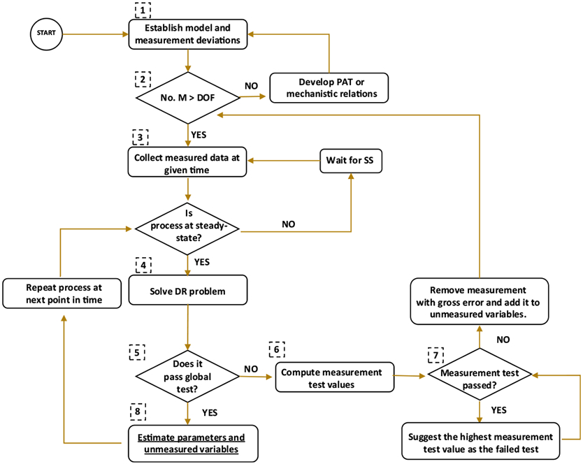
SSDR-M logic flow
The GED test can be applied to DR applications involving either linear or nonlinear process models. However, since the measurement test is defined in terms of the coefficient matrix of the linear model, in the nonlinear case, this requires some modification. Specifically, this matrix must be replaced by a linearization of the process model constructed at the nominal steady-state values of the process variables. Equation 8 represents the model constraints in linear form.
| (8) |
where is the linear constraint matrix, is a vector of reconciled values, and is a vector of known coefficients.
The details of measurement test are summarized in the following relationships:
| (9) |
| (10) |
| (11) |
| (12) |
where is a vector of measurements, is a vector of reconciled values, is a vector of errors, Q is the covariance matrix, , is the matrix of coefficients of the linear/linearized process model, is a vector of the measurement test values, VII is the index, n is the number of measurements, α is the level of significance (e.g., 5%), and β is the modified level of significance since it is a function of α and the number of measurements.
It can be shown that the difference vector (ai) follows a multivariate normal distribution with an expected value of zero and covariance given by Eqs. 9, 10, 11, and 12. Furthermore, the measurement test value mti follows a normal distribution with mean 0 and standard deviation of 1 [28]. Thus, if the mti is larger than the upper critical value (zα/2), most likely that measurement xi involves a gross error. Another type of critical value (z1−β/2) can also be considered which involves the number of measurements and the probability of error in each measurement. If there is a gross error and the measurement test cannot detect it, it is necessary to take the highest measurement test value and suggest it as a gross error. However, it is important to note that this decision is effectively a heuristic.
Finally, it should be acknowledged that process faults can arise from causes other than sensor failures. Such faults will give rise to significant departures of process variables outside of the range of variations that will be accepted by the steady-state test and, thus such, exceptional events will require active intervention in the process. In general, they will lead to the production of material outside of quality limits. The gross error detection methodology outlined above is based on the assumption that the process is at steady state, that such exceptional events have not occurred, and thus that the gross errors that arise lie with the measurements. There is an extensive literature on process fault detection and diagnosis which discusses these issues to which we direct the interested reader (see for example [29]).
Data-Driven Alternative
In the case of the SSDR-D approach, there is a two-criteria statistical test in common use to check if there are gross errors: The square prediction error (SPE) and the Hotelling’s T2. The SPE, (see Eq. 13), considers the model and measurement mismatch; it relates the orthogonal distance between the model plane and a given observation test [30]. The Hotelling’s T2, Eq. 14, describes the overall distance from the model and the observation [22, 31]. The confidence intervals for these tests can be found in the literature [26, 28].
| (13) |
| (14) |
where is a vector of measurements, is a vector of reconciled values, is the vector of scores for d degrees of freedom, and S the variance matrix for the scores generated in the training data, .
In order to identify the location of the gross error, it is necessary to check the difference between the reconciled and measured variables, that is the contribution of each variable to the SPE and the Hotelling’s T2 criteria. Equation 15 shows the power contributions (spei) of each variable [32]. Equation 16 represents the contributions done to the Hotelling’s T2.
| (15) |
| (16) |
SSDR Frameworks
In this section, we summarize the logic flow for the reconciliation and error detection procedures, which were discussed separately in the previous sections. Both the model-based and the data-driven frameworks incorporate repeated cycles of error detection to accommodate the situation in which multiple gross errors may arise.
SSDR-M Framework
The first two steps of the logic flow summarized below deal with defining the sensor network, process model and confirming observability of the unmeasured variables in the process model. The remaining steps 3–8 are repeatedly executed at each successive measurement time.
SSDR-M Logic
Step 1. Formulate the DR problem: Define the sensor network structure and determine the variance/covariance of the sensor measurements. Establish the steady-state process model equations and the set of measured and unmeasured variables. Test the unmeasured variables for observability.
Step 2. Redundancy check: Confirm that the number of measurements (No. M) is greater than the system degrees of freedom (DOF) and go to step 3. If the number of measurements is equal or less than the system degrees of freedom, DR cannot be performed, and additional sensors need to be added to the sensor network
Step 3. Test that the system is at steady-state and if so record all of the sensor measurements at a given time. It is possible to check for steady state by applying statistical tests. In the literature, there are different ways to detect steady state reported [33]. One approach is to perform a linear regression over a data window and a t test; if the slope is different from zero, then there is not steady state [34]. It is also possible to do an F test or R test to determine if the process is at steady state [35]. A simpler way to determine steady state is the use of statistical process control chart (SPC) moving average chart with a threshold of 3σ [25, 24]. If there is missing data (e.g., fouling, disconnection), treat the variable as an unmeasured variable.
Step 4. Solve the reconciliation problem to obtain reconciled values of measured variables.
Step 5. Execute the global test. Please note that the χ21−α is calculated based on the confidence interval and the number of independent equations. If the global test fails, proceed to step 6. If the global test is passed, go to step 8.
Step 6: Compute the measurement test value. If the process model is nonlinear, use the linearization at the steady-state operating point to estimate matrix A in Eq. 8.
Step 7. If one or more of the measurement test values is greater than the critical value (mti > zα/2), the measurement test failed. If the measurement test passed and the global tests did not, then select the measurement test that has the highest value and remove said measurement from the objective function. However, it should be noted that this decision criterion which is commonly used does constitute a heuristic. The measurement that was removed from the objective function will be considered an unmeasured variable; therefore, it has to be added to the said set. Go back to step 2.
Step 8. Compute the unmeasured variables using the reconciled measurement vector. If the model involves parameters, it may be necessary to re-estimate them using the reconciled values of the variables. Go to step 3 and repeat the process with at the next measurement time.
SSDR-D Framework
In the multivariate statistical method-based alternative, the process model is replaced by a PCA model that is constructed from historical data collected from the process at normal steady-state operating conditions (NOC). Once the PCA model is constructed and a subset of principal components selected, the process of computing reconciled measured, and corresponding estimates of unmeasured values are repeated with each new measurement set, followed by the application of selected statistical tests, such as the SPE, to detect gross errors. Figure 2 shows the SSDR-D framework flow.
Fig. 2.
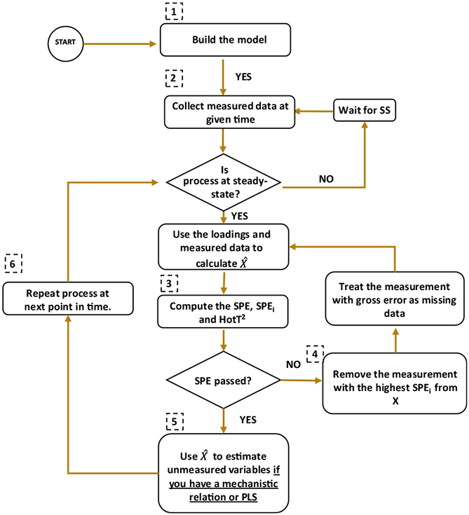
SSDR-D logic flow
SSDR-D Logic Flow
Step1. Model building: Determine the error covariance matrix and select historical data at NOC, without outliers. Train the PCA model and evaluate the number of principal components. Cross-validate the model and validate it with a new data set. If the system has unmeasured variables, add a PLS model or mechanistic relations to estimate them using .
Step 2. Check that the process remains at steady-state [34]. Given the measured data at a given point in time, use the model to monitor the process; it is necessary to reconstruct the observations by using the Tm and P loadings as in Eq. 7.
Step 3. Choose a confidence interval (i.e., 99%) and detect outliers in the process using Eq. 13, which represent the SPE statistical tests [36]. SPE follows a χ2 distribution, similar to the GT. If any of these tests values are larger than the confidence interval, most likely there is a gross error, go to step 4. If not, proceed to step 5.
Step 4. Evaluate the power contributions per variable and select the highest one; most likely, that is the measurement that has the gross error. Treat the measurement with gross error as missing data and go to step 1.
Step 5. Accept the reconstructed values from Eq. 7 and estimate the unmeasured variables through a PLS model or appropriate mechanistic relations established in step 1.
Step 6. Repeat algorithm at the next point in time.
Application Studies
Solid dosage tablets, the dominant dosage form for oral drug delivery, can be produced via continuous direct compression (DC). In this process, the active pharmaceutical ingredient (API) and the excipients are fed using loss-in-weight feeders, continuously blended and conveyed into the tablet press to produce the tablet [37]. The main CQA’s of tablets produced in a direct compression line are tablet composition, tablet hardness, tablet weight, and physical dimensions as well as tablet dissolution characteristics. In-process controls may include CPP’s and CQA’s such as mass flows of the feed materials and powder blend, blend composition, and tablet production rate.
Experimental System
For illustrative purposes, two cases will be presented that focus on the powder feeding and mixing components of the process. Figure 3 shows the block diagram of the continuous tableting pilot plant under study and highlights the subsystem we studied. Example 1 (E1) consists of two feeders: feeder 1 provides the API flow (FAPI) and feeder 2 the excipient flow (Fexc), followed by the blender. Example 2 (E2) consists of the E1 system followed a third feeder (Flube) and another blender. The main CQA’s and CPP’s in this subsystem are powder blend composition after each blender and the powder flows.
Fig. 3.
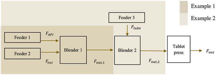
Block diagram of the direct compression tableting line. Feeder and blender subsystems
Materials and Equipment
Feeder 1 and feeder 2 are Schenck AccuRate AP-300 feeders, which transport acetaminophen (APAP obtained from Mallinckrodt Inc., Raleigh, North Carolina) and Avicel Microcrystalline Cellulose pH 102 (MCC 102, acquired from FMC BioPolymer Corporation in Philadelphia, Pennsylvania). Feeder 3 is a PUREFEED DP-4 Disc Feeder that introduces magnesium stearate (MgSt, from Spectrum Chemical Manufacturing Corporation in Gardena, CA) for example 2 case I and silicon dioxide (Cab-O-Sil untreated fumed silica, obtained from Cabot) for example 2 case II. The feeders use load cells to measure the weight-loss, have a scan rate of 16 million counts per minute and use a window time of 10 s to average said measurement. The feeder has an internal proprietary proportional-integral (PI) feedback controller, which based on changes in the weight-loss measurement, sends a signal of 4–20 mA, to the auger motor to increase or decrease the speed. The two blenders are Gericke GCM 250 mixers, which are operated at 200 rpm in the experiments reported herein.
PAT Tools and Sensor Calibration
In the case of E1, the APAP composition (xAPI,1) at the outlet of blender 1 is measured using a CDI-256-1.7T1 NIR spectrometer and the total flow with a Mettler Toledo balance. The Mettler Toledo balance arrangement is not a common PAT tool, but it is used for these experiments for convenience in demonstrating the SSDR framework. The CDI-NIR collects eight spectra of the flowing blend stream every second with an integration time of 4 ms, using wavelengths from 904 to 1687 nm [38]. The CDI spectra are related to APAP composition through a calibration function, which must be developed specifically for the materials processed. Calibration should ideally be done at production flow rate, although smaller flow rates are acceptable. The calibration was executed at a flow rate of 10 kg/h, and the Solvias Turbido NIR probe was positioned to be perpendicular to the powder flow. The combination of measurement and calibration function can be viewed as a chemometric model. The API composition measurement at the exit of the first blender (xAPI,1) employs a chemometric model that uses a PLS model (CDI-NIR sensor 1) with two principal components. The spectra pretreated using the Savitzy-Golay filter, first derivative and standard normal variate (SNV), over a 5–17% (wt.) APAP composition range and MCC200 as the excipient, following a method similar to that employed by Vanarase et al. [39]. For purposes of E2, the Mettler Toledo balance was moved to the exit of the second blender. The API composition measurement at the exit of the second blender (xAPI,2) employs a chemometric model that uses a PLS model (CDI-NIR sensor 2) with three principal components. The spectra pretreated using the Savitzy-Golay filter, first derivative, and SNV, over a 5–15% (wt.) APAP composition range, 0.2% silicon dioxide (SiO2), and the rest of the mixture was MCC200. Figure 4 shows the equipment and the sequence used in the pilot plant for each example.
Fig. 4.
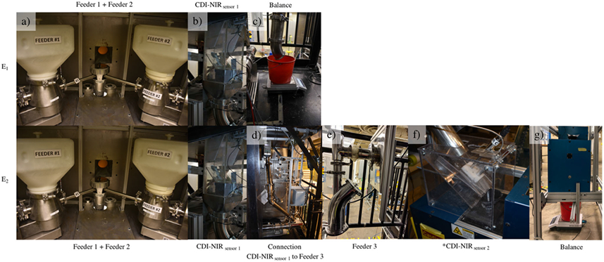
Feeder and blender PAT tools location according to E1 and E2. The API and excipient feeders load cells (a), CDI-NIR probe at the exit of the first blender (b), the Mettler Toledo balance (c), the connection between the first to the second blender (d), the lubricant feeder load-cell (e), CDI-NIR probe at the exit of the second blender (f), and the Mettler Toledo balance at the exit of the second blender (g). *Only applicable for E2, case 2
Estimation of Reconciled Values
SSDR Model (SSDR-M)
At steady state, the feeder and blender subsystem can be represented through simple material balance relations, consisting of Eqs. 17 and 18. It is assumed there is no material loss in the process. This assumption is only used for building the steady-state model. Material loss can be detected by data reconciliation. Of course, all flows have to be non-negative, and the composition in the range of 0 to 100 (%wt.).
| (17) |
| (18) |
where FAPI is the reconciled value of the API flow (kg/h), Fexc is the reconciled value of the excipient flow (kg/h), xAPI, 1 is the reconciled value for the API composition at the exit of the first blender (%wt), and Fout, 1 is the reconciled value of the outlet flow of the first blender (kg/h). In this simple example, there are four measured variables and two degrees of freedom.
In the E2 example, the lubricant flow and the composition at the exit of the second blender are additional variables. Equation 19 represents Eqs. 17 and 18 rearranged, while Eqs. 20, 21, and 22 represent the additional constraints. Note that in E1, all variables are measured; while in E2, Fout, 1 becomes an unmeasured variable. In addition, in E2, the composition measurements at the exit of the second blender are also unmeasured variables. Potentially, another NIR sensor could be added to monitor the composition of this stream. Table 1 lists the Q of the measurements, where Q is the known covariance matrix based on the measurements relative standard deviation. In the case of E2, there are five measured variables, three unmeasured variables and three degrees of freedom (see Table 1). Usually, Q for SSDR-M is determined from historical data. In these case studies to facilitate comparison, the Q used in SSDR-M (shown in Table 1) is computed from the SSDR-D training data.
| (19) |
| (20) |
| (21) |
| (22) |
where FAPI is the reconciled value of the API flow (kg/h), Fexc, 1 is the reconciled value of the excipient flow (kg/h), Flube is the reconciled value of the lubricant flow (kg/h), xAPI, 2 is the estimated value for the API composition at the exit of the second blender (%wt), xlube is the estimated value of the lubricant composition at the exit of the second blender (%wt), and Fout, 2 is the reconciled value of the outlet flow of the second blender (kg/h).
Table 1.
Normal operating conditions and covariance of the feeder blender subsystem
| Variable | Equipment | Set point |
Q (%) |
Type of variable |
||||
|---|---|---|---|---|---|---|---|---|
| E1 | E2, case I | E2, case II | E1 | E2, case I | E2, case II | |||
| FAPI (kg/h) | Load cells | 1 | 2 | 7 | 1 | Measured | Measured | Measured |
| Fexc (kg/h) | Load cells | 9 | 2 | 7 | 2 | Measured | Measured | Measured |
| xAPI,1a(% wt) | CDI-NIR | 10 | 6 | 6 | 4 | Measured | Measured | Measured |
| Fout,1a (kg/h) | Load cells | 10 | 8 | – | – | Measured | Unmeasured | Unmeasured |
| Flube (kg/h) | Load cells | 0.05 | – | 15 | 15 | NA | Measured | Measured |
| xAPI,2a (% wt) | CDI-NIR | 9.9 | – | – | 6 | NA | Unmeasured | Measured |
| xlubea (% wt) | CDI-NIR | 0.5 | – | – | – | NA | Unmeasured | Unmeasured |
| Fout,2a (kg/h) | Load cells | 10.05 | – | 8 | 8 | NA | Measured | Measured |
Average using a window time of 10 s. Q was determined using the training data for the multivariate model
For purposes of solving the maximum likelihood optimization problem, the feeder flows are bounded from 0 to 50 kg/h, the two API composition from 0 to 100%, the lubricant composition 0 to 2%, and the total flows from 0 to 100 kg/h. The problem was initialized at the nominal operating condition shown in Table 1. The solution of the reconciliation problem is obtained using the “fmincon” MATLAB function’ which is an implementation of an “interior-point” optimization method. The fmincon parameter options selected were as follows: tolerance function = 1e-8, step tolerance = 1e-8, relative maximum constraint violation = 1e-9, maximum function evaluations = 1e9, and maximum iteration count = 1e6. For the measurement test, the nonlinear composition constraints are linearized using Taylor series expansion evaluated at the set point.
SSDR Multivariate Models (SSDR-D)
The PCA model for E1 is developed using the four measured variables: the API flow, the excipient flow, the API composition, and the total flow. The PCA model, using normal operating data with values ranging from 1 to 1.7 kg/h for feeder 1, 5.7 to 9 kg/h for feeder 2, 10 to 15% API composition, and 6.7 to 10 kg/h for Fout, 1. Two principal components were sufficient to represent the process, the PCA model has a total explained variance (R2) of 95% and after the cross-validation a prediction power (Q2) of 91%.
For purposes of case E2 case I, the training data is for the same conditions as for E1, with the additional data for feeder 3 ranging from 50 to 100 g/h, and MgSt composition from 0.5 to 1% (%wt.). Using three principal components, the model has an R2 of 94% and after the cross-validation a Q2 of 89%. For E2 case II, the system is the same, but we add a measurement: the composition of acetaminophen at the exit of the second blender. In this example, feeder 3 is operated from 0 and 25 g/h; in the E2 case II, silicon dioxide (SiO2) composition ranged from 0 to 0.2% (%wt.). Using three principal components, the model has an R2 of 96.5% and after the cross-validation a Q2 of 95.5%. The SSDR-D models were established using phi, a MATLAB toolbox which uses the NIPALS algorithm to deal with missing variables [40].
Results and Discussion
E1 Results
Figure 5 shows the reconciliation results obtained using the SSDR-M framework as implemented in real time. On the left-hand block of plots, four traces are shown: the blue curves are the actual measurements, the green curves the corresponding reconciled values using the four measurements (SSDR-M all M), the magenta curves reconciled values using three measurements (SSDR-M no GE), where the API composition was deleted, and the red lines the gross error test limits. Initially, the reconciliation proceeds with no gross errors detected. However, at around 100 s and again from 200 to 328 s, large gross errors are detected. The first gross error detection is due to a temporary fouling of NIR sensor, after which the process resumes acceptable operation. However, the second gross error which occurred during the time period 200 s to 320 s powder was persistent and was observed to be due to a significant accumulation of powder on the NIR sensor which required a compressed air burst for removal of the fouling material.
Fig. 5.
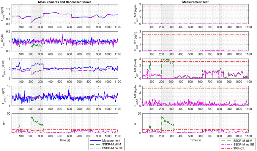
E1 SSDR-M framework results. Reconciled values and measurements (left) and global test and measurement test (right) in real-time. SSDR-M all M was reconciling with all measurements, SSDR-M no GE removes the gross error (gray area); the limit used was 99% confidence interval (C.I.)
On the right-hand set of plots in Fig. 5, the bottom figure shows the progress of the global test and the top three the measurement test results over time. Note that the measurement test failure occurs with the composition measurement. Therefore, the composition variable was removed from the reconciled values and added to the unmeasured variables for the period of times during which it failed (gray area). Reconciliation was executed again, and the global test passed from 200 to 328 s. If the global test had failed again, it would not be possible to reconcile because a lack of redundancy.
At around 100–200 s and between 600 and 820 s, there are small but frequent gross errors detected. In this example, these errors are caused by fluctuation in the composition measurement; the measurement test value for the composition (right-hand image in Fig. 5) proves it. Depending on the process limits, these might or might not have a significant effect. In this case, these fluctuations are believed to be due to fouling of the CDI probe at the exit of the first blender; a second measurement in another location might be needed for redundancy.
As can be seen in Fig. 6, the reconciled values obtained by the two approaches (when all four measurements are used, and gross errors are absent) are quite comparable. The global test also gives comparable results to the SPE, since both tests follow a chi-square distribution using a 99% interval. In the SSDR-D framework, the power contribution (absolute value) at time 200 s is 0.02 (%wt) for the API composition, while for the others, it is below 0.015 (kg/h). This information is comparable to the measurement test results. Both approaches indicate that the error is likely to lie in the composition measurement.
Fig. 6.
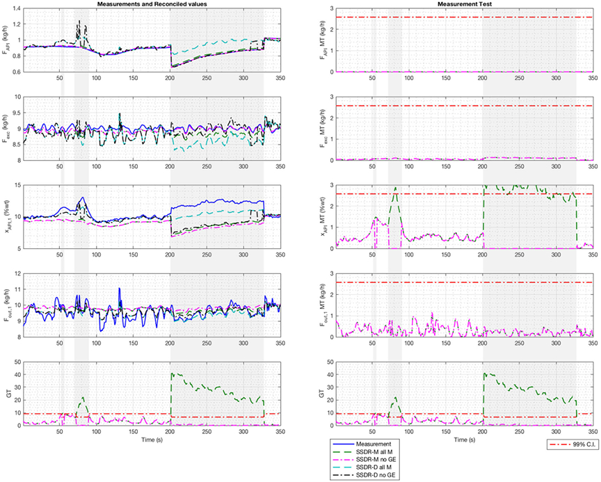
SSDR-D (PCA) and the SSDR-M framework results. SSDR-M all M is reconciling with all measurements, SSDR-M no GE removes the gross error when it is triggered (gray area), SSDR-D all M considering all measurements, and SSDR-D no GE removes the gross error (gray area)
In order to evaluate SSDR-M and SSDR-D results, we use Eq. 1, the value of the likelihood function, to compare the results (see Table 2). The first column shows the points of time for evaluation, which were randomly selected. In both cases, reconciliation was possible because there are at least three measurements active in the algorithm. If there was a gross error, it was located in the composition. If we compare the values of Eq. 1 for SSDR-D and SSDR-M, there is not one method that consistently gives a lower value of the likelihood function than the other. However, the material balance constraints (Eqs. 17 and 18) evaluated at the reconciled values obtained from SSDR-D, show deviations from zero, an indication that the reconciled values obtained via SSDR-D do not satisfy the mass balances and thus the lower values of Eq. 1 arise simply because these reconciled values are infeasible. In the case of the reconciled values obtained via SSDR-M, the constraints (Eqs. 17 and 18) have a maximum constraint tolerance of 1e-9 set in fmincon.
Table 2.
Objective function evaluation for E1 SSDR-M and SSDR-D
| Sample time (s) | Measurements in SSDR-M |
Measurements in SSDR-D |
SSDR-M Eq. 1 |
SSDR-D Eq. 1 |
SSDR-D Eq. 17 |
SSDR-D Eq. 18 |
|---|---|---|---|---|---|---|
| 3 | 4 | 4 | 1.93 | 8.10 | 0.18 | 0.04 |
| 30 | 4 | 4 | 3.30 | 6.54 | 0.18 | 0.03 |
| 38 | 4 | 4 | 2.10 | 1.82 | 0.18 | 0.03 |
| 92 | 4 | 4 | 5.56 | 6.70 | 0.18 | 0.03 |
| 141 | 4 | 4 | 3.46 | 2.82 | 0.18 | 0.03 |
| 271 | 3 | 3 | 0.02 | 0.06 | 0.18 | 0.02 |
| 280 | 3 | 3 | 0.01 | 0.57 | 0.18 | 0.02 |
| 286 | 3 | 3 | 0.01 | 0.66 | 0.18 | 0.02 |
| 304 | 3 | 3 | 0.01 | 0.56 | 0.18 | 0.02 |
| 337 | 4 | 4 | 0.07 | 2.03 | 0.19 | 0.03 |
Under the SSDR-M framework, the measurement with a gross error was discarded when the global test failed. This corresponded to the composition measurement, and so it was moved to the unmeasured variable set and estimated using re-reconciled values of the flows and the component balance equation. In the SSDR-D case, when the error was detected, the PCA model treated that measurement as a missing measurement and computed its value using the NIPALS algorithm. The error detection activates when the SPE tests fail, and the power contribution shows there is an error in the composition. Figure 6 also shows the SSDR-M and the SSDR-D results when gross errors arise. It is important to note that, under the SSDR-D approach, the SPE results shown are only of the input variables (SPEX). The reconciled values from SSDR-M and SSDR-D begin to differ only in the presence of the gross error for the variables where the gross error is located, while the API flow and excipient flow are still similar. Note that if an additional sensor were to fail (i.e., fouling, probe disconnection), it would no longer be possible to generate reconciled values because there would be no measurement redundancy in the system. Under these conditions, it is in general not likely that the variable values as measured would satisfy all of the equations of the process model exactly.
E2 Case I Results
The results for a run of E2 are shown in Fig. 7. In this run, there are no gross errors (using 99% confidence interval), and thus the two frameworks give very similar reconciliation results since the additional underlying relationships between the measured variables are linear. However, there are differences in the treatment of the unmeasured variables. In the SSDR-M approach under normal operating conditions, the model equations will generate values of the unmeasured variables from the reconciled measured variable values. However, in the SSDR-D approach, the training data consists only of measured values; thus, the corresponding PCA model cannot reflect information associated with the unmeasured variable. Therefore, to estimate the unmeasured variable, the PCA model must be augmented with equations (in this case a composition balance) in order to compute the unmeasured composition using the reconciled values of the measured variables. Of course, one can also add another composition measurement at the exit of the second blender. However, we can only estimate the output flow of the first blender through a mass balance (Eq. 17).
Fig. 7.
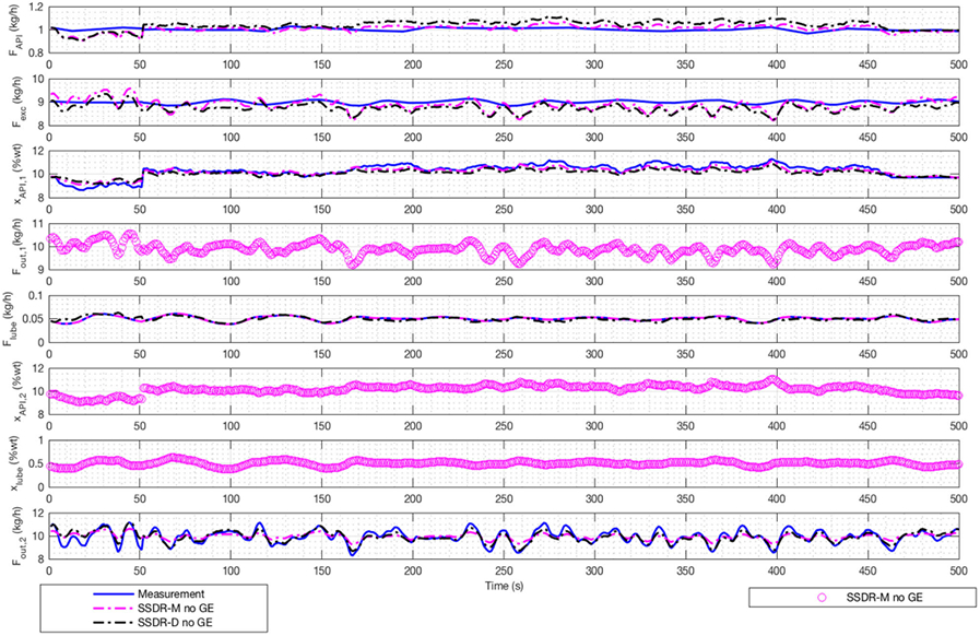
E2 case I framework results. SSDR-M and SSDR-D (PCA) reconciled values, unmeasured variables are marked as “o”
E2 Case II Results
In E2 case I, we are able to see how SSDR-M estimates unmeasured variables. However, we did not compare the performance between SSDR-M and SSDR-D. Since the data reported based on actual measurements (non-simulated data), the “true” values of the process variables are not known—they are only known within the limits of measurement errors. The objective of E2 case II is to show the importance of redundancy of measurements in comparing SSDR-M and SSDR-D results. For E2 case II, we added a composition measurement to increase redundancy. After analyzing the data from the pilot plant operation, we selected a period of time, where there were no gross errors; therefore, reconciled and measurement values were closed to each other. In the period of time from 11 to 110 s, we inserted a bias of + 3%wt in the second composition measurement offline (simulated scenario).
Figure 8 shows the reconciled values from SSDR-M and SSDR-D, with and without gross errors. Aside from the number of measurements and their location, the main difference between E1 and E2 is the way SSDR-D manages gross errors. In E1, if we have one gross error, it represented 25% of missing data; in E2, one gross error represents approximately 17% of missing data (satisfying the heuristic rule). SSDR-D all M denotes the results of reconciling with all measurements using PCA; in SSDR-D no GE when the gross error is triggered (gray area), the measurement with gross error is removed and is treated as a missing variable. The NIPALS algorithm is then used to estimate the value of that missing variable.
Fig. 8.
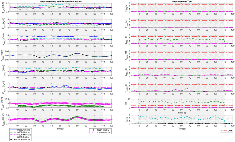
E2 case 2 SSDR-D (PCA) and the SSDR-M framework results. SSDR-M all M indicates the results of reconciliation with all measurements, SSDR-M no GE removes the gross error when it is triggered (gray area), SSDR-D all M considers all measurements, and SSDR-D no GE treats gross errors as missing measurements; unmeasured variables are marked as “o”
In the left-hand of Fig. 8, the reconciled values and measurements are shown. SSDR-D results show larger variations in the API flow and excipient flow than SSDR-M; while for the other variables, the SSDR-M and SSDR-D reconciled values are similar. At time 10 s, the global test and the SPE chart detect the injected error. The measurement test values suggest that the second API composition is likely at fault; this result is in accordance with the bias added in the measurement. This bias distorted the unmeasured variables estimates, especially the total flow estimated at the exit of the first blender. Nevertheless, the constraint values are not zero (see Table 3) for the SSDR-D solution, indicating some infeasibility. For SSDR-M, the maximum constraint tolerance is 1e-9. Moreover, Eqs. 18 and 22 give an estimate for unmeasured variables, such as the flow at the exit of the first blender and the lubricant composition.
Table 3.
Objective function evaluation for E2 case 2 SSDR-M and SSDR-D
| Sample time (s) | Measurements in SSDR-M |
Measurements in SSDR-D |
SSDR-M Eq. 1 |
SSDR-D Eq. 1 |
SSDR-D Eq. 19 |
SSDR-D Eq. 20 |
SSDR-D Eq. 21 |
|---|---|---|---|---|---|---|---|
| 5 | 6 | 6 | 0.31 | 11.50 | −0.06 | 0.11 | 0.02 |
| 6 | 6 | 6 | 0.19 | 8.11 | −0.06 | 0.12 | 0.03 |
| 13 | 5 | 5 | 1.19 | 59.11 | −0.05 | 0.10 | 0.07 |
| 34 | 5 | 5 | 0.82 | 8.81 | −0.04 | 0.07 | 0.03 |
| 39 | 5 | 5 | 0.67 | 12.42 | −0.05 | 0.04 | 0.01 |
| 46 | 5 | 5 | 0.16 | 9.36 | −0.05 | 0.10 | 0.03 |
| 53 | 5 | 5 | 0.62 | 5.35 | −0.07 | 0.13 | 0.02 |
| 84 | 5 | 5 | 1.43 | 3.18 | −0.03 | 0.14 | 0.07 |
| 92 | 5 | 5 | 0.44 | 17.55 | −0.04 | 0.09 | 0.05 |
| 96 | 5 | 5 | 0.56 | 22.29 | −0.04 | 0.08 | 0.04 |
| 99 | 5 | 5 | 0.57 | 19.50 | −0.04 | 0.08 | 0.04 |
| 114 | 6 | 6 | 1.56 | 2.21 | −0.04 | 0.09 | 0.03 |
Normally, in order to compare the two different approaches, SSDR-M and SSDR-D, we would use the actual value of the variables to compute the RMSE and residuals. In a simulated scenario, this would be the measurement before adding noise. In the E2 case II, we use actual measurements rather than simulations. Thus, in order to perform the comparison, we treat the measurement (before inserting the bias) as the point of comparison and treat it as the “actual value.” Table 4 represents the RMSE between the “actual value” and the reconciliation results. In this way, we can evaluate the performance of models in the presence of gross errors. In four variables out of six, SSDR-M gives the result closest to the measurement. For the composition at the exit of the second blender, SSDR-D is slightly better. Figure 9 shows the average absolute residual per model, based on Eq. 23, which uses the real measurement value (before inserting the bias) to evaluate performance. The lower the residual, the better the performance. In most of the variables, dealing with gross errors by treating them as unmeasured variables improves the estimated result. The flow measurement is the only exception. It should be noted that as expected, whether using the SSDR-M or SSDR-D, the variability, which results if gross errors are not eliminated, is very high.
| (23) |
where is a vector of measurements, is a vector of reconciled values, and r subscript stands for the real value.
Table 4.
Performance of SSDR-M and SSDR-D case 2
| Variable | NOC | RMSE SSDR-M no GE | RMSE SSDR-D no GE |
|---|---|---|---|
| FAPI (kg/h) | 1.00 | 7.61E–04 | 3.86E–02 |
| Fexc (kg/h) | 9.00 | 4.45E–02 | 1.74E–01 |
| xAPI,1a (% wt) | 10.15 | 2.94E–01 | 9.49E–01 |
| Flube (kg/h) | 0.02 | 1.39E–05 | 4.14E–05 |
| xAPI,2a (% wt) | 10.06 | 3.20E–01 | 2.31E–01 |
| Fout,2a (kg/h) | 9.66 | 5.80E–01 | 3.96E–01 |
Average using a window time of 10 s. Q was determined using the training data for the multivariate model
Fig. 9.
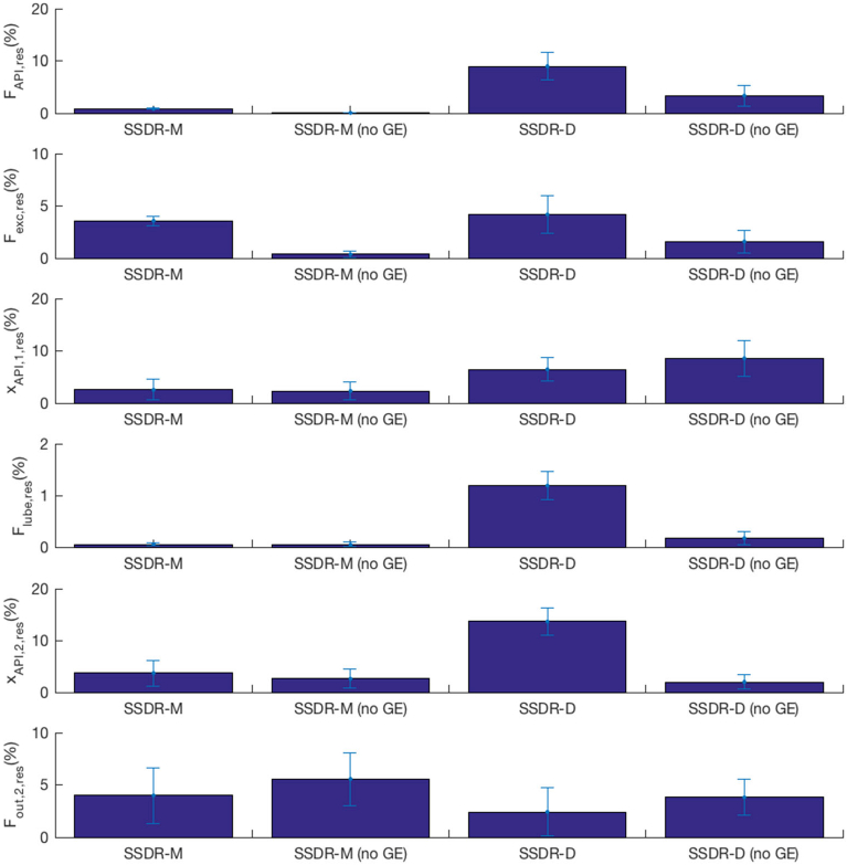
Average performance of SSDR-M and SSDR-D in the presence of gross errors (GE)
Conclusions
Data reconciliation and gross errors detection in real time are important for the effective operation of a production line given that the online sensors invariably have significant measurement error. The SSDR-M framework proves to be an efficient way to determine the most likely value of process variables and to identify gross errors during operation. Providing the sensor network has measurement redundancy, the reconciled values are preferred to the raw measurements for use in effective process monitoring and control.
In the simple case studies reported here, the distortion in the reconciled variables resulting from the presence of gross errors is readily observed. However, the ability to effectively predict process variables in the presence of gross errors is dependent on measurement redundancy in the sensor network. This, of course, imposes equipment and operating cost in the process. For the direct compression continuous tableting line, it is imperative that additional PAT tools be introduced for the remaining CQA’s and CPP’s [41], for instance, online measurement of tablet hardness and weight or the deployment of PAT tools for powder flow. In continuing work in our team, these are being investigated.
As confirmed in this work, an SSDR-D approach which uses multivariate statistical models can generate reconciliation results equivalent to those obtained via SSDR-M under appropriate conditions: specifically, if the relationships between the measured variables are linear and n-k principal components are used. The reconciled values will differ, when nonlinearities arise, such as when the tablet property measurements used in the model associated with the tablet press are added to the reconciliation problem. In terms of gross error detection for the SSDR-D approach, the SPE criterion gives results comparable to the global test used in SSDR-M, since by definition both instances follow a chi-squared distribution. The SSDR-M measurement test gives comparable results to the power contribution used in SSDR-D in these case studies. However, at this point, we have not confirmed that they are strictly speaking statistically equivalent. The two approaches also differ in the manner of treatment of unmeasured variables. In the SSDR-M approach, unmeasured variables simply are accommodated as dependent variables in the process model. In the SSDR-D approach, unmeasured variables can only be estimated if the PCA model is supplemented with appropriate mechanistic equations relating the unmeasured variables to the reconciled measured variables.
Acknowledgments
The authors will like to thank, Benjamin Rentz for his collaboration in the experimental procedure, Joonyoung Yu and Dr. Marcial Gonzalez for the design of the CDI-NIR holder, Dr. Salvador Garcia-Munoz for providing the “phi” latent variable modeling toolbox (version 1.7), Sudarshan Ganesh for his feedback in the design of experiments, and Yash D. Shah and James Wiesler for their continuous support in the project.
Funding Information
Funding for this project was made possible, in part, by the Food and Drug Administration through grant U01FD005535; views expressed by authors do not necessarily reflect the official policies of the Department of Health and Human Services nor does any mention of trade names, commercial practices, or organization imply endorsement by the US Government. This work was also supported in part by the National Science Foundation under grant EEC-0540855 through the Engineering Research Center for Structure Organic Particulate Systems.
Appendix
Experimental Procedure and Information Flow
The experimental procedures for executing runs for cases E1 and E2 are quite straightforward. A run is initiated by turning on feeders 1 and 2, which take 1–2 min to arrive at steady state as defined by the conditions shown in Table 1. With the blender operating at 200 rpm, an additional period 2–3 min was allowed from the moment the feeders reached steady state [42] before reconciliation was initiated, corresponding to reaching a Q at or below the values in Table 1. In case E1, the process set points are as shown in Table 1. The measurements are collected and sent to MATLAB-2016a-64bit for execution, as shown in the system configuration (Appendix Fig. 10). During the runs, all variables are saved in the Emerson DeltaV v.13.3 process historian, operating using two Dell Precision T1700 64-bit computers with Windows 2008 RL2, configured as five virtual computers. The first server houses App Station (AS), ProPlus (PP), and Terminal Server 1 (TS1). The second server houses Engineering Station (ENG) and Terminal Server 2 (TS2). As configured, each virtual computer has a specific function: the ENG station is used for adding equipment and troubleshooting issues. Computer AS is used when other applications, such as MATLAB, need to communicate with the DeltaV system. The PP computer is used to add any figures in the main template for the operation of the pilot plant, process historian view diagrams, and to add or modify the control modules in DeltaV. Finally, TS1 and TS2 are used to operate the process.
Fig. 10.
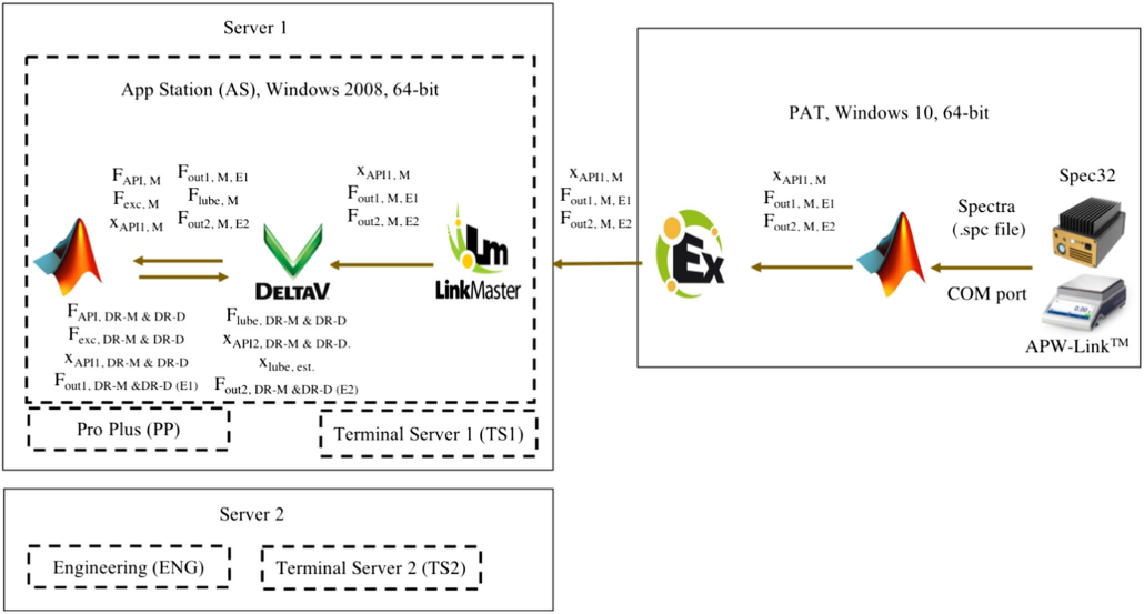
System configuration for the continuous tableting line: virtual computers (−) and physical computer (−)
The codes for the SSDR-M and the SSDR-D frameworks are implemented in MATLAB 2015b 32-bit and installed in the AS computer. Since MATLAB serves as a client, by using the OPC toolbox, the code reads the measured flows and composition from the DeltaV historian, solves the optimization problem, and writes the information directly into the DeltaV control module “SSDR.” All control modules and process historian view diagrams were created on the PP computer. For these experiments, the system was operated from the TS1 computer.
Another, physical computer: Dell Inspiron Windows 10 64-bit laptop using Intel Core™ i7 and 8 GB RAM called “PAT,” is used to connect to the necessary PAT tools, such as the CDI-NIR or the Mettler Toledo balance, and to link the required information to the other computers. All composition and flow measurements are in the DeltaV historian. However, it has to be noted, that of these four subsystem measurements, only the feeder flow values are directly sent to the DeltaV system. For the composition measurements, the CDI-NIR is connected via USB port to the “PAT” computer. By using the CDI-NIR software, called Spec32, the spectra measurement is collected as a “.spc file.” This file is generated every second and read by the multivariate statistical methods code. The code, which is in MATLAB 2016a 64-bit, executes the PLS model, created in “phi” software package and loaded as a “.mat” file. This software was acquired through personal communication with Dr. Garcia-Munoz. The results are sent to KEPServerEX v6. This server, provided by Kepware, sends the information to LinkMaster v3, which is connected to the DeltaV system. In parallel, the mass flow MATLAB code is executed using the “parpool” function. This code calls the information from the APW-Link™ software, which is connected to the Mettler Toledo balance through a COM port. It is important to mention that the acetaminophen composition and mass flow measurements are computed using an averaging time window of 10 s.
References
- 1.U. S. D. of H. and H. S. FDA, Guidance for industry PAT—a framework for innovative pharmaceutical development, manufacturing, and quality assurance, no. September, p. 16; 2004. [Google Scholar]
- 2.Ierapetritou M, Muzzio F, Reklaitis GV. Perspectives on the continuous manufacturing of powder-based pharmaceutical processes. AICHE J. 2016;62(6):1846–62. [Google Scholar]
- 3.Lee SL, O’Connor TF, Yang X, Cruz CN, Chatterjee S, Madurawe RD, et al. Modernizing pharmaceutical manufacturing: from batch to continuous production. J Pharm Innov. 2015;10(3):191–9. [Google Scholar]
- 4.Su Q, Moreno M, Giridhar A, Reklaitis GV, Nagy ZK. A systematic framework for process control design and risk analysis in continuous pharmaceutical solid-dosage manufacturing. In: J. Pharm. Innov, vol. 12; 2017. p. 327–46. [Google Scholar]
- 5.Knopf C. Introduction to data reconciliation and gross error detection. In: Modeling, analysis and optimization of process and energy systems. Hoboken: Wiley; 2011. [Google Scholar]
- 6.Narasimhan S, Jordache C. Data reconciliation and gross error detection. Houston: Gulf Publishing Company; 2000. [Google Scholar]
- 7.Alhaj-Dibo M, Maquin D, Ragot J. Data reconciliation: a robust approach using a contaminated distribution. Control Eng Pract. 2008;16(2):159–70. [Google Scholar]
- 8.Tong H. Studies in data reconciliation using principal component analysis. Ph.D. Thesis. Hamilton: McMaster University; 1995. [Google Scholar]
- 9.Cencic O, Fruhwirth R. A general framework for data reconciliation—part I: linear constraints. Comput Chem Eng. 2015;75:196–208. [Google Scholar]
- 10.Narasimhan S, Bhatt N. Deconstructing principal component analysis using a data reconciliation perspective. Comput Chem Eng. 2015;77:74–84. [Google Scholar]
- 11.Narasimhan S, Shah SL. Model identification and error covariance matrix estimation from noisy data using PCA. Control Eng Pract. 2008;16(1):146–55. [Google Scholar]
- 12.Benqlilou C. Data reconciliation as a framework for chemical processes optimization and control. Doctoral thesis, Universitat Politècnica de Catalunya; 2004. [Google Scholar]
- 13.Diehl M, Bock HG, Schlöder JP, Findeisen R, Nagy Z, Allgöwer F. Real-time optimization and nonlinear model predictive control of processes governed by differential-algebraic equations. J Process Control. 2002;12:577–85. [Google Scholar]
- 14.Liu J, Su Q, Moreno M, Laird C, Nagy Z, Reklaitis G. Robust state estimation of feeding–blending systems in continuous pharmaceutical manufacturing. Chem Eng Res Des. 2018;134:140–53. [DOI] [PMC free article] [PubMed] [Google Scholar]
- 15.Bai S, Thibault J, McLean DD. Dynamic data reconciliation: alternative to Kalman filter. J Process Control. 2006;16(5):485–98. [Google Scholar]
- 16.Haseltine EL, Rawlings JB. Critical evaluation of extended Kalman filtering and moving-horizon estimation. Ind Eng Chem Res. 2005;44(8):2451–60. [Google Scholar]
- 17.Crowe CM, Campos YAG, Hrymak A. Reconciliation of process flow rates by matrix projection. Part I: linear case. AICHE J. 1983;29(6):881–8. [Google Scholar]
- 18.Arora N, Biegler LT. Redescending estimators for data reconciliation and parameter estimation. Comput Chem Eng. 2001;25(11):1585–99. [Google Scholar]
- 19.Almaya A, De Belder L, Meyer R, Nagapudi K, Lin H-RH, Leavesley I, et al. Control strategies for drug product continuous direct compression—state of control, product collection strategies, and startup/shutdown operations for the production of clinical trial materials and commercial products. J Pharm Sci. 2017;106(4):930–43. [DOI] [PubMed] [Google Scholar]
- 20.Jackson JE. A user’s guide to principal components. New York: Wiley; 1991. [Google Scholar]
- 21.Tong H, Crowe CM. Detection of gross erros in data reconciliation by principal component analysis. AICHE J. 1995;41(7):1712–22. [Google Scholar]
- 22.MacGregor J, Cinar A. Monitoring, fault diagnosis, fault-tolerant control and optimization: data driven methods. Comput Chem Eng. 2012;47:111–20. [Google Scholar]
- 23.Wold S, Sjöström M, Eriksson L. PLS-regression: a basic tool of chemometrics. Chemom Intell Lab Syst. 2001;58(2):109–30. [Google Scholar]
- 24.Kourti T, MacGregor JFJF. Process analysis, monitoring and diagnosis, using multivariate projection methods. Chemom Intell Lab Syst. 1995;28(1):3–21. [Google Scholar]
- 25.Imtiaz SA, Shah SL, Narasimhan S. Missing data treatment using iterative PCA and data reconciliation. IFAC Proc Vol. 2004;37(9):197–202. [Google Scholar]
- 26.Nelson PRC, Taylor PA, MacGregor JF. Missing data methods in PCA and PLS: score calculations with incomplete observations. Chemom Intell Lab Syst. 1996;35(1):45–65. [Google Scholar]
- 27.Folch-Fortuny A, Arteaga F, Ferrer A. PCA model building with missing data: new proposals and a comparative study. Chemom Intell Lab Syst. 2015;146:77–88. [Google Scholar]
- 28.Kim I-W, Kang MS, Park S, Edgar TF. Robust data reconciliation and gross error detection: the modified MIMT using NLP. Comput Chem Eng. 1997;21(7):775–82. [Google Scholar]
- 29.Gupta A, Giridhar A, Venkatasubramanian V, Reklaitis GV. Intelligent alarm management applied to continuous pharmaceutical tablet manufacturing: an integrated approach. Ind Eng Chem Res. 2013;52(35):12357–68. [Google Scholar]
- 30.MacGregor JF, Yu H, García Muñoz S, Flores-Cerrillo J. Data-based latent variable methods for process analysis, monitoring and control. Comput Chem Eng. 2005;29(6):1217–23. [Google Scholar]
- 31.Hotelling H. The generalization of Student’s ratio. Ann Math Stat. 1931;2(3):360–78. [Google Scholar]
- 32.Miller P, Swanson RE, Heckler CE. Contribution plots: a missing link in multivariate quality control. Appl Math Comput Sci. 1998;8:775–92. [Google Scholar]
- 33.Le Roux GAC, Santoro BF, Sotelo FF, Teissier M, Joulia X. Improving steady-state identification. Comput Aided Chem Eng. 2008;25:459–64. [Google Scholar]
- 34.Bagajewicz MJ, Chmielewski DJ, Tanth DN. Smart process plants: software and hardware solutions for accurate data and profitable operations, 1st edn. New York: McGraw-Hill Education; 2010. [Google Scholar]
- 35.Cao S, Rhinehart RR. An efficient method for on-line identification of steady state. J Process Control. 1995;5(6):363–74. [Google Scholar]
- 36.Nomikos P, MacGregor JF. Multivariate SPC charts for monitoring batch processes. Technometrics. 1995;37(1):41–59. [Google Scholar]
- 37.Parikh DM. Handbook of pharmaceutical granulation technology, 3rd edn. In: Drugs and the pharmaceutical sciences, volume 198. New York: Informa Healthcare USA; 2010. [Google Scholar]
- 38.Austin J, Gupta A, McDonnell R, Reklaitis GV, Harris MT. A novel microwave sensor to determine particulate blend composition on-line. Anal Chim Acta. 2014;819:82–93. [DOI] [PubMed] [Google Scholar]
- 39.Vanarase AU, Alcalà M, Jerez Rozo JI, Muzzio FJ, Romañach RJ. Real-time monitoring of drug concentration in a continuous powder mixing process using NIR spectroscopy. Chem Eng Sci. 2010;65(21):5728–33. [Google Scholar]
- 40.García-Muñoz S. Phi MATLAB toolbox. Personal communication; 2015. [Google Scholar]
- 41.Ganesh S, Troscinski R, Schmall N, Lim J, Nagy Z, Reklaitis G. Application of X-ray sensors for in-line and noninvasive monitoring of mass flow rate in continuous tablet manufacturing. J Pharm Sci. 2017;106:3591–603. [DOI] [PubMed] [Google Scholar]
- 42.Vanarase AU, Muzzio FJ. Effect of operating conditions and design parameters in a continuous powder mixer. Powder Technol. 2011;208(1):26–36. [Google Scholar]