Functional mixed effects clustering with application to longitudinal urologic chronic pelvic pain syndrome symptom data

Abstract

By clustering patients with the urologic chronic pelvic pain syndromes (UCPPS) into homogeneous subgroups and associating these subgroups with baseline covariates and other clinical outcomes, we provide opportunities to investigate different potential elements of pathogenesis, which may also guide us in selection of appropriate therapeutic targets. Motivated by the longitudinal urologic symptom data with extensive subject heterogeneity and differential variability of trajectories, we propose a functional clustering procedure where each subgroup is modeled by a functional mixed effects model, and the posterior probability is used to iteratively classify each subject into different subgroups. The classification takes into account both group-average trajectories and between-subject variabilities. We develop an equivalent state-space model for efficient computation. We also propose a cross-validation based Kullback-Leibler information criterion to choose the optimal number of subgroups. The performance of the proposed method is assessed through a simulation study. We apply our methods to longitudinal bi-weekly measures of a primary urological urinary symptoms score from a UCPPS longitudinal cohort study, and identify four subgroups ranging from moderate decline, mild decline, stable and mild increasing. The resulting clusters are also associated with the one-year changes in several clinically important outcomes, and are also related to several clinically relevant baseline predictors, such as sleep disturbance score, physical quality of life and painful urgency.

1. Introduction

Cluster analysis has been widely used to identify subgroups in heterogeneous populations. In recent years, this technique has been extended to functional data analysis settings (See Jacques and Preda, 2014 for a review). In this paper, we propose a functional mixed effects clustering algorithm, in which each potential subgroup is modeled by a functional mixed effects model (Guo, 2002). Unlike the existing methods, our proposed classification algorithm allows for nested structures, and takes into account both group-average trajectories and between-subject variabilities in calculating the posterior probability of cluster membership. We also propose a cross-validation Kullback-Leibler information criterion to select the optimal number of clusters.

This research was motivated by the complex analytical challenges of subgroup discovery within a multicenter clinical research network, aiming to identify differential trajectories of longitudinal symptom profiles, in the presence of differential within-patient variability of symptoms. The National Institute of Diabetes and Digestive and Kidney Diseases (NIDDK) launched a multicenter clinical research network labeled “Multidisciplinary Approach to the Study of Chronic Pelvic Pain (MAPP)” (http://www.mappnetwork.org/) in 2008, as a novel effort to better understand the pathophysiology of urologic chronic pelvic pain syndrome (UCPPS), a multifactorial constellation of symptoms characterized by one or more types and locations of urologic pain (bladder, genital), urinary urgency and/or urinary frequency symptoms. Due to extensive symptom heterogeneity and differential longitudinal variability of symptom presentations, previous decades of well-conducted NIDDK-funded cohort studies (1992–2003) and clinical trials (1998–2008) were inconclusive in identifying improved approaches to the clinical management of UCPPS patients. These patient-reported symptom data were obtained from the Epidemiology and Phenotyping Study (EPS), a prospective observational cohort study of men and women with UCPPS conducted within MAPP Clinical Research Network (Clemens et al., 2014). The impact and burden of UCPPS symptoms are substantial. Patients suffer considerable morbidity resulting in a significant decrease in quality of life for both the patient, and his/her partner due to the physical and psychological impact of the condition. In fact, the quality of life of these patients has been characterized as being worse than that of patients undergoing hemodialysis (Held et al., 1990). In the U.S., the prevalence of UCPPS symptoms has been estimated to be between 1.8% to 6.4%, depending upon case definitions and screening methods (Berry et al., 2011; Suskind et al., 2013). Despite intensive study over the past decade, clinical trials have failed to identify effective therapies, and basic science studies have failed to identify specific pathophysiology for these conditions (Clemens et al., 2014).

One of the biggest challenges in treating patients with UCPPS is the lack of understanding of the etiology and pathophysiology underlying the condition. All treatments are empiric because we do not have a clear target for therapy (Pontari, 2013). Previous attempts in NIH cohorts of patients with pelvic pain could not identify baseline demographic or clinical factors that predicted symptom changes over time (Propert et al., 2006). If we are able to cluster the population into homogeneous subgroups and gain insight into the propensity for changes in symptoms, we will be able to look for what etiologic factors are driving the pain and urinary symptoms, and may be responsible for the propensity to get better or worse. These factors include both other longitudinal clinical outcomes and baseline predictors. The MAPP project was set up to better understand the underlying causes of UCPPS symptoms by conducting deep clinical phenotyping, pain sensitivity testing, neuroimaging and biospecimen analyses to explore the complexity of biological processes in a patient with chronic pelvic pain. In particular, the resultant chronic pelvic pain, urinary urgency and voiding symptoms in UCPPS patients are likely the result of widely heterogeneous processes in different subgroups of patients. By identifying the risk factors associated with a patient’s improvement or worsening, we hope to uncover new understanding of the pathogenesis of UCPPS, which may ultimately guide targeted therapies for targeted subgroups of UCPPS patients.

One of the primary aims of the MAPP EPS was to characterize distinguishable longitudinal urological and non-urological symptom patterns, and to further investigate clinical, biological and psychosocial risk factors associated with these symptom patterns. In this longitudinal cohort study, 424 UCPPS participants provided self-reported biweekly symptom data via web-based tools for 48 weeks. Each participant also returned for extensive in-clinic visits at 24 weeks and 48 weeks (Landis et al., 2014). Griffith et al. (2016) used exploratory factor analyses and identified that two factors, pelvic pain severity and urinary symptoms severity, provided the best psychometric description of items contained in the questionnaires. Their results suggested that pelvic pain and urinary symptoms should be assessed separately, rather than combined into one total score. Total scores that combine the separate factors of pain and urinary symptoms into one score may be limited for clinical and research purposes. In this paper, we focus on clustering the longitudinal urinary symptoms severity index, a scale ranging from 0 to 25, where 0 indicates no urgency and 25 indicates the most severe urgency. As reported in Stephens-Shields et al. (2016), these UCPPS symptoms are prone to regression-to-the-mean (RTM) effects, so the urinary symptoms severity scores for week 0 and 2 were excluded from the functional clustering algorithm utilized to form subgroups with distinct patterns of longitudinal trajectories. We further subtract the week 4 (visit 3) data from the data at weeks 4 to 48 to create the changes of the urinary severity index. Figure 1 shows different subgroups of participant trajectories of their urinary symptoms severity changes over time (visits 3, ⋯, 25). We can see that the subgroups can differ in terms of both mean trajectories and variabilities over time. It is desirable for the clustering algorithm to be able to capture these complex differential trajectories over time, and take into account the differential within-cluster variability.

Figure 1:

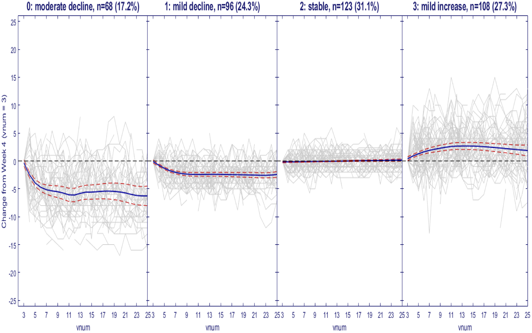
Trajectories of changes of urinary severity relative to Week 4 together with the estimated group-averages. Decreasing scores suggest that patients are improving over time and increasing scores suggest worsening (Gray solid line, raw data; Blue solid line, mean-curve estimates; red dashed lines, 95% Bayesian confidence bands)

In recent years, many alternative methods for functional clustering have been proposed, as summarized recently by Jacques and Preda (2014) into four different approaches. The first approach consists of raw-data methods working directly on the evaluation points of the curves, but ignoring the functional features of the data. The second general approach consists of distance-based methods using specific distances for the functional data. The L₂ metric is a widely used distance measure, which can be combined with the k-means algorithm (Ieva et al., 2013, Tokushige et al., 2007). Ferraty and Vieu (2006) extended the k-mean algorithm to a hierarchical clustering setting. Other distance measures like Pearson’s correlation coefficients and related distances were used in Golay et al. (1998). The third functional clustering approach includes filtering methods which first approximate the curves into a finite basis of functions, and then perform the functional clustering using the basis expansion coefficients(e.g. Abraham et al., 2003, Peng and Muller, 2008, Kayano et al., 2010). The main limitation of these filtering methods is that the variability in the dimension reduction step is not taken into account in the clustering step. The fourth approach to functional clustering performs simultaneously dimensionality reduction of the curves and clustering. The basis expansion coefficients are considered as random variables having a cluster-specific probability distribution, and the clustering is model-based (e.g. James and Sugar, 2003, Heard et al., 2006, Ray and Mallick, 2006, Giacofci et al., 2013, Chiou and Li, 2007, and Jacques and Preda, 2013). However, none of these four approaches explicitly accommodate both the within-cluster variations and cluster-average profiles in the clustering. There are two main approaches in model based clustering in general (Ganesalingam, 1989). The first approach is based on mixture models and estimated through EM algorithm or Bayesian methods. This approach only estimates the probabilities that a unit belongs to all the possible subgroups, without actually classifying the unit into one of the subgroups. Both group-average profiles and cluster memberships are estimated from the overall mixture models and are difficult to interpret as specific to certain subgroups. Another approach is based on classification, where the unit is iteratively assigned to one of the subgroups. The group-average profiles are estimated based on the subjects within the subgroups and the cluster memberships have clear interpretations. Since our final interest is to separate the population into more homogeneous subgroups, we adopt the classification approach.

In this paper, we propose a functional mixed effects clustering algorithm. We model each sub-group by a functional mixed effects model (Guo, 2002), in which both the group-average profiles and the subject-specific functional random deviations are modeled by smoothing splines. The classification algorithm is then based on the posterior probability of a subject belonging to a specific cluster, and the subject is assigned into the cluster with the maximum posterior probability. This proposed new method accounts for both the within-group trajectories and between-subject variability, and can handle sparse data. The calculation of the posterior probability of the new subject belonging to a specific cluster requires the calculation of the conditional distribution for each potential subgroup of the new subject conditional on all other subjects in that subgroup. We show that it can be computed as the ratio of the likelihoods, with and without, the new subject added to the subgroup. We exploit the state space representation of the functional mixed effects model (Guo, 2002) for computation efficiency and the resultant algorithm is in the linear order of the total number of observations, N.

Another key issue in clustering is to determine the number of clusters. In this context of model-based functional clustering of longitudinal data, penalized likelihood methods provide a general framework to optimally estimate the number of clusters. The Akaike Information Criterion (AIC), Bayesian Information Criterion (BIC), and the Integrated Completed Likelihood (ICL) (Biernacki et al., 2000) are most commonly used (e.g. Ciampi et al., 2012, Luan and Li, 2003, McNicholas and Murphy, 2010, Baudry, 2015). These model selection criteria are shown to be effective in the situation without nested structures. However, it is shown that the effective degrees of freedom in these penalized likelihood criteria, such as AIC and BIC, in the hierarchical and more complex settings are difficult to calculate (Vaida and Blanchard, 2005, Liang et al., 2008, Greven and Kneib, 2010), and many direct extensions of these methods to functional clustering models may not be valid. In this paper, we propose a leave-one-subject-out Kullback-Leibler criterion (Kullback and Leibler, 1951) to select the number of clusters. The criterion reduces to predictive classification log-likelihood and can be directly calculated after the clustering algorithm converges without extra model fitting.

The remainder of this article is organized as follows. We propose the functional mixed effects clustering procedure in Section 2. We then apply the methods to the MAPP longitudinal symptom data in Section 3, and investigate the finite sample performance through simulations in Section 4. Some concluding remarks are offered in Section 5.

2. Functional mixed effects clustering algorithm

In this section, we first introduce the K-class mixture functional mixed effects model which is the backbone of the clustering algorithm. We then cast it into a state space form so that existing Kalman filtering and smoothing algorithms can be used to efficiently fit the model. From the state space model, we can efficiently compute the posterior probability of a new subject belonging to a given subgroup that enables us to iteratively cluster the subjects into different subgroups. A cross-validation Kullback-Leibler criterion is proposed to select the optimal number of sub-groups.

2.1. K-class Mixture Function Mixed Effect Model

For simplicity, we assume the observational time does not depend on the cluster. Following the standard approaches in functional data analysis, we first map the range of observational time to [0, 1]. For k, k = 1, 2, …, K, we assume the kth sub-group has the following functional mixed effects model:

$$y_{ijk}=X_{ij}{\beta }^{(k)}\left(t_{ij}\right)+Z_{ij}{\alpha }_i^{(k)}\left(t_{ij}\right)+e_{ijk},e_{ijk}~N\left(0,{\sigma }_{ek}^2\right)$$ (1)

where y_ijk is the jth observation observed at t_ij from the ith subject in the kth cluster $\left(i=1,2,\dots ,n_k,j=1,2,\dots ,m_i,{\sum }_{k=1}^K{n}_k=N\right)$, i) ${\beta }^{(k)}(t)={\left\{{\beta }_1^{(k)}(t),\dots ,{\beta }_p^{(k)}(t)\right\}}^T$ is p × 1 vector of functional fixed effects; ii) ${\alpha }_i^{(k)}(t)={\left\{{\alpha }_{i1}^{(k)}(t),\dots ,{\alpha }_{iq}^{(k)}(t)\right\}}^T$ is a q × 1 vector of functional random effects, which are modeled as realizations of q × 1 vector of zero mean Gaussian process $A(t)={\left\{a_1^{(k)}(t),\dots ,a_q^{(k)}(t)\right\}}^T$; iii) X_ij = {X_ij(1), …, X_ij(p)}(1 × p) and Z_ij = {Z_ij(1), …, Z_ij(q)}(1 × q) are design matrices for the fixed and random effects, respectively; and iv) e_ijk is the independent and identically normally distributed measurement error. Similar to the interpretation of linear mixed effects models in the longitudinal settings, β^(k)(t) can be interpreted as population-average profile for cluster k, $Z_{ij}{\alpha }_i^{(k)}(t)$ as the ith curve-specific deviation from the population-average profiles, and $X_{ij}{\beta }^{(k)}(t)+Z_{ij}{\alpha }_i^{(k)}(t)$ as the ith subject-specific function given in cluster k. These models are natural extensions of linear mixed effects models to functional data and can incorporate complex designs. By using flexible functional random effects to take into account the corresponding correlation structures, we can also use the correct source of variations in the classification.

2.2. State Space Representation

Model (1) can be represented into a multivariate state space model. Given the construction is the same for different clusters, we will suppress the superscript (k) in this section. To simplify the presentation, we assume that observations on different series were collected at the same design points T = {t₁, …, t_M}, m_i ≤ M, j = 1, …, M, and δt_j = t_j − t_j−1, t₀ = 0. When the subjects have different design points, we can choose a finer grid to ensure all the observational time points are covered. Since the calculation is only needed at time points with data, this finer grid does not create an extra burden in computation.

For the fixed functional effects, we want them to be pure data driven and use the cubic spline model of Wecker and Ansley (1983), with diffuse priors at t = 0. Denote ${\beta }_v^{\prime }(t)$ as the derivative of β_v(t), for v = 1, ⋯, p, we can have the equivalent state equation for each element of β(t) as:

$$\left(\begin{array}{l}{\beta }_v\left(t_j\right)\hfill \\ {\beta }_v^{\prime }\left(t_j\right)\hfill \end{array}\right)=H_{vj}\left(\begin{array}{l}{\beta }_v\left(t_{j-1}\right)\hfill \\ {\beta }_v^{\prime }\left(t_{j-1}\right)\hfill \end{array}\right)+w_{vj},w_{vj}~N\left(0,W_{vj}\right),$$

where the transition matrix and perturbation variance-covariance matrix are: $H_{vj}=\left[\begin{array}{cc}1& \delta t_j\\ 0& 1\end{array}\right]$, $W_{vj}={\lambda }_b^{-1}\left[\begin{array}{cc}\delta t_j^3/3& \delta t_j^2/2\\ \delta t_j^2/2& \delta t_j\end{array}\right]$, The initial values at t = 0 are modeled as ${\left\{{\beta }_v(0),{\beta }_v^{\prime }(0)\right\}}^T~N(0,\tau I)$ with τ → ∞.

For the random functional effects, the regular random cubic spline model tends to lead to larger between-subject variances over time as it is non-stationary. A stationary functional random effects model such as a periodic cubic spline of Qin and Guo (2006) is too restrictive as it can not allow the between-subject variability to change over time. We therefore adopt a L−spline approach of Ansley et al. (1993) and use a sin function prior to construct the corresponding state space model, which has the flexibility to handle the time-varying variabilities but does not lead to larger and larger confidence intervals over time. By putting the penalty on L_tα_i(t), where L_t = d²/dt²+(2π)², the null space contains cos(2πt) and sin(2πt) and penalty part of the random functional effect represents smooth deviations from the null space controlled by the smoothing parameter. Following the derivation of Qin (2004), we can have the equivalent state equation for each element of α_i(t) as:

$$\left(\begin{array}{c}{\alpha }_{il}\left(t_j\right)\\ {\alpha }_{il}^{\prime }\left(t_j\right)\end{array}\right)=H_{ilj}\left(\begin{array}{c}{\alpha }_{il}\left(t_{j-1}\right)\\ {\alpha }_{il}^{\prime }\left(t_{j-1}\right)\end{array}\right)+w_{ilj},w_{ilj}~N\left(0,W_{ilj}\right),$$

where the transition matrix and perturbation variance-covariance matrix are:

$$H_{ilj}=\left[\begin{array}{cc}\text{cos}2\pi \delta t_j& \frac{1}{2\pi }\text{sin}2\pi \delta t_j\\ -2\pi \text{sin}2\pi \delta t_j& \text{cos}2\pi \delta t_j\end{array}\right],W_{ilj}={\lambda }_a^{-1}\left[\begin{array}{cc}\frac{1}{8{\pi }^2}\delta t_j-\frac{1}{32{\pi }^3}\text{sin}4\pi \delta t_j& \frac{1}{16{\pi }^2}\left(1-\text{cos}4\pi \delta t_j\right)\\ \frac{1}{16{\pi }^2}\left(1-\text{cos}4\pi \delta t_j\right)& \frac{1}{8\pi }\text{sin}4\pi \delta t_j+\frac{\delta t_j}{2}\end{array}\right].$$

The initial values at t = 0 are modeled as ${\left\{{\alpha }_{il}(0),{\alpha }_{il}^{\prime }(0)\right\}}^T~N(0,D(\gamma ))$, where γ are unknown parameters.

We can stack all the subjects together to create a vector state space model. Denote $Y_j={\left\{y_{1j},\dots ,y_{n_{k}j}\right\}}^T$, $e_j={\left\{e_{1j},\dots ,e_{n_{k}j}\right\}}^T$, ${\beta }^{*}\left(t_j\right)={\left\{{\beta }_1\left(t_j\right),{\beta }_1^{\prime }\left(t_j\right),\dots ,{\beta }_p\left(t_j\right),{\beta }_p^{\prime }\left(t_j\right)\right\}}^T$, ${\alpha }_i^{*}\left(t_j\right)={\left\{{\alpha }_{i1}\left(t_j\right),{\alpha }_{i1}^{\prime }\left(t_j\right),\dots ,{\alpha }_{iq}\left(t_j\right),{\alpha }_{iq}^{\prime }\left(t_j\right)\right\}}^T$. ${\alpha }^{*}\left(t_j\right)=\left\{{\alpha }_1^{*T}\left(t_j\right),\dots ,{\alpha }_{n_k}^{*T}\left(t_j\right)\right\}$, $x\left(t_j\right)={\left\{{\beta }^{*T}\left(t_j\right),{\alpha }^{*T}\left(t_j\right)\right\}}^T$. We then define n_k × 2(n_k × q + p) observational matrix with the form $F_j=\left\{{\left(X_{1j}^{*T},\dots ,X_{n_{k}j}^{*T}\right)}^T,\text{diag}\left(Z_{1j}^{*},\dots ,Z_{n_{k}j}^{*}\right)\right\}$, where diag means the diagonal matrix, $X_{ij}^{*}$ and $Z_{ij}^{*}$ are design matrices X_ij and Z_ij with the columns corresponding to the derivatives augmented by zeros, i.e., $X_{ij}^{*}(2v-1)=X_{ij}^{*}(v)$, $X_{ij}^{*}(2v)=0$ for v = 1, …, p and, $Z_{ij}^{*}(2l-1)=Z_{ij}^{*}(l)$, $Z_{ij}^{*}(2l)=0$ for l = 1, …, q; define $w_j={\left(w_{1j}^T,\dots ,w_{pj}^T,w_{11j}^T,\dots ,w_{n_{k}qj}^T\right)}^T$, 2(n_k×q+p) × 2(n_k×q+p) transition matrix with the form $H_j=\text{diag}\left(H_{1j},\dots ,H_{pj},H_{11j},\dots ,H_{n_{k}qj}\right)$, the 2(n_k×q+p) × 2(n_k×q+p) perturbation variance-covariance matrix with the form $W_j=\text{diag}\left(W_{1j},\dots ,W_{pj},W_{11j},\dots ,W_{n_{k}qj}\right)$. Stacking all the functional effects into a multivariate vectors, we can rewrite model (1) into the equivalent state space model:

$$\begin{gathered} Y_j=F_{j}x\left(t_j\right)+e_j,e_j~N\left(0,{\sigma }_e^2{I}_{n_k}\right) \\ x\left(t_j\right)=H_{j}x\left(t_{j-1}\right)+w_j,w_j~N\left(0,W_j\right). \end{gathered}$$

This multivariate state space model can be fitted using many existing software packages such as Matlab, R and SAS. Note the multivariate state space model is an equivalent of the functional mixed effect model in (1) due to the Bayesian equivalence of smoothing splines and state space models (Wecker and Ansley, 1983). The identifiability of the multivariate state space model is inherited from the functional mixed effects model in (1) where the hierarchical structure of the data allows separation of the population-average effects and the subject-specific random effects.

2.3. Classification Criterion

We denote a new subject Y* as $Y^{*}={\left\{y_1^{*},\dots ,y_m^{*}\right\}}^T$, Y^(k) are the response data clustering into group k, and I_k being the indicator for Y* belonging to group k. We assume that the prior probabilities I_k = 1 for k = 1, ⋯, K are {π₁, …, π_K} and ${\sum }_{k=1}^K{\pi }_k=1$. The posterior probability of I_k can be estimated by

$$p\left(I_k\mid Y^{*},Y\right)=\frac{p\left(Y^{*}\mid Y^{(k)},{\widehat{\theta }}_k\right){\pi }_k}{{\sum }_{l=1}^{K}p\left(Y^{*}\mid Y^{(l)},{\widehat{\theta }}_l\right){\pi }_l},$$

where ${\widehat{\theta }}_k$ is the maximum likelihood estimate based on Y^(k) and we assume π_k = 1/K in the classification iteration for simplicity. Because of the nested functional mixed effects structure, Y* and Y^(k) share the fixed functional effects β^(k)(t) while each subject has its own independent functional random effects. Therefore, the conditional probability $p\left(Y^{*}\mid Y^{(k)},{\widehat{\theta }}_k\right)$ can not be directly calculated from the functional mixed effects model. Since $p\left(Y^{*}\mid Y^{(k)},{\widehat{\theta }}_k\right)=p\left(Y^{*},Y^{(k)}\mid {\widehat{\theta }}_k\right)/p\left(Y^{(k)}\mid {\widehat{\theta }}_k\right)$, $\text{log}p\left(Y^{*}\mid Y^{(k)},{\widehat{\theta }}_k\right)=\text{log}p\left(Y^{*},Y^{(k)}\mid {\widehat{\theta }}_k\right)-\text{log}p\left(Y^{(k)}\mid {\widehat{\theta }}_k\right)$, which means log of the conditional probability can be calculated as the difference between the log-likelihoods with and without the new subject. The new subject is assigned to the kth group with maximal posterior probability.

2.4. Selection of the number of subgroups

In this section, we propose a Kullback-Leibler information criterion based on cross-validation to select the optimal K. The Kullback-Leibler information for the model with K clusters is given by

$$\begin{gathered} KL=\int \text{log}\left\{\frac{g\left(Y_i\right)}{p\left(Y_i\mid Y^{(-i)},\widehat{\theta }\right)}\right\}g\left(Y_i\right)\text{d}{Y}_i \\ =\int \text{log}\left\{g\left(Y_i\right)\right\}g\left(Y_i\right)\text{d}{Y}_i-\int \text{log}\left\{p\left(Y_i\mid Y^{(-i)},\widehat{\theta }\right)\right\}g\left(Y_i\right)\text{d}{Y}_i \\ =C-\int \text{log}\left\{p\left(Y_i\mid Y^{(-i)},\widehat{\theta }\right)\right\}g\left(Y_i\right)\text{d}{Y}_i \end{gathered}$$ (2)

where Y_i is the left-out subject, Y⁽⁻ⁱ⁾ is all the remaining subjects, g(Y_i) is the true density of Y_i and $\widehat{\theta }$ are maximum likelihood estimates of all the parameters. The first term of equation (2) depends only on the unknown true distribution and is not relevant to the model selection. The model is characterized by the predictive classification likelihood $p\left(Y_i\mid Y^{(-i)},\widehat{\theta }\right)={\prod }_{k=1}^K{\left\{{\pi }_{k}P\left(Y_i\mid Y^{(k)-i},{\widehat{\theta }}_k\right)\right\}}^{I_{ik}}$, where Y^(k)−i denotes the subjects in kth group without subject i and I_ik is the indicator variable for ith subject belonging to the kth group. Replacing the indicator variables by their posterior probabilities and g(Y_i) by its empirical distribution 1/N, we have the following predictive classification log-likelihood

$$CL(k)=\frac{1}{N}\sum _{i=1}^N\sum _{k=1}^K\left\{p_{ik}\text{log}\left({\pi }_k\right)+p_{ik}\text{log}p\left(Y_i\mid Y^{(k)-i},{\widehat{\theta }}_k\right)\right\},$$ (3)

where $\text{log}p\left(Y_i\mid Y^{(k)-i},{\widehat{\theta }}_k\right)$ are directly available from the clustering algorithm at convergence. And at convergence, π_k = n_k/N where n_k is the sample size of subgroup k, and $p_{ik}={\pi }_{k}p\left(Y_i\mid Y^{(k)-i},{\widehat{\theta }}_k\right)/\left\{{\sum }_{l=1}^K{\pi }_{l}p\left(Y_i\mid Y^{(l)-i},{\widehat{\theta }}_l\right)\right\}$. The first term ${\sum }_{i=1}^N{\sum }_{k=1}^K{p}_{ik}\text{log}\left({\pi }_k\right)$ acts as a penalty against too many small subgroups.

Remark: A related idea was introduced by Baudry (2015) to select the number of clusters for mixture models without nested structures. They directly computed the conditional classification likelihood from the EM algorithm instead of using the predictive classification log-likelihood through cross-validation.

2.5. Outline of the Functional Clustering algorithm

In the previous sections, we describe how to classify a new subject into K groups. For clustering, we iteratively leave out one subject and use the rest to train the K clusters, and then classify the left-out subject into a cluster. We then update the corresponding clusters. We repeat this iterative procedure until all assignments are stabilized. We next outline the algorithm.

• Step 1. Initial clustering:

  In order to use existing multivariate clustering methods, we fit a cubic linear mixed effect model with random intercepts and random slopes to impute the missing data using the best linear unbiased predictors. We treat the balanced longitudinal data as multivariate data, and use a conventional algorithm such as the k-means method to obtain initial cluster memberships. The imputation is only used to obtain the initial clusters.

• Step 2. Iteratively updating via reclassification for subject i (i = 1, .., N) using the original data:

  1. Leave the ith subject out, estimate smoothing parameters and observation covariance by using the state space model and obtain the maximum likelihood estimate of ${\widehat{\theta }}_k$.
  2. Add the ith series to the end of all other series in each cluster, and obtain conditional probability $p\left(Y_i\mid Y^{(k)},{\widehat{\theta }}_k\right)$ for all k, from which the posterior probability for the left-out subject belonging to kth group can be obtained.
  3. Re-allocate subject i to cluster maximizing the posterior probability.
  4. Repeat the previous three steps until the group assignments are stabilized and no subjects switch groups.

• Step 3. Vary K to select the optimal K that maximizes CL(K) in equation 3.

  While we did not encounter any convergence problems in our application and simulation, there could be numerical issues when data are very noisy. Similar to other iterative classification methods, there might be situations where a subject can jump back and forth from one group to another if the classification threshold is strictly set at 1/K. This can be avoided by allowing the subject to switch only if the difference of posterior probabilities of belonging to the two subgroups is greater δ, where δ is chosen as a very small number just to ensure numerical stability.

  The proposed method was implemented in Matlab. In our application, the procedure finished in about 20 minutes for our real data applications on a personal desktop (Processor: Inter Core i7-9700, CPU 3.00GHz, RAM: 16GB). A user-friendly package is being developed and will be posted to a public domain such as github.com.

3. Application to MAPP Urinary Symptoms Severity Data

In this section, we apply our clustering algorithm to identify subgroups derived from the urinary symptoms severity scores (USS) scale (0–25), one of the two primary symptom severity scales developed within the MAPP EPS study (Section 1) to characterize the bivariate urologic symptom profiles for UCPPS patients (Griffith et al., 2016). This USS scale was derived as the sum of responses to questions 5 and 6 (each 0–5) of the Genito Urinary Pain Index (GUPI) urinary subscale and response (each 0–5) to questions 1, 2, and 3 of the Interstitial Cystitis Symptom Index (Griffith et al., 2016). This USS scales range from 0 to 25, with 0 indicating none to 25 indicating the most severe urinary symptoms severity.

Among n = 424 UCPPS participants enrolled at the baseline visit (week 0), there were n = 29 participants removed from further analysis due to i) withdrawal from follow-up prior to week 4 (n = 23); ii) contributed only one measure after Week 4 (n = 4), and iii) females who had a miscarriage during follow-up (n = 2). Adjustment for the documented effects of regression-to-the-mean (RTM) for these symptom scores during the early weeks of follow-up were implemented by not including the USS data for visit 1 (week 0) or visit 2 (week 2) (Stephens-Shields et al., 2016). Consequently, up to 23 within-patient absolute change scores derived relative to week 4 (visit 3) were used to generate K subgroups of patients, incorporating both mean trajectories and variabilities for the bi-weekly USS longitudinal change measures (t = 3, ⋯, 25). We applied our clustering algorithm for K = 1, ⋯, 8 and computed the predictive classification log-likelihood (Figure 2), which indicates that K = 4 provides the optimal number of clusters.

Figure 2:

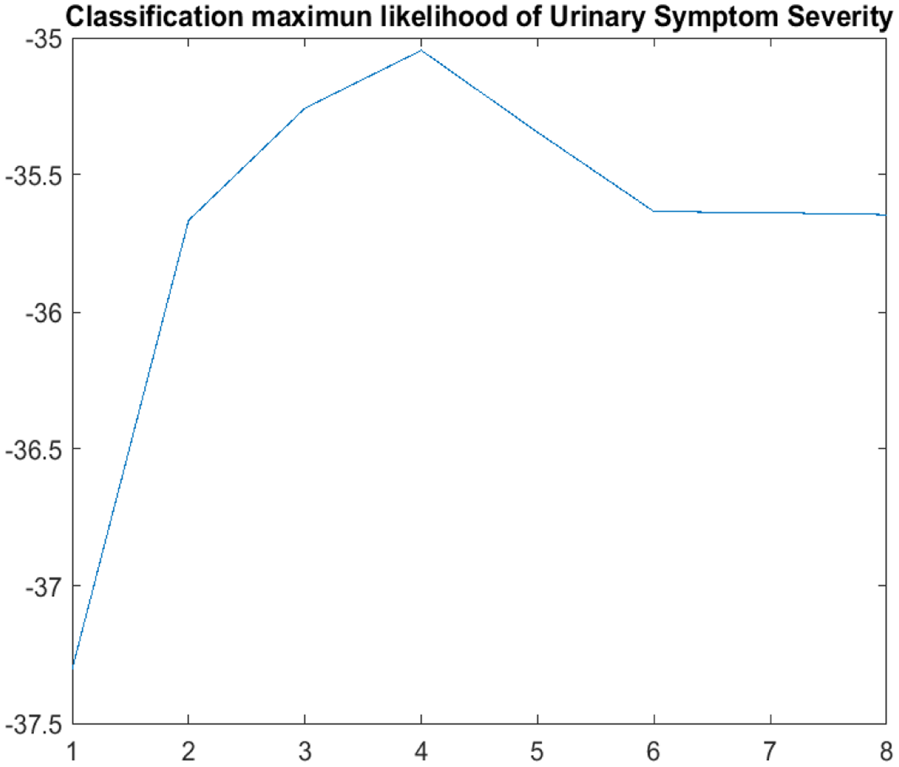
Predictive classification log-likelihood for K = 1, ⋯, 8.

As displayed previously in Figure 1, the subgroups within these 4 panels can be characterized according to their average mean USS change trajectories as 0: moderate decline (n = 68; 17.2%), 1: mild decline (n = 96; 24.3.%), 2: stable (n = 123; 31.1%) and 3: mild increase (n = 108; 27.3%). Furthermore, these 4 subgroups in Figure 1 can also be characterized as (1, 2): low variability vs (0, 3): high variability over time. The time scale in Figure 1 is re-numbered from visit= 3 (week 4) through visit= 25 (week 48), reflecting the adjustment for RTM by the exclusion of results prior to week 4. The 0: moderate decline cluster, on average, exhibits more rapid decline from visit = 3–11 (weeks 4–20), persisting in the range of −6 to −5 units of change (essentially 1-standard deviation for USS, as sd= 6.15 at week 4) throughout the remaining follow-up period. To demonstrate the ordinal trend in terms of their longitudinal changes of the four clusters, we integrate the first derivative of subject-specific trajectory over the entire followup period for each subject and show the boxplots of the integrated derivatives in Figure 2, which shows that all the subjects in cluster 0 improve substantially; those in cluster 1 improve marginally; those in cluster 2 are essentially unchanged, and those in cluster 3 are worsening over time. Furthermore, from both Figures 1 and 2, cluster 1 and 2 have significantly smaller variabilities over time than clusters 0 and 3. It is noteworthy that the flexibility of this new functional clustering algorithm to account both for differential group-average trajectories and differential within-patient variabilities are illustrated in these subgroup profile patterns.

To understand the clinical implications of these clusters, we study the associations between the cluster membership with the one-year changes of several previously identified clinically important variables (Clemens et al., 2009), namely GUPI quality of life ranging 0 – 12 with higher score indicating lower quality of life, SF-12 Physical Component Score ranging 0 – 100 with higher score is better, SF-12 Mental Component Score ranging 0–100 with higher score is better, Patient-Reported Outcomes Information System (PROMIS) Sleep Disturbance T-score ranging 8–40 with higher scores indicating greater severity of sleep disturbance, PROMIS Fatigue T-score ranging 24 – 86 with higher scores indicating greater fatigue. We first compute the one-year changes of these five variables from the baseline. We then compute the adjusted means for these changes for the four clusters, adjusting for age, gender, and the baseline values of these variables and USS scores at visit 3. The forest plot in Figure 4 shows that subjects in cluster (0) also improve in all these clinical variables except for the SF12 mental score, and there is a clear ordinal trend across the 4 clusters for all of these clinical outcomes. These results demonstrate that while these subgroups were formed using only the longitudinal trajectories of urinary severity scores, they are associated with longitudinal changes in quality of life, sleep quality and physical and mental health. By further studying what are unique in these subgroups, we may gain insights into what are contributing to improving or worsening of these patients, which may eventually lead to targeted treatments.

Figure 4:

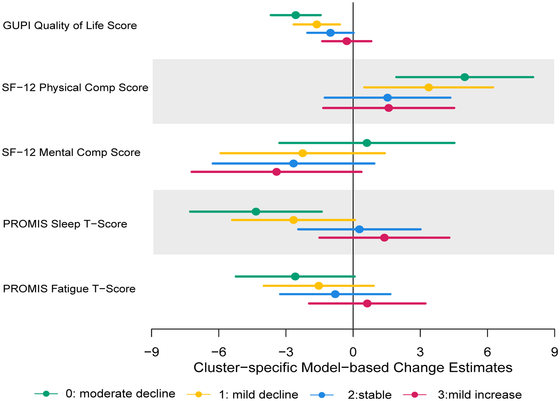
Adjusted mean changes and their 95% confidence intervals for the four clusters.

Previous attempts to identify baseline predictors of longitudinal change in UCPPS symptoms using standard methods, such as linear mixed effects models or functional mixed effects models for continuous outcomes, were not successful, due primarily to the minimal average change of continuous measures longitudinally, and the substantial differential within-patient longitudinal variability. Following those initial failures using standard mixed effects models, a preliminary version of this functional clustering approach was applied to the two primary UCPPS outcomes, and baseline clinical and psychosocial variables were evaluated as potential predictors of pelvic pain severity (PPS) change and urinary symptoms severity (USS) change (Naliboff et al., 2017). Despite producing useful functional clustering results, that earlier algorithm was computationally inefficient, sometimes failed to converge within several days of iterations, and had not yet been validated within a rigorous simulation study, as now reported here (Section 4). Furthermore, there was not an accompanying information-based criterion to suggest the optimal number K of clusters, as we have now proposed (Section 2).

Consequently, we proceeded to explore what baseline factors might be predictive of longitudinal USS change, as represented by these new functional cluster membership classifications coded 0, 1, 2, 3 as an ordinal outcome variable. By implementing ordinal logistic regression modeling for the cumulative probability of lower ordered cluster membership which means more likely to improve over time, an extensive set (number of variables = 40) of baseline factors were considered: USS score (week 4), age, sex, duration of UCPPS symptoms (< 2, 2+ yrs), and baseline measures of the RAND Interstitial Cystitis Epidemiology Study (RICE) painful filling, RICE painful urgency, 8 binary indicators of type and location of pelvic pain, PROMIS sleep T-score, Brief Pain Inventory (BPI) average pain, widespreadness of non-urologic pain, SF12 Physical Component Score (PCS), SF12 Mental Component Score (MCS), indicators for chronic overlapping pain syndromes (COPCs) including temporomandibular disorder (TMD), fibromyalgia (FMS), irritable bowel syndrome (IBS) and chronic fatigue syndrome (CFS), PROMIS fatigue T-score, PROMIS anger T-score, Hospital Anxiety and Depression Scale (HADS) depression score, HADS anxiety score, Positive and Negative Affect Schedule-Trait (PANAS) subscales, pain catastrophizing score (CSQ) and perceived stress score (PSS). Using a stepwise selection procedure, with p < 0.10 as inclusion criterion, a strict p < 0.05 as retention criterion, and forcing inclusion of baseline USS score at Week 4 as RTM- adjustment for baseline, three additional baseline predictors were identified, viz., PROMIS Sleep T-Score, RICE Painful Urgency and SF-12 PCS. Because of missing data in the covariates not included in the final model, the stepwise procedure utilized only n = 337 subjects in the analysis. We refit the final model with all the subjects (n = 374) with complete data. As shown in Table 1, after adjustment for baseline USS at week 4, lower PROMIS sleep disturbance T-score, absence of RICE painful urgency and higher levels of physical quality of life (SF-12 PCS) are each associated (p < 0.05) with a higher likelihood of patient classification into lower ordered functional clusters (decline) over the 48-week follow-up period. In contrast, our previous extensive longitudinal analyses, after adjustment for baseline USS scores, failed to identify a set of baseline predictors within a multivariable model.

Table 1:

Ordinal Logistic Regression Model Results for Relating Baseline Factors to Cumulative Probability of Lower Ordered Cluster Membership (0: moderate decline, 1: mild decline, 2: stable, 3: mild increase)(p < 0.05, n = 374)

Variable	Coefficient	Standard Error	Wald Chi-Square	p-value
Intercept (threshold 1): 0 vs (1,2,3)	−2.2541	0.9232	5.9615	0.0146
Intercept (threshold 2): (0,1) vs (2,3)	−0.8400	0.9158	0.8414	0.3590
Intercept (threshold 3): (0,1,2) vs (3)	0.6727	0.9157	0.5397	0.4625
Urinary Symptoms Severity (Week 4)	0.1729	0.0211	67.4747	< 0.0001
PROMIS Sleep disturbance T-Score	−0.0424	0.0120	12.5645	0.0004
RICE Painful Urgency (0: absent; 1: present)	−0.5937	0.2363	6.3142	0.0120
SF12 Physical Composite Score (PCS)	0.0268	0.0105	6.4592	0.0110

4. Simulation

A simulation study was conducted to evaluate the performance of proposed functional clustering approach. We compare our methods with the latent mixture model-based functional high-dimensional data clustering algorithm (FunHDDC) developed by Bouveyron and Jacques (2011), which assumed a Gaussian distribution of the principal components. Jacques and Preda (2014) reviewed most of the main existing algorithms for functional data clustering and compared correct classification rates (C-rate) for different approaches. The FunHDDC is the overall best approach according to Jacques and Preda (2014). We also compare the results with K-means as it is still widely used.

We simulated the data based on the estimates of the application in Section 3. The simulation data has four clusters which has the same sample size (68,96,123,108) as the real dataset. We generate data using y_ijk = f_k(t) + r_ik(t) + e_i, where t = {t₁, ⋯, t₂₃}, f_k(t) is the mean or population functional trajectory of the kth cluster, $e_i~N\left(0,{\sigma }_2^2\right)$. We used four cluster-average means from the Urinary Symptom Severity. The random functional deviations r_ik(t) is a draw from $N\left(0,{\sigma }_{ik}^2\Sigma (t)\right)$, where Σ = R¹(t, t), R¹(t₁, t₂) is reproducing kernel covariance that generated from Bernoulli polynomials (Gu, 2013, section 2.3.3). The Bernoulli polynomials are defined as ψ₁(t) = t − 0.5, ${\psi }_2(t)=0.5\left\{{\psi }_1^2(t)-\frac{1}{12}\right\}$ and ${\psi }_4(t)=\frac{1}{24}\left\{{\psi }_1^4(t)-\frac{1}{2}{\psi }_1^2(t)+\frac{7}{240}\right\}$. The reproducing kernel is defined as R¹(t₁, t₂) = ψ₂(t₁)ψ₂(t₂) − ψ₄(t₁ − t₂). In the first setting (Setting 2) we simulated the data using the parameters estimated from the real data where ${\sigma }_{11}^2=3738$, ${\sigma }_{12}^2=311$, ${\sigma }_{13}^2=215$, ${\sigma }_{14}^2=1900$, ${\sigma }_{21}^2=5.9$, ${\sigma }_{22}^2=2.7$, ${\sigma }_{23}^2=1.1$, ${\sigma }_{24}^2=5.3$. It can be seen from Figure 5 that the second panel is very similar to our real data. We then increase the between-group variabilities (setting 1) and measurement errors (Setting 3) to demonstrate our methods work well even for noisier data. Figure 5 shows one of the simulated datasets from three settings. For each setting, we generate 500 datasets, and compute the correct classification rates (C-rate). The boxplots of the C-rates are shown in Figure 5. The procedure for one dataset finished in about 16 minutes on a personal desktop. For all the settings, our proposed method substantially outperforms the Fun-HDDC and K-means, although the differences are less dramatic when the signal-to-noise ratios decrease. We can also see that our proposed method performs well when the between-group variabilities are different while Fun-HDDC and K-means perform substantially worse.

Figure 5:

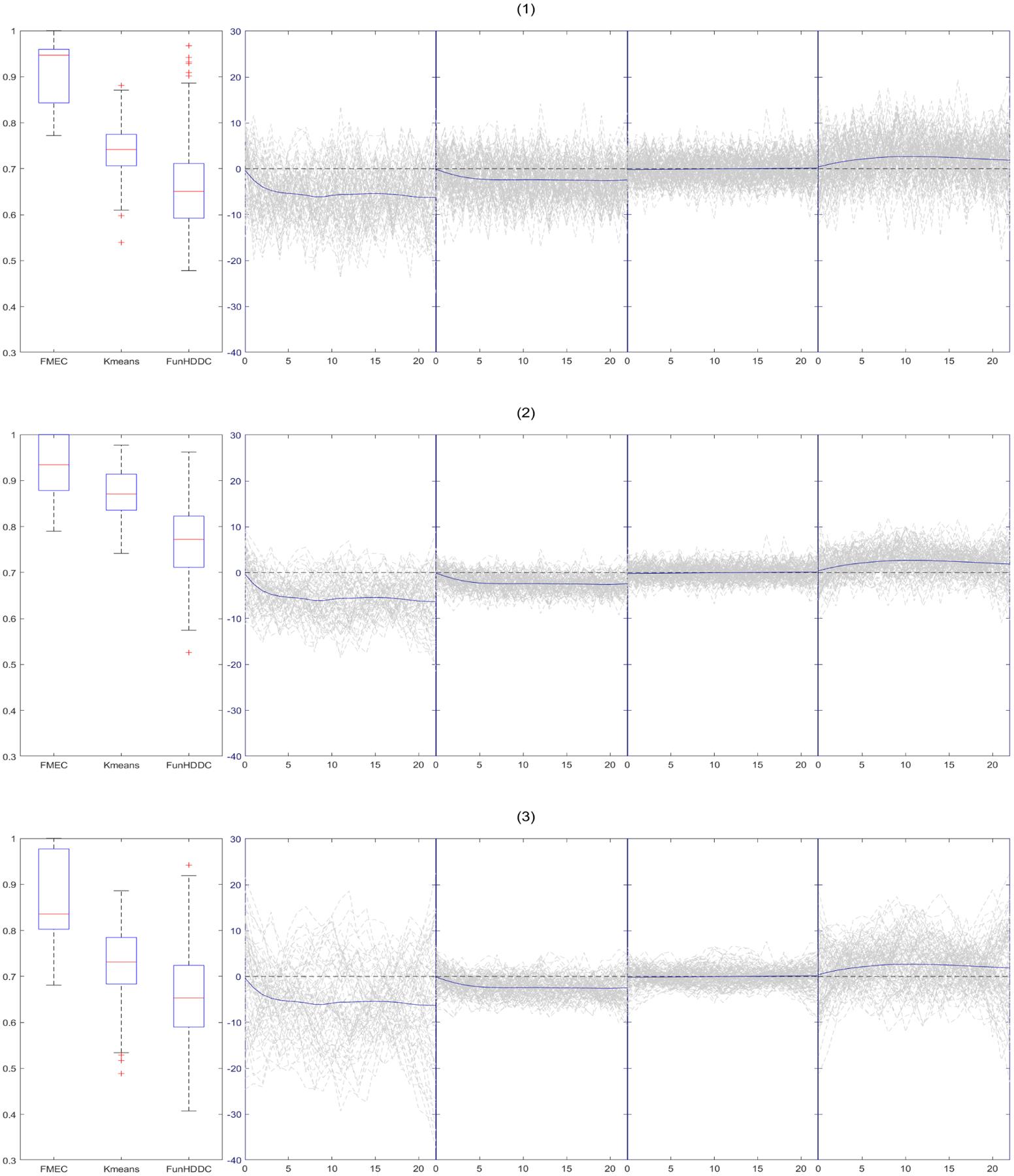
Box-plots of C-rate of 500 simulations for each settings and one simulation trajectory plots: 1) ${\sigma }_{11}^2=3738$, ${\sigma }_{12}^2=311$, ${\sigma }_{13}^2=215$, ${\sigma }_{14}^2=1900$, ${\sigma }_1^2=5.9\times 4$, ${\sigma }_2^2=2.7\times 8$, ${\sigma }_3^2=1.1\times 8$, ${\sigma }_4^2=5.3\times 4$; 2) ${\sigma }_{11}^2=3738$, ${\sigma }_{12}^2=311$, ${\sigma }_{13}^2=215$, ${\sigma }_{14}^2=1900$, ${\sigma }_1^2=5.9$, ${\sigma }_2^2=2.7$, ${\sigma }_3^2=1.1$, ${\sigma }_4^2=5.3$; 3) ${\sigma }_{11}^2=3738\times 5$, ${\sigma }_{12}^2=311\times 5$, ${\sigma }_{13}^2=215\times 5$, ${\sigma }_{14}^2=1900\times 5$, ${\sigma }_1^2=5.9$, ${\sigma }_2^2=2.7$, ${\sigma }_3^2=1.1$, ${\sigma }_4^2=5.3$.

To study the performance of the predictive classification log-likelihood methods in selecting K, we also simulated 500 datasets under the setting that mimicked the real dataset. In each of which, we applied our method with K = 2, ⋯, 7 and select the optimal K that maximizes the proposed predictive classification log-likelihood. The resultant counts are shown in Figure 6. Our method chooses the true number of clusters (K = 4) 421 (84.2%) out of 500 simulated datasets. The proposed criterion has a tendency to favor more clusters. This is a known phenomenon for other criteria such as BIC and AIC in situations without nested structures.

Figure 6:

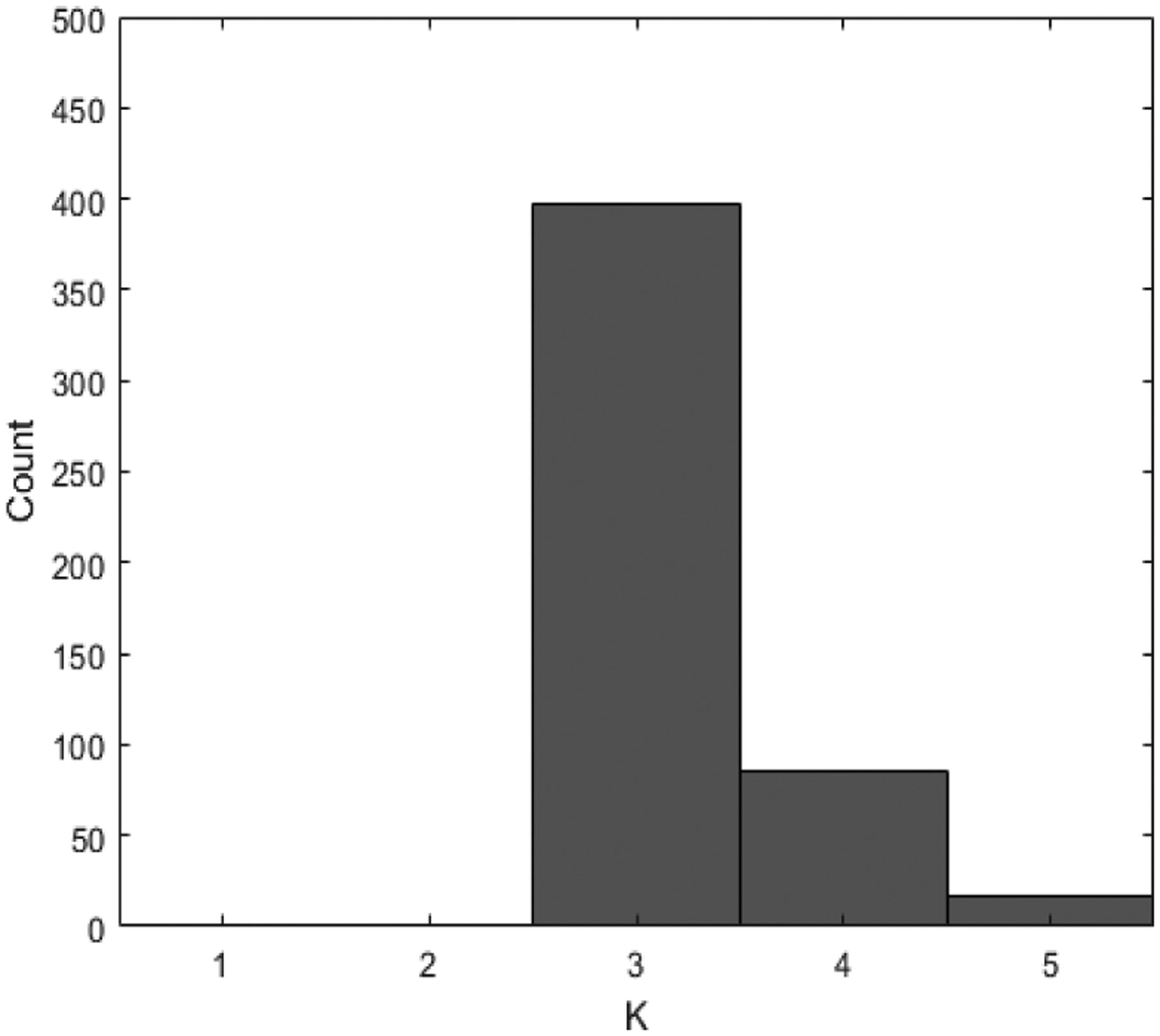
Histogram of Model selection results for setting 2.

5. Conclusion

Motivated by the complex analytical challenges of subgroup discovery based on differential longitudinal symptom profiles within the MAPP Clinical Research Network, we have proposed a functional mixed effects clustering algorithm that can take into effect nested structures in clustering functional data. The proposed method takes into account both the group-average trajectories and within-group variabilities in the functional clustering. We also proposed a cross-validation predictive classification log-likelihood criterion to select the optimal number of clusters. We applied our functional clustering method to the MAPP urinary severity longitudinal data and identified four subgroups. We found that while these subgroups were formed using only the longitudinal trajectories of urinary severity scores, they are associated with longitudinal changes of other clinically important variables previously found in UCPPS patients (Clemens et al., 2009). We further determined that after adjustment for urinary severity at week 4, lower PROMIS sleep disturbance T-score, higher levels of physical quality of life (SF-12 PCS) and absence of RICE painful urgency are each associated (p < 0.05) with higher likelihood of patient classification into improving groups over the 48-week follow-up period.

Since our discovery of subgroups in the UCPPS patients, researchers in the MAPP Research Network are actively investigating what other factors are associated with these subgroups. These additional factors include patient’s innate pain sensitivity, both brain anatomy and functional brain connectivity, immune responsiveness to bacterial antigens, and psychological influences on pain and voiding symptoms. By identifying the factors associated with a patient’s improvement or worsening, we may be able to identify different elements of pathogenesis of UCPPS, which would help us select appropriate targets for therapy.

Figure 3:

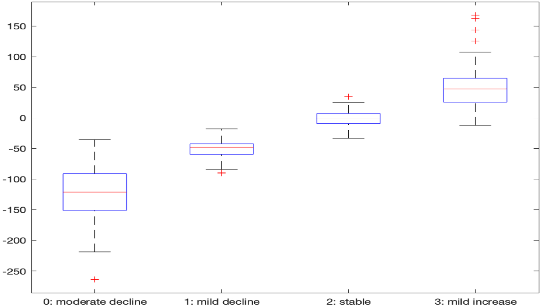
Integrated derivative of each subject over the followup period for the four clusters.

References

- Abraham C, Cornillon PA, Matzner-Løber E, and Molinari N (2003). Unsupervised curve clustering using b-splines. Scandinavian Journal of Statistics, 30(3):581–595. [Google Scholar]
- Ansley G, Kohn R, and Wong C (1993). Nonparametric spline regression with prior information. Biometrika, 80(1):75–88. [Google Scholar]
- Baudry J-P (2015). Estimation and model selection for model-based clustering with the conditional classification likelihood. Electronic journal of statistics, 9(1):1041–1077. [Google Scholar]
- Berry SH, Elliott MN, Suttorp M, Bogart LM, Stoto MA, Eggers P, Nyberg L, and Clemens JQ (2011). Prevalence of symptoms of bladder pain syndrome/interstitial cystitis among adult females in the united states. The Journal of urology, 186(2):540–544. [DOI] [PMC free article] [PubMed] [Google Scholar]
- Biernacki C, Celeux G, and Govaert G (2000). Assessing a mixture model for clustering with the integrated completed likelihood. Pattern Analysis and Machine Intelligence, IEEE Transactions on, 22(7):719–725. [Google Scholar]
- Bouveyron C and Jacques J (2011). Model-based clustering of time series in group-specific functional subspaces. Advances in Data Analysis and Classification, 5(4):281–300. [Google Scholar]
- Chiou J-M and Li P-L (2007). Functional clustering and identifying substructures of longitudinal data. Journal of the Royal Statistical Society: Series B (Statistical Methodology), 69(4):679–699. [Google Scholar]
- Ciampi A, Campbell H, Dyachenko A, Rich B, McCusker J, and Cole M (2012). Model-based clustering of longitudinal data: Application to modeling disease course and gene expression trajectories. Communications in Statistics-Simulation and Computation, 41(7):992–1005. [Google Scholar]
- Clemens J, Calhoun E, Litwin M, McNaughton-Collins M, Kusek J, Crowley E, and Landis J (2009). Validation of a modified national institutes of health chronic prostatitis symptom index to assess genitourinary pain in both men and women. Urology, 74(5):983–987. [DOI] [PMC free article] [PubMed] [Google Scholar]
- Clemens JQ, Mullins C, Kusek JW, Kirkali Z, Mayer EA, Rodríguez LV, Klumpp DJ, Schaeffer AJ, Kreder KJ, Buchwald D, Andriole G, Lucia M, Landis J, Clauw D, and Groupothers MRNS (2014). The MAPP Research Network: a novel study of urologic chronic pelvic pain syndromes. BMC urology, 14(1):1–6. [DOI] [PMC free article] [PubMed] [Google Scholar]
- Ferraty F and Vieu P (2006). Nonparametric functional data analysis : theory and practice. Springer series in statistics. Springer, New York. [Google Scholar]
- Ganesalingam S (1989). Classification and mixture approaches to clustering via maximum likelihood. Journal of the Royal Statistical Society. Series C (Applied Statistics), 38(3):455–466. [Google Scholar]
- Giacofci M, Lambert-Lacroix S, Marot G, and Picard F (2013). Wavelet-based clustering for mixed-effects functional models in high dimension. Biometrics, 69(1):31–40. [DOI] [PubMed] [Google Scholar]
- Golay X, Kollias S, Stoll G, Meier D, Valavanis A, and Boesiger P (1998). A new correlation-based fuzzy logic clustering algorithm for fmri. Magnetic Resonance in Medicine, 40(2):249–260. [DOI] [PubMed] [Google Scholar]
- Greven S and Kneib T (2010). On the behaviour of marginal and conditional aic in linear mixed models. Biometrika, 97(4):773–789. [Google Scholar]
- Griffith JW, Stephens-Shields AJ, Hou X, Naliboff BD, Pontari M, Edwards TC, Williams DA, Clemens JQ, Afari N, Tu F, Lloyd R, Patrick D, Mullins C, Kusek J, Sutcliffe S, Hong B, Lai H, Krieger J, Bradley C, Kim J, and Landis J (2016). Pain and urinary symptoms should not be combined into a single score: psychometric findings from the MAPP Research Network. The Journal of urology, 195(4 Part 1):949–954. [DOI] [PMC free article] [PubMed] [Google Scholar]
- Gu C (2013). Smoothing spline ANOVA models, volume 297. Springer Science & Business Media. [Google Scholar]
- Guo W (2002). Functional mixed effects models. Biometrics, 58(1):121–128. [DOI] [PubMed] [Google Scholar]
- Heard NA, Holmes CC, and Stephens DA (2006). A quantitative study of gene regulation involved in the immune response of anopheline mosquitoes: An application of bayesian hierarchical clustering of curves. Journal of the American Statistical Association, 101(473):18–29. [Google Scholar]
- Held P, Hanno P, Wein A, MV P, and MA C (1990). Epidemiology of Interstitial Cystitis. In Interstitial Cystitis. London: Springer Verlag. [Google Scholar]
- Ieva F, Paganoni AM, Pigoli D, and Vitelli V (2013). Multivariate functional clustering for the morphological analysis of electrocardiograph curves. Journal of the Royal Statistical Society: Series C (Applied Statistics), 62(3):401–418. [Google Scholar]
- Jacques J and Preda C (2013). Funclust: A curves clustering method using functional random variables density approximation. Neurocomputing, 112:164–171. [Google Scholar]
- Jacques J and Preda C (2014). Functional data clustering: a survey. Advances in Data Analysis and Classification, 8(3):231–255. [Google Scholar]
- James GM and Sugar CA (2003). Clustering for sparsely sampled functional data. Journal of the American Statistical Association, 98(462):397–408. [Google Scholar]
- Kayano M, Dozono K, and Konishi S (2010). Functional cluster analysis via orthonormalized gaussian basis expansions and its application. Journal of Classification, 27(2):211–230. [Google Scholar]
- Kullback S and Leibler RA (1951). On information and sufficiency. The annals of mathematical statistics, 22(1):79–86. [Google Scholar]
- Landis JR, Williams DA, Lucia MS, Clauw DJ, Naliboff BD, Robinson NA, van Bokhoven A, Sutcliffe S, Schaeffer AJ, Rodriguez LV, et al. (2014). The MAPP Research Network: design, patient characterization and operations. BMC urology, 14(1):58. [DOI] [PMC free article] [PubMed] [Google Scholar]
- Liang H, Wu H, and Zou G (2008). A note on conditional aic for linear mixed-effects models. Biometrika, 95(3):773–778. [DOI] [PMC free article] [PubMed] [Google Scholar]
- Luan Y and Li H (2003). Clustering of time-course gene expression data using a mixed-effects model with b-splines. Bioinformatics, 19(4):474–482. [DOI] [PubMed] [Google Scholar]
- McNicholas PD and Murphy TB (2010). Model-based clustering of longitudinal data. Canadian Journal of Statistics, 38(1):153–168. [Google Scholar]
- Naliboff B, Stephens A, Lai H, Griffith J, Clemens J, Lutgendorf S, Rodriguez L, Newcomb C, Sutcliffe S, Guo W, Kusek J, and Landis J (2017). Clinical and psychological predictors of urologic chronic pain symptom change over one year: A prospective study from the MAPP Research Network. The Journal of urology, 198(4):848–857. [DOI] [PMC free article] [PubMed] [Google Scholar]
- Peng J and Muller H-G (2008). Distance-based clustering of sparsely observed stochastic processes, with applications to online auctions. The Annals of Applied Statistics, 2(3):1056–1077. [Google Scholar]
- Pontari M (2013). Etiology of chronic prostatitis and chronic pelvic pain syndrome: psychoimmunoneurendocrine dysfunction (pine syndrome) or just a really bad infection? World Journal of Urology, 31:725–731. [DOI] [PubMed] [Google Scholar]
- Propert K, McNaughton-Collins M, Leiby B, O’Leary M, Kusek J, Litwin M, and Network CPCR (2006). A prospective study of symptoms and quality of life in men with chronic prostatitis/chronic pelvic pain syndrome: the national institutes of health chronic prostatitis cohort study. The Journal of urology, 175:619–625. [DOI] [PubMed] [Google Scholar]
- Qin L (2004). Functional models using smoothing splines, a state space approach. Dissertation. University of Pennsylvania. [Google Scholar]
- Qin L and Guo W (2006). Functional mixed-effects model for periodic data. Biostatistics, 7(2):225–234. [DOI] [PubMed] [Google Scholar]
- Ray S and Mallick B (2006). Functional clustering by bayesian wavelet methods. Journal of the Royal Statistical Society: Series B (Statistical Methodology), 68(2):305–332. [DOI] [PMC free article] [PubMed] [Google Scholar]
- Stephens-Shields AJ, Clemens JQ, Jemielita T, Farrar J, Sutcliffe S, Hou X, Landis JR, et al. (2016). Symptom variability and early symptom regression in the MAPP study, a prospective study of urologic chronic pelvic pain syndrome. The Journal of urology, 196(5):145–1455. [DOI] [PMC free article] [PubMed] [Google Scholar]
- Suskind A, Berry S, Ewing B, Elliott M, Suttorp M, and Clemens J (2013). The prevalence and overlap of interstitial cystitis/bladder pain syndrome and chronic prostatitis/chronic pelvic pain syndrome in men: results of the rand interstitial cystitis epidemiology male study. The Journal of urology, 189(1):141–145. [DOI] [PMC free article] [PubMed] [Google Scholar]
- Tokushige S, Yadohisa H, and Inada K (2007). Crisp and fuzzy k-means clustering algorithms for multivariate functional data. Computational Statistics, 22(1):1–16. [Google Scholar]
- Vaida F and Blanchard S (2005). Conditional akaike information for mixed-effects models. Biometrika, 92(2):351–370. [Google Scholar]
- Wecker W and Ansley C (1983). The signal extraction approach to nonlinear regression and spline smoothing. Journal of the American Statistical Association, 78:81–89. [Google Scholar]