External hardware and sensors, for improved MRI

Abstract

Complex engineered systems are often equipped with suites of sensors and ancillary devices that monitor their performance and maintenance needs. MRI scanners are no different in this regard. Some of the ancillary devices available to support MRI equipment, the ones of particular interest here, have the distinction of actually participating in the image acquisition process itself. Most commonly, such devices are used to monitor physiological motion or variations in the scanner’s imaging fields, allowing the imaging and/or reconstruction process to adapt as imaging conditions change. ‘Classic’ examples include electrocardiography (ECG) leads and respiratory bellows to monitor cardiac and respiratory motion, which have been standard equipment in scan rooms since the early days of MRI. Since then, many additional sensors and devices have been proposed to support MRI acquisitions. The main physical properties that they measure may be primarily ‘mechanical’ (e.g., acceleration, speed, torque), ‘acoustic’ (sound, ultrasound), ‘optical’ (light, infrared) or ‘electromagnetic’ in nature. A review of these ancillary devices, as currently available in clinical and research settings, is presented here. In our opinion, these devices are not in competition with each other: as long as they provide useful and unique information, do not interfere with each other and are not prohibitively cumbersome to use, they might find their proper place in future suites of sensors. In time, MRI acquisitions will likely include a plurality of complementary signals. A little like the microbiome that provides genetic diversity to organisms, these devices can provide signal diversity to MRI acquisitions and enrich measurements. Machine-learning (ML) algorithms are well suited at combining diverse input signals toward coherent outputs, and they could make use of all such information toward improved MRI capabilities.

Introduction

Complex modern engineering creations are commonly equipped with suites of sensors that sample physical parameters such as temperature, luminosity, torque, or acceleration. Such information can be used to help improve the safety, performance and/or durability of the overall assembly. Similarly, MRI scanners are equipped with ancillary hardware that keeps track of their performance and maintenance requirements, for example by measuring helium filling, temperature, or reflected RF power. But sensors can also be part of the image acquisition process itself, as described here.

While classic devices such as respiratory bellows and electrocardiography (ECG) leads have been available since the early days of MRI, other devices have been introduced more recently. These sensors may monitor physiological motion or electromagnetic fields, allowing the MRI acquisition and/or reconstruction process to adapt to non-ideal situations as they occur to alleviate their impact on image quality. In the present paper, we review the various types of sensors currently available to supplement MRI acquisitions in clinical practice and/or research settings. These sensors are grouped below according to the main physical properties they measure, which may be primarily ‘mechanical’ (e.g., acceleration, speed, torque), ‘acoustic’ (sound and ultrasound), ‘optical’ (light, infrared) or ‘electromagnetic’ in nature. ‘Classic devices’, which have been staples of MRI suites for a long time, are presented separately. But first, we will review the various ways that sensor signals, irrespective of sensor type, may be employed to influence the MRI acquisition and reconstruction process.

Materials and Methods

A. How sensor information gets used

A.1. Background

MRI pulse sequences may run their course in pre-determined fashion, or adapt in real-time to developing situations. The latter case is typically referred to as a ‘prospective’ acquisition, whereby information from sensors and/or from the MRI signals guide real-time decisions such as what k-space locations should be sampled next, and/or where the imaging plane/volume should be moved to. Sensor-based information can also be recorded and employed retrospectively, at the image reconstruction stage, to help improve image quality. Most of the sensors/devices discussed here provide information about patient motion.

People move faster than an MRI scanner measures images, be this gross motion, breathing or the beating heart. Motion artifacts remain a major problem in clinical MRI: in neuro MRI, for example, motion may cause 2 to 4% of scans to be non-diagnostic (1,2). For all applications combined, nearly 20% of MRI exams were reported to include scan(s) repeated due to motion (3). These numbers suggest there might be considerable economic value in hardware and external sensors that could help better capture, resolve and/or compensate for patient motion. The text below will differentiate between cyclic motion, such as breathing and heartbeats, and random events such as gross motion. In general, artifacts can be suppressed effectively if the underlying motion is known with sufficient precision and accuracy (4–6). External devices that function independently from the MRI scanner have the advantage that they do not affect the MRI contrast, do not take time away from the MRI acquisition, and may prove easier to implement. Besides motion compensation, other devices may be geared toward monitoring scanner-related rather than patient-related parameters, for example the performance of the imaging gradients. The information they provide can be used retrospectively, to improve image quality.

A.2. Cyclic motion – triggering and binning

Cyclic motion can typically be handled even if it involves elaborate organ deformations, and even if sensor signals only capture the motion indirectly and/or qualitatively. For example, respiration or cardiac cycles can be monitored using 1D signals from respiratory cushions and belts (7,8) or ECG leads (9,10). This information can be used prospectively to trigger the MRI acquisition, or retrospectively to create images at one or more specific phase(s) of the cyclic motion (Fig. 1a) (9). When several phases are reconstructed, the resulting images can capture the underlying motion, typically the respiratory cycle and/or the beating motion of the heart (11,12). Triggers may also be provided by the volunteer her/himself, in voluntary fashion, as sometimes done in functional MRI (fMRI) using handheld devices with button(s)/lever(s) (13); in this case, the temporal changes to be resolved are associated with brain function, as opposed to physiological motion.

Fig. 1:

a) Acquisition periods in prospective triggering and retrospective gating of cardiac data. b) Visualization of the six degrees of freedom which are used for rigid body motion correction (3x translation, 3x rotation). c) Severe banding artifacts caused by spin-history effects that can be largely suppressed when using prospective motion correction. d) Principles of prospective and retrospective motion correction when using an external motion tracking device.

A.3. Random motion events – prospective correction

When the imaged anatomy gets displaced/rotated due to gross patient motion, the position and orientation of the imaging plane/volume can be changed in real time to track it (4,14–16). Such real-time tracking works best when the imaged anatomy undergoes ‘rigid-body’ motion, which can be described with three parameters for translation and another three for rotation, for a total of six degrees-of-freedom (6DOF), see Fig. 1b. The sensor(s) must provide quantitative information about six of these DOFs, to track the anatomy as it moves. Because the head is a prime example of a ‘rigid body’, such real-time adaptive motion-compensation schemes are most often encountered in neuro applications. Besides correction of gross motion, prospective motion correction can greatly reduce so-called spin-history effects whereby different spatial locations in the anatomy see different histories of spin excitations and magnetization relaxation (17), see Fig. 1c. In general, motion information can be used beyond the correction of image data. For example, in diffusion MRI one can use motion information to preserve the alignment of subject anatomy and diffusion gradient orientation (18). Sensor information can also be used to detect which data/images are most likely to be corrupted by motion so they can be reacquired (19–21), at the cost of prolonged scan times.

Requirements on tracking accuracy tend to be relatively high: for example, Maclaren et al (22) concluded that precision should be below 1/5 of the voxel size. While having accurate/precise motion estimates is important, having them quickly and often is also key, especially in the presence of fast motion. Time delays in generating motion estimates is typically referred to as the ‘latency’, and how often these estimates are generated as their ‘frequency’. Unlike image-based solutions, where motion updates are available only when a new image is acquired (17), external devices may achieve much higher frequency (15). Methods have been developed to feed motion information back to scanners, to alter the position/orientation of imaging planes/volumes (23–26).

A.4. Retrospective corrections

A considerable advantage of retrospective corrections is that they do not need to be causal, i.e., both past and future information can be employed when handling any given time point. For example, requirements on tracking precision might be relaxed by as much as 5- or 10-fold as filters involving both past and future motion estimates may help obtain cleaner estimates (27). Retrospective methods (Fig. 1d) may apply to cyclic motion and/or random motion events. Especially in the presence of large motion, these methods tend to work better in 3D imaging as the imaged anatomy may remain within the imaged volume at all times, as opposed to 2D imaging where the anatomy might wander outside the slice leading to irrecoverable losses of information. Provided that sensor signals are quantitative, well synchronized with the MR acquisition and have sufficient information content, k-space data can be manipulated at the reconstruction stage to account for translations, rotations and even non-rigid deformations (5). Given that motion estimates are obtained with sufficient frequency, motion correction can be applied at the level of individual k-space readout (28); however, when handling rotations, motion-based alterations to the k-space data may lead to k-space regions being undersampled, which in turn may lead to image artifacts.

Beyond the reconstruction of MRI images, motion information can also take its place within more elaborate algorithms, for example in fMRI postprocessing (29). Beyond motion, other relevant parameters such as measurements of MRI-related fields can also be utilized during the image reconstruction process.

A.5. Clocks, reference systems, and scaling

While external devices add relevant information to the image acquisition scheme, they operate mostly independently from the MRI system, making synchronization a possibly difficult task. In prospective applications, ‘synchronization’ may become synonymous with ‘low latency’, meaning that ‘now’ should have essentially the same meaning for all devices. In contrast, in retrospective applications, synchronization may take the form of a common clock that places time tags on incoming data of all types. The community has been active in providing hardware solutions to synchronization issues (30), as well as standardized formats and interfaces (31,32).

In addition to common clocks, common axes may also be needed. Ideally, a transformation matrix may be found between the scanner coordinate system and the coordinate system that most naturally describes the sensor data (4,33). The accuracy of such transformation may play a key role in determining the quality of the overall motion correction process (34).

Furthermore, proper scaling/conversion may be needed to convert raw sensor signals into quantitative motion estimates. To do so, separate calibration test(s) may be required. For some of the devices presented here, no such calibration steps could be devised; as such, these devices can provide an observation of change but not quantify they underlying motion. Such qualitative waveforms will typically be used to enable gating/triggering strategies (above), allowing images to be reconstructed at specific phases of a cyclic motion.

A.6. Particular challenges

Motion types that are non-repetitive and non-rigid, for example peristalsis, tend to be the most difficult to handle. But even for simpler motion types, such as that of a head, interactions between the moving anatomy and the scanner’s fields can affect MRI signals in ways that are difficult to model and account for. For example, even in a perfect scenario where motion would be accurately measured and instantaneously adapted by the system, changes in the position of the subject inside the MRI scanner will inevitably affect the coil loading, the coil sensitivity, and the B0 field through susceptibility effects (35,36).

B. ‘Classic’ devices

B.1. Respiratory bellows, pulse oximeters and ECG leads – Strengths and limitations

Ever since the early days of MRI, imaging suites have been equipped with respiratory bellows, pulse oximeters and ECG leads. Respiratory bellows generate breathing waveforms that enable respiratory gating and/or binning (section A). They are stretchable devices that wrap around the torso; as the patient breathes, their torso inflates/deflates causing the bellows to expand/contract. These changes in the length of the bellows are converted into changes in the voltage output, creating a voltage waveform that clearly captures the patient’s breathing pattern. However, bellows involve much fabric and Velcro liable to move in various ways, making them difficult to use and uncomfortable to be in. Their signals only indirectly and qualitatively capture breathing motion, in oversimplified fashion. For all of these reasons, respiratory bellows have largely fallen out of favor over the years.

Using either a pulse oximeter or an ECG system, a cardiac waveform can be obtained that enables cardiac gating/triggering (section A). Pulse oximeters are easy to use, as they simply clip onto a finger to detect heartbeat-related changes in the blood content/oxygenation of the underlying tissues. However, there is a patient-dependent delay between the moment the heart contracts and the moment that an influx of blood arrives to the finger. Furthermore, the increase in oxygenation tends to be a somewhat broad peak in time, as opposed to a sharp event. For both of these reasons, the time delay and the lack of a sharp event to trigger on, pulse oximeters may lead to cardiac images that do not precisely represent given cardiac phases, and where some unresolved cardiac motion may manifest as blurring.

In contrast, ECG signals come directly from the heart muscle (minimal delay) and provide sharp peaks for triggering purposes (usually, the R wave). However, properly installing/removing ECG leads requires some time and some degree of expertise and there is always a finite risk of confusing MRI compatible vs. non-compatible leads, potentially leading to skin burns. At a technical level, an important limitation of ECG leads in MRI comes from the magnetohydrodynamic effect (37), as positive and negative ions in blood get physically separated to some degree as blood flows through the B₀ field. Electric fields caused by the magnetohydrodynamic effect increase with B₀, making ECG leads mostly unusable at high field. As a rule of thumbs, at 1.5 T or below ECG leads tend to work very well, at 3 T they were made to work in a mostly-reliable fashion at 3T through considerable ingenuity and advanced vector-based algorithms, while at 7 T they may require considerable operator expertise and effort.

As explained in the following sections, devices based on mechanical, acoustic, optical and/or electromagnetic principles have been developed to complete or improve upon the classic devices presented here. These newer devices may be aimed at different types of motion (e.g., gross patient motion), at monitoring breathing/cardiac motion more thoroughly, quantitatively, conveniently and/or at higher B₀ fields than the classic devices described here.

C. Mechanical/inertial sensors

C.1. Background

The advent of smartphones, that can aid navigation and have features like screen tilt detection, has driven down the cost of inertial sensors in the form of micro-electromechanical systems (MEMS). MEMS sensors are built using a combination of semiconductor manufacturing techniques and micro machining to enable the construction of tiny mechanical structures as part of an integrated circuit (IC) (38). Inertial sensors rely on detecting the forces acting on a mass. This mass is suspended using a mechanical structure so that it is partially or completely decoupled from the sensor frame. The motion of the mass/inertia relative to the frame can be used to detect the acceleration and/or angular rate of the frame.

C.2. Acceleration

A vehicle is an example of an accelerating frame of reference. The passenger experiences forces from objects fixed to the vehicle - the seat - that keep them stationary with respect to the vehicle. By measuring the force that the seat exerts on their body, one can determine the acceleration of the vehicle. Accelerometers achieve this by suspending a proof mass using a flexure (directional spring) and then detecting the displacement of the mass (Fig. 2a). The larger the displacement, the larger the force the flexure is applying to the mass to keep it moving with the sensor frame. The ratio of the force over the mass is the acceleration. More pliant flexures, and/or heavier masses, would lead to greater relative displacements between mass and frame and to more precise measurements. But on the other hand, the mechanical resonance frequency of such system, which is proportional to the square root of the flexure stiffness over the mass, would be lower, leading to a more limited usable bandwidth for the sensor. This tradeoff between sensitivity and bandwidth must be considered when selecting an accelerometer for MRI applications, as the mechanical resonances of the scanner are of a similar order of magnitude as those of some commercially available accelerometers. Optical accelerometers have also been proposed (39), however their availability is still limited.

Fig. 2:

a) The inertia of the proof mass results in a deformation of the flexure proportional to the acceleration of the frame. b) A mass is driven (left-right) using an actuator. When the sensor frame rotates the mass begins to oscillate in the vertical axis with an amplitude proportional to the angular rate. c) An example variable capacitor used to sense displacement of the proof mass in MEMS inertial sensors.

In MR motion detection the range of accelerations are typically quite small, less than one g, where g is the apparent acceleration caused by the Earth’s gravitational field. Gravitation is a “real” force acting on the proof mass, and it can therefore be measured even when no acceleration is present. The ability to detect the direction of the Earth’s gravitational field is particularly helpful in MR applications because - as with many construction projects - a gravity level is used to align the x, y and z gradient coils during the scanner installation. The gravity vector would therefore, typically, align closely with one of the principal gradient axes that define the imaging coordinate system. As a result, measuring the direction of the gravitation field provides useful information about the orientation of the sensor relative to the gradient coils.

C.3. Angular rate

For measuring the angular rate, one can first consider a Foucault pendulum as an example. The coordinate frame of an observer on Earth watching the pendulum is rotating with the planet; as a result, the pendulum path as observed from above appears to rotate. From the observer’s viewpoint, this deviation in the bob’s path can be interpreted as proof that she/he is in a rotating frame of reference. Because the Earth turns at a constant angular rate, Foucault’s pendulum also rotates at a constant rate (equal to ${15}^o\times \sin \left(latitude\right)$ degrees/hour), but more generally, in a system where the angular rate might keep changing, one could keep monitoring the pendulum to dynamically evaluate these changes. It is important to note that the mass needs to be moving for the deviation to be observed (Fig. 2b), and that it is the rate of change in the orientation of the sensor frame that is being measured, a quantity that can take on values much beyond that of the Earth’s angular rate of change.

C.4. Measurement considerations

When using rate sensors to track the orientation or position of an object it is important to consider the integration steps. In the case of an accelerometer, converting acceleration into displacement requires two integration steps: the first to obtain velocity, and then another to obtain displacement. Each acceleration measurement has some uncertainty, and as such, the variance in estimating velocity increases proportionally with the number of samples being integrated. After a second integration, the variance scales to the third power of the integration period, meaning that displacement values may become increasingly unreliable with time. In addition to this drift, the orientation of the accelerometer frame at each instant is required for correct interpretation of the acceleration vector. Accelerometers are therefore best suited as complements to displacement measurement techniques that can track these drifts over short periods. The combination of an angular rate sensor and an accelerometer represents a good example of sensor fusion, whereby the direction of the gravity vector, measured by the accelerometer, is used to track the drift caused by noise and biases that accumulate when integrating the angular rate sensor (40). For gating applications where quantitative measurements are not necessary, rate sensors are particularly sensitive to small impulses and can be used for cardiac and respiratory gating (41).

When using MEMS devices in an MR scanner it is important to consider how the displacement of the proof mass is sensed. Perhaps the most widespread method is by building overlapping combs between the proof mass and the frame to form a variable capacitor, where the change in capacitance is proportional to the displacement of the mass (Fig. 2c). While sensing displacements using electric fields is compatible with MRI, the mass will carry an electrical charge. In the case of an angular rate sensor the proof mass is oscillating (Fig. 2b), resulting in a Lorentz force that will bias the angular rate measurement. This additional bias is dependent on the orientation of the rate sensor and would need to be tracked using some form of sensor fusion algorithm.

D. Acoustic devices – sound and ultrasound

D.1. Background

Sounds from the human body often have considerable diagnostic value, and as such, it may not be surprising that the typical, almost caricatural representation of a physician is someone with a stethoscope around her/his neck. While auscultation has been used for time immemorial, the stethoscope itself was first invented only in 1816 by a French physician, Dr. René Laennec, as a way to avoid the awkwardness of having to place his ear directly in contact with patients (42). Auscultation may involve more than just passive listening, as the physician can further use percussion to create sounds through small impacts. Similarly, some of the devices considered below both create sound/ultrasound disturbances as well as record the tissues’ response to these disturbances.

Unlike electromagnetic waves, and waves on a pond, which are both examples of ‘transverse waves’, pressure waves such as sound and ultrasound are ‘longitudinal waves’. This is because the oscillatory motion of the molecules in the medium produced by pressure waves occurs along the same direction that the wave propagates in. The motion of the molecules creates areas of compression (higher density and relative pressure) and areas of rarefaction (lower density and relative pressure). These spatial variations in pressure further vary in time as the wave propagates.

Pressure waves, like all waves, are described by their wavelength, λ, their period, τ, their frequency, f, and their speed, c. The wavelength is the distance between consecutive pressure peaks, the period is the time delay between two consecutive pressure peaks passing through a same point, the frequency is the inverse of the period, and the speed is given by:

$$c=f\times \lambda .$$ [1]

The speed of a pressure wave depends only on the medium it propagates in, not on the device that creates it: for example, the speed of sound is about 330 m/s in air and 1540 m/s in biological soft tissues (43). In contrast, the frequency of a pressure wave depends only on the device that creates it, not on the medium that it propagates in. Meanwhile, λ can be thought of as the flexible parameter that will take whichever value is needed for Eq. 1 to be fulfilled.

D.2. Elastography, digital stethoscopes

Perhaps not surprisingly, large collections of molecules bound by electric forces will bounce and shake in a three-dimensional manner when hit with a mechanical disturbance. The generation and propagation of pressure waves, as described above, represent one way for energy to be channeled in, but it is not the only one. Much-slower shear waves involve particle motion in a direction perpendicular to the direction of wave propagation; the speed and phase of shear waves, and how these vary with frequency, can reveal much about the elastic properties of the tissues they traverse (44). Shear Wave Elastography (SWE) is a technique that involves generating and characterizing shear waves in materials and tissues. MR Elastography (MRE) (45) is a particular example of SWE that uses vibrational actuators, typically operating at about 50 or 60 Hz, pressed against tissues to ‘shake’ them. Not unlike what is done in respiratory or cardiac gating, triggers are sent to the scanner to keep the MRI acquisition ‘in sync’ with this actuator-induced motion. In this case, rapid motion can be resolved by MRI thanks to the measurable and reliably periodic nature of this motion.

While actuators create mechanical disturbances and do not receive signals, in contrast electronic stethoscopes only receive signals and do not create disturbances. These devices are very similar to conventional stethoscopes except that the ‘listening’ is done by electronic components that digitize the incoming sounds. Digital stethoscopes have been used to monitor patients during MRI (46) and to provide triggers for cardiac MRI (47,48). Sound-based cardiac triggers are especially useful at high field, where ECG signals prove unreliable due to magnetohydrodynamic effects (37). Careful processing may be required, however, to discriminate faint cardiac-related sounds from the background cacophony of an MRI scanner in action.

D.3. Ultrasound scanners and sensors

Modern ultrasound transducers typically consist of a linear arrangement of separate piezoelectric elements, often made of lead zirconate titanate (PZT) crystals. While a linear arrangement enables 2D imaging, crystals may be arrayed in a 2D matrix instead to enable 3D imaging. Acquisition rates of 20 frames per second (fps) or more, which are difficult to achieve with MRI, are common in ultrasound imaging. As MRI offers superior tissue contrasts and ultrasound imaging offers superior temporal resolution, hybrid approaches combining both of these strengths have been sought. To this end, hardware components associated with both imaging modalities need to be combined. While the piezoelectric crystals themselves tend to be readily MRI-compatible, their associated electronics, wirings and frames, in the probe head, may not be. Anecdotally, older ultrasound probes, which tend to have simpler designs and less processing power directly in the probe head, may often prove more readily MR-compatible than newer ones.

Starting in the early 2000’s (49), a few different groups successfully brought various commercial ultrasound probes within the MRI environment, for hybrid MRI-ultrasound acquisitions (50–53). More recently, a remarkable MR-compatible 3D-imaging probe was developed at the University of Wisconsin and General Electric (54). Ultrasound (B-mode) images, whether 2D or 3D, can be used to resolve and characterize breathing motion (49–51,54), and Doppler imaging can help detect the beating motion of the heart for MRI triggering purposes (52). In all of these experiments, the actual probe was brought inside the MRI scan room while the ultrasound scanner itself was kept safely away, connected to the probe by extra-long cables. In contrast, an impressive MR-compatible ultrasound scanner was built at Fraunhofer MEVIS together with Fraunhofer IBMT (55) that can be rolled right next to an MRI scanner: in this case, not only the probe but the entire scanner can be brought within the MRI environment (Fig. 3a).

Fig. 3:

a) An ultrasound scanner developed at Fraunhofer MEVIS can be rolled right next to an MRI scanner (image from (55)). b) MR-compatible ultrasound-based sensors can be placed on the abdomen and/or chest. c) Example signals from such sensors are shown (sensor placed on the abdomen, during free breathing).

The usefulness of ultrasound imaging, as a modality, comes to a large degree from the training and the experienced hand of the technologist holding the probe; however, such a hand is generally unavailable within the confines of an MRI bore. Typical solutions to this problem have involved mechanical devices that can hold and press the probe against the skin, and/or imaging probes that are flat in shape and thus can be held in place against the body, for example using bands of fabric. Alternatively, small ultrasound sensors were developed that can easily attach/detach onto/from the skin (56), Fig. 3b–c. Even though signals from such sensors cannot be reconstructed into images, they can still detect internal motion with high temporal resolution (56–58). They can therefore act as a supplement to other imaging modalities such as MRI or PET (59). Compared to full-blown ultrasound scanners, these ultrasound sensors trade imaging functionality for greater ease-of-use, as they are small, easy to apply to the skin and can even be made wireless (60).

Overall, pressure waves and ultrasound devices can be used in a complementary fashion with MRI. These devices are well suited to monitoring physiological motion, mostly because of the high temporal resolution of their signals. In the future, the intrinsic tissue contrast of ultrasound devices, which is different from that of MRI, might be better exploited as part of the image reconstruction process, to help improve contrast and better characterize tissues.

E. Optical

E.1. Background

Patient motion can be monitored using cameras that operate in the visible and/or infrared range of the optical spectrum (4,61). Even though cameras can only sense the surface of objects, they can track the movement of rigid bodies such as the head. Applying ‘markers’ of known designs and patterns onto the skin may ease the image interpretation step, where images are converted into quantitative motion measurements. Markers are typically fixed to rigid parts of the body, such as bones or teeth, with possible impact on patient comfort and imaging workflow. The use of multiple cameras, for ‘stereoscopic’ vision, simplifies the mathematical problem of ‘depth restoration’ but also requires additional optical paths, which often prove a rare commodity within the confines of an MRI bore. In addition to rigid body motion, changes in the outline of the thorax can be employed as a surrogate for breathing, and the timing of heartbeats can be assessed through changes in surface temperature caused by an influx of blood, as detected in the red and/or infrared frequency range.

E.2. Detecting rigid-body motion

Motion of the head can be approximated using the rigid-body model, whereby the spatial location of the object is completely defined by a combination of position and orientation, referred to as a ‘pose’ in computer vision. Optical tracking is an established technology, and a range of different optical tracking approaches compatible with MRI are described below.

Stereoscopic motion tracking mimics the visual perception of the 3D world by human eyes, and typically involves two or more cameras delivering independent views of the scene. The use of on-axis lighting and retro-reflecting spheres or other high-contrast optical markers enables fast automated detection of landmarks and assignment of correspondence between images. 3D positions of every landmark are determined independently through the intersection of rays from multiple viewpoints. To track orientation, the positions of three or more landmarks on a rigid body are combined and fitted to a corresponding model. The ‘structured light method’ is a variation of the stereovision approach, where one of the cameras is replaced by a projector that displays landmarks onto the surface of the object being tracked.

3D tracking with a single camera is also feasible if the 3D geometry of the marker is precisely known and provides sufficient information based on the detectable landmarks. When a landmark is located in a camera image it provides two pieces of data: its X and Y coordinates on the camera sensor chip. As the pose of a rigid marker with several landmarks provides at least 6 DOF, from 3 or more landmarks, the 6DOF pose of the marker relative to the camera may in principle be determined. The accuracy of the determination depends on the imaging geometry, with low accuracy arising when large rotations produce only a small apparent shift of the landmarks in the image. The sensitivity of the method is improved when the marker is located close to the camera and the camera uses wide-angle optics.

E.3. Marker-based vs. markerless, and sources of errors

Optical markers of known design and pattern can be mounted externally, e.g., on the subject’s face. In markerless methods the surface of the face itself, typically a small patch close to the nose, is tracked in 3D instead. In either case, with or without marker(s), the head coil may considerably limit how well the tracked features can be seen. Additionally, there is always some distance between the tracked features and the organ of interest, which is typically the brain. For this reason, errors in rotation measurements manifest themselves as an apparent decrease of the position accuracy at the distant parts of the imaging FOV, due to the phenomenon known as lever effect. Therefore, the rotation tracking accuracy and precision can prove particularly important. In addition to the inaccuracies of the pose determination introduced by the measurement process, the mobility of the skin, and further limitations of the chosen marker fixation strategy, further contribute to tracking errors.

E.4. Examples of implementations of 6DOF optical motion tracking in the MRI environment

The MRI environment poses numerous challenges to optical motion tracking technologies. Magnetic field safety, eddy currents, vibrations caused by gradient switching, RF interferences and equipment (e.g., the receiver coil and the bore itself) blocking lines of view combine to render most off-the-shelf solutions unusable. Current MR-compatible optical tracking systems can be categorized by the number of optical paths they require and whether tracking markers need to be affixed to the subject, see Fig. 4. Table 1 summarizes some of the main systems developed to date (4,62–65).

Fig. 4:

Classification and examples of optical tracking systems. a) Single-camera system (HobbitView, San Jose CA, USA) that can be mounted on the head coil viewing a large marker with a pattern, which is affixed to the forehead of the subject (image from private correspondence with Drs. Julian McLaran and Murat Aksoy). b) Single-camera system (Metria Innovation Inc, Milwaukee, WI, USA) which can be mounted to the bore, tracking a moiré phase marker fixed to a mouthpiece (image from (63)). c) 4-camera system (KinetiCor inc, San Diego, CA, USA), which is installed in the bore and acquires images of a disposable paper-printed marker affixed to the subject head. The head position can be calculated as long as at least 2 cameras can image the marker (image from the website of KinetiCor Inc, https://kineticor.com/). d) Historical attempts at using modified commercial camera systems (AR-Tracking, Weilheim, Germany) capable of tracking markers consisting of a 3D arrangement of retro-reflective spheres. e) Structured-light system (Trac Innovations, Ballerup, Denmark) with a source and a camera to acquire the 3D surface of the face for calculating the position of the head. The system is placed behind the bore with a fiber-optic cable reaching into the bore and an arm affixed on the head coil (image from (65)).

Table 1.

List of some of the main MRI-compatible optical tracking systems developed to date.

System	Markers and optical path(s)?	Comments
Fig. 4a, reference (62) (HobbitView, San Jose, CA, USA).	Uses markers and a single optical path (one camera).	Head-coil mounted camera, along with a large structured checkerboard marker affixed to the subject’s forehead. Mentioned frequently in recent literature.
Fig. 4b (Metria Innovation Inc., Milwaukee, WI, USA).	Uses markers and a single optical path (one camera).	In-bore camera mounted on the inner cover of the bore, close to isocenter, along with a moiré phase tracking (MPT) marker based on a miniature glass plate with patterns on both sides that encodes orientation into interference fringes. Probably the most widely used 6DOF tracking system to date.
Fig. 4c (KinetiCor, San Diego, CA, USA).	Uses markers, and up to four optical paths (up to four cameras)	A paraglider-wing shaped four-camera system attaches to the inner cover of the bore, along with disposable flat markers printed on paper. The position of the four cameras was optimized to view the markers on the subject’s face through the openings of most commonly-available head coils. This device relies on stereovision and at least two cameras need to view the same marker to allow for tracking in 6DOF.
Fig. 4d, early example of a two-camera system (4).	Uses markers and two optical paths (two cameras).	Uses retro-reflective markers attached to a mouthpiece, one of the first optical tracking systems used for MR motion correction.
Fig. 4e, reference (64) (TracInnovations (Ballerup, Denmark).	Markerless, uses at least two optical paths (one camera and one projector).	Electronics for this system are placed outside of the bore while a fiber-optic cable with a mounting arm reaches inside, above the head coil. Two offset optical paths are required: one to project a pattern to the subject’s face, and a second for a camera to view the pattern and track it.

E.5. Detection of respiration and/or cardiac waveforms

Not all applications require 6DOF tracking. Optical cameras can also be utilized to extract physiological information such as breathing or cardiac waveforms in a ‘contact-free’ manner. Such waveforms can enable triggering/binning applications (Section A). For example, Maclaren et al. used a single optical camera mounted on the head coil, with visible light illumination, to extract respiratory and cardiac waveforms by calculating differences between consecutive images (66). Infrared cameras can also be used for similar purposes (67,68). Blood pulsation and respiration can affect both the temperature and light spectra at the skin, allowing physiological waveforms to be generated from these optical observations. Philips presented a camera product option called VitalEye, mounted on the back service end of the MRI bore (69), which relies on infrared illumination to detect breathing waveforms. Gross subject motion may be the main confounder to guard against with these approaches, as it may negatively affect the detected waveforms (70).

F. Electromagnetic

F.1. Background

Two types of electromagnetism-based devices are described below: those that mainly probe scanner properties, and those that mainly probe tissue properties. MRI scanners utilize various magnetic fields to create and spatially localize MRI signals, and one can exploit/probe these fields to help locate devices in the MRI bore. By attaching these devices to the patient, and by tracking their position/orientation, one can detect patient motion. Alternatively, one can probe the electric properties of the human tissues themselves and how they change in time, to monitor patient motion.

F.2. Hall effect sensors - orientation with respect to B₀

The Hall effect stems from the Lorentz force that curves the path of electric charges as they move through a magnetic field. Because positive and negative charges curve in different directions, a charge separation (i.e., a voltage) is created. This is similar in principle to the magnetohydrodynamic effect in liquids as discussed in Section B. If three Hall effect sensors are placed along the three orthogonal axes of a cube, it is possible to construct a “3-axis Hall effect magnetometer”. In an MRI environment, such magnetometer allows the relative orientation of the device vs. B₀ to be measured. For example, Schell et al. (71) used magnetometers in combination with G_x, G_y, G_z activation blips to estimate the position of a magnetometer by mapping the gradient fields before a scan.

F.3. Tiny MRI coils – position/orientation in space

Another way to track the position of a subject is by using tiny RF coils (72). These coils only detect signals from spins in close proximity to the coil. By applying gradient pulses along the axes of the imaging system, it is possible to encode the position of the coil along the applied gradient direction. Such tiny coils typically operate at the same frequency as the MRI scanner and may enclose their own water-based sample, although samples of a different composition along with coils operating at a different Larmor frequency can also be employed. Methods that use an additional gradient echo with Hadamard encoding (73) and phase-field dithering (74) to suppress B₀ and B₁ field inhomogeneities have been suggested. Like all MRI signals, however, magnetic field inhomogeneities can interfere with spatial encoding and affect position measurements.

Instead of solving for the position of the coils (assuming known gradient fields) one can solve instead for the gradient fields (assuming a known position for the coils). Field cameras involve especially-small MRI coils that enclose their own chemical sample. Eddy currents can affect the imaging gradients in ways that vary both spatially and temporally, and field cameras can help map these fields and the resulting k-space trajectories (75–77). Furthermore, motion information can be captured by such devices by using multiple probes and either gradient tones (78) or even the native pulse-sequence gradients (79).

F.4. Pickup coils and short-wave trackers – position/orientation in space

One can use inductors, i.e., pick-up coils, to measure the magnetic flux as a function of time t. The voltage V detected by the pick-up coils is given by:

$$V=-N\frac{d\Phi }{dt}$$ [2]

where V is the generated voltage, N is the number of loops in the coil, $\Phi$ is the magnetic flux and t is time. Every time an imaging gradient is ramped up or down in the course of MRI scanning, the magnetic flux $\Phi$ in the pickup coil changes and a voltage V is generated (Eq. 2).

Because the field changes faster the further one is from isocenter, the size of V depends on the position of the device in the bore. This effect was leveraged by Nevo et al. (80) to measure the position of catheters and subjects during MRI scans (81,82). A device was developed with two sets of three orthogonal pickup coils, i.e., six coils in total, see Fig. 5. During system calibration, signal levels are measured at different locations and orientations throughout the operating volume of the tracking system. During the scan, the position and orientation of the device are calculated by fitting the measured signals to the calibration data.

Fig. 5:

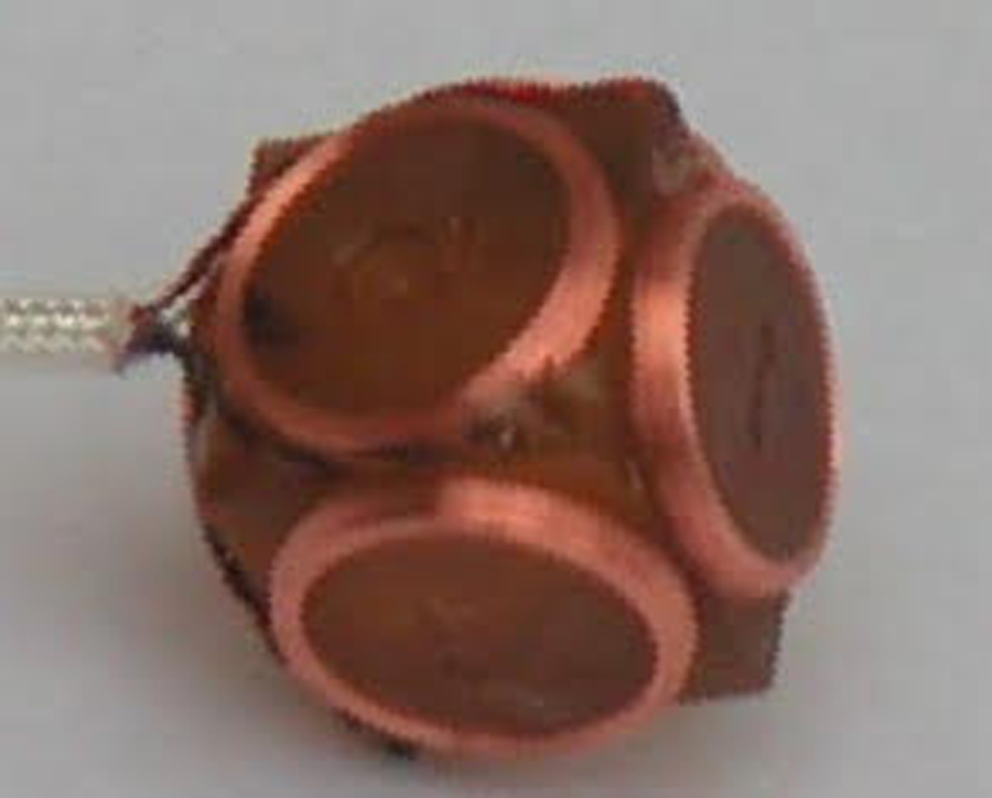
Sample cube sensor with a total of six coils, one at each side of the cube.

Alternatively, short wave trackers can be used that leverage the 1–5 MHz range (83), a frequency band where human tissues appear mostly transparent. Therefore, a sensor can be placed on the teeth of a subject, thus avoiding any problems associated with skin movement (83). The marker is a wireless RF reflector that scatters an applied RF field towards a detector array. In the most recent implementation three different frequencies (2.3, 3.1 and 4.2 MHz) were transmitted by a loop to the reflector, where each loop is only selectively sensitive to one of the frequencies. The reflected field can be measured by multiple MR compatible antennas, resulting in an overdetermined system for the marker position and orientation. The system currently requires calibration data and a neural network that matches position and orientation to the measured signals.

F.5. Probing the electrical properties of tissues

Different organs have different electrical properties, and these properties may change as a result of physiological motion. For example, the volume of blood in the heart varies by about twofold during the cardiac cycle; because blood and muscle have different tissue conductivities, about 0.66 and 0.39 S/m respectively, the overall conductivity of the heart changes as the blood/muscle ratio changes. Electric properties tend to vary with frequency: while tissue conductivity increases, tissue permittivity decreases with frequency (84). A cross section through a human model is shown in Figure 6a, which demonstrates spatial variations in conductivity.

Fig. 6:

a,b) Tissue conductivity at (a) low frequencies < 1 MHz, and (b) at 300 MHz (cross section through the IT’IS foundation Duke showing heart and lungs). c-e) The current density fields for two MRI coils placed over the human body are shown in (c,d) while (e) shows the tissue contribution to the mutual inductance between these two RF coils (Eq. 4). f) Reflection from tissue boundaries received back at the radar coil ‘R’ are displayed. Simulations were carried out in Sim4Life for a dipole antenna at 300 MHz, and were normalized to an input power of 1.0 W.

F.5.1. Impedance, inductance and coupling

Suppose for a moment that two electrodes were placed on the body, with a voltage V causing a current I to flow between them. One could easily calculate the resistance (inverse of conductivity):

$$R= \frac{V}{I}.$$ [3]

However, the current could have taken a multitude of different paths between the electrodes, and as such it is unclear which tissues contributed to what degree to the measured resistance. To take all possible paths into account, one must sum all contributions from all tissues on all paths using a volume integral. This integral relates $\sigma \left(\overrightarrow{x},t\right)$, the conductivity at all points $\overrightarrow{x}$ in the tissues at a given time t, the current field of the source and detector (${\overrightarrow{J}}_s\left(\overrightarrow{x},t\right)$ and ${\overrightarrow{J}}_d\left(\overrightarrow{x},t\right)$, respectively), and the measured impedance between the source and detector, $Z_{s,d}\left(t\right)$:

$$Z_{s,d}\left(t\right)=\iiint \frac{1}{\sigma \left(\overrightarrow{x},t\right)}{\overrightarrow{J}}_s\left(\overrightarrow{x},t\right)\cdot {\overrightarrow{J}}_d\left(\overrightarrow{x},t\right) dx dy dz.$$ [4]

The current fields are illustrated in Figure 6c,d and the inner part of the integral is illustrated in 6e. In general, the source and detector could be electrodes or RF antennas (85), and voltages as well as currents may be variable in time, e.g., in the RF range. In a way, the situation described in Eq. 4 is very complicated: as one monitors how the impedance $Z_{s,d}\left(t\right)$ varies in time, observed values depend on several multi-dimensional quantities. But on the other hand, as long as one is only concerned with detecting changes in conductivity, Eq. 4 shows that changes in $\sigma \left(\overrightarrow{x},t\right)$ at any location within the current field will likely be detected through changes in $Z_{s,d}\left(t\right)$. This impedance, $Z_{s,d}$, is typically referred to as the mutual inductance or coupling between RF coils.

F.5.2. Devices to measure changes in tissue properties

Devices that employ lower frequencies achieve greater tissue penetration, but low frequencies have more diffuse current fields resulting in more uniform energy losses through the body. In contrast, higher frequencies have lower penetration but better spatial localisation of changes in tissues electrical properties. In 1988, Buikman et al. used the MRI coil itself to measure changes in electrical properties (86), as the Q-factor of a birdcage RF coil was shown to change with both respiration and cardiac motion, reflecting changes in impedance in human tissues. A directional coupler was added to the RF chain to measure the reflected power, and for a constant forward power any change in impedance altered the absorbed and reflected power. Using the MRI coils as Buikman did (86), as opposed to additional hardware, can simplify workflows and synchronization between motion-related and MRI-related data acquisitions. One can employ multi transmit RF coils (87), or receive RF coils (88) for this purpose. Using arrays of RF coils may facilitate the separation of motions of different types, for example cardiac pulsation, respiratory motion and head motion (88–90).

The Pilot Tone uses MRI hardware for detection but separate hardware for the source. A constant low power single frequency reference signal outside of the imaging frequency band but within that of the MRI system is used. Using the MRI receiver coil for detection provides multiple detectors (coil elements) in close proximity to the organ of interest. The Pilot tone device has been used to monitor cardiac, respiratory and head motion, during free breathing cardiac cine (91) and 5D (respiratory and cardiac resolved) flow measurements (90), with results comparable to ECG. The Pilot Tone technology is available on some Siemens scanners under the denomination ‘BioMatrix’ and/or ‘Beat Sensor’ when used for respiration and cardiac gating, respectively.

More generally, when multiple sources and detectors are present, e.g., when using parallel transmit RF coils, the ‘scattering matrix’ formalism can be employed. Measuring a scattering matrix is done using directional couplers mounted on each of the transmit lines, to measure both the transmitted and reflected complex RF waveforms. In order to distinguish signal paths for each transmitter, time, space, or frequency multiplexing can be used (89). For example, cardiac triggers can be detected robustly (15 ms accuracy) within 20 ms of the ECG R-wave (92) and diaphragm position can be estimated robustly (1.4 mm accuracy) (87). Figure 7 shows what raw scattering data looks like, part c shows what the cardiac independent component trace looks like relative to the ECG signal and where automatic prospective triggers are detected. In another example, using EEG leads rather than MRI coil, data from an EEG cap was used to track head motion in 6DOF (93).

Fig. 7:

An example of a scattering matrix measurement showing (a) the real, (b) the imaginary components of the signal and (c) showing a linear combination of a and b that produces a cardiac trace that can be used for prospective cardiac gating as per ref (89).

F.5.3. Radar

Not unlike other types of waves, RF waves may be partly reflected when crossing boundaries between different materials. Especially at frequencies higher than those routinely involved in MRI, these reflections can be detected/mapped in an approach generally referred to as ‘radar’. The degree of reflection depends on the angle of incidence, the difference between the electromagnetic properties of the two tissues (94), and how large the wave is in relation to the surface (95). Figure 6f illustrates sources and magnitude of reflections at 300 MHz in the human body. Ultra-wide band radar measures reflections across a wide range of frequencies, often from DC up to 5 GHz (96). Given the change in dielectric properties across frequencies this enables deep penetration (using the low frequencies) along with identification of specific tissue interface signatures (from higher frequencies). Ultrawide band radar has been used in MRI (8,10), here the frequency range must be selected to prevent interference with the MR RF system. These have been developed for 300 MHz to 300 GHz using a low power pseudo random sequence (M-sequence) (94). This device has been demonstrated for monitoring respiration, cardiac (97) and head motion.

F.6 Qualitative waveforms, and quantitative calibration

Devices mentioned here typically provide waveforms that only indirectly relate to quantitative motion parameters. Qualitative cardiac waveforms can be generated from multiple observations using independent component analysis and then selecting the component near 1 Hz. The timing of cardiac-related events such as the atrial systole, the start/end of ventricular systole or the start of diastasis may be detected from these waveforms (92). Alternatively, breathing waveforms akin to that of respiratory bellows, of 1D diaphragm motion estimates (87) or of 2D heart motion estimates (98) can be extracted. Similar principles can be applied to detect head motion. To convert such qualitative waveforms into quantitative motion estimates, a patient-specific calibration scan, for example 30 s of MRI measurements of the diaphragm position, would be needed.

Overall, the main strength of RF based sensors may be their speed, as complete measurements take no longer than the duration of an excitation RF pulse, and in the case of radar and pilot-tone measurements can even be continuous.

G. Hybrid devices

For the most part, we do not see the various sensors and devices presented here as competing with each other: as long as each one brings its own type of information, that they do not interfere with each other and do not prove too cumbersome to use, they all may in principle find their role within future sensor suites. As these various devices gain in maturity and adoption, combinations are expected to become more common. For example, 3-axis hall effect magnetometers were combined with 3-axis pick-up coils (99) and with accelerometers (100) to obtain position and orientation estimates, see Fig. 8.

Fig. 8:

An example of a battery-powered hybrid device is shown here: While the 3D pickup coil senses the changing gradient fields through induction (Section F), the MEMS sensor incorporates a 3D accelerometer as well as a 3D angular rate sensor (Section C), and the Hall effect sensor (Section F) measures the magnitude and direction of the magnetic field, which is dominated by the static magnetic field. The resonant coil is used to detect the envelope of the RF pulses, for synchronization with the MRI acquisition. The microcontroller combines the various signals for motion estimation. A radiofrequency band near 2.4 GHz (far from the Larmor frequency) is used for wireless communication/operation.

Discussion and Conclusion

MRI signals are rich and versatile. In addition to soft tissue contrasts, they can capture temperature changes, field variations and physiological motion, for example. But MRI is not fast, and trying to do too much with its signals, all at the same time, detracts from its main purpose of capturing soft tissue contrasts. Ancillary devices often prove faster and better suited at measuring some of these parameters than MRI could ever be. For these reasons, traditional imaging modalities augmented by suites of sensors might represent the future of medical imaging in general, and of MRI in particular.

Sensors and ancillary devices are currently used in MRI primarily for timing purposes, i.e., to sync the acquisition/reconstruction process to physiological motion. Less frequently, they may be used to monitor variations in the scanner’s fields caused by eddy currents or susceptibility effects, for example. But to this day, sensor signals do not typically contribute directly to the MR images themselves: these images are reconstructed solely from k-space signals, as detected by the MRI equipment. We may, however, be on the cusp of important changes to this paradigm, as increasingly-present machine learning (ML) techniques are quite apt at combining different signal types in elaborate ways toward a coherent result. It is tempting to envision a future when signals from a variety of origins and hardware types may contribute much more directly, through ML-based algorithms, to the actual image contrasts and pixel values generated by MRI.

Currently, a main challenge to broader adoption remains the lack of availability for many of the sensors discussed here, which are often employed only in the labs where they were developed, and which were often adapted only to given scanners from given vendors. While this lack of broad availability and compatibility unavoidably slows down research developments, the ‘open-source hardware’ movement may, in time, offer solutions to this problem. The emergence of startup companies dedicated to the commercialization of some of these technologies, along with integration by major MRI vendors into some of their products, can also ensure broader availability and adoption.

As a limitation of the present work, new devices and variations on older ones continue to appear; we described here only the main types of devices that we were aware of, and we can only apologize for any we might have left out. Furthermore, only relatively small, adjunct devices were considered, as opposed to full-fledge imagers as in PET-MRI hybrid scanners for example.

In conclusion, sensors and ancillary devices have been staples of imaging suites ever since the early days of MRI. Since then, many new MRI-compatible devices have emerged that exploit a variety of physical principles to sense the imaged object and the imaging fields. Given the emergence of ML-based approaches for image reconstruction, and their aptitude at combining eclectic inputs into coherent outputs, the importance of sensors and ancillary devices is expected to grow.

References

- 1.Slipsager JM, Glimberg SL, Sogaard J, Paulsen RR, Johannesen HH, Martens PC, Seth A, Marner L, Henriksen OM, Olesen OV, Hojgaard L. Quantifying the Financial Savings of Motion Correction in Brain MRI: A Model-Based Estimate of the Costs Arising From Patient Head Motion and Potential Savings From Implementation of Motion Correction. J Magn Reson Imaging 2020;52(3):731–738. [DOI] [PubMed] [Google Scholar]
- 2.Littlejohns TJ, Holliday J, Gibson LM, Garratt S, Oesingmann N, Alfaro-Almagro F, Bell JD, Boultwood C, Collins R, Conroy MC, Crabtree N, Doherty N, Frangi AF, Harvey NC, Leeson P, Miller KL, Neubauer S, Petersen SE, Sellors J, Sheard S, Smith SM, Sudlow CLM, Matthews PM, Allen NE. The UK Biobank imaging enhancement of 100,000 participants: rationale, data collection, management and future directions. Nat Commun 2020;11(1):2624. [DOI] [PMC free article] [PubMed] [Google Scholar]
- 3.Andre JB, Bresnahan BW, Mossa-Basha M, Hoff MN, Smith CP, Anzai Y, Cohen WA. Toward Quantifying the Prevalence, Severity, and Cost Associated With Patient Motion During Clinical MR Examinations. J Am Coll Radiol 2015;12(7):689–695. [DOI] [PubMed] [Google Scholar]
- 4.Zaitsev M, Dold C, Sakas G, Hennig J, Speck O. Magnetic resonance imaging of freely moving objects: prospective real-time motion correction using an external optical motion tracking system. Neuroimage 2006;31(3):1038–1050. [DOI] [PubMed] [Google Scholar]
- 5.Odille F, Cindea N, Mandry D, Pasquier C, Vuissoz PA, Felblinger J. Generalized MRI reconstruction including elastic physiological motion and coil sensitivity encoding. Magn Reson Med 2008;59(6):1401–1411. [DOI] [PubMed] [Google Scholar]
- 6.Batchelor PG, Atkinson D, Irarrazaval P, Hill DL, Hajnal J, Larkman D. Matrix description of general motion correction applied to multishot images. Magn Reson Med 2005;54(5):1273–1280. [DOI] [PubMed] [Google Scholar]
- 7.Ehman RL, McNamara MT, Pallack M, Hricak H, Higgins CB. Magnetic resonance imaging with respiratory gating: techniques and advantages. AJR Am J Roentgenol 1984;143(6):1175–1182. [DOI] [PubMed] [Google Scholar]
- 8.Santelli C, Nezafat R, Goddu B, Manning WJ, Smink J, Kozerke S, Peters DC. Respiratory bellows revisited for motion compensation: preliminary experience for cardiovascular MR. Magn Reson Med 2011;65(4):1097–1102. [DOI] [PMC free article] [PubMed] [Google Scholar]
- 9.Lanzer P, Barta C, Botvinick EH, Wiesendanger HU, Modin G, Higgins CB. ECG-synchronized cardiac MR imaging: method and evaluation. Radiology 1985;155(3):681–686. [DOI] [PubMed] [Google Scholar]
- 10.Nacif MS, Zavodni A, Kawel N, Choi EY, Lima JA, Bluemke DA. Cardiac magnetic resonance imaging and its electrocardiographs (ECG): tips and tricks. Int J Cardiovasc Imaging 2012;28(6):1465–1475. [DOI] [PMC free article] [PubMed] [Google Scholar]
- 11.Konik A, Connolly CM, Johnson KL, Dasari P, Segars PW, Pretorius PH, Lindsay C, Dey J, King MA. Digital anthropomorphic phantoms of non-rigid human respiratory and voluntary body motion for investigating motion correction in emission imaging. Phys Med Biol 2014;59(14):3669–3682. [DOI] [PMC free article] [PubMed] [Google Scholar]
- 12.Rower LM, Radke KL, Hussmann J, Malik H, Uelwer T, Voit D, Frahm J, Wittsack HJ, Harmeling S, Pillekamp F, Klee D. Comparison of cardiac volumetry using real-time MRI during free-breathing with standard cine MRI during breath-hold in children. Pediatric radiology 2022. [DOI] [PMC free article] [PubMed] [Google Scholar]
- 13.Jarrahi B, Wanek J, Mehnert U, Kollias S. An fMRI-compatible multi-configurable handheld response system using an intensity-modulated fiber-optic sensor. Annu Int Conf IEEE Eng Med Biol Soc 2013;2013:6349–6352. [DOI] [PubMed] [Google Scholar]
- 14.Berglund J, van Niekerk A, Ryden H, Sprenger T, Avventi E, Norbeck O, Glimberg SL, Olesen OV, Skare S. Prospective motion correction for diffusion weighted EPI of the brain using an optical markerless tracker. Magn Reson Med 2021;85(3):1427–1440. [DOI] [PMC free article] [PubMed] [Google Scholar]
- 15.Herbst M, Maclaren J, Weigel M, Korvink J, Hennig J, Zaitsev M. Prospective motion correction with continuous gradient updates in diffusion weighted imaging. Magn Reson Med 2012;67(2):326–338. [DOI] [PubMed] [Google Scholar]
- 16.Aksoy M, Forman C, Straka M, Skare S, Holdsworth S, Hornegger J, Bammer R. Real-time optical motion correction for diffusion tensor imaging. Magn Reson Med 2011;66(2):366–378. [DOI] [PMC free article] [PubMed] [Google Scholar]
- 17.Thesen S, Heid O, Mueller E, Schad LR. Prospective acquisition correction for head motion with image-based tracking for real-time fMRI. Magn Reson Med 2000;44(3):457–465. [DOI] [PubMed] [Google Scholar]
- 18.Leemans A, Jones DK. The B-matrix must be rotated when correcting for subject motion in DTI data. Magn Reson Med 2009;61(6):1336–1349. [DOI] [PubMed] [Google Scholar]
- 19.Porter DA, Heidemann RM. High resolution diffusion-weighted imaging using readout-segmented echo-planar imaging, parallel imaging and a two-dimensional navigator-based reacquisition. Magn Reson Med 2009;62(2):468–475. [DOI] [PubMed] [Google Scholar]
- 20.Tisdall MD, Hess AT, Reuter M, Meintjes EM, Fischl B, van der Kouwe AJ. Volumetric navigators for prospective motion correction and selective reacquisition in neuroanatomical MRI. Magn Reson Med 2012;68(2):389–399. [DOI] [PMC free article] [PubMed] [Google Scholar]
- 21.Sachs TS, Meyer CH, Irarrazabal P, Hu BS, Nishimura DG, Macovski A. The diminishing variance algorithm for real-time reduction of motion artifacts in MRI. Magn Reson Med 1995;34(3):412–422. [DOI] [PubMed] [Google Scholar]
- 22.Maclaren J, Speck O, Stucht D, Schulze P, Hennig J, Zaitsev M. Navigator accuracy requirements for prospective motion correction. Magn Reson Med 2010;63(1):162–170. [DOI] [PMC free article] [PubMed] [Google Scholar]
- 23.Jochimsen TH, von Mengershausen M. ODIN-object-oriented development interface for NMR. J Magn Reson 2004;170(1):67–78. [DOI] [PubMed] [Google Scholar]
- 24.Layton KJ, Kroboth S, Jia F, Littin S, Yu H, Leupold J, Nielsen JF, Stocker T, Zaitsev M. Pulseq: A rapid and hardware-independent pulse sequence prototyping framework. Magn Reson Med 2017;77(4):1544–1552. [DOI] [PubMed] [Google Scholar]
- 25.Nielsen JF, Noll DC. TOPPE: A framework for rapid prototyping of MR pulse sequences. Magn Reson Med 2018;79(6):3128–3134. [DOI] [PMC free article] [PubMed] [Google Scholar]
- 26.Hoinkiss D, Cordes C, Konstandin S, Guenther M. Event-Based Traversing of Hierarchical Sequences Allows Real-Time Execution and Arbitrary Looping in a Scanner-Independent MRI Framework. Proceedings of the International Society for Magnetic Resonance in Medicine 2020; p. 1043. [Google Scholar]
- 27.Maclaren J, Lee KJ, Luengviriya C, Speck O, Zaitsev M. Combined prospective and retrospective motion correction to relax navigator requirements. Magn Reson Med 2011;65(6):1724–1732. [DOI] [PubMed] [Google Scholar]
- 28.Korin HW, Felmlee JP, Riederer SJ, Ehman RL. Spatial-frequency-tuned markers and adaptive correction for rotational motion. Magn Reson Med 1995;33(5):663–669. [DOI] [PubMed] [Google Scholar]
- 29.Maknojia S, Churchill NW, Schweizer TA, Graham SJ. Resting State fMRI: Going Through the Motions. Frontiers in neuroscience 2019;13:825. [DOI] [PMC free article] [PubMed] [Google Scholar]
- 30.Soares JM, Magalhaes R, Moreira PS, Sousa A, Ganz E, Sampaio A, Alves V, Marques P, Sousa N. A Hitchhiker’s Guide to Functional Magnetic Resonance Imaging. Frontiers in neuroscience 2016;10:515. [DOI] [PMC free article] [PubMed] [Google Scholar]
- 31.Isaieva K, Fauvel M, Weber N, Vuissoz PA, Felblinger J, Oster J, Odille F. A hardware and software system for MRI applications requiring external device data. Magn Reson Med 2022. [DOI] [PubMed] [Google Scholar]
- 32.Tokuda J, Fischer GS, Papademetris X, Yaniv Z, Ibanez L, Cheng P, Liu H, Blevins J, Arata J, Golby AJ, Kapur T, Pieper S, Burdette EC, Fichtinger G, Tempany CM, Hata N. OpenIGTLink: an open network protocol for image-guided therapy environment. Int J Med Robot 2009;5(4):423–434. [DOI] [PMC free article] [PubMed] [Google Scholar]
- 33.Maclaren J, Aksoy M, Ooi MB, Zahneisen B, Bammer R. Prospective motion correction using coil-mounted cameras: Cross-calibration considerations. Magn Reson Med 2018;79(4):1911–1921. [DOI] [PMC free article] [PubMed] [Google Scholar]
- 34.Aksoy M, Forman C, Straka M, Cukur T, Hornegger J, Bammer R. Hybrid prospective and retrospective head motion correction to mitigate cross-calibration errors. Magn Reson Med 2012;67(5):1237–1251. [DOI] [PMC free article] [PubMed] [Google Scholar]
- 35.Bammer R, Aksoy M, Liu C. Augmented generalized SENSE reconstruction to correct for rigid body motion. Magn Reson Med 2007;57(1):90–102. [DOI] [PMC free article] [PubMed] [Google Scholar]
- 36.Wallace TE, Afacan O, Kober T, Warfield SK. Rapid measurement and correction of spatiotemporal B0 field changes using FID navigators and a multi-channel reference image. Magn Reson Med 2020;83(2):575–589. [DOI] [PMC free article] [PubMed] [Google Scholar]
- 37.Beischer DE, Knepton JC, Jr Influence of Strong Magnetic Fields on the Electrocardiogram of Squirrel Monkeys (Saimiri Sciureus). Aerosp Med 1964;35:939–944. [PubMed] [Google Scholar]
- 38.Yazdi N, Ayazi F, Najafi K. Micromachined inertial sensors. In Proceedings of the IEEE, vol. 86, no. 8, pp. 1640–1659. 1998. p 17. [Google Scholar]
- 39.Myllyla TS, Elseoud AA, Sorvoja HS, Myllyla RA, Harja JM, Nikkinen J, Tervonen O, Kiviniemi V. Fibre optic sensor for non-invasive monitoring of blood pressure during MRI scanning. J Biophotonics 2011;4(1–2):98–107. [DOI] [PubMed] [Google Scholar]
- 40.van Niekerk A, van der Kouwe A, Meintjes E. A Method for Measuring Orientation Within a Magnetic Resonance Imaging Scanner Using Gravity and the Static Magnetic Field (VectOrient). IEEE Trans Med Imaging 2017;36(5):1129–1139. [DOI] [PMC free article] [PubMed] [Google Scholar]
- 41.Jafari Tadi M, Koivisto T, Pankaala M, Paasio A. Accelerometer-Based Method for Extracting Respiratory and Cardiac Gating Information for Dual Gating during Nuclear Medicine Imaging. Int J Biomed Imaging 2014;2014:690124. [DOI] [PMC free article] [PubMed] [Google Scholar]
- 42.Site of the ‘Hôpital Necker Enfants malades’ https://hopital-necker.aphp.fr/introducing-necker-enfants-malades-hospital. Last accessed on 6/6/2022.
- 43.Ludwig G The velocity of sound through tissues and the acoustic impedance of tissues. J Acoust Soc Am 1950;22:862–866. [Google Scholar]
- 44.Yengul SS, Barbone PE, Madore B. Dispersion in Tissue-Mimicking Gels Measured with Shear Wave Elastography and Torsional Vibration Rheometry. Ultrasound Med Biol 2019;45(2):586–604. [DOI] [PMC free article] [PubMed] [Google Scholar]
- 45.Muthupillai R, Lomas DJ, Rossman PJ, Greenleaf JF, Manduca A, Ehman RL. Magnetic resonance elastography by direct visualization of propagating acoustic strain waves. Science 1995;269(5232):1854–1857. [DOI] [PubMed] [Google Scholar]
- 46.Henneberg S, Hok B, Wiklund L, Sjodin G. Remote auscultatory patient monitoring during magnetic resonance imaging. J Clin Monit 1992;8(1):37–43. [DOI] [PubMed] [Google Scholar]
- 47.Frauenrath T, Hezel F, Renz W, d’Orth Tde G, Dieringer M, von Knobelsdorff-Brenkenhoff F, Prothmann M, Schulz Menger J, Niendorf T. Acoustic cardiac triggering: a practical solution for synchronization and gating of cardiovascular magnetic resonance at 7 Tesla. J Cardiovasc Magn Reson 2010;12:67. [DOI] [PMC free article] [PubMed] [Google Scholar]
- 48.Nassenstein K, Orzada S, Haering L, Czylwik A, Zenge M, Eberle H, Schlosser T, Bruder O, Muller E, Ladd ME, Maderwald S. Cardiac MRI: evaluation of phonocardiogram-gated cine imaging for the assessment of global und regional left ventricular function in clinical routine. Eur Radiol 2012;22(3):559–568. [DOI] [PubMed] [Google Scholar]
- 49.Günther M, Feinberg DA. Ultrasound-guided MRI: preliminary results using a motion phantom. Magn Reson Med 2004;52(1):27–32. [DOI] [PubMed] [Google Scholar]
- 50.Feinberg DA, Giese D, Bongers DA, Ramanna S, Zaitsev M, Markl M, Günther M. Hybrid ultrasound MRI for improved cardiac imaging and real-time respiration control. Magn Reson Med 2010;63(2):290–296. [DOI] [PMC free article] [PubMed] [Google Scholar]
- 51.Petrusca L, Cattin P, De Luca V, Preiswerk F, Celicanin Z, Auboiroux V, Viallon M, Arnold P, Santini F, Terraz S, Scheffler K, Becker CD, Salomir R. Hybrid ultrasound/magnetic resonance simultaneous acquisition and image fusion for motion monitoring in the upper abdomen. Investigative radiology 2013;48(5):333–340. [DOI] [PubMed] [Google Scholar]
- 52.Kording F, Yamamura J, Much C, Adam G, Schoennagel B, Wedegartner U, Ueberle F. Evaluation of an Mr Compatible Doppler-Ultrasound Device as a New Trigger Method in Cardiac Mri: A Quantitative Comparison to ECG. Biomed Tech (Berl) 2013;58 Suppl 1. [DOI] [PubMed] [Google Scholar]
- 53.Arvanitis CD, Livingstone MS, McDannold N. Combined ultrasound and MR imaging to guide focused ultrasound therapies in the brain. Phys Med Biol 2013;58(14):4749–4761. [DOI] [PMC free article] [PubMed] [Google Scholar]
- 54.Lee W, Chan H, Chan K, Fiorillo T, Fiveland E, Foo T, Mills D, Sabatini J, Shoudy D, Smith S, Bednarz B. A Magnetic Resonance Compatible E4D Ultrasound Probe for Motion Management of Radiation Therapy 2017; Washington DC. [DOI] [PMC free article] [PubMed] [Google Scholar]
- 55.Fraunhofer MEVIS. MR-compatible Ultrasound System and 3D Probe with real-time Tissue and Deformation Tracking. https://www.mevis.fraunhofer.de/en/solutionpages/mr-compatible-ultrasound-system-and-3d-probe-with-real-time-tissue-and-deformation-tracking.html.
- 56.Preiswerk F, Toews M, Cheng CC, Chiou JG, Mei CS, Schaefer LF, Hoge WS, Schwartz BM, Panych LP, Madore B. Hybrid MRI-Ultrasound acquisitions, and scannerless real-time imaging. Magn Reson Med 2017;78(3):897–908. [DOI] [PMC free article] [PubMed] [Google Scholar]
- 57.Schwartz BM, McDannold NJ. Ultrasound echoes as biometric navigators. Magn Reson Med 2013;69(4):1023–1033. [DOI] [PMC free article] [PubMed] [Google Scholar]
- 58.Madore B, Preiswerk F, Bredfeldt JS, Zong S, Cheng CC. Ultrasound-based sensors to monitor physiological motion. Med Phys 2021;48(7):3614–3622. [DOI] [PMC free article] [PubMed] [Google Scholar]
- 59.Madore B, Belsley G, Cheng CC, Preiswerk F, Kijewski MF, Wu PH, Martell LB, Pluim JPW, Di Carli M, Moore SC. Ultrasound-based sensors for respiratory motion assessment in multimodality PET imaging. Phys Med Biol 2022;67(2). [DOI] [PMC free article] [PubMed] [Google Scholar]
- 60.Willey D, Dickinson O, Overson D, Truong T-K, Robb F, Song A, Madore B, Darnell D. Wireless Physiological Motion Monitoring with an Integrated RF/Wireless Coil Array and MR-Compatible Ultrasound-Based System In: Proceedings of the International Society of Magnetic Resonance in Medicine 2022 London, UK. p. 3953. [Google Scholar]
- 61.Qin L, van Gelderen P, Derbyshire JA, Jin F, Lee J, de Zwart JA, Tao Y, Duyn JH. Prospective head-movement correction for high-resolution MRI using an in-bore optical tracking system. Magn Reson Med 2009;62(4):924–934. [DOI] [PMC free article] [PubMed] [Google Scholar]
- 62.Zahneisen B, Ernst T. Homogeneous coordinates in motion correction. Magn Reson Med 2016;75(1):274–279. [DOI] [PMC free article] [PubMed] [Google Scholar]
- 63.Hucker P, Dacko M, Zaitsev M. Combining prospective and retrospective motion correction based on a model for fast continuous motion. Magn Reson Med 2021;86(3):1284–1298. [DOI] [PubMed] [Google Scholar]
- 64.Olesen OV, Sullivan JM, Mulnix T, Paulsen RR, Hojgaard L, Roed B, Carson RE, Morris ED, Larsen R. List-mode PET motion correction using markerless head tracking: proof-of-concept with scans of human subject. IEEE Trans Med Imaging 2013;32(2):200–209. [DOI] [PubMed] [Google Scholar]
- 65.Frost R, Wighton P, Karahanoglu FI, Robertson RL, Grant PE, Fischl B, Tisdall MD, van der Kouwe A. Markerless high-frequency prospective motion correction for neuroanatomical MRI. Magn Reson Med 2019;82(1):126–144. [DOI] [PMC free article] [PubMed] [Google Scholar]
- 66.Maclaren J, Aksoy M, Bammer R. Contact-free physiological monitoring using a markerless optical system. Magn Reson Med 2015;74(2):571–577. [DOI] [PMC free article] [PubMed] [Google Scholar]
- 67.Spicher N, Kukuk M, Maderwald S, Ladd ME. Initial evaluation of prospective cardiac triggering using photoplethysmography signals recorded with a video camera compared to pulse oximetry and electrocardiography at 7T MRI. Biomed Eng Online 2016;15(1):126. [DOI] [PMC free article] [PubMed] [Google Scholar]
- 68.Antink CH, Lyra S, Paul M, Yu X, Leonhardt S. A Broader Look: Camera-Based Vital Sign Estimation across the Spectrum. Yearb Med Inform 2019;28(1):102–114. [DOI] [PMC free article] [PubMed] [Google Scholar]
- 69.VitalEye, Philips Medical Systems https://www.researchgate.net/figure/Visualization-of-the-built-in-the-bore-vital-sign-camera-VitalEye-Philips-Medical_fig1_349968858. Last accessed June 24th 2022.
- 70.Butler MJ, Crowe JA, Hayes-Gill BR, Rodmell PI. Motion limitations of non-contact photoplethysmography due to the optical and topological properties of skin. Physiological measurement 2016;37(5):N27–37. [DOI] [PubMed] [Google Scholar]
- 71.Schell JB, Kammerer JB, Hebrard L, Breton E, Gounot D, Cuvillon L, de Mathelin M. Towards a Hall effect magnetic tracking device for MRI. Annu Int Conf IEEE Eng Med Biol Soc 2013;2013:2964–2967. [DOI] [PubMed] [Google Scholar]
- 72.Dumoulin CL, Souza SP, Darrow RD. Real-time position monitoring of invasive devices using magnetic resonance. Magn Reson Med 1993;29(3):411–415. [DOI] [PubMed] [Google Scholar]
- 73.Derbyshire JA, Wright GA, Henkelman RM, Hinks RS. Dynamic scan-plane tracking using MR position monitoring. J Magn Reson Imaging 1998;8(4):924–932. [DOI] [PubMed] [Google Scholar]
- 74.Wang W, Dumoulin CL, Viswanathan AN, Tse ZTH, Mehrtash A, Loew W, Norton I, Tokuda J, Seethamraju RT, Kapur T, Damato AL, Cormack RA, Schmidt EJ. Real-time Active MR-tracking of Metallic Stylets in MR-guided Radiation Therapy. Magn Reson Med, in press 2015. [DOI] [PMC free article] [PubMed] [Google Scholar]
- 75.De Zanche N, Barmet C, Nordmeyer-Massner JA, Pruessmann KP. NMR probes for measuring magnetic fields and field dynamics in MR systems. Magn Reson Med 2008;60(1):176–186. [DOI] [PubMed] [Google Scholar]
- 76.Skope https://skope.swiss/.
- 77.Gilbert KM, Dubovan PI, Gati JS, Menon RS, Baron CA. Integration of an RF coil and commercial field camera for ultrahigh-field MRI. Magn Reson Med 2022;87(5):2551–2565. [DOI] [PubMed] [Google Scholar]
- 78.Haeberlin M, Kasper L, Barmet C, Brunner DO, Dietrich BE, Gross S, Wilm BJ, Kozerke S, Pruessmann KP. Real-time motion correction using gradient tones and head-mounted NMR field probes. Magn Reson Med 2015;74(3):647–660. [DOI] [PubMed] [Google Scholar]
- 79.Aranovitch A, Haeberlin M, Gross S, Dietrich BE, Wilm BJ, Brunner DO, Schmid T, Luechinger R, Pruessmann KP. Prospective motion correction with NMR markers using only native sequence elements. Magn Reson Med 2018;79(4):2046–2056. [DOI] [PubMed] [Google Scholar]
- 80.Nevo E; Method and apparatus to estimate location and orientation of objects during magnetic resonance imaging US 6,516,213. 2003.
- 81.Gholipour A, Polak M, van der Kouwe A, Nevo E, Warfield SK. Motion-robust MRI through real-time motion tracking and retrospective super-resolution volume reconstruction. Annu Int Conf IEEE Eng Med Biol Soc 2011;2011:5722–5725. [DOI] [PMC free article] [PubMed] [Google Scholar]
- 82.Afacan O, Wallace TE, Warfield SK. Retrospective correction of head motion using measurements from an electromagnetic tracker. Magn Reson Med 2020;83(2):427–437. [DOI] [PMC free article] [PubMed] [Google Scholar]
- 83.Schildknecht C, Brunner D, Schmid T, Pruessmann K. Advances in short-wave motion tracking: Jaw-mount markers and prospective motion correction. In: Proceedings of the International Society for Magnetic Resonance in Medicine, 2022. Londond, UK. [Google Scholar]
- 84.Gabriel S, Lau RW, Gabriel C. The dielectric properties of biological tissues: III. Parametric models for the dielectric spectrum of tissues. Phys Med Biol 1996;41(11):2271–2293. [DOI] [PubMed] [Google Scholar]
- 85.Malmivuo J Impedance Plethysmography. In: Malmivuo J, Plonsey R, editors. Bioelectromagnetism: principles and applications of bioelectric and biomagnetic fields USA: Oxford University Press; 1995. p 405–419. [Google Scholar]
- 86.Buikman D, Helzel T, Roschmann P. The rf coil as a sensitive motion detector for magnetic resonance imaging. Magn Reson Imaging 1988;6(3):281–289. [DOI] [PubMed] [Google Scholar]
- 87.Hess AT, Tunnicliffe EM, Rodgers CT, Robson MD. Diaphragm position can be accurately estimated from the scattering of a parallel transmit RF coil at 7 T. Magn Reson Med 2018;79(4):2164–2169. [DOI] [PMC free article] [PubMed] [Google Scholar]
- 88.Speier P, Fenchel M, Rehner R. PT-Nav: A Novel Respiratory Navigation Method for Continuous Acquisitions Based on Modulation of a Pilot Tone in the MR-Receiver. In: Proceedings of the European Society for Magnetic Resonance in Medicine and Biology Edinburgh, UK; 2015. p 128. [Google Scholar]
- 89.Jaeschke SHF, Robson MD, Hess AT. Scattering matrix imaging pulse design for real-time respiration and cardiac motion monitoring. Magn Reson Med 2019;82(6):2169–2177. [DOI] [PMC free article] [PubMed] [Google Scholar]
- 90.Falcao MBL, Di Sopra L, Ma L, Bacher M, Yerly J, Speier P, Rutz T, Prsa M, Markl M, Stuber M, Roy CW. Pilot tone navigation for respiratory and cardiac motion-resolved free-running 5D flow MRI. Magn Reson Med 2022;87(2):718–732. [DOI] [PMC free article] [PubMed] [Google Scholar]
- 91.Solomon E, Rigie DS, Vahle T, Paska J, Bollenbeck J, Sodickson DK, Boada FE, Block KT, Chandarana H. Free-breathing radial imaging using a pilot-tone radiofrequency transmitter for detection of respiratory motion. Magn Reson Med 2021;85(5):2672–2685. [DOI] [PMC free article] [PubMed] [Google Scholar]
- 92.Jaeschke SHF, Robson MD, Hess AT. Cardiac gating using scattering of an 8-channel parallel transmit coil at 7T. Magn Reson Med 2018;80(2):633–640. [DOI] [PMC free article] [PubMed] [Google Scholar]
- 93.Laustsen M, Andersen M, Xue R, Madsen KH, Hanson LG. Tracking of rigid head motion during MRI using an EEG system. Magn Reson Med 2022;88(2):986–1001. [DOI] [PMC free article] [PubMed] [Google Scholar]
- 94.Thiel F, Hein M, Schwarz U, Sachs J, Seifert F. Combining magnetic resonance imaging and ultrawideband radar: a new concept for multimodal biomedical imaging. Rev Sci Instrum 2009;80(1):014302. [DOI] [PubMed] [Google Scholar]
- 95.Wu T, Rappaport T, Collins C. The human body and millimeter-wave wireless communication systems: Interactions and implications In: 2015 IEEE International Conference on Communications (ICC), June 8–12, 2015. 2015. [Google Scholar]
- 96.Taoufik E, Nabila S, Ridha B. The ultra wide band radar system parameters in medical application. Journal of Electromagnetic Analysis and Applications 2011;5:147–154. [Google Scholar]
- 97.Thiel F, Kosch O, Seifert F. Ultra-wideband sensors for improved magnetic resonance imaging, cardiovascular monitoring and tumour diagnostics. Sensors (Basel) 2010;10(12):10778–10802. [DOI] [PMC free article] [PubMed] [Google Scholar]
- 98.Ludwig J, Speier P, Seifert F, Schaeffter T, Kolbitsch C. Pilot tone-based motion correction for prospective respiratory compensated cardiac cine MRI. Magn Reson Med 2021;85(5):2403–2416. [DOI] [PubMed] [Google Scholar]
- 99.van Niekerk A, van der Kouwe A, Meintjes E. Toward “plug and play” prospective motion correction for MRI by combining observations of the time varying gradient and static vector fields. Magn Reson Med 2019;82(3):1214–1228. [DOI] [PMC free article] [PubMed] [Google Scholar]
- 100.van Niekerk A, Meintjes E, van der Kouwe A. A Wireless Radio Frequency Triggered Acquisition Device (WRAD) for Self-Synchronised Measurements of the Rate of Change of the MRI Gradient Vector Field for Motion Tracking. IEEE Trans Med Imaging 2019;38(7):1610–1621. [DOI] [PMC free article] [PubMed] [Google Scholar]